Keypoint-Guided Optimal Transport

Abstract

Existing Optimal Transport (OT) methods mainly derive the optimal transport plan/matching under the criterion of transport cost/distance minimization, which may cause incorrect matching in some cases. In many applications, annotating a few matched keypoints across domains is reasonable or even effortless in annotation burden. It is valuable to investigate how to leverage the annotated keypoints to guide the correct matching in OT. In this paper, we propose a novel KeyPoint-Guided model by ReLation preservation (KPG-RL) that searches for the optimal matching (i.e., transport plan) guided by the keypoints in OT. To impose the keypoints in OT, first, we propose a mask-based constraint of the transport plan that preserves the matching of keypoint pairs. Second, we propose to preserve the relation of each data point to the keypoints to guide the matching. The proposed KPG-RL model can be solved by Sinkhorn’s algorithm and is applicable even when distributions are supported in different spaces. We further utilize the relation preservation constraint in the Kantorovich Problem and Gromov-Wasserstein model to impose the guidance of keypoints in them. Meanwhile, the proposed KPG-RL model is extended to the partial OT setting. Moreover, we deduce the dual formulation of the KPG-RL model, which is solved using deep learning techniques. Based on the learned transport plan from dual KPG-RL, we propose a novel manifold barycentric projection to transport source data to the target domain. As applications, we apply the proposed KPG-RL model to the heterogeneous domain adaptation and image-to-image translation. Experiments verified the effectiveness of the proposed approach.

Keywords: Keypoint-guided optimal transport, relation preservation, masked plan, manifold barycentric projection, heterogeneous domain adaptation, image-to-image translation

1 Introduction

Optimal Transport (OT) (Villani, 2009) is a mathematical tool for distribution alignment, mass transport, etc. OT has gained increasing attention in the machine learning community. OT aims to derive a transport map or plan between a source and a target distribution, such that the transport cost is minimized. Due to its capacity to exploit the geometric property of data, OT has been employed in many applications, e.g., computer vision (Bonneel et al., 2011; Solomon et al., 2015), natural language processing (Kusner et al., 2015; Huang et al., 2016; Alvarez-Melis and Jaakkola, 2018; Yurochkin et al., 2019), generative adversarial network (Arjovsky et al., 2017), domain adaptation (Courty et al., 2017), clustering (Ho et al., 2017; Huynh et al., 2021), anomaly detection (Tong et al., 2022), dataset comparison (Alvarez-Melis and Fusi, 2020), etc. OT has two typical formulations, i.e., Monge’s formulation (Monge, 1781) and Kantorovich’s formulation (Kantorovich, 1942). Kantorovich’s formulation (Kantorovich, 1942) relaxes Monge’s formulation and attracts broader studies in applications. We mainly deal with Kantorovich’s formulation in this paper. The original OT model, i.e., the Kantorovich Problem (Kantorovich, 1942) (KP), is a linear program that is computationally expensive. The entropy-regularized OT (Cuturi, 2013; Dessein et al., 2018) introduces the entropy as regularization to the OT model which is solved by the computationally cheaper Sinkhorn-Knopp algorithm (Sinkhorn and Knopp, 1967; Lin et al., 2022) allowing to use automatic differentiation (Genevay et al., 2018).

KP needs to transport all the mass of source distribution to exactly match the mass of target distribution. But in some cases, only partial mass of source and target distributions should be matched, e.g., the source or target samples contain outliers. To overcome this limitation, the partial OT (Guittet, 2002; Figalli, 2010; Caffarelli and McCann, 2010; Chapel et al., 2020), unbalanced OT (Chizat et al., 2018; Liero et al., 2018), and robust OT (Balaji et al., 2020; Mukherjee et al., 2021; Le et al., 2021) models are presented, that allow to transport only partial mass of distribution. Another extension of KP is the Gromov-Wasserstein (GW) model (Sturm, 2006; Mémoli, 2011) that computes the distance between metrics defined within each domain rather than between samples across domains as in KP.

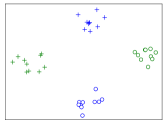
(a) Samples

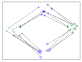
(b) KP

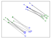
(c) GW

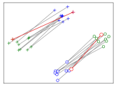
(d) KPG-RL (ours)

Figure 1: (a) Positive (cross) and negative (circle) samples of source (in blue) and target (in green) distributions. (b) KP distorts the data structure, leading to mismatch of some positive and negative samples. (c) GW model better preserves the data structure, but completely mismatches the samples. (d) Our proposed KPG-RL model utilizes some keypoints (red pairs) to guide the transport and produce correct matching.

In most of the above models, the main criterion for the optimal transport plan/matching is by the minimization of total transport distance or distortion over all samples. Though having achieved promising results in many applications, without any additional guidance, the OT models may lead to incorrect matching of samples. Figures 1(b) and  1(c) illustrate examples of incorrect matching produced by KP and GW models. In many applications, it is reasonable to annotate some paired keypoints across domains for guiding the matching in OT. For instance, in non-rigid point set or image registration (Myronenko and Song, 2010; Crum et al., 2004), a few keypoint pairs that should be matched are annotated in two point sets/images. In semi-supervised domain adaptation (Saito et al., 2019) and heterogeneous domain adaptation (Tsai et al., 2016), along with a large amount of labeled source domain data, there are a few labeled target domain data available, that could be directly taken as keypoints. Therefore, it is valuable and important to investigate how to take advantage of those keypoints to guide the correct matching in OT. Figure 1(d) shows an example that with the guidance of a few keypoints, the correctness of matching can be improved.

In this paper, we propose a novel KeyPoint-Guided model by ReLation preservation (KPG-RL) for leveraging the annotated keypoints to guide the matching in OT. In KPG-RL, we first preserve the matching of keypoint pairs in OT using a mask-based constraint of the transport plan. We then propose to preserve the relation of each data point to the keypoints in transport, enforcing the matching of the data points near to paired keypoints across domains. The proposed KPG-RL model is applicable even when distributions lie in different spaces, and can be solved by Sinkhorn’s algorithm. We further enforce the relation preservation constraint in KP and GW to impose the guidance of keypoints in them. To handle the applications where only partial mass should be transported, we extend the KPG-RL model to the partial OT setting, forming the partial-KPG-RL model.

Meanwhile, we present the dual formulation of KPG-RL model, enabling us to learn the transport plan and further the transport map using deep learning techniques. Specifically, we deduce the dual formulation of the $L_{2}$-regularized KPG-RL model, in which we parameterize the optimization variables, say potentials, with deep neural networks. The optimal transport plan can be calculated using the trained potentials, according to the strong duality. With given transport plan, we propose a novel Manifold Barycentric Projection (MBP) approach to transport source data to the target domain, dubbed KPG-RL-MBP. The KPG-RL-MBP transports the source samples to the barycenter of the conditional transport plan constrained into the target data manifold.

As applications, we apply the KPG-RL model to the heterogeneous domain adaptation (HDA) (Tsai et al., 2016) and image-to-image (I2I) translation (Isola et al., 2017). HDA is a transfer learning task that aims to transfer the knowledge of large-scale labeled source domain data to the target domain where a few labeled and larger amounts of unlabeled data are available for training. The “heterogeneity” implies that the source and target domain data are in heterogeneous feature spaces, e.g., generated by different deep networks. This heterogeneity poses a major obstacle in adapting the source-trained model to the target domain. We take the labeled target domain data and source class centers as keypoints and transport source domain data to the target domain by our KPG-RL model. Upon the transported source domain data and the labeled target domain data, a classification model is trained that is transferable to the target domain. Experiments show that the proposed KPG-RL model is effective for HDA.

We evaluate our KPG-RL-MBP in I2I translation task, in which we are given the images of two distinct domains with different styles, objects, etc. We consider the task that a large number of unpaired and a few paired images across the source and target domains are given in training. The goal is to transport the source images to the target domain using the paired images as guidance. We take the paired images as keypoints. We then apply the proposed KPG-RL-MBP to transport the source images to the target domain. Experiments on digits and natural animal images confirm that KPG-RL-MBP can realize the guidance of keypoints and produce clear transported images.

Our contributions are summarized as follows:

• We propose the novel KPG-RL model to leverage the given paired keypoints to guide the correct matching in OT. A mask-based constraint on the transport plan is applied to enforce the matching of keypoint pairs. We propose to preserve the relation of each data point to the keypoints to realize the guidance of keypoints.

• We apply the keypoint guidance in the existing OT models of KP and GW, of which the theoretical properties are presented. We extend the KPG-RL model to the partial OT setting where only partial mass is transported.

• We deduce the dual formulation of the KPG-RL model, based on which a novel manifold barycentric projection approach, KPG-RL-MBP, is proposed to transport the source data to the target domain.

• We apply the proposed method to HDA and I2I translation. Extensive experiments verify the effectiveness of the proposed approach.

This paper extends our conference version (Gu et al., 2022) with the following additional contributions. We present the dual formulation for the proposed KPG-RL model, which is an unconstrained optimization problem. To solve the dual problem, we parameterize the potentials using neural networks that are trained using mini-batch-based optimization algorithms. The transport plan is given by the strong duality using the learned potentials. With the learned transport plan, we propose a novel Manifold Barycentric Projection approach, KPG-RL-MBP, that transports source data to the barycenter of the conditional transport plan constrained into the target data manifold. We evaluate KPG-RL-MBP in semi-paired image-to-image translation, where a few paired and a large number of unpaired cross-domain images are available for training. We take the paired images are keypoints and utilize the proposed KPG-RL-MBP to transport source images to the target domain. Experiments on digit and natural animal images show that our approach can produce high-quality images and impose the guidance of keypoints.

In the following sections, we discuss the related works in Sect. 2, and introduce the background of OT in Sect. 3. In Sect. 4, we detail the proposed KPG-RL model. In Sect. 5, we elaborate on the dual KPG-RL model with the manifold barycentric projection. In Sect. 6, we apply our approach to HDA and I2I translation. Section 7 concludes this paper.

Notations.

$\Sigma_{m}=\{\bm{p}\in\mathbb{R}_{+}^{m}|\sum_{i}p_{i}=1\}$ is the probability simplex. $\langle\cdot,\cdot\rangle_{F}$ is the Frobenius dot product of two matrices. $\odot$ stands for the Hadamard product. $\mathbbm{1}_{m}$ denotes $m$-dimensional all-one vector. $\pi_{i,:}$ and $\pi_{:,j}$ are respectively the $i$-th row and $j$-th column of matrix $\pi$.

2 Related Works

We review below the most related OT models, HDA methods, and I2I translation approaches to our work.

OT models.

The GW model (Mémoli, 2011) seeks a “distance-preserving” transport plan such that the distance between transported points in the target domain is the same as the distance between the original points in source domain. Our KPG-RL model aims to use keypoint pairs to guide the matching (i.e., transport plan) in OT by preserving the relation of each point to the keypoints. Our “relation-preserving” scheme preserves the relation of data w.r.t. the given keypoints, different from the pairwise distance-preserving constraint in GW. We experimentally verified the effectiveness of relation-preserving scheme for introducing the guidance of keypoints in OT. From the computational point of view, GW is a non-convex quadratic program, while KPG-RL is a linear program. Lin et al. (2021) use the anchors to encourage clustering of data and to impose rank constraints on the transport plan to improve its robustness to outliers. The “anchors” in (Lin et al., 2021) are intermediate points in computation for improving robustness, different from the “keypoints” in this paper, which are the annotated paired data for guiding the matching in OT. Hierarchical OT (Yurochkin et al., 2019; Lee et al., 2019; Xu et al., 2020) transports points by dividing them into some subgroups and then derives the transport of these subgroups using OT. Different in goal and methodology from Hierarchical OT, we impose the guidance of keypoints for pursuing correct matching in OT by preserving the relation to the keypoints. We do not explicitly divide the points into subgroups, and there is no hierarchy in our method. TLB (Mémoli, 2011; Sato et al., 2020) is a lower bound of GW that can be computed faster. TLB takes the ordered distance of each point to all the points in the same domain as features, and then performs the Kantorovich formulation of OT using such features. Differently, our method uses a carefully designed relation of each point to the keypoints to impose the guidance of keypoints to the other points. Courty et al. (2017) constrain the cost function to encourage the matching of labeled data across source and target domains that share the same class labels for domain adaptation. They use the Laplacian regularization to preserve the data structure. Differently, we explicitly model the guidance of keypoints matching to the other data points in our OT formulation. The matching of paired keypoints is enforced by our mask-based constraint on the transport plan. Zhang et al. (2022) propose Masked OT model as a regularization term to preserve the local feature invariances between fine-tuned and pretrained graph neural network (GNN) for the fine-tuning of GNNs. Though the Masked OT (Zhang et al., 2022) shares similar spirits to the mask-based modeling in our method, our main contribution is the relation preservation for imposing the guidance of keypoints, different from (Zhang et al., 2022). For our mask-based modeling, it is utilized to impose the matching of keypoints with theoretical guarantee. While the mask in (Zhang et al., 2022) aims to preserve the local information of finetuned from pretrained models. The motivation and design of our mask are different from those in (Zhang et al., 2022).

HDA methods.

HDA methods could be roughly categorized into cross-domain mapping and common subspace learning methods. The cross-domain mapping approaches (Tsai et al., 2016; Yan et al., 2018; Shen and Guo, 2018; Mozafari and Jamzad, 2016; Zhou et al., 2019b) learn a transform to map the source features or model parameters to target domain to achieve adaptation. The common subspace learning approaches (Wang and Mahadevan, 2011; Wu et al., 2021; Yan et al., 2017; Zhou et al., 2019a; Wang and Breckon, 2022; Fang et al., In press, 2022) learn domain-specific projections to map source and target domain data into a common subspace such that their distributions are aligned. Our method for HDA belongs to the first category, and could be mostly related to (Yan et al., 2018). The method in (Yan et al., 2018) transports source samples to target domain using GW model regularized by the distance between the center of transported source samples and the center of labeled target samples having the same class labels. Different from (Yan et al., 2018), we take each labeled target data and its corresponding source class center as a keypoint pair and preserve the relation of each data point to the set of keypoints in each domain when conducting OT.

Image-to-image translation.

In the earlier supervised I2I translation works (Isola et al., 2017; Wang et al., 2018; Zhu et al., 2017b; Zhang et al., 2020; Bansal et al., 2018), researchers use many aligned cross-domain image pairs to obtain the translation model that translates the source images to the desired target images. However, training supervised translation is not very practical because of the difficulty and high cost of acquiring these large, paired training data in many tasks. Unsupervised I2I translation methods (Zhu et al., 2017a; Kim et al., 2017; Yi et al., 2017; Choi et al., 2021; Meng et al., 2021) use two large but unpaired sets of training images to convert images between representations. Though promising, the unsupervised methods require additional knowledge, e.g., domain-common knowledge (Choi et al., 2021), to guide the desired translation. Semi-supervised I2I translation approach (Mustafa and Mantiuk, 2020) leverages source images alongside a few source-target aligned image pairs for training, reducing the cost of human labeling or expert guidance in supervised I2I. In this paper, we tackle the semi-paired I2I translation task that many unpaired source and target images, and a few source-target aligned image pairs are available for training, because obtaining unlabeled target images could be reasonable in many applications. We take the given a few source-target aligned image pairs as keypoints and utilize our proposed KPG-RL-MBP method to translate the source images to the target domain.

3 Background on Optimal Transport

Kantorovich Problem (KP).

We consider two sets of data points, i.e., the source data $\bm{X}=\{{x}_{i}\}_{i=1}^{m}$ and the target data $\bm{Y}=\{{y}_{j}\}_{j=1}^{n}$, of which the empirical distributions are $\bm{p}=\sum_{i=1}^{m}p_{i}\delta_{x_{i}}$ and $\bm{q}=\sum_{j=1}^{n}q_{j}\delta_{y_{j}}$. With a slight abuse of notations, we may also denote $\bm{p}=(p_{1},p_{2},\cdots,p_{m})^{\top}\in\Sigma_{m}$ and $\bm{q}=(q_{1},q_{2},\cdots,q_{n})^{\top}\in\Sigma_{n}$ as the mass supported on $\bm{X}$ and $\bm{Y}$, respectively. We define the cost matrix between $\bm{X}$ and $\bm{Y}$ as $C=(C_{i,j})\in\mathbb{R}^{m\times n}$ with $C_{i,j}=c(x_{i},y_{j})$, where $c$ is a cost function, which is set to the squared $L_{2}$-distance of $x_{i}$ and $y_{j}$ in our experiments. OT aims to optimally transport $\bm{p}$ towards $\bm{q}$ at the smallest cost, formulated as the following Kantorovich Problem (KP):

$$\min_{\pi\in\Pi(\bm{p},\bm{q})}L_{kp}(\pi)\triangleq\langle\pi,C\rangle_{F},\mbox{ s.t. }\Pi(\bm{p},\bm{q})=\{\pi\in\mathbb{R}^{m\times n}_{+}|\pi\mathbbm{1}_{n}=\bm{p},\pi^{\top}\mathbbm{1}_{m}=\bm{q}\}.$$ (1)

When $c$ is taken as a distance metric (aka. ground metric), the minimum value of objective function in Eq. (1) is a distance between $\bm{p}$ and $\bm{q}$, named Wasserstein distance.

Partial OT model.

The KP in Eq. (1) takes the mass preserving assumption that all the mass of $\bm{p}$ is transported to exactly match the mass of $\bm{q}$. In many applications, only partial mass should be transported. The partial OT model (Figalli, 2010; Caffarelli and McCann, 2010) seeks the minimal cost of transporting only $s$ unit mass from $\bm{p}$ to $\bm{q}$, where $0\leqslant s\leqslant\min(\|\bm{p}\|_{1},\|\bm{q}\|_{1})$, formulated as

$$\min_{\pi\in\Pi^{s}(\bm{p},\bm{q})}L_{kp}(\pi),\mbox{ s.t. }\Pi^{s}(\bm{p},\bm{q})=\{\pi\in\mathbb{R}^{m\times n}_{+}|\pi\mathbbm{1}_{n}\leqslant\bm{p},\pi^{\top}\mathbbm{1}_{m}\leqslant\bm{q},\mathbbm{1}_{m}^{\top}\pi\mathbbm{1}_{n}=s\}.$$ (2)

Note that in partial OT, the total mass $\|\bm{p}\|_{1}$ and $\|\bm{q}\|_{1}$ are not necessarily equal.

Gromov-Wasserstein (GW) model.

If the data points $x_{i}$ and $y_{j}$ lie in different spaces, the distance between $x_{i}$ and $y_{j}$ may not be computed. The GW (Mémoli, 2011) model then minimizes the distortion when transporting the whole set of points from one space to another. The GW model relies on the intra-domain distance of source domain as $C^{s}=(C^{s}_{i,k})\in\mathbb{R}^{m\times m}$ and target domain as $C^{t}=(C^{t}_{j,l})\in\mathbb{R}^{n\times n}$, where $C^{s}_{i,k}$ is the distance between source domain data $x_{i}$ and $x_{k}$, and $C^{t}_{j,l}$ is the distance between target domain data $y_{j}$ and $y_{l}$. The GW model is given by

$$\min_{\pi\in\Pi(\bm{p},\bm{q})}L_{gw}(\pi)\triangleq\sum_{i,k=1}^{m}\sum_{j,l=1}^{n}\pi_{i,j}\pi_{k,l}|C^{s}_{i,k}-C^{t}_{j,l}|^{2}.$$ (3)

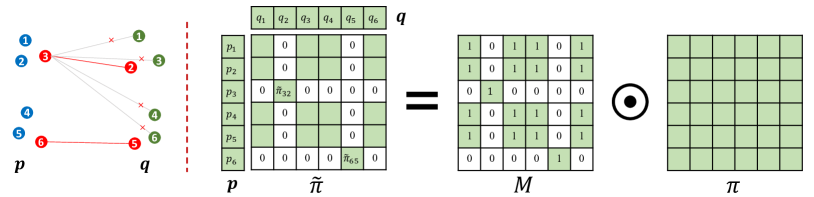
Figure 2: Example of modeling the matching of keypoints (red) using mask. The left part illustrates the matching of data points with keypoint pairs $\mathcal{K}=\{(3,2),(6,5)\}$. To preserve the matching of keypoint index pair $(i,j)$, e.g., $(3,2)$, the $i$-th row and $j$-th column of transport plan $\tilde{\pi}$ must be zeros except $\tilde{\pi}_{i,j}$. Therefore, we can model $\tilde{\pi}$ by $\tilde{\pi}=M\odot\pi$, where $M$ is the mask determined by the keypoints, and $\pi$ is to be optimized.

4 Keypoint-Guided Optimal Transport

This section details our proposed keypoint-guided model that leverages the keypoints to guide the matching in OT. The guidance is imposed by preserving the matching of keypoint pairs and the relation of each data point to the keypoints. We next discuss the preservation of matching of keypoints, introduce the modeling of relation, and present the keypoint-guided OT models. All the proofs of theorems or propositions are given in Appendix.

4.1 Preservation of Matching of Keypoints in Transport

We denote the set of keypoint index pairs as $\mathcal{K}=\{(i_{u},j_{u})\}_{u=1}^{U}$ with $U$ denoting the number of paired keypoints. We respectively denote $\mathcal{I}=\{i_{u}\}_{u=1}^{U}$ and $\mathcal{J}=\{j_{u}\}_{u=1}^{U}$ as the sets of source and target keypoint indexes. For the example illustrated in Fig. 2, $\mathcal{K}=\{(3,2),(6,5)\},\mathcal{I}=\{3,6\}$, and $\mathcal{J}=\{2,5\}$. To impose the guidance of these keypoints with indexes in $\mathcal{K}$ in deriving the transport plan in OT, we first guarantee the exact matching of the keypoint pairs. As illustrated in Fig. 2, we preserve the matching of keypoints in transport using a mask-based constraint of the transport plan, which is motivated by the following observation. If the paired keypoints $(i,j)\in\mathcal{K}$ are matched, the optimal transport plan $\tilde{\pi}$ satisfies that the $i$-th row and $j$-th column of $\tilde{\pi}$ must be zeros except $\tilde{\pi}_{i,j}$, which means that the all mass of source keypoint $x_{i}$ must be transported to target keypoint $y_{j}$ and $y_{j}$ can only receive the mass from $x_{i}$. For the example in Fig. 2, the 3-th row and 2-th column are zeros except that $\tilde{\pi}_{3,2}>0$. This sparsity of $\tilde{\pi}$ motivates us to model it as the Hadamard product of a mask matrix $M=(M_{i,j})\in\mathbb{R}^{m\times n}$ and a matrix $\pi\in\mathbb{R}_{+}^{m\times n}$ with positive entries, i.e.,

$$\tilde{\pi}=M\odot\pi,\mbox{ with }\tilde{\pi}_{i,j}=M_{i,j}\pi_{i,j}.$$ (4)

With Eq. (4), we define the admissible solution set for our keypoint-guided OT model as

$$\Pi(\bm{p},\bm{q};M)=\{\pi\in\mathbb{R}^{m\times n}_{+}|(M\odot\pi)\mathbbm{1}_{n}=\bm{p},(M\odot\pi)^{\top}\mathbbm{1}_{m}=\bm{q}\}.$$ (5)

Note that the $\pi$ in Eq. (5) is not necessarily a coupling. The entry $M_{i,j}$ of the mask matrix $M$ is set to 0 if $\tilde{\pi}_{i,j}$ needs to be 0, otherwise $M_{i,j}$ is set to 1. Figure 2 illustrates the mask-based modeling of Eq. (4). $M$ is constructed as in Proposition 1.

Proposition 1

Suppose that the mask matrix $M$ satisfies that

$$M_{i,j}=\begin{cases}1,&\mbox{ if }(i,j)\in\mathcal{K},\\ 0,&\mbox{ if }i\in\mathcal{I}$ and $(i,j)\notin\mathcal{K},\\ 0,&\mbox{ if }j\in\mathcal{J}$ and $(i,j)\notin\mathcal{K},\\ 1,&\mbox{ otherwise ({i}.{e}., $i\notin\mathcal{I}$ and $j\notin\mathcal{J}$)}.\end{cases}$$ (6)

and $p_{i}=q_{j}$, for $(i,j)\in\mathcal{K}$. Then, the transport plan $\tilde{\pi}=M\odot\pi$ with $\pi\in\Pi(\bm{p},\bm{q};M)$ preserves the matching of paired keypoints with index pairs in $\mathcal{K}$.

Proposition 1 indicates that if $p_{i}=q_{j}$, for $(i,j)\in\mathcal{K}$, the matching of keypoint pairs is preserved by the mask-based constraint. In this paper, for the convenience of description, we consider the case that $p_{i}=q_{j}$, $\forall(i,j)\in\mathcal{K}$. Note that this mask-based modeling in Eq. (4) is also applicable even for the case that there exist some $(i,j)\in\mathcal{K}$ such that $p_{i}\neq q_{j}$. For this case, we shall use different mask matrices. Please refer to the conference version (Gu et al., 2022) of this paper for the details.

4.2 Modeling the Relation to Keypoints

To use the keypoints to guide the matching in transport, we propose to preserve the relation of each point to the set of keypoints in transport. Figure 3 illustrates the relation within points of each distribution. For the data point $x_{k}\in\bm{X}$,

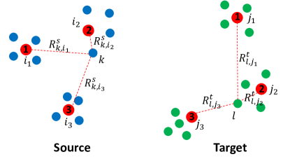
Figure 3: Illustration of relation of each point to the keypoints (red). In the keypoint-guided OT model, the relation should be preserved after transport.

its relation score to the keypoint $x_{i_{u}}$ for $i_{u}\in\mathcal{I}$ (illustrated by red circle in the left of Fig. 3) is defined as

$$R^{s}_{k,i_{u}}=\frac{e^{-C^{s}_{k,i_{u}}/\tau}}{\sum_{u^{\prime}=1}^{U}e^{-C^{s}_{k,i_{u}}/\tau}},\mbox{ }\forall i_{u}\in\mathcal{I},$$ (7)

$\tau$ is temperature set as $\tau=\rho*\max_{i,k}\{C^{s}_{i,k}\}$ in experiments. Similarly, for $y_{l}\in\bm{Y}$, its relation score to the keypoint $y_{j_{u}}$ for $j_{u}\in\mathcal{J}$ is defined as

$$R^{t}_{l,j_{u}}=\frac{e^{-C^{t}_{l,j_{u}}/\tau^{\prime}}}{\sum_{u^{\prime}=1}^{U}e^{-C^{t}_{l,j_{u}}/\tau^{\prime}}},\mbox{ }\forall j_{u}\in\mathcal{J},$$ (8)

$\tau^{\prime}$ is temperature set to $\rho*\max_{j,l}\{C^{t}_{j,l}\}$. The setting of $\tau$ and $\tau^{\prime}$ implies that the distances are divided by their maximum value, and normalized to $[0,1]$, which increases the robustness of the relation score to the scale of the distances. $\rho$ is a tunable parameter and set to 0.1 in our experiments, since 0.1 is a commonly used temperature in the softmax function (Chen et al., 2020; Khosla et al., 2020). We denote $R^{s}_{k}=(R^{s}_{k,i_{1}},R^{s}_{k,i_{2}},\cdots,R^{s}_{k,i_{U}})$ and $R^{t}_{l}=(R^{t}_{l,j_{1}},R^{t}_{l,j_{2}},\cdots,R^{t}_{l,j_{U}})$ that represent the relation of data points $x_{k}$ and $y_{l}$ to the keypoints in source and target domains, respectively. From the definition of the relation, the cross-domain points near to paired keypoints share similar relation to the keypoints in corresponding domain. For instance, in Fig. 3, $x_{k}$ and $y_{l}$ near to the paired keypoints with indexes $(i_{2},j_{2})$ have similar relation $R^{s}_{k}$ and $R^{t}_{l}$. Meanwhile, if $x_{k}$ is distant from all the keypoints, $R^{s}_{k}$ is close to a uniform probability vector.

4.3 Realizing Keypoint Guidance by Relation Preservation

Based on the relation given above, we define the guiding matrix

$$G=(G_{k,l})\in\mathbb{R}^{m\times n}\mbox{ by }G_{k,l}=d(R^{s}_{k},R^{t}_{l}),$$ (9)

where $d$ measures the dissimilarity of $R^{s}_{k}$ and $R^{t}_{l}$. Then, $G_{k,l}$ is small and even near to 0 if $R^{s}_{k}$ and $R^{t}_{l}$ are similar. $d$ is taken as the Jensen–Shannon divergence in this paper. We will study the effect of $d$ in experiments. By using the mask-based constraint of transport plan, the KeyPoint-Guided model by ReLation preservation (KPG-RL) is defined as

$$\min_{\pi\in\Pi(\bm{p},\bm{q};M)}L_{kpg}(\pi)\triangleq\langle M\odot\pi,G\rangle_{F}.$$ (10)

By the KPG-RL model in Eq. (10), first, the matching of keypoint pairs is enforced by the mask-based constraint of the transport plan. Second, the minimization of the objective function enforces that the optimal transport plan has larger entries in the locations where the entries of $G$ are smaller. Hence the cross-domain points corresponding to these locations (e.g., $k$ and $l$ shown in Fig. 3) that are near to paired keypoints tend to be matched. Based on the softmax-based formulations in Eqs. (7) and (8), $d(R_{k}^{s},R^{t}_{l})$ is mainly determined by the relation score to the closest keypoint(s), since relation scores to the distant keypoints are small or close to 0. This implies that the points are mainly guided by the closest keypoints in our KPG-RL model in Eq. (10). For the points distant from all the keypoints, their corresponding entries of $G$ are similar (close to zero) according to the definition of $G$. Therefore, the guidance of keypoints to these points is limited. To achieve correct matching of these points, additional information, e.g., point-wise cost or more keypoints, is needed.

Equation (10) is a linear program and can be solved by linear programming algorithms, e.g., the Simplex algorithm. Since Sinkhorn’s algorithm offers a lightspeed computation of the entropy-regularized OT (Cuturi, 2013), a natural question is that, can Sinkhorn’s algorithm be applied to the KPG-RL model with entropy regularization? We give the positive answer, and the details of the deduction are given in Appendix. The iterative formulas are

$$\bm{u}^{(l+1)}=\frac{\bm{p}}{K\bm{v}^{l}},\hskip 5.69046pt\bm{v}^{(l+1)}=\frac{\bm{q}}{K^{\top}\bm{u}^{(l+1)}},$$ (11)

where $K=M\odot e^{-G/\epsilon}$, $\epsilon$ is the coefficient of entropy regularization. The division operator used above is entry-wise. After iteration, the optimal transport plan is $\mbox{diag}(\bm{u})K\mbox{diag}(\bm{v})$.

Note that in this KPG-RL model in Eq. (10), the points in $\bm{X}$ and $\bm{Y}$ do not necessarily lie in the same space because we only need to compute the distance within each one of $\bm{X}$ and $\bm{Y}$. Therefore, the proposed KPG-RL model in Eq. (10) is applicable even when $\bm{p}$ and $\bm{q}$ are supported in different spaces. As mentioned in Sect. 1, the GW model is applicable for transport across different spaces. However, GW is a non-convex quadratic program and is often solved by the Frank-Walfe algorithm, in which a KP-like problem needs to be solved at each iteration by Sinkhorn’s algorithm or linear programming. Surprisingly, our KPG-RL model can be directly solved using Sinkhorn’s algorithm or linear programming without additional iteration, as discussed above.

4.4 Imposing Keypoint Guidance in KP/GW

We can impose the keypoint guidance in KP by adding $L_{kpg}(\pi)$ as a regularization term to KP, obtaining the following KPG-RL-KP model:

$$\min_{\pi\in\Pi(\bm{p},\bm{q};M)}\left\{\alpha L_{kp}(M\odot\pi)+(1-\alpha)L_{kpg}(\pi)=\langle M\odot\pi,\alpha C+(1-\alpha)G\rangle_{F}\right\},\alpha\in(0,1).$$ (12)

The KPG-RL-KP can be solved by Sinkhorn’s algorithm or linear programming, the same as the solution of KPG-RL model. Similarly, we define the KPG-RL-GW model in GW by

$$\min_{\pi\in\Pi(\bm{p},\bm{q};M)}\alpha L_{gw}(M\odot\pi)+(1-\alpha)L_{kpg}(\pi),\alpha\in(0,1).$$ (13)

The KPG-RL-GW model is solved using the Frank-Walfe algorithm. . The KPG-RL-KP/KPG-RL-GW models take both advantages of KP/GW and KPG-RL models, and could be helpful especially when the number of paired keypoints is small. We show in Sect. 4.6 that the KPG-RL-KP and KPG-RL-GW respectively provide a proper metric and a divergence under mild conditions. $\alpha$ is simply set to 0.5.

4.5 Extension to Partial OT

We now extend the above KPG-RL model to the more practical partial OT setting that only partial mass is transported. To do this, we first apply the above mask-based constraint of transport plan to the partial OT model in Eq. (2). We then add more constraints to enforce that all the mass of keypoints is transported to preserve the matching of keypoints. Finally, we define the partial-KPG-RL model as

$$\min_{\pi\in\Pi^{s}(\bm{p},\bm{q};M)}\left\{L_{kpg}(M\odot\pi)=\langle M\odot\pi,G\rangle_{F}\right\},$$ (14)

where $\Pi^{s}(\bm{p},\bm{q};M)=\{\pi\in\mathbb{R}^{m\times n}_{+}|(M\odot\pi)\mathbbm{1}_{n}\leqslant\bm{p},(M\odot\pi)^{\top}\mathbbm{1}_{m}\leqslant\bm{q},\mathbbm{1}_{m}^{\top}(M\odot\pi)\mathbbm{1}_{n}=s;(M\odot\pi)_{i,:}\mathbbm{1}_{n}=p_{i},\forall i\in\mathcal{I};\mathbbm{1}^{\top}_{m}(M\odot\pi)_{:,j}=q_{j},\forall j\in\mathcal{J}\}.$

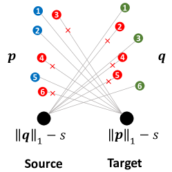
Figure 4: Illustration of dummy points (black circles) for source and target domains.

Chapel et al. (2020) propose a compelling method to solve the original partial OT problem in Eq. (2) by transforming the partial OT problem into an OT-like problem. Inspired by  Chapel et al. (2020), we add a dummy point with mass $\|\bm{q}\|_{1}-s$ for source domain (the left black circle in Fig. 4) and a dummy point with mass $\|\bm{p}\|_{1}-s$ for target domain (the right black circle in Fig. 4). We denote $\bar{\bm{p}}=(\bm{p}^{\top},\|\bm{q}\|_{1}-s)^{\top}$ and $\bar{\bm{q}}=(\bm{q}^{\top},\|\bm{p}\|_{1}-s)^{\top}$. As illustrated in Fig. 4, we aim to design the extended guiding matrix $\bar{G}$ and extended mask matrix $\bar{M}$ such that performing KPG-RL between $\bar{\bm{p}}$ and $\bar{\bm{q}}$ will transport $\|\bm{p}\|_{1}-s$ mass from source real data points to the target dummy point and transport $\|\bm{q}\|_{1}-s$ mass from source dummy point to target real data points. As a sequence, only $s$ mass of source and target real data points are matched. Meanwhile, the keypoints should not be matched to the dummy points because they are annotated data to guide the matching. To do this, we extend $G,M$ by

$$\bar{G}=\begin{bmatrix}G&\xi\mathbbm{1}_{n}\\ \xi\mathbbm{1}_{m}^{\top}&2\xi+A\end{bmatrix},\bar{M}=\begin{bmatrix}M&\bm{a}\\ \bm{b}^{\top}&1\end{bmatrix},$$

where $A>0$ and $\xi$ are two fixed scalars, and $\bm{a}\in\mathbb{R}^{m},\bm{b}\in\mathbb{R}^{n}$. The element $a_{i}$ of $\bm{a}$ is 0 if $i\in\mathcal{I}$, otherwise 1. The element $b_{j}$ of $\bm{b}$ is 0 if $j\in\mathcal{J}$, and 1 otherwise. By the following theorem, solving the optimal transport plan of problem (14) boils down to solving the problem $\mbox{min}_{\bar{\pi}\in\Pi(\bar{\bm{p}},\bar{\bm{q}};\bar{M})}\langle\bar{M}\odot\bar{\pi},\bar{G}\rangle_{F}$.

Theorem 2

Suppose $A>0$, $\sum_{i\in\mathcal{I}}p_{i}<s$, and $\sum_{j\in\mathcal{J}}q_{j}<s$, then the optimal transport plan $M\odot\pi^{*}$ of problem (14) is the $m$-by-$n$ block in the upper left corner of the optimal transport plan $\bar{M}\odot\bar{\pi}^{*}$ of problem $\mbox{min}_{\bar{\pi}\in\Pi(\bar{\bm{p}},\bar{\bm{q}};\bar{M})}\langle\bar{M}\odot\bar{\pi},\bar{G}\rangle_{F}$.

4.6 Theoretical Properties

In this section, we show that given prior “correct” paired keypoints, the KPG-RL-KP model provides a proper metric for distributions supported in the same space, and the the KPG-RL-GW model provides a divergence (in the sense of isomorphism) for distributions in distinct spaces, under mild conditions. Since the discrete distributions $\bm{p}=\frac{1}{m}\sum_{i}^{m}\delta_{x_{i}}$ (resp. $\bm{q}=\frac{1}{n}\sum_{j}^{n}\delta_{y_{j}}$) are invariant to the permutation of $\{x_{i}\}_{i=1}^{m}$ (resp. $\{y_{j}\}_{j=1}^{n}$), we assume that any two paired keypoints across domains share the same index. Therefore, the index set of paired keypoints is $\mathcal{K}=\{(i_{u},i_{u})\}_{u=1}^{U}$. We denote $\mathcal{P}_{\mathcal{I}}^{\mathcal{X}}$ as the set of discrete probability distributions supported on $m$ points in ground space $\mathcal{X}$ such that all distributions in $\mathcal{P}_{\mathcal{I}}^{\mathcal{X}}$ share the keypoint index set $\mathcal{I}=\{i_{u}\}_{u=1}^{U}$.

KPG-RL-KP providing a proper metric.

For distributions supported in the same space, the “correct” paired keypoints indicates that if $\bm{p}=\bm{q}$, each source keypoint is equal to its paired target keypoint, i.e., $x_{i_{u}}=y_{i_{u}}$, for any $i_{u}\in\mathcal{I}$. We denote

$$\mathcal{S}_{krk}(\bm{p},\bm{q})=\min_{\pi\in\Pi(\bm{p},\bm{q};M)}\sum_{i,j}{M_{i,j}\pi_{i,j}(\alpha C_{i,j}+(1-\alpha)G_{i,j})},$$ (15)

where $\alpha\in(0,1)$.

Theorem 3

Suppose $c$ is a proper distance in space $\mathcal{X}$ and $d$ is a proper distance in probability simplex $\Sigma_{U}$. Then, for any $\bm{p}$ and $\bm{q}$ in $\mathcal{P}_{\mathcal{I}}^{\mathcal{X}}$, given the “correct” paired keypoints stated above, $\mathcal{S}_{krk}(\bm{p},\bm{q})$ is a proper distance between $\bm{p}$ and $\bm{q}$.

KPG-RL-GW providing a divergence.

For any distribution $\bm{p}\in\mathcal{P}^{\mathcal{X}}_{\mathcal{I}}$ and $\bm{q}\in\mathcal{P}^{\mathcal{Y}}_{\mathcal{I}}$, $\bm{p}$ and $\bm{q}$ are said to be isomorphic if there exists a bijection $\sigma:[m]\longmapsto[m]$ such that $c(x_{i},x_{k})=c^{\prime}(y_{\sigma(i)},y_{\sigma(k)})$, and $p_{i}=q_{\sigma(i)}$, where $[m]=\{1,2,\cdots,m\}$, and $c$ and $c^{\prime}$ are respectively proper distances in spaces $\mathcal{X}$ and $\mathcal{Y}$. The keypoints are “correct” means that if $\bm{p}=\bm{q}$, $\sigma$ maps each source keypoint to its paired target keypoint, i.e., $\sigma(i_{u})=i_{u}$, for any $i_{u}\in\mathcal{I}$. We denote

$$\begin{split}\mathcal{S}_{krg}(\bm{p},\bm{q})=\min_{\pi\in\Pi(\bm{p},\bm{q};M)}\sum_{i,j}&\Big{[}\alpha\Big{(}\sum_{k,l}(M\odot\pi)_{i,j}(M\odot\pi)_{k,l}|C^{s}_{i,k}-C^{t}_{j,l}|^{2}\Big{)}\\ &+(1-\alpha)(M\odot\pi)_{i,j}G_{i,j}\Big{]},\end{split}$$ (16)

where $\alpha\in(0,1)$.

Theorem 4

Suppose $c$ and $c^{\prime}$ are proper distances in spaces $\mathcal{X}$ and $\mathcal{Y}$. Suppose $d$ is a divergence in probability simplex $\Sigma_{U}$. Then, for any $\bm{p}$ in $\mathcal{P}_{\mathcal{I}}^{\mathcal{X}}$ and any $\bm{q}$ in $\mathcal{P}_{\mathcal{I}}^{\mathcal{Y}}$, given the “correct” paired keypoints stated above, $\mathcal{S}_{krg}(\bm{p},\bm{q})=0$ if and only if $\bm{p}$ and $\bm{q}$ are isomorphic.

5 Learning Transport Map for Keypoint-Guided Optimal Transport

In Sect. 4, we have discussed the keypoint-guided optimal transport model in primal formulation (i.e., Eq. (10)) that is solved by linear programming or Sinkhorn iteration. In this section, we will develop a deep-learning-based approach for estimating the transport plan and map based on the dual formulation of KPG-RL. Our approach is inspired by (Seguy et al., 2018) that studies the KP. Seguy et al. (2018) start with the dual problem of the entropy or $L_{2}$-regularized KP model, which is solved by the training of deep learning. Based on the learned transport plan, they propose the Barycentric Projection (BP) to transport source data to the target domain. Inspired by Seguy et al. (2018), we will first develop the dual formulation of the $L_{2}$-regularized KPG-RL model and solve it by training deep neural networks. Based on the learned transport plan, we further propose a novel Manifold Barycentric Projection (MBP) to transport source samples to the target domain, for tackling the issue of the blur of transported samples by BP.

Dual formulation of $L_{2}$-regularized KPG-RL.

There are mainly two types of regularization, i.e., entropy regularization (Cuturi, 2013) and $L_{2}$-regularization (Seguy et al., 2018; Blondel et al., 2018) in OT model. We adopt the $L_{2}$-regularization for our purpose because we find that the $L_{2}$-regularization makes the training more stable than the entropy regularization for the smaller regularization coefficient in experiments. The dual formulation of the entropy-regularized KPG-RL can be deduced analogously, left as our future work. The $L_{2}$-regularized KPG-RL model is given by

$$\min_{\pi\in\Pi(\bm{p},\bm{q};M)}\langle M\odot\pi,G\rangle_{F}+\epsilon\chi^{2}(M\odot\pi\|\bm{p}\times\bm{q}),$$ (17)

where $\chi^{2}(M\odot\pi\|\bm{p}\times\bm{q})=\sum_{i=1}^{m}\sum_{j=1}^{n}\left(\frac{M_{i,j}\pi_{i,j}}{p_{i}q_{j}}\right)^{2}p_{i}q_{j}$. The following theorem 5 provides the dual formation of problem (17).

Theorem 5

The $L_{2}$-regularized KPG-RL model in Eq. (17) takes the dual formmulation

$$\max_{\phi,\psi}\sum_{i=1}^{m}\phi(x_{i})p_{i}+\sum_{j=1}^{n}\psi(y_{j})q_{j}-\frac{1}{4\epsilon}\sum_{i,j}M_{i,j}(\phi(x_{i})+\psi(y_{j})-G_{i,j})_{+}^{2}p_{i}q_{j},$$ (18)

where $a_{+}=\max\{a,0\}$. Let $\phi^{*}$, $\psi^{*}$ be the optimal solution of Eq. (18), then the optimal transport plan $M\odot\pi^{*}$ of Eq. (17) satisfies

$$(M\odot\pi^{*})_{i,j}=\frac{1}{2\epsilon}M_{i,j}(\phi^{*}(x_{i})+\psi^{*}(y_{j})-G_{i,j})_{+}p_{i}q_{j}.$$ (19)

Equation (18) is an unconstrained optimization problem w.r.t. continuous functions $\phi,\psi$. We use neural networks $\phi_{\theta},\psi_{\theta}$ to parameterize $\phi,\psi$ respectively and use mini-batch stochastic gradient descent to optimize $\theta$. Specifically, in each iteration, we sample mini-batch samples from $\bm{p},\bm{q}$, calculate the objective function in Eq. (18) on the mini-batch samples, compute gradient w.r.t. $\theta$ using backpropagation, and update $\theta$ by gradient descent. Such a mini-batch-based optimization process enables the keypoint-guided optimal transport model to scale to the distributions supported on a larger number ($m$ and $n$) of samples, because we only need a mini-batch of samples to calculate the objective function in each iteration. Once the optimization process is completed, we can recover the optimal transport plan by Eq. (19).

Manifold barycentric projection.

With the optimal transport plan, we next discuss how to transport the source data to the target domain. As mentioned before, Seguy et al. (2018) propose the BP to transport the source data to the target domain, which can be directly applied to our approach using our learned transport plan. Then, the BP ($T_{BP}$) is given by

$$T_{BP}=\arg\min_{T^{\prime}}\sum_{i=1}^{m}\sum_{j=1}^{n}(M\odot\pi^{*})_{i,j}\|y_{j}-T^{\prime}(x_{i})\|^{2}_{2}.$$ (20)

However, for source sample $x$, the transported sample $T_{BP}(x)$ by BP is blurry as shown in Fig. 11(c). This is mainly because that $T_{BP}(x)$ is close to the weighted average of target samples $\{y_{j}\}_{j=1}^{n}$, according to Eq. (20).

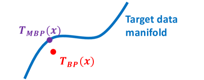
Figure 5: Illustration of our manifold barycentric projection for transporting source data to the target domain. The image $T_{BP}(x)$ of barycentric projection is outside the target data manifold and is blurry. The transported data $T_{MBP}(x)$ by our proposed manifold barycentric projection is constrained to the target data manifold.

We analyze that the blur caused by the BP is probably because the projected data $T_{BP}(x)$ may not be in the target data manifold. To make the transported data clear, we propose the Manifold Barycentric Projection (MBP) that enforces the transported data to near to $T_{BP}(x)$ constrained into the target data manifold. Figure 5 illustrates our idea. The transport map is learned from the following model:

$$T_{MBP}=\arg\min_{T^{\prime}}\lambda\sum_{i=1}^{m}\sum_{j=1}^{n}(M\odot\pi^{*})_{i,j}\|y_{j}-T^{\prime}(x_{i})\|^{2}_{2}+\mathcal{L}_{M}(T^{\prime}),$$ (21)

where the first term enforces the transported data is near to that of the barycentric projection, the second term encourages the transported data to lie in the target data manifold, and $\lambda$ is a hyper-parameter for balancing the importance of the two terms and is set to 10 in experiments. For simplicity, we use the loss of WGAN-GP (Gulrajani et al., 2017) as $\mathcal{L}_{M}$, because WGAN-GP is often used for modeling the manifold of data (Pandey et al., 2021). $\mathcal{L}_{M}$ is given by

$$\mathcal{L}_{M}(T^{\prime})=\max_{D}{\sum_{i=1}^{m}D(T^{\prime}(x_{i}))p_{i}-\sum_{j=1}^{n}D(y_{j})q_{j}+\beta\mathbb{E}_{\hat{x}\sim\hat{\bm{p}}}(\|\nabla_{\hat{x}}D(\hat{x})\|_{2}-1)^{2}},$$ (22)

where $\hat{\bm{p}}$ denotes the samples uniformly along lines between pairs of points sampled from the transported source distribution $T^{\prime}_{\#}\bm{p}$ and target distribution $\bm{q}$, and $D$, named discriminator, is a neural network that outputs a scalar. Following Gulrajani et al. (2017), $\beta$ is set to 10, and the gradient of $\hat{x}$ w.r.t. $T^{\prime}$ is stopped. Equation (21) is optimized by the mini-batch stochastic gradient descent/ascent to update $T^{\prime}$/$D$, respectively. With the learned $T_{MBP}$, given the source domain test sample $x$ even outside the training set, we transport it to the target domain by $T_{MBP}(x)$.

6 Experiments

We evaluate our method on toy data, HDA, and I2I translation experiments. Source codes will be available at https://github.com/XJTU-XGU/KPG-RL.

6.1 Toy Experiments

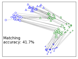
(a) KP

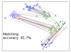
(b) KPG-RL-KP (w/ 2 keypoints)

(c) KPG-RL-KP (w/ 3 keypoints)

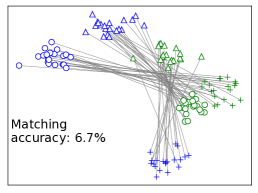
(d) GW

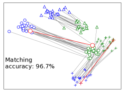
(e) KPG-RL-GW (w/ 2 keypoints)

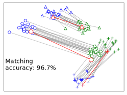
(f) KPG-RL-GW (w/ 3 keypoints)

Figure 6: Matching produced by (a) KP, (b) KPG-RL-KP model given 2 keypoint pairs, (c) KPG-RL-KP model given 3 keypoint pairs, (d) GW model, (e) KPG-RL-GW model given 2 keypoint pairs, and (f) KPG-RL-GW model given 3 keypoint pairs.

Toy experiments for evaluating KPG-RL-KP and KPG-RL-GW.

As illustrated in Fig. 6, in this toy data experiment, each of the source (blue) and target (green) distributions is a Gaussian mixture composed of three distinct Gaussian components indicated by different shapes where the same shapes indicate points of the same class. In Fig. 6, we have the following observations. In Fig. 6(a), in the KP model, the points in each component of target distribution are mismatched to points in different classes of source distributions, and only a small fraction of target points are correctly matched to source points belonging to the same class. In Fig. 6(b), given 2 keypoint pairs (from distinct classes), the KPG-RL-KP model apparently improves the correctness of matching. In Fig. 6(c), the KPG-RL-KP model mainly matches the source points to the target points belonging to the same class, thanks to the given 3 keypoint pairs. This implies that our proposed keypoint-guided model does help to produce correct matching in OT by leveraging the given a few keypoint pairs. In Figs. 6(d), 6(e) and 6(f), the proposed KPG-RL-GW model improves the correctness of matching of GW model by leveraging the guidance of given keypoints pairs.

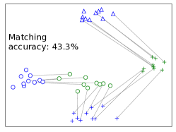
(a) Partial-OT

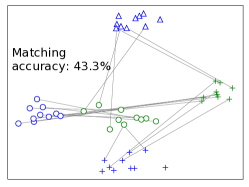
(b) Partial-GW

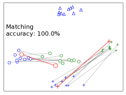
(c) Partial-KPG-RL (ours)

Figure 7: Matching produced by (a) partial-OT model, (b) partial-GW model, and (c) our proposed partial-KPG-RL model.

Toy experiments for evaluating Partial-KPG-RL.

Figure 7 illustrates the toy data experiment for evaluating the partial-KPG-RL model. In Fig. 7, the source (blue) and target (green) distributions are Gaussian mixtures. The source (resp. target) distribution is composed of three (resp. two) distinct Gaussian components indicated by different shapes where the same shapes indicate the points of the same class. When conducting OT, the source class data represented by “$\bigtriangleup$” should not be transported. In Figs. 7(a) and 7(b), we can observe that both the partial-OT model (defined in Eq. (2)) and the partial-GW model (Chapel et al., 2020) wrongly transport some source points of class “$\bigtriangleup$” to target domain and lead to lower matching accuracy. With the guidance of a few keypoints (red pairs), our proposed partial-KPG-RL model does not transport the source points of class “$\bigtriangleup$” to target domain and apparently improves the matching accuracy, as in Fig. 7(c).

6.2 Heterogeneous Domain Adaptation

6.2.1 Closed-Set Heterogeneous Domain Adaptation

In closed-set HDA (in what follows, we refer to the closed-set HDA by HDA), we are given labeled source data $\{(x_{i},t_{i})\}_{i=1}^{m}$, a few labeled target data $\{y_{j},\bar{t}_{j}\}_{j=1}^{n_{l}}$, and unlabeled target domain data $\{y_{j}\}_{j=n_{l}+1}^{n}$, where $m\gg n_{l}$, $n\gg n_{l}$, $x_{i}$ and $y_{j}$ are features, and $t_{i}$ and $\bar{t}_{j}$ are respectively the class labels of $x_{i}$ and $y_{j}$. The source and target data share the same label space (the set of classes). The heterogeneity means that $x_{i}$ and $y_{j}$ are from different spaces/modalities. The goal of HDA is to train a classification model using the given data to predict the label of unlabeled target domain data, leveraging the knowledge of labeled source domain data. The main challenge is that the domain gap between heterogeneous source and target distributions supported in distinct spaces hinders the direct employment of the source-trained model in the target domain.

We tackle the problem of HDA using our proposed KPG-RL model as follows. We first transport the source domain data using our KPG-RL model to the target domain. More concretely, in KPG-RL, each labeled target domain data and the source domain class center of the same class are taken as a matched keypoint pair. The KPG-RL model is then performed between empirical distributions of the source domain data along with class centers and the target domain data (including labeled and unlabeled data). Based on the produced optimal transport plan, we transport the source domain data using the barycentric mapping (Reich, 2013) to the target domain. The barycentric mapping $B_{\pi}$ associated to transport plan $\pi$ is defined by $B_{\pi}(x_{i_{0}})=\frac{1}{\sum_{j=1}^{n}\pi_{i_{0},j}}\sum_{j=1}^{n}\pi_{i_{0},j}y_{j}.$ Note that our MBP (presented in Sect. 5) learns transport map by training deep networks, which may be suitable for the applications where we need to transport source samples outside the training set, e.g., I2I translation discussed in Sect. 6.3. For simplicity, we directly adopt the barycentric mapping for the HDA experiments. Finally, we train the classification model (taken as a kernel SVM) on the transported source domain data (using their class label before transport) and the labeled target domain data, which is applied to the target domain test data. In the kernel SVM, we use the Gaussian $k(x,y)=\exp(-\gamma\|x-y\|_{2}^{2})$, where $\gamma$ is set to the reciprocal of the dimension of $x$. $\epsilon$ is set to 0.005.

Table 1: Accuracy on Office-31 for HDA. “A”, “W”, and “D” are respectively the domains of amazon, webcam, and dslr. “$\cdot\rightarrow*$” denotes a heterogeneous adaptation task where $\cdot$ and $*$ are respectively source domain using DeCAF₆ feature and target domain using ResNet-50 feature.

Method	A$\rightarrow$A	A$\rightarrow$D	A$\rightarrow$W	D$\rightarrow$A	D$\rightarrow$D	D$\rightarrow$W	W$\rightarrow$A	W$\rightarrow$D	W$\rightarrow$W	Avg
Labeled-target-only	45.3	69.2	67.3	45.3	69.2	67.3	45.3	69.2	67.3	60.6
STN	58.7	84.8	80.0	51.2	91.0	83.8	52.8	95.2	87.4	76.1
SSAN	56.8	89.7	87.1	54.2	82.6	90.3	50.0	85.8	85.8	75.8
DDACL	44.2	63.2	64.2	43.9	77.4	70.6	39.8	64.5	73.2	60.1
CDSPP	55.5	79.7	76.5	43.2	80.6	84.2	47.4	78.7	84.5	70.0
SGW	49.7	77.7	73.6	49.4	78.4	73.6	48.7	80.3	74.5	67.3
GW	33.6	41.6	35.5	39.7	40.0	31.7	34.8	34.5	29.0	35.6
GW (w/ mask)	41.3	71.6	69.7	41.9	71.2	69.8	40.3	71.6	69.7	60.8
HOT	39.0	44.8	40.0	31.3	52.6	44.8	29.7	60.0	56.5	44.3
HOT (w/ mask)	45.2	60.3	57.4	48.9	63.5	59.2	40.3	67.1	61.4	55.9
TLB	29.4	36.5	43.2	24.5	31.3	51.0	23.6	31.9	49.7	35.7
TLB (w/ mask)	42.5	66.3	64.7	38.5	68.5	65.9	43.1	68.2	67.3	58.3
KPG (w/ dist)	55.2	60.7	71.6	51.3	71.9	77.1	48.7	70.0	77.7	64.9
KPG-RL-GW	58.7	92.9	84.2	57.4	95.5	87.1	55.5	95.5	90.0	79.6
KPG-RL (LP)	56.5	93.6	83.2	58.1	94.5	86.8	55.8	95.2	89.7	79.3
KPG-RL (SH)	60.0	91.6	83.6	57.4	95.8	87.7	59.1	95.2	88.4	79.9

We compare our method with the following baseline methods, including 1) “Labeled-target-only” that trains the kernel SVM using the labeled target data; 2) the OT methods of “GW”, “HOT”, and “TLB” that transport source domain data using barycentric mapping induced by the transport plan of GW (Mémoli, 2011), Hierarchical OT (Lee et al., 2019), and TLB (Mémoli, 2011), and then train the kernel SVM on the transported data and labeled target domain data; 3) the typical HDA methods of “SGW” (Yan et al., 2018) and “STN” (Yao et al., 2019), and the recent HDA methods of “SSAN” (Li et al., 2020), “DDACL” (Yao et al., 2020) and “CDSPP” (Wang and Breckon, 2022). We conduct experiments on Office-31 (Saenko et al., 2010) dataset. On Office-31, we use the DeCAF₆ (Donahue et al., 2014) features and the features extracted by ResNet-50 (He et al., 2016) pretrained on ImageNet (Russakovsky et al., 2015) to respectively build source and target domains for constructing heterogeneous adaptation tasks. In each task, one labeled data (1-shot) for each class is given in the target domain. Note that all the methods use the same training data (including labeled source and target domain data, and unlabeled target domain data) and test data.

Table 1 reports the results on Offce-31 dataset. In Table 1, “KPG-RL (SH)” and “KPG-RL (LP)” denote our entropy-regularized KPG-RL model solved using Sinkhorn’s algorithm and our KPG-RL model solved by linear programming, respectively. KPG-RL (SH) achieves marginally better average accuracy than KPG-RL (LP), which could be because the barycentric mapping based on the more dense transport plan optimized by Sinkhorn’s algorithm is more robust to incorrect matching. We also observe that KPG-RL-GW achieves slightly lower average accuracy than KPG-RL (SH), and KPG-RL (SH) is more computationally efficient as discussed in Sect. 4. “KPG (w/ dist)” is the approach that imposes the guidance of keypoints using distance preservation in our framework, i.e., $R^{s}_{k,i_{u}}$ and $R^{t}_{l,j_{u}}$ in Eqs. (7) and (8) are taken as $C^{s}_{k,i_{u}}$ and $C^{t}_{l,j_{u}}$, respectively. KPG-RL (SH) improves the accuracy of KPG (w/ dist) by 15%, implying that our relation-preserving scheme is more effective for imposing the guidance of keypoints than the distance-preserving scheme. Table 1 shows that the results of GW, HOT, and TLB are inferior to that of Labeled-target-only, indicating that GW, HOT, and TLB cause negative transfer. This is reasonable because GW, HOT, and TLB do not take advantage of the guidance of keypoints and can cause wrong matching. We also use our mask-based constraint on the transport plan in GW, HOT, and TLB, of which the corresponding approach are denoted as GW (w/ mask), HOT (w/ mask), TLB (w/ mask). We can observe that with the mask-based constraint, the performances of GW, HOT, and TLB are improved but worse than KPG-RL (SH) and KPG-RL (LP), verifying the importance of the relation preservation scheme in KPG-RL. SGW (Yan et al., 2018) aligns the class centers of labeled target domain data and transported source domain data in the GW model, and realizes positive transfer. Our proposed KPG-RL (SH) outperforms SGW by 12.2%, confirming that our KPG-RL model preserving relation is more effective than SGW preserving class centers for HDA. Compared with the other HDA methods, KPG-RL (SH) achieves the best average accuracy.

Table 2: Results of methods of Labeled-target-only and KPG given different shots (1, 2, and 3) of labeled target domain data (keypoints) per-class under five distinct samplings (S1,S2,S3,S4, and S5).

Method	1-shot						2-shot						3-shot
	S1	S2	S3	S4	S5	Avg	S1	S2	S3	S4	S5	Avg	S1	S2	S3	S4	S5	Avg
Labeled-target-only	61.2	58.4	64.1	60.6	58.7	60.6	77.8	76.3	78.3	75.0	74.2	76.3	80.7	76.6	81.0	83.4	82.7	80.9
KPG-RL (SH)	77.6	76.2	82.1	82.9	80.7	79.9	86.5	86.5	86.8	84.4	82.6	85.4	86.5	88.5	87.0	88.3	88.2	87.7

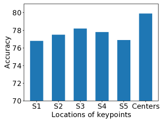
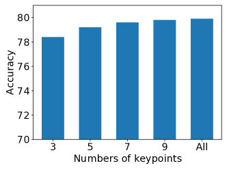
Figure 8: (a) Results for different locations of source keypoints. (b)Results for different numbers of source keypoints.

6.2.2 Ablation Studies

The ablation studies are conducted in HDA task.

Effect of target keypoints.

The keypoints are important to KPG-RL, since they are used to guide the matching. We show the results with varying keypoints by giving different numbers and samplings of labeled target domain data, in Table 2. It can be observed in Table 2 that under different numbers and samplings of labeled target domain data, our approach KPG-RL (SH) consistently outperforms the baseline Labeled-target-only, achieving positive transfer. We also find that as the number of labeled target domain data increases, the margin between the accuracy of Labeled-target-only and KPG-RL (SH) decreases. This indicates that given more labeled target domain data, the necessity of knowledge transferred from source domain becomes smaller.

Effect of source keypoints.

In the paper, the source keypoints are taken as the source class centers. To study the sensitivity to the location of source keypoints, we randomly sample one data point from each class as a keypoint to construct the source keypoints. We run the experiments with five different samplings for constructing the source keypoints (these five runs are denoted as S1, S2, S3, S4, S5, respectively). The results are reported in Fig. 8. We can see that using the class center as the keypoints achieves the best results, compared with randomly sampling one data point per class as the keypoints. This may be because the class centers are estimated using all the data of each class, and these centers can better represent each class than a randomly sampled data point of each class. We next study the sensitivity to the number of source keypoints, of which the results are reported in Fig. 8. We randomly sample 3/5/7/9 samples (keypoints) or use all the source samples (keypoints) for each class in the source domain to compute the source class centers, which are paired with labeled target samples for constructing the keypoint pairs. The results in Fig. 8 show that as the number of source keypoints increases, the accuracy gradually increases. The best result is obtained when all source samples are used to compute the class centers.

Comparison of different choices for $\bm{d}$.

Since $R_{k}^{s}$ and $R_{l}^{t}$ are in the probability simplex, it is reasonable to measure their difference by a distribution divergence/distance. The widely used distribution divergences/distances include the KL-divergence, JS-divergence, and Wasserstein distance. The KL-divergence is not symmetric, so we need to determine the order of inputs. For the Wasserstein distance, one should define the ground metric first. A possible strategy is to set the ground metric to 0 if the two keypoints are paired, otherwise 1. Such a ground metric makes the Wasserstein distance equal to the $L_{1}$-distance. In this work, $d$ is taken as the JS-divergence. We compare the performance of different choices of $d$ in the experiment of HDA on Office-31, as in Table 3.

Table 3: Results of different choices of $d$ in HDA experiment on Office-31.

Choices of $d$	A$\rightarrow$A	A$\rightarrow$D	A$\rightarrow$W	D$\rightarrow$A	D$\rightarrow$D	D$\rightarrow$W	W$\rightarrow$A	W$\rightarrow$D	W$\rightarrow$W	Avg
KL-ST	59.0	89.7	83.6	56.8	95.2	89.0	57.7	93.6	88.1	79.2
KL-TS	58.1	89.0	82.3	54.2	93.9	88.1	54.2	93.2	89.4	78.0
$L_{1}$-distance	57.4	85.8	79.0	58.0	85.8	82.9	58.4	92.6	83.6	75.9
$L_{2}$-distance	52.3	85.8	81.3	53.2	91.3	82.3	52.6	90.3	82.9	74.7
GW	42.0	71.6	70.0	41.6	71.0	69.4	42.3	71.3	70.0	61.0
JS	60.0	91.6	83.6	57.4	95.8	87.7	59.1	95.2	88.4	79.9

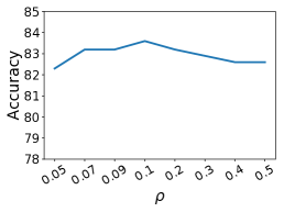
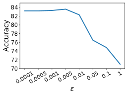
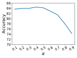
Figure 9: (a) Sensitivity of KPG-RL to hyper-parameter $\rho$. (b) Sensitivity of KPG-RL to hyper-parameter $\epsilon$. (c) Sensitivity of KPG-RL-GW to hyper-parameter $\alpha$. The results are for Closed-Set HDA task A$\rightarrow$W.

In Table 3, KL-ST and KL-TS denote the KL-divergence $KL(R_{k}^{s},R_{l}^{t})$ and $KL(R_{l}^{t},R_{k}^{s})$, respectively. GW is the Gromov-Wasserstein distance between $R_{k}^{s}$ and $R_{l}^{t}$ where the source/target cost is taken as the $L_{2}$-distance of source/target keypoints. We find that the JS-divergence achieves the best performance, compared with KL-ST, KL-TS, $L_{1}$-distance, $L_{2}$-distance, and Gromov-Wasserstein.

Sensitivity to hyper-parameters.

We show the sensitivity of our method to hyper-parameters $\rho$, $\epsilon$, and $\alpha$ in Fig. 9. $\epsilon$ is the the coefficient of entropy regularization. $\rho$ is used to set $\tau$ and $\tau^{\prime}$ for defining the relation in Eqs. (7) and (8). $\alpha$ is in the KPG-RL-GW model. The best result for $\rho$ is obtained at 0.1. For $\epsilon$, the results are relatively stable in range [0.0001,0.005]. It can be observed that the best value of $\alpha$ is 0.4 in this task, and the results are relatively stable when $\alpha$ ranges in [0.2, 0.5].

6.2.3 Open-Set Heterogeneous Domain Adaptation

We conduct open-set HDA experiments to evaluate our proposed partial-KPG-RL model. The problem setting of open-set HDA is the same as HDA, except that the unlabeled target domain data contain samples of unknown classes absent in the categories of labeled data. The goal of open-set HDA is to correctly classify the common class samples and to detect the unknown class samples. We first consider the case that the proportion $\eta$ of unknown class samples in the unlabeled target domain data is given. We then extend the approach to the case with unknown $\eta$.

Table 4: Accuracy of common class sample (OS^∗), Accuracy of unknown class sample (UNK), and their harmonic mean (HOS) on Office-31 for open-set HDA ($\eta=0.67$).

Method	A$\rightarrow$A			A$\rightarrow$D			A$\rightarrow$W			D$\rightarrow$A			D$\rightarrow$D
	OS∗	UNK	HOS	OS∗	UNK	HOS	OS∗	UNK	HOS	OS∗	UNK	HOS	OS∗	UNK	HOS
Baseline	40.0	71.0	51.2	37.3	85.3	51.9	29.1	82.7	43.0	40.0	71.0	51.2	37.3	85.3	51.9
STN	48.2	80.6	60.3	67.3	86.6	75.7	54.6	78.4	64.3	46.3	76.6	57.8	63.6	84.4	72.6
SSAN	25.4	66.7	36.8	29.1	68.4	40.8	64.5	83.1	72.7	34.6	70.6	46.4	22.7	64.1	33.6
Partial-KPG-RL	41.8	77.1	54.2	48.2	74.9	58.6	38.2	73.2	50.2	52.7	82.3	64.3	80.0	92.6	85.9
Method	D$\rightarrow$W			W$\rightarrow$A			W$\rightarrow$D			W$\rightarrow$W			Avg
	OS∗	UNK	HOS	OS∗	UNK	HOS	OS∗	UNK	HOS	OS∗	UNK	HOS	OS∗	UNK	HOS
Baseline	29.1	82.7	43.0	40.0	71.0	51.2	37.3	85.3	51.9	29.1	82.7	43.0	35.5	79.7	48.7
STN	54.6	79.2	64.6	49.9	78.4	60.4	60.0	82.6	69.5	55.5	79.2	65.2	55.6	80.7	65.6
SSAN	29.1	66.4	40.4	31.8	68.4	43.3	19.1	64.5	29.4	26.4	67.9	37.9	31.4	68.9	42.4
Partial-KPG-RL	73.6	89.2	80.7	52.7	82.7	64.4	78.2	90.9	84.1	71.8	88.3	79.2	59.7	83.5	69.1

Open-set HDA with given $\bm{\eta}$.

To apply the partial-KPG-RL model defined in Eq. (14) to open-set HDA, for each labeled target domain data, we take its corresponding source class center to construct a keypoint pair. We then resample the source domain data such that the total number of resampled source domain data and the source keypoints is $m^{\prime}=(1-\eta)n$. We define the source distribution as $\bm{p}=\frac{1-\eta}{m^{\prime}}(\sum_{j=1}^{n_{l}}\delta_{c_{j}}+\sum_{j=n_{l}+1}^{m^{\prime}}\delta_{x_{j}^{\prime}})$, where $x_{j}^{\prime}$ is a resmapled source domain sample and $c_{j}$ is the source class center corresponding to the target labeled sample $y_{j}$. The target distribution is defined as $\bm{q}=\frac{1}{n}\sum_{j=1}^{n}\delta_{y_{j}}$. The partial-KPG-RL model is conducted to transport mass from $\bm{p}$ to $\bm{q}$ with $s=1-\eta$. After transport, the $\eta$-fraction unlabeled target data receiving smallest mass from source domain are detected as unknown class and the rest unlabeled target data are taken as common class ones. Finally, we train the kernel SVM on the transported source domain data and labeled target domain data to classify the unlabeled target domain common class data.

The natural baseline for open-set HDA is the approach that rejects the $\eta$-proportion unlabeled samples with largest distance to labeled target domain data as unknown, and trains a kernel SVM on the labeled target domain data to classify common class data. We also evaluate the HDA methods STN (Yao et al., 2019) and SSAN (Li et al., 2020) in the open-set HDA task. For STN (Yao et al., 2019) and SSAN (Li et al., 2020), we reject the $\eta$-proportion unlabeled samples with lowest prediction confidence as unknown class. Table 4 reports the results. We use the open-set evaluation metrics (Bucci et al., 2020) including accuracy of common class sample (OS^∗), accuracy of unknown class sample (UNK), and their harmonic mean HOS = $2\frac{\mbox{OS}^{*}\times\mbox{UNK}}{\mbox{OS}^{*}+\mbox{UNK}}$. We can observe in Table 4 that our proposed partial-KPG-RL achieves the best results in terms of average OS^∗, UNK, and HOS, indicating that the partial-KPG-RL is effective for both classifying common class data and identifying unknown class data. Compared with the Baseline, partial-KPG-RL outperforms it by 20.4% in terms of average HOS, confirming the positive transfer achieved by our method.

Table 5: Results on Office-31 for open-set HDA with unknown $\eta$. $\hat{\eta}$ is the estimate of $\eta$ (the true $\eta=0.67$).

Method	A$\rightarrow$A			A$\rightarrow$D			A$\rightarrow$W			D$\rightarrow$A			D$\rightarrow$D
	($\hat{\eta}=0.57$)			($\hat{\eta}=0.48$)			($\hat{\eta}=0.62$)			($\hat{\eta}=0.57$)			($\hat{\eta}=0.48$)
	OS∗	UNK	HOS	OS∗	UNK	HOS	OS∗	UNK	HOS	OS∗	UNK	HOS	OS∗	UNK	HOS
Baseline	38.2	61.9	47.2	20.0	69.3	31.0	28.2	80.1	41.7	38.2	61.9	47.2	20.0	69.3	31.0
Partial-KPG-RL	49.1	70.1	57.8	61.8	59.3	60.5	54.5	73.2	62.5	59.1	73.6	65.5	83.6	66.7	74.2
Method	D$\rightarrow$W			W$\rightarrow$A			W$\rightarrow$D			W$\rightarrow$W			Avg
	($\hat{\eta}=0.62$)			($\hat{\eta}=0.57$)			($\hat{\eta}=0.48$)			($\hat{\eta}=0.62$)
	OS∗	UNK	HOS	OS∗	UNK	HOS	OS∗	UNK	HOS	OS∗	UNK	HOS	OS∗	UNK	HOS
Baseline	28.2	80.1	41.7	38.2	61.9	47.2	20.0	69.3	31.0	28.2	80.1	41.7	28.8	70.4	40.0
Partial-KPG-RL	78.2	87.4	82.6	60.9	74.5	67.0	81.8	66.7	73.5	78.2	87.0	82.4	67.5	73.2	69.5

Table 6: Average HOS of partial-KPG-RL using varying magnitude of ${\eta}$ (the unknown true value of ${\eta}$ is 0.67).

${\eta}$	0.50	0.55	0.60	0.65	0.70	0.75	0.80
Average HOS	67.2	69.2	69.9	68.7	69.2	68.5	65.5

Open-set HDA with unknown $\bm{\eta}$.

For the more practical open-set HDA setting that $\eta$ is unknown, researchers can design methods to estimate $\eta$ and then apply our method using the estimate of $\eta$, or take $\eta$ as a hyper-parameter and design methods to tune it. We directly use the positive-unlabeled learning (Bekker and Davis, 2020) method (Zeiberg et al., 2020) to estimate the fraction of common class data among the target domain unlabeled data, by taking the labeled target data as positive samples. The results of different methods for open-set HDA using the estimate $\hat{\eta}$ of $\eta$ are given in Table 5. According to Table 5, the positive transfer is achieved by our method. We can see that $\hat{\eta}$ in all tasks is lower than the true $\eta$, implying that less unknown class samples are detected. Correspondingly, the UNK value (73.2%) achieved by partial-KPG-RL using $\hat{\eta}$ in Table 5 is smaller than that (83.5%) using ${\eta}$ in Table 4. Surprisingly, the OS^∗ value (67.5%) of partial-KPG-RL in Table 5 is higher than that (59.7%) in Table 4. As a balance, the HOS value (69.5%) achieved by partial-KPG-RL using $\hat{\eta}$ is similar to the HOS value (69.1%) of partial-KPG-RL using the true $\eta$. In Table 6, we take ${\eta}$ as a hyper-parameter and show the average HOS achieved by partial-KPG-RL using varying magnitude of ${\eta}$. It is observed that the average HOS is relatively stable to ${\eta}$ in a relatively large range of $[0.55,0.75]$.

6.3 Image-to-Image Translation

The I2I translation experiments are for evaluating the proposed KPG-RL-MBP discussed in Sect. 5. We consider the “Semi-paired” I2I translation task that a large number of unpaired along with a few paired cross-domain images are given for training. We aim to leverage the paired cross-domain images to guide the desired translation. We take the paired images as keypoints and use our proposed KPG-RL-MBP to translate the source images to the target domain. To do this, we first learn the optimal transport plan based on theorem 5, and then learn the transport map through Eq. (21). The experimental details are given in Appendix.

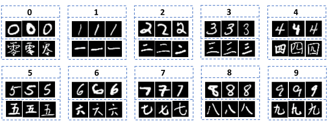
Figure 10: Examples of images from MNIST and Chinese-MNIST. In each dashed box, the first line is the digit corresponding to the images on the second and last lines. The second and last lines respectively show images from MNIST and Chinese-MNIST.

Datasets.

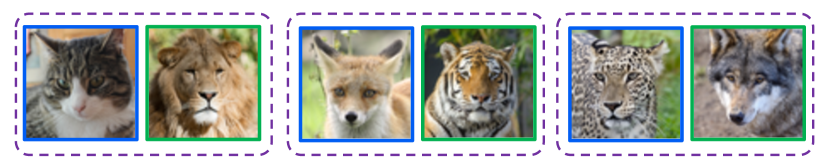
Figure 12: Annotated keypoint pairs for animal images from AFHQ dataset. Each keypoint pair is in a dashed box. In each dashed box, the source/target keypoint is with blue/green border.

The experiments are conducted on digits and natural animal images. For Digits, we take the MNIST (LeCun et al., 1998) and Chinese-MNIST datasets as source and target distributions, respectively. The MNIST and Chinese-MNIST contain the digits (from 0 to 9) in different modalities, respectively. Examples of images from MNIST and Chinese-MNIST are illustrated in Fig. 10. In experiments, we annotate 10 keypoint pairs, each corresponding to a digit, as shown in Fig. 11(a). We expect that with the guidance of the 10 keypoint pairs, the source images can be transported to the target ones representing the same digit. For Natural Animal Images, we take three species (cat, fox, leopard) of animals from AFHQ (Choi et al., 2020) as source distribution, and another three species (lion, tiger, wolf) as target distribution. We randomly choose 1000 images for each specie. To reduce the computational cost, we resize the images to 64$\times$64. Three keypoint pairs are given, as shown in Fig. 12. By the guidance of the keypoint pairs, we expect that the cat, fox, and leopard images are transported to the images of lion, tiger, and wolf, respectively.

Metrics.

We adopt two evaluation metrics, i.e., Frechet Inception Distance (FID) (Heusel et al., 2017) and Accuracy. “FID” is a commonly adopted metric in deep generative models for measuring how well the transported images resemble the target images. Lower FID indicates better image quality. The metric of “Accuracy” measures how well the source images are transported to be target images of ground-truth transported classes. For digit images, the ground-truth transported classes are defined as the digits of original source images. For animal images, the ground-truth transported classes for source images of cat, fox, and leopard are defined as lion, tiger, and wolf, respectively. Specifically, we train a classifier on the target data to recognize their class labels (i.e., digits or animal species). We then predict the class labels of the transported source images using the trained classifier, and calculate the accuracy of the predictions against corresponding ground-truth transported class labels. Higher accuracy indicates that the source images are better transported to ground-truth transported classes, and thus the guidance of keypoints is better realized.

Compared methods.

We compare the following methods, including KPG-RL-BP, KPG-RL-MBP, Cycle-GAN (w/ keypoint) (Zhu et al., 2017a), TCR (Mustafa and Mantiuk, 2020), TCR (w/ adv), WGAN-QC (w/ keypoints) (Liu et al., 2019), W2GAN (w/ keypoints) (Korotin et al., 2021), and OT-ICNN (w/ keypoints) (Makkuva et al., 2020). KPG-RL-BP and KPG-RL-MBP are respectively the BP (Eq. (20)) and our proposed MBP (Eq. (21)) based on the transport plan learned from our dual formulation of $L_{2}$-regularized KPG-RL. “Cycle-GAN (w/ keypoint)” is modified from the typical unsupervised I2I translation approach Cycle-GAN (Zhu et al., 2017a) by adding in the keypoint constraint. The keypoint constraint enforces the translated source keypoints by the generator close to the target keypoints by minimizing the MSE loss. TCR (Mustafa and Mantiuk, 2020) is the semi-supervised I2I translation approach, assuming that besides the paired images, the unpaired images are only from the source domain. In methodology, TCR introduces transformation consistency regularization to force the model’s predictions for unpaired source data to be equivariant to data transformations. Since unpaired target data are given in our setting, we additionally employ the adversarial training loss on unpaired data for TCR, which is denoted as “TCR (w/ adv)”. “WGAN-QC (w/ keypoints)”, “W2GAN (w/ keypoints)”, and “OT-ICNN (w/ keypoints)” are modified from the OT-based deep generative methods WGAN-QC (Liu et al., 2019), W2GAN (Korotin et al., 2021), and OT-ICNN (Makkuva et al., 2020) by adding the keypoint constraint to them, respectively.

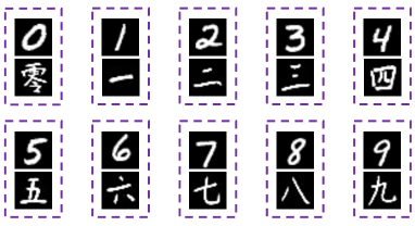
(a) Keypoints pairs

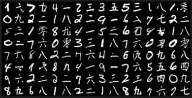
(b) Cycle-GAN (w/ keypoints)

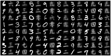
(c) KPG-RL-BP

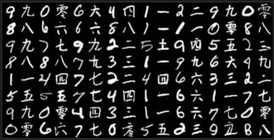
(d) KPG-RL-MBP

Figure 11: (a) Annotated keypoint pairs for digits. Each keypoint pair is in a box. (b-d) Original and transported source images by (b) Cycle-GAN (w/ keypoints), (c) KPG-RL-BP, and (d) KPG-RL-BP on digits. In (b-d), the odd columns are the source images, and their right side are the corresponding transported images.

Table 7: FID and accuracy of the transported source images. Smaller FID indicates higher quality of transported source images. Higher accuracy implies better imposing the guidance of the keypoints in transport. *WGAN-QC does not produce reasonable images in I2I translation.

Method	Digits			Natural animal images
	FID $\downarrow$	Accuracy (%) $\uparrow$		FID $\downarrow$	Accuracy (%) $\uparrow$
Cycle-GAN (w/ keypoints)	6.99	22.72		78.56	30.27
TCR	129.43	26.57		342.48	33.33
TCR (w/ adv)	6.90	36.21		74.13	32.60
*WGAN-QC (w/ keypoints)	- -	- -		- -	- -
W2GAN (w/ keypoints)	12.04	34.21		121.86	28.40
OT-ICNN (w/ keypoints)	14.37	29.12		126.43	34.67
KPG-RL-BP	157.38	74.51		285.43	60.00
KPG-RL-MBP	6.54	76.14		81.02	77.27

Results on digits for I2I translation

In Figs. 11(b), 11(c), and 11(d), we show the transported images by Cycle-GAN (w/ keypoints), KPG-RL-BP, and our proposed KPG-RL-MBP. We can observe that the transported source images by the Cycle-GAN (w/ keypoints) are clear, but there seem to be many source images incorrectly transported to be the target images of other digits. This implies that Cycle-GAN (w/ keypoints) does not well transport the source images to ground-truth transported classes (i.e., digit of the original source images). Figure 11(c) shows that most transported source images by KPG-RL-BP belong to corresponding ground-truth transported classes, but are blurry. In Fig. 11(d), it can be observed that many transported source images in even columns by KPG-RL-MBP share the same digits/class labels of the original source images in odd columns. Meanwhile, KPG-RL-MBP produces transported images with less blur than KPG-RL-BP, which is attributed to our manifold constraints $\mathcal{L}_{M}$ in Eq. (21).

We give the quantitative results in Table 7. In the left half of Table 7, we can observe that our KPG-RL-MBP achieves the highest accuracy and the lowest FID on digits among the compared approaches, indicating that our KPG-RL-MBP can better transport source images to the ground-truth transported classes and produce transported images of high quality. Note that in Table 7, WGAN-QC generates the same noisy output for all input source images, and we do not report its accuracy and FID.

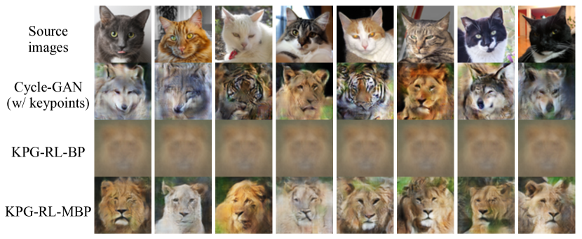
(a) Transported source images of cat.

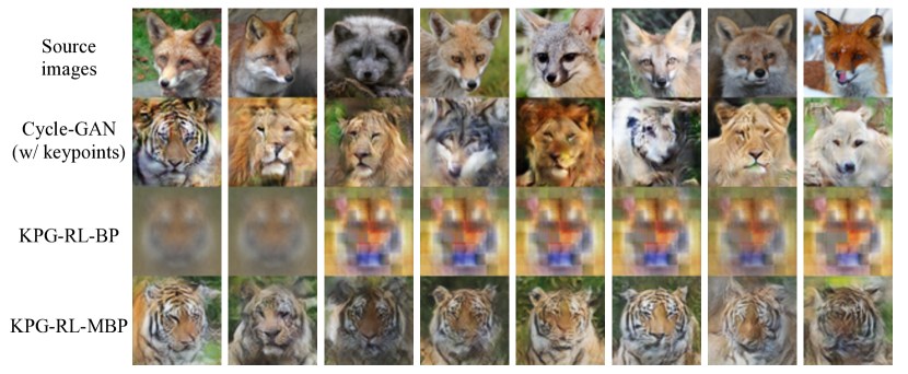
(b) Transported source images of fox.

Figure 13: Transported source images of cat and fox by Cycle-GAN (w/ keypoints), KPG-RL-BP, and KPG-RL-MBP. By the guidance of paired keypoints (see Fig. 12), the images of cat/fox are expected to be transported to images of lion/tiger.

Figure 14: Transported source images of leopard by Cycle-GAN (w/ keypoints), KPG-RL-BP, and KPG-RL-MBP. By the guidance of paired keypoints (see Fig. 12), the images of leopard are expected to be transported to images of wolf.

Results on natural animal images for I2I translation.

The results on natural animal images for I2I translation are shown in the right half of Table 7, and Figs. 13 and 14. Table 7 shows that our proposed approach KPG-RL-MBP achieves a comparable FID, compared with the other methods. The accuracy achieved by our KPG-RL-MBP is higher than that of the other compared methods by more than 17% as in Table 7. The results indicate that our approach better transport the source images to corresponding ground-truth transported classes. This is also verified by the qualitative results in Figs. 13 and 14. We explicitly model the guidance of paired keypoints to the unpaired data in KPG-RL-BP and KPG-RL-MBP, while the other approaches do not model the relation of samples to keypoints. This may account for the higher accuracy of KPG-RL-BP and KPG-RL-MBP than that of the other approaches. The KPG-RL-BP produces blurry images as in Figs. 13 and 14, because the transported images are the weighted average of target domain images according to Eq. (20). KPG-RL-MBP produces more clear images than KPG-RL-BP as shown in Figs. 13 and 14, verifying the effectiveness of the manifold barycentric projection for constraining the projected images into the target data manifold. Note that ideally, most transported images by KPG-RL-BP though should be of the ground-truth transported classes according to Eq. (20), are blurry as in Figs. 13 and 14. Hence the classifier may not recognize the transported images by KPG-RL-BP correctly. This leads to lower accuracy than KPG-RL-MBP in Table 7.

7 Conclusion

This paper proposes a novel KPG-RL model that leverages keypoints to guide the correct matching (i.e., transport plan) in OT. We devise a mask-based constraint to preserve the matching of keypoints pairs, and propose to preserve the relation of each point to the keypoints to impose the guidance of these keypoints in OT. We further propose a manifold barycentric projection to transport source images to target domain, based on the developed dual formulation of KPG-RL. The effectiveness of the proposed KPG-RL model is verified in the application of HDA and I2I translation. The keypoint-guided OT model could be possibly applied to more applications, e.g., point-set or image registration.

Appendix A: Proof of Proposition 1

Proof. For any $(i,j)\in\mathcal{K}$, from the definition of $M$, we have $M_{i,j^{\prime}}=0$ for all $j^{\prime}\neq j$ and $M_{i,j}=1$. Then, we have $\tilde{\pi}_{i,j^{\prime}}=M_{i,j^{\prime}}\pi_{i,j^{\prime}}=0$ for all $j^{\prime}\neq j$. Since $\sum_{j^{\prime}=1}^{n}\tilde{\pi}_{i,j^{\prime}}=p_{i}$, we have $\tilde{\pi}_{i,j}=p_{i}$. Similarly, we have $M_{i^{\prime},j}=0$ for all $i^{\prime}\neq i$. Then, we have $\tilde{\pi}_{i^{\prime},j}=M_{i^{\prime},j}\pi_{i^{\prime},j}=0$ for all $i^{\prime}\neq i$, and $\tilde{\pi}_{i,j}=\sum_{i^{\prime}=1}^{m}\tilde{\pi}_{i^{\prime},j}=q_{j}$. This implies that all the mass $p_{i}$ of $x_{i}$ is transported to $y_{j}$, and $y_{j}$ only receives the mass from $x_{i}$. Hence, the matching of $x_{i}$ and $y_{j}$ is preserved.

Appendix B: Deduction of Sinkhorn Iteration

The entropy-regularized model for KPG-RL is

$$\begin{split}&\min_{\pi}\langle M\odot\pi,G\rangle_{F}-\epsilon H(M\odot\pi)\\ &s.t.\hskip 5.69046pt\pi\geq 0,(M\odot\pi)\mathbbm{1}_{n}=\bm{p},(M\odot\pi)^{\top}\mathbbm{1}_{m}=\bm{q},\end{split}$$ (23)

where $H(M\odot\pi)=-\left(\langle M\odot\pi,\log(M\odot\pi)\rangle_{F}-\mathbbm{1}_{m}^{\top}(M\odot\pi)\mathbbm{1}_{n}\right)$ is the entropy of the transport plan $M\odot\pi$. The Lagrangian function is

$$\begin{split}L(\pi,\bm{f},\bm{g})=&\langle M\odot\pi,G\rangle_{F}+\epsilon\left(\langle M\odot\pi,\log(M\odot\pi)\rangle_{F}-\mathbbm{1}_{m}^{\top}(M\odot\pi)\mathbbm{1}_{n}\right)\\ &-\langle\bm{f},(M\odot\pi)\mathbbm{1}_{n}-\bm{p}\rangle_{F}-\langle\bm{g},(M\odot\pi)^{\top}\mathbbm{1}_{m}-\bm{q}\rangle_{F},\end{split}$$ (24)

where $\bm{f}\in\mathbb{R}^{m}$ and $\bm{g}\in\mathbb{R}^{n}$. The first-order conditions then yield

$$\frac{\partial L}{\partial\pi_{i,j}}=M_{i,j}G_{i,j}+\epsilon M_{i,j}\log(M_{i,j}\pi_{i,j})-M_{i,j}f_{i}-M_{i,j}g_{j}=0.$$ (25)

If $M_{i,j}=0$, $\pi_{i,j}$ could be arbitrary non-negative value, and if $M_{i,j}=1$, we have $\pi_{i,j}=e^{f_{i}/\epsilon}e^{-G_{i,j}/\epsilon}e^{g_{j}/\epsilon}$. Therefore, we have $M_{i,j}\pi_{i,j}=M_{i,j}e^{f_{i}/\epsilon}e^{-C_{i,j}/\epsilon}e^{g_{j}/\epsilon}$. The matrix form is $M\odot\pi=\mbox{diag}(\bm{u})K\mbox{diag}(\bm{v})$, where $\bm{u}=e^{\bm{f}/\epsilon},K=M\odot e^{-G/\epsilon},\mbox{ and }\bm{v}=e^{\bm{g}/\epsilon}$. The constraints are

$$\mbox{diag}(\bm{u})K\mbox{diag}(\bm{v})\mathbbm{1}_{n}=\bm{p},\hskip 11.38092pt(\mbox{diag}(\bm{u})K\mbox{diag}(\bm{v}))^{\top}\mathbbm{1}_{m}=\bm{q}.$$ (26)

Since the entries of $K$ are non-negative, Sinkhorn’s algorithm can be applied (Sinkhorn and Knopp, 1967). The iteration formulas are

$$\bm{u}^{(l+1)}=\frac{\bm{p}}{K\bm{v}^{l}},\hskip 5.69046pt\bm{v}^{(l+1)}=\frac{\bm{q}}{K^{\top}\bm{u}^{(l+1)}}.$$ (27)

The division operator used above is entry-wise.

Appendix C: Proof of Theorem 2

Proof. We denote $\ddot{\pi}=\bar{\pi}^{*}_{1:m,1:n}$ and $t=\bar{\pi}^{*}_{m+1,n+1}$. To prove Theorem 2, we first give some preparations, and then conduct the following three steps. In step 1, we show that $t=0$. In step 2, we show that $\ddot{\pi}\in\Pi^{s}(\bm{p},\bm{q};M)$ which means that $\ddot{\pi}$ is a feasible solution of problem (14) In step 3, we show that $M\odot\ddot{\pi}$ is the optimal transport plan of problem (14). We next detail these steps.

Preparations:

Since $\bar{\pi}^{*}\in\Pi(\bar{\bm{p}},\bar{\bm{q}};\bar{M})$ and $t=\bar{\pi}^{*}_{m+1,n+1}$, we have

$$\begin{split}\mathbbm{1}_{m+1}^{\top}(\bar{M}\odot\bar{\pi}^{*})\mathbbm{1}_{n+1}=&\left[\begin{matrix}\mathbbm{1}_{m}^{\top}&1\end{matrix}\right]\left(\left[\begin{matrix}M&\bm{a}\\ \bm{b}&1\end{matrix}\right]\odot\left[\begin{matrix}\ddot{\pi}&\bar{\pi}^{*}_{1:m,n+1}\\ \bar{\pi}^{*}_{m+1,1:n}&\bar{\pi}^{*}_{m+1,n+1}\end{matrix}\right]\right)\left[\begin{matrix}\mathbbm{1}_{n}\\ 1\end{matrix}\right]\\ =&\mathbbm{1}_{m}^{\top}(M\odot\ddot{\pi})\mathbbm{1}_{n}+\sum_{i=1}^{m}{a_{i}\bar{\pi}^{*}_{i,n+1}}+\sum_{j=1}^{n}{b_{j}\bar{\pi}^{*}_{m+1,j}}+t.\end{split}$$ (28)

Meanwhile, according to the constraints in $\Pi(\bar{\bm{p}},\bar{\bm{q}};\bar{M})$, we have

$$\mathbbm{1}_{m+1}^{\top}(\bar{M}\odot\bar{\pi}^{*})\mathbbm{1}_{n+1}=\mathbbm{1}_{m+1}^{\top}\bar{\bm{p}}=\|\bar{\bm{p}}\|_{1}=\|\bm{p}\|_{1}+\|\bm{q}\|_{1}-s,$$ (29)

$\sum_{i=1}^{m}{a_{i}\bar{\pi}^{*}_{i,n+1}}+t=\|\bm{p}\|_{1}-s$, and $\sum_{j=1}^{n}{b_{j}\bar{\pi}^{*}_{m+1,j}}+t=\|\bm{q}\|_{1}-s$. Combining the above equations, we have

$$\mathbbm{1}_{m}^{\top}(M\odot\ddot{\pi})\mathbbm{1}_{n}+\|\bm{p}\|_{1}+\|\bm{q}\|_{1}-2s-t=\|\bm{p}\|_{1}+\|\bm{q}\|_{1}-s.$$ (30)

Therefore,

$$\mathbbm{1}_{m}^{\top}(M\odot\ddot{\pi})\mathbbm{1}_{n}=s+t.$$ (31)

Step 1: show that $t=\bar{\pi}^{*}_{m+1,n+1}=0$.

First, we have

$$\begin{split}\langle\bar{M}\odot\bar{\pi}^{*},\bar{G}\rangle_{F}=&\sum_{i=1}^{m}\sum_{j=1}^{n}M_{i,j}\bar{\pi}^{*}_{i,j}G_{i,j}+\xi\sum_{i=1}^{m}a_{i}\bar{\pi}^{*}_{i,n+1}\\ +&\xi\sum_{j=1}^{n}b_{j}\bar{\pi}^{*}_{m+1,j}+(2\xi+A)\bar{\pi}^{*}_{m+1,n+1}\\ =&\sum_{i=1}^{m}\sum_{j=1}^{n}M_{i,j}\bar{\pi}^{*}_{i,j}G_{i,j}+\xi(\|\bm{p}\|_{1}+\|\bm{q}\|_{1}-2s-2t)+(2\xi+A)t\\ =&\sum_{i=1}^{m}\sum_{j=1}^{n}M_{i,j}\bar{\pi}^{*}_{i,j}G_{i,j}+\xi(\|\bm{p}\|_{1}+\|\bm{q}\|_{1}-2s)+At.\end{split}$$ (32)

Suppose $t=\bar{\pi}^{*}_{m+1,n+1}>0$, we next construct a solution $\gamma$ such that $\gamma_{m+1,n+1}=0$ and leads to conflict. We randomly select a set $S=\{(i,j)|\bar{\pi}^{*}_{i,j}>0,i\leq m,j\leq n,i\notin\mathcal{I},j\notin\mathcal{J}\}$ and a index pair $(i_{0},j_{0})$ satisfying the constraints of elements in $S$, such that $\sum_{(i,j)\in S}\bar{\pi}^{*}_{i,j}\leq t$ and $\sum_{(i,j)\in S}\bar{\pi}^{*}_{i,j}+\bar{\pi}^{*}_{i_{0},j_{0}}>t$. In the rest part of this section, the involved $i,j$ satisfy $i\leq m$ and $j\leq n$. Such non-empty $S$ and $(i_{0},j_{0})$ always exist, because

$$\begin{split}\mathbbm{1}_{m}^{\top}(M\odot\ddot{\pi})\mathbbm{1}_{n}=&\sum_{i=1}^{m}\sum_{j=1}^{n}{M_{i,j}\bar{\pi}^{*}_{i,j}}\\ =&\sum_{i\in\mathcal{I},j}M_{i,j}\bar{\pi}^{*}_{i,j}+\sum_{i\notin\mathcal{I},j\in\mathcal{J}}M_{i,j}\bar{\pi}^{*}_{i,j}+\sum_{i\notin\mathcal{I},j\notin\mathcal{J}}M_{i,j}\bar{\pi}^{*}_{i,j}\\ =&\sum_{i\in I}p_{i}+\sum_{i\notin\mathcal{I},j\notin\mathcal{J}}\bar{\pi}^{*}_{i,j}\mbox{ (using definition of $M$)},\end{split}$$ (33)

$\mathbbm{1}_{m}^{\top}(M\odot\ddot{\pi})\mathbbm{1}_{n}=s+t$, and $\sum_{i\in\mathcal{I}}p_{i}<s$, we have $\sum_{i\notin\mathcal{I},j\notin\mathcal{J}}\bar{\pi}^{*}_{i,j}>t$. We now move the mass of index pairs in $S$ and $(i_{0},j_{0})$ to their marginal such that a total mass of $t$ is moved. Specifically, for $(i,j)\in S$, we set $\gamma_{i,j}=0,\gamma_{i,n+1}=\bar{\pi}^{*}_{i,n+1}+\bar{\pi}^{*}_{i,j},\gamma_{m+1,j}=\bar{\pi}^{*}_{m+1,j}+\bar{\pi}^{*}_{i,j}$. For $(i_{0},j_{0})$, we set $\gamma_{i_{0},j_{0}}=\bar{\pi}^{*}_{i_{0},j_{0}}-(t-\sum_{i\notin\mathcal{I},j\notin\mathcal{J}}\bar{\pi}^{*}_{i,j}),\gamma_{i_{0},n+1}=\bar{\pi}^{*}_{i_{0},n+1}+(t-\sum_{i\notin\mathcal{I},j\notin\mathcal{J}}\bar{\pi}^{*}_{i,j}),\gamma_{m+1,j_{0}}=\bar{\pi}^{*}_{m+1,j_{0}}-(t-\sum_{i\notin\mathcal{I},j\notin\mathcal{J}}\bar{\pi}^{*}_{i,j})$. For $(i,j)\notin S$, we set $\gamma_{i,j}=\bar{\pi}^{*}_{i,j},\gamma_{i,n+1}=\bar{\pi}^{*}_{i,n+1},\gamma_{m+1,j}=\bar{\pi}^{*}_{m+1,j}$. It is easy to verify that $\gamma\in\Pi(\bar{\bm{p}},\bar{\bm{q}};\bar{M})$. Similar to Eq. (32), we have

$$\langle\bar{M}\odot\gamma,\bar{G}\rangle_{F}=\sum_{i=1}^{m}\sum_{j=1}^{n}M_{i,j}\gamma_{i,j}G_{i,j}+\xi(\|\bm{p}\|_{1}+\|\bm{q}\|_{1}-2s).$$ (34)

Using the optimality of $\bar{M}\odot\bar{\pi}^{*}$, we have

$$\langle\bar{M}\odot\gamma,\bar{G}\rangle_{F}-\langle\bar{M}\odot\bar{\pi}^{*},\bar{G}\rangle_{F}=\sum_{i=1}^{m}\sum_{j=1}^{n}M_{i,j}(\gamma_{i,j}-\bar{\pi}^{*}_{i,j})G_{i,j}-At>0.$$ (35)

From the definition of $\gamma$, we can see that $\gamma_{i,j}\leq\bar{\pi}^{*}_{i,j}$, and thus $\sum_{i=1}^{m}\sum_{j=1}^{n}M_{i,j}(\gamma_{i,j}-\bar{\pi}^{*}_{i,j})G_{i,j}\leq 0$. Hence, from Eq. (35), we have $A<0$, contradicting the assumption that $A>0$. Therefore, $t=\bar{\pi}^{*}_{m+1,n+1}=0$ holds.

Step 2: show that $\ddot{\pi}$ is a feasible solution of problem in Eq. (14).

We verify the constraints as follows.

(1) Since $\bar{\pi}^{*}\geq 0$, we have $\ddot{\pi}\geq 0$.

(2) $(\bar{M}\odot\bar{\pi}^{*})\mathbbm{1}_{n+1}=\left[\begin{matrix}M\odot\ddot{\pi}&\bm{a}\odot\bar{\pi}^{*}_{1:m,n+1}\\ \bm{b}\odot\bar{\pi}^{*}_{m+1,1:n}&0\end{matrix}\right]\left[\begin{matrix}\mathbbm{1}_{n}\\ 1\end{matrix}\right]=\left[\begin{matrix}\bm{p}\\ \|\bm{q}\|_{1}-s\end{matrix}\right]$, then $(M\odot\ddot{\pi})\mathbbm{1}_{n}+\bm{a}\odot\bar{\pi}^{*}_{1:m,n+1}=\bm{p}$, and $(M\odot\ddot{\pi})\mathbbm{1}_{n}\leq\bm{p}$.

(3) Similarly, from $(\bar{M}\odot\bar{\pi}^{*})^{\top}\mathbbm{1}_{m+1}=(\bm{q}^{\top},\|\bm{q}\|_{1}-s)^{\top}$, we have $(M\odot\ddot{\pi})^{\top}\mathbbm{1}_{m}\leq\bm{q}$.

(4) $\mathbbm{1}_{m}^{\top}(M\odot\ddot{\pi})\mathbbm{1}_{n}=s$ holds, because $t=0$ as in Step 1.

(5) $\forall i\in\mathcal{I},(\bar{M}\odot\bar{\pi}^{*})_{i,:}\mathbbm{1}_{n+1}=(M\odot\ddot{\pi})_{i,:}\mathbbm{1}_{n}+a_{i}\bar{\pi}^{*}_{i,n+1}=p_{i}$. Since $a_{i}=0$, we have $(M\odot\ddot{\pi})_{1,:}\mathbbm{1}_{n}=p_{i}$.

(6) $\forall j\in\mathcal{J},\mathbbm{1}_{m+1}^{\top}(\bar{M}\odot\bar{\pi}^{*})_{:,j}=\mathbbm{1}_{m}^{\top}(M\odot\ddot{\pi})_{:,j}+b_{j}\bar{\pi}^{*}_{m+1,j}=q_{j}$. Since $b_{j}=0$, we have $\mathbbm{1}_{m}^{\top}(M\odot\ddot{\pi})_{:,j}=q_{j}$.

Therefore, we have $\ddot{\pi}\in\Pi^{s}(\bm{p},\bm{q};M)$, and $\ddot{\pi}$ is a feasible solution of problem in Eq. (14).

Step 3: show that $M\odot\ddot{\pi}$ is the optimal transport plan of problem in Eq. (14).

Suppose there exist a transport plan $M\odot\gamma$ with $\gamma\in\Pi^{s}(\bm{p},\bm{q};M)$ such that

$$\sum_{i=1}^{m}\sum_{j=1}^{n}M_{i,j}\gamma_{i,j}G_{i,j}<\sum_{i=1}^{m}\sum_{j=1}^{n}M_{i,j}\ddot{\pi}_{i,j}G_{i,j}.$$

We construct $\bar{\gamma}$ as follows. For $i\leq m,j\leq n$, $\bar{\gamma}_{i,j}=\gamma_{i,j}$. $\bar{\gamma}_{i,n+1}=p_{i}-\sum_{j=1}^{n}\gamma_{i,j},\forall i\leq m$. $\bar{\gamma}_{m+1,j}=q_{j}-\sum_{i=1}^{n}\gamma_{i,j},\forall j\leq n$. $\bar{\gamma}_{m+1,n+1}=0$. Easily, we can verify that $\bar{\gamma}$ is in $\Pi(\bar{\bm{p}},\bar{\bm{q}};\bar{M})$. Meanwhile,

$$\begin{split}\langle\bar{M}\odot\bar{\gamma},\bar{G}\rangle_{F}=&\sum_{i=1}^{m}\sum_{j=1}^{n}M_{i,j}\gamma_{i,j}C_{i,j}+\xi(\|\bm{p}\|_{1}+\|\bm{q}\|_{1}-2s)\\ <&\sum_{i=1}^{m}\sum_{j=1}^{n}M_{i,j}\ddot{\pi}_{i,j}G_{i,j}+\xi(\|\bm{p}\|_{1}+\|\bm{q}\|_{1}-2s)=\langle\bar{M}\odot\bar{\pi}^{*},\bar{G}\rangle_{F}.\end{split}$$ (36)

This contradicts the fact that $\bar{M}\odot\bar{\pi}^{*}$ is the optimal transport plan of problem $\mbox{min}_{\bar{\pi}\in\Pi(\bar{\bm{p}},\bar{\bm{q}};\bar{M})}\langle\bar{M}\odot\bar{\pi},\bar{G}\rangle_{F}$. Therefore, $M\odot\ddot{\pi}$ is the optimal transport plan of the problem in Eq. (14).

Appendix D: Proof of Theorem 3

In Appendix D and Appendix E, for the convenience of description, we denote the mask matrix for distributions $\bm{p}$ and $\bm{q}$ as $M^{\bm{p}\bm{q}}$.

Proof. We next verify the conditions of proper metric.

(1) Show that $\mathcal{S}_{krk}(\bm{p},\bm{q})=0$ if and only if $\bm{p}=\bm{q}$.

(a) If $\bm{p}=\bm{q}$, we have $x_{i}=y_{i}$ and $p_{i}=q_{i}$ for any $i\in[m]$ (since the permutation of support points does not change the distribution). Hence, $C_{i,i}=c(x_{i},y_{i})=0$, and $C^{s}_{i,i_{u}}=c(x_{i},x_{i_{u}})=c(y_{i},y_{i_{u}})=C^{t}_{i,i_{u}},\forall i\in[m]\mbox{ and }\forall i_{u}\in\mathcal{I}$, which implies that $R^{s}_{i}=R^{t}_{i}$. Then, we have $G_{i,i}=d(R^{s}_{i},R^{t}_{i})=0$. We define $\pi$ by $\pi_{i,j}=p_{i}$ if $i=j$, otherwise 0. Obviously, $M^{\bm{p}\bm{q}}\odot\pi$ is in $\Pi(\bm{p},\bm{q};M^{\bm{p}\bm{q}})$ and $\sum_{i,j}M^{\bm{p}\bm{q}}_{i,j}\pi_{i,j}(\alpha C_{i,j}+(1-\alpha)G_{i,j})=0$. Therefore, $\mathcal{S}_{krk}(\bm{p},\bm{q})=0$.

(b) We denote $\pi^{*}$ as the optimal solution of problem (15). If $\mathcal{S}_{krk}(\bm{p},\bm{q})=0$, we have $\langle M^{\bm{p}\bm{q}}\odot\pi^{*},C\rangle_{F}=0$. This means that the KP problem $\min_{\pi\in\Pi(\bm{p},\bm{q})}\langle\pi,C\rangle_{F}=0$. Using the Proposition 2.2 in Peyré et al. (2019), we have $\bm{p}=\bm{q}$.

(2) Show that $\mathcal{S}_{krk}(\bm{p},\bm{q})=\mathcal{S}_{krk}(\bm{q},\bm{p})$.

From the definition of mask matrix in Proposition 2, we have $M^{\bm{p}\bm{q}}_{i,j}=M^{\bm{q}\bm{p}}_{j,i}$. $C$ and $G$ are symmetric because $c$ and $d$ are distances. For any $\pi\in\Pi(\bm{p},\bm{q};M^{\bm{p}\bm{q}})$, we define $\pi^{\prime}$ as $\pi^{\prime}_{i,j}=\pi_{j,i}$, and then $\pi^{\prime}\in\Pi(\bm{q},\bm{p};M^{\bm{q}\bm{p}})$. Then, we have

$$\begin{split}\mathcal{S}_{krk}(\bm{p},\bm{q})=&\min_{\pi\in\Pi(\bm{p},\bm{q};M^{\bm{p}\bm{q}})}\sum_{i,j}{M^{\bm{p}\bm{q}}_{i,j}\pi_{i,j}(\alpha C_{i,j}+(1-\alpha)G_{i,j})}\\ =&\min_{\pi\in\Pi(\bm{p},\bm{q};M^{\bm{p}\bm{q}})}\sum_{i,j}{M^{\bm{q}\bm{p}}_{j,i}\pi_{i,j}(\alpha C_{j,i}+(1-\alpha)G_{j,i})}\\ =&\min_{\pi^{\prime}\in\Pi(\bm{q},\bm{p};M^{\bm{q}\bm{p}})}\sum_{j,i}{M^{\bm{q}\bm{p}}_{j,i}\pi^{\prime}_{j,i}(\alpha C_{j,i}+(1-\alpha)G_{j,i})}\\ =&\mathcal{S}_{krk}(\bm{q},\bm{p}).\end{split}$$ (37)

(3) Show that $\mathcal{S}_{krk}(\bm{p},\bm{q})\leq\mathcal{S}_{krk}(\bm{p},\bm{r})+\mathcal{S}_{krk}(\bm{r},\bm{q})$ for any $\bm{r}=\sum_{k=1}^{m}r_{k}\delta_{z_{k}}\in\mathcal{P}_{\mathcal{I}}^{\mathcal{X}}$.

Let $M^{\bm{p}\bm{r}}\odot\pi^{\bm{p}\bm{r}}$ and $M^{\bm{r}\bm{q}}\odot\pi^{\bm{r}\bm{q}}$ be the optimal transport plans corresponding to $\mathcal{S}_{krk}(\bm{p},\bm{r})$ and $\mathcal{S}_{krk}(\bm{r},\bm{q})$, respectively. We define

$$\tilde{\gamma}=(M^{\bm{p}\bm{r}}\odot\pi^{\bm{p}\bm{r}})\mbox{diag}\left(\frac{1}{\tilde{\bm{r}}}\right)(M^{\bm{r}\bm{q}}\odot\pi^{\bm{r}\bm{q}}),$$ (38)

where the element $\tilde{r}_{j}$ of $\tilde{\bm{r}}$ is $r_{j}$ if $r_{j}>0$, and 1 otherwise. We notice that

$$\tilde{\gamma}\mathbbm{1}_{m}=(M^{\bm{p}\bm{r}}\odot\pi^{\bm{p}\bm{r}})\mbox{diag}\left(\frac{1}{\tilde{\bm{r}}}\right)\bm{r}=(M^{\bm{p}\bm{r}}\odot\pi^{\bm{p}\bm{r}})\left(\frac{\bm{r}}{\tilde{\bm{r}}}\right)=(M^{\bm{p}\bm{r}}\odot\pi^{\bm{p}\bm{r}})\tilde{\mathbbm{1}}_{m},$$ (39)

where the $j$-th location of $\tilde{\mathbbm{1}}_{m}$ is 1 if $r_{j}>0$, otherwise 0. Note that for $j$ such that $r_{j}=0$, we have $\sum_{i}(M^{\bm{p}\bm{r}}\odot\pi^{\bm{p}\bm{r}})_{i,j}=r_{j}=0$, which implies $(M^{\bm{p}\bm{r}}\odot\pi^{\bm{p}\bm{r}})_{i,j}=0$ for any $i$. Hence,

$$\tilde{\gamma}\mathbbm{1}_{m}=(M^{\bm{p}\bm{r}}\odot\pi^{\bm{p}\bm{r}})\tilde{\mathbbm{1}}_{m}=(M^{\bm{p}\bm{r}}\odot\pi^{\bm{p}\bm{r}}){\mathbbm{1}}_{m}=\bm{p}.$$ (40)

Similarity, $\tilde{\gamma}^{\top}\mathbbm{1}_{m}=\bm{q}$. Since the indexes of paired keypoints across any two distribution in $\mathcal{P}^{\mathcal{X}}_{\mathcal{I}}$ are the same, we have for any $i_{u}\in\mathcal{I}$, the $i_{u}$-th row and column of $M^{\bm{p}\bm{r}}$ and $M^{\bm{r}\bm{q}}$ are zeros except for that $M^{\bm{p}\bm{r}}_{i_{u},i_{u}}=M^{\bm{r}\bm{q}}_{i_{u},i_{u}}=1$. So the $i_{u}$-th row and column of $\tilde{\gamma}$ are zeros except for $\tilde{\gamma}_{i_{u},i_{u}}$. Then, we can write $\tilde{\gamma}_{i_{u},i_{u}}=M^{\bm{p}\bm{q}}\odot\gamma$ with $\gamma\in\mathbb{R}_{+}^{m\times m}$. Therefore, we have $\gamma\in\Pi(\bm{p},\bm{q};M^{\bm{p}\bm{q}})$. The triangle inequality then follows from

$$\begin{split}&\mathcal{S}_{krk}(\bm{p},\bm{q})=\min_{\pi\in\Pi(\bm{p},\bm{q};M^{\bm{p}\bm{q}})}\sum_{i,j}{M^{\bm{p}\bm{q}}_{i,j}\pi_{i,j}(\alpha c(x_{i},y_{j})+(1-\alpha)d(R^{s}_{i},R^{t}_{j}))}\\ \leq&\sum_{i,j}{\tilde{\gamma}_{i,j}(\alpha c(x_{i},y_{j})+(1-\alpha)d(R^{s}_{i},R^{t}_{j}))}\\ =&\sum_{i,j}(\alpha c(x_{i},y_{j})+(1-\alpha)d(R^{s}_{i},R^{t}_{j}))\sum_{k}\frac{(M^{\bm{p}\bm{r}}\odot\pi^{\bm{p}\bm{r}})_{i,k}(M^{\bm{r}\bm{q}}\odot\pi^{\bm{r}\bm{q}})_{k,j}}{\tilde{r}_{k}}\\ \end{split}$$ (41)

$$\begin{split}\leq&\sum_{i,k,j}(\alpha(c(x_{i},z_{k})+c(z_{k},y_{j}))+(1-\alpha)(d(R^{s}_{i},R^{r}_{k})+d(R^{r}_{k},R^{t}_{j}))\frac{(M^{\bm{p}\bm{r}}\odot\pi^{\bm{p}\bm{r}})_{i,k}(M^{\bm{r}\bm{q}}\odot\pi^{\bm{r}\bm{q}})_{k,j}}{\tilde{r}_{k}}\\ =&\sum_{i,k,j}(\alpha c(x_{i},z_{k})+(1-\alpha)d(R^{s}_{i},R^{r}_{k}))\frac{(M^{\bm{p}\bm{r}}\odot\pi^{\bm{p}\bm{r}})_{i,k}(M^{\bm{r}\bm{q}}\odot\pi^{\bm{r}\bm{q}})_{k,j}}{\tilde{r}_{k}}\\ +&\sum_{i,k,j}(\alpha c(z_{k},y_{j})+(1-\alpha)d(R^{r}_{k},R^{t}_{j}))\frac{(M^{\bm{p}\bm{r}}\odot\pi^{\bm{p}\bm{r}})_{i,k}(M^{\bm{r}\bm{q}}\odot\pi^{\bm{r}\bm{q}})_{k,j}}{\tilde{r}_{k}}\\ =&\sum_{i,k}(\alpha c(x_{i},z_{k})+(1-\alpha)d(R^{s}_{i},R^{r}_{k}))(M^{\bm{p}\bm{r}}\odot\pi^{\bm{p}\bm{r}})_{i,k}\\ +&\sum_{k,j}(\alpha c(z_{k},y_{j})+(1-\alpha)d(R^{r}_{k},R^{t}_{j}))(M^{\bm{r}\bm{q}}\odot\pi^{\bm{r}\bm{q}})_{k,j}\\ =&\mathcal{S}_{krk}(\bm{p},\bm{r})+\mathcal{S}_{krk}(\bm{r},\bm{q}),\end{split}$$ (42)

where $z_{k}$ is the support point of $\bm{r}$ and $R^{r}_{k}$ is the relation of $z_{k}$ to the keypoints of $\bm{r}$.

Appendix E: Proof of Theorem 4

Proof. (a) If $\bm{p}$ and $\bm{q}$ are isomorphic, for any $i\in[m]$ and any $i_{u}\in\mathcal{I}$, we have $c(x_{i},x_{i_{u}})=c^{\prime}(y_{\sigma(i)},y_{\sigma(i_{u})})=c^{\prime}(y_{\sigma(i)},y_{i_{u}})$, implying that $R_{i}^{s}=R_{\sigma(i)}^{t}$. We define $\pi$ as $\pi_{i,j}=p_{i}$ if $j=\sigma(i)$, otherwise 0. We then have

$$\begin{split}&\sum_{i,j}\alpha\Big{(}\sum_{k,l}(M^{\bm{p}\bm{q}}\odot\pi)_{i,j}(M^{\bm{p}\bm{q}}\odot\pi)_{k,l}|C^{s}_{i,k}-C^{t}_{j,l}|^{2}\Big{)}+(1-\alpha)(M^{\bm{p}\bm{q}}\odot\pi)_{i,j}G_{i,j}\\ =&\sum_{i}\Big{[}\alpha\Big{(}\sum_{k}(M^{\bm{p}\bm{q}}\odot\pi)_{i,\sigma(i)}(M^{\bm{p}\bm{q}}\odot\pi)_{k,\sigma(k)}|C^{s}_{i,k}-C^{t}_{\sigma(i),\sigma(k)}|^{2}\Big{)}\\ &\hskip 22.76228pt+(1-\alpha)(M^{\bm{p}\bm{q}}\odot\pi)_{i,\sigma(i)}G_{i,\sigma(i)}\Big{]}\\ =&\sum_{i}\Big{[}\alpha\Big{(}\sum_{k}(M^{\bm{p}\bm{q}}\odot\pi)_{i,\sigma(i)}(M^{\bm{p}\bm{q}}\odot\pi)_{k,\sigma(k)}|c(x_{i},x_{k})-c^{\prime}(x_{\sigma(i)},x_{\sigma(k)})|^{2}\Big{)}\\ &\hskip 22.76228pt+(1-\alpha)(M^{\bm{p}\bm{q}}\odot\pi)_{i,\sigma(i)}d(R^{s}_{i},R^{t}_{\sigma(i)})\Big{]}\\ =&0.\end{split}$$ (43)

This implies $\mathcal{S}_{krg}(\bm{p},\bm{q})=0$.

(b) Let $(M^{\bm{p}\bm{q}})\odot\pi^{*}$ be the optimal transport plan corresponding to $\mathcal{S}_{krg}(\bm{p},\bm{q})$. If $\mathcal{S}_{krg}(\bm{p},\bm{q})=0$, we have

$$\sum_{i,j,k,l}(M^{\bm{p}\bm{q}}\odot\pi^{*})_{i,j}(M^{\bm{p}\bm{q}}\odot\pi^{*})_{k,l}|C^{s}_{i,k}-C^{t}_{j,l}|^{2}=0.$$ (44)

This indicates that the Gromov-Wasserstein distance

$$\min_{\pi\in\Pi(\bm{p},\bm{q})}\sum_{i,j,k,l}\pi_{i,j}\pi_{k,l}|C^{s}_{i,k}-C^{t}_{j,l}|^{2}=0.$$ (45)

By virtue to Gromov-Wasserstein properties in Mémoli (2011), there exists a bijection $\sigma:[m]\longmapsto[m]$ such that $c(x_{i},x_{k})=c^{\prime}(y_{\sigma(i)},y_{\sigma(k)})$, and $p_{i}=q_{\sigma(i)}$.

Appendix F: Proof of Theorem 5

Proof. We rewrite the $L_{2}$-regularized model as

$$\begin{split}&\min_{\pi}\sum_{i,j}M_{i,j}\pi_{i,j}G_{i,j}+\epsilon\sum_{i,j}\frac{(M_{i,j}\pi_{i,j})^{2}}{p_{i}q_{j}}\\ &\mbox{s.t. }\sum_{j}M_{i,j}\pi_{i,j}=p_{i},\sum_{i}M_{i,j}\pi_{i,j}=q_{j},\pi_{i,j}\geq 0.\end{split}$$ (46)

The Lagrange function is

$$\begin{split}L(\pi,\phi,\psi)=&\sum_{i,j}M_{i,j}(G_{i,j}-\phi(x_{i})-\psi(y_{j}))\pi_{i,j}+\epsilon\sum_{i,j}\frac{M_{i,j}\pi_{i,j}^{2}}{p_{i}q_{j}}\\ +&\sum_{i}\phi(x_{i})p_{i}+\sum_{j}\psi(y_{j})q_{j},\end{split}$$ (47)

where we utilize $M_{i,j}^{2}=M_{i,j}$. Minimizing $L(\pi,\phi,\psi)$ w.r.t. $\pi$ ($\pi_{i,j}\geq 0$) is equivalent to

$$\sum_{i,j}\min_{\pi_{i,j}\geq 0}\left\{M_{i,j}(G_{i,j}-\phi(x_{i})-\psi(y_{j}))\pi_{i,j}+\epsilon\frac{M_{i,j}\pi_{i,j}^{2}}{p_{i}q_{j}}\right\}.$$ (48)

If $M_{i,j}=0$, the minimizer $\pi_{i,j}$ could be arbitrary non-negative value. If $M_{i,j}=1$, the minimizer is $\pi_{i,j}=\frac{1}{2\epsilon}(-G_{i,j}+\phi(x_{i})+\psi(y_{j}))_{+}p_{i}q_{j}$, where $a_{+}=\max\{a,0\}$. Hence, $M_{i,j}\pi_{i,j}=\frac{1}{2\epsilon}M_{i,j}(-G_{i,j}+\phi(x_{i})+\psi(y_{j}))_{+}p_{i}q_{j}.$ The dual problem is

$$\begin{split}&\max_{\phi,\psi}\min_{\pi}L(\pi,\phi,\psi)\\ =&\max_{\phi,\psi}\sum_{i}\phi(x_{i})p_{i}+\sum_{j}\psi(y_{j})q_{j}-\frac{1}{2\epsilon}\sum_{i,j}M_{i,j}(-G_{i,j}+\phi(x_{i})+\psi(y_{j}))_{+}^{2}p_{i}q_{j}\\ &+\frac{1}{4\epsilon}\sum_{i,j}M_{i,j}(-G_{i,j}+\phi(x_{i})+\psi(y_{j}))_{+}^{2}p_{i}q_{j}\\ =&\max_{\phi,\psi}\sum_{i}\phi(x_{i})p_{i}+\sum_{j}\psi(y_{j})q_{j}-\frac{1}{4\epsilon}\sum_{i,j}M_{i,j}(-G_{i,j}+\phi(x_{i})+\psi(y_{j}))_{+}^{2}p_{i}q_{j}.\end{split}$$ (49)

By the strong duality, the optimal solution $\phi^{*},\psi^{*}$ satisfies

$$(M\odot\pi^{*})_{i,j}=\frac{1}{2\epsilon}M_{i,j}(-G_{i,j}+\phi^{*}(x_{i})+\psi^{*}(y_{j}))_{+}p_{i}q_{j}.$$ (50)

Appendix G: Implementation Details for I2I Translation Experiment

The experiment consists of two steps. In the first step, we learn the potentials $\phi$ and $\psi$ based on Eq. (18) and compute the transport plan as Eq. (19). In the second step, we learn the manifold barycentric projection $T_{MBP}$ by Eq. (21).

Appendix G1: Details for the First Step

Architectures of the potentials $\bm{\phi}$ and $\bm{\psi}$ in Eq. (18).

Both ${\phi}$ and ${\psi}$ consist of a feature extractor, followed by an output head. The output head is constructed as follows: FC(1024,1024) $\rightarrow$ ReLU $\rightarrow$ FC(1024,1024) $\rightarrow$ ReLU $\rightarrow$ FC(1024,1024) $\rightarrow$ ReLU $\rightarrow$ FC(1024,1024) $\rightarrow$ ReLU $\rightarrow$ FC(1024,1), where “FC($a,b$)” is the Fully-Connected layer with input/output channel of $a$/$b$. The feature extractor is pertained and fixed. For digits, we train autoencoders for source and target images respectively, and take the encoder part of the autoencoder as the feature extractor. The architecture of the encoder part is as follows: Conv(1,32,3,1) $\rightarrow$ GN(4) $\rightarrow$ ReLU $\rightarrow$ Conv(32,64,3,2) $\rightarrow$ GN(32) $\rightarrow$ ReLU $\rightarrow$ Conv(64,128,3,2) $\rightarrow$ GN(32) $\rightarrow$ ReLU $\rightarrow$ Conv(128,256,3,2) $\rightarrow$ GN(32) $\rightarrow$ L2-Norm. The architecture of the decoder part of the autoencoder is as follows: Tconv(256,128,3,2) $\rightarrow$ GN(32) $\rightarrow$ ReLU $\rightarrow$ Tconv(128,64,3,2) $\rightarrow$ GN(32) $\rightarrow$ ReLU $\rightarrow$ Tconv(64,32,3,2) $\rightarrow$ GN(32) $\rightarrow$ ReLU $\rightarrow$ Tconv(32,1,3,1) $\rightarrow$ Sigmoid. “Conv($a,b,k,s$)” and “Tconv(a,b,k,s)” are respectively the Convolutional layer and the Transposed-Convolutional layer, where $a$ and $b$ are the input and output channel respectively, the kernel size is $k\times k$, and the stride is $s$. “GN($m$)” is the Group Normalization layer with $m$ groups. “L2-Norm” is the $L_{2}$-nomalization. For the natural animal images, the feature extractor is taken as the image encoder (“ViT-B/32”) of CLIP (Radford et al., 2021).

Training details for learning the potentials $\bm{\phi}$ and $\bm{\psi}$ in Eq. (18).

When training with Eq. (18), the optimization algorithm is Adam, the learning rate is 1e-5, and the batch size is 64. $\epsilon$ in Eq. (17) is set to 0.005.

Appendix G2: Details for the Second Step

Architectures of $\bm{T^{\prime}}$ in Eq. (21) and $\bm{D}$ in Eq. (22).

For digits, the architectures of $T^{\prime}$ is as follows: Conv(1,64,4,2) $\rightarrow$ BN $\rightarrow$ ReLU $\rightarrow$ Conv(64,128,4,2) $\rightarrow$ BN $\rightarrow$ ReLU $\rightarrow$ Conv(128, 128,3,1) $\rightarrow$ BN $\rightarrow$ ReLU $\rightarrow$ Conv(128,128,3,1) $\rightarrow$ BN $\rightarrow$ ReLU $\rightarrow$ Tconv(128,64,4,2) $\rightarrow$ BN $\rightarrow$ ReLU $\rightarrow$ Tconv(64,1,4,2) $\rightarrow$ Sigmoid, where “BN” is the Batch Normalization layer. The architectures of $D$ is as follows: Conv(1,64,4,2) $\rightarrow$ ReLU $\rightarrow$ Conv(64,128,4,2) $\rightarrow$ BN $\rightarrow$ ReLU $\rightarrow$ Conv(128,256,4,2) $\rightarrow$ BN $\rightarrow$ ReLU $\rightarrow$ Conv(256,1,3,0).

For natural animal images, we construct $T^{\prime}$ and $D$ based on the architecture of the generator and discriminator of WGAN-QC (Liu et al., 2019). The generator of WGAN-QC consists of a noise embedding layer and a resnet-based decoder. The discriminator of WGAN-QC consists of a resnet-based encoder and an FClayer. The architecture of $D$ is set to that of the discriminator of WGAN-QC. $T^{\prime}$ is constructed by stacking the resnet-based encoder and decoder. Please refer to the official code of WGAN-QC for the details of resnet-based encoder and decoder.

Training details for learning $\bm{T^{\prime}}$.

When training $T^{\prime}$ with Eq. (21), the optimization algorithm is Adam, the learning rate is 1e-4, and the batch size is 64. $\epsilon$ is set to 0.005.

References

- Alvarez-Melis and Fusi (2020) David Alvarez-Melis and Nicolo Fusi. Geometric dataset distances via optimal transport. In NeurIPS, 2020.
- Alvarez-Melis and Jaakkola (2018) David Alvarez-Melis and Tommi S Jaakkola. Gromov-wasserstein alignment of word embedding spaces. In EMNLP, 2018.
- Arjovsky et al. (2017) Martin Arjovsky, Soumith Chintala, and Léon Bottou. Wasserstein generative adversarial networks. In ICML, 2017.
- Balaji et al. (2020) Yogesh Balaji, Rama Chellappa, and Soheil Feizi. Robust optimal transport with applications in generative modeling and domain adaptation. In NeurIPS, 2020.
- Bansal et al. (2018) Aayush Bansal, Yaser Sheikh, and Deva Ramanan. Pixelnn: Example-based image synthesis. In ICLR, 2018.
- Bekker and Davis (2020) Jessa Bekker and Jesse Davis. Learning from positive and unlabeled data: A survey. ML, 109(4):719–760, 2020.
- Blondel et al. (2018) Mathieu Blondel, Vivien Seguy, and Antoine Rolet. Smooth and sparse optimal transport. In AISTATS, 2018.
- Bonneel et al. (2011) Nicolas Bonneel, Michiel Van De Panne, Sylvain Paris, and Wolfgang Heidrich. Displacement interpolation using lagrangian mass transport. In SIGGRAPH Asia, 2011.
- Bucci et al. (2020) Silvia Bucci, Mohammad Reza Loghmani, and Tatiana Tommasi. On the effectiveness of image rotation for open set domain adaptation. In ECCV, pages 422–438, 2020.
- Caffarelli and McCann (2010) Luis A Caffarelli and Robert J McCann. Free boundaries in optimal transport and monge-ampere obstacle problems. Ann Math, 171:673–730, 2010.
- Cayton (2005) Lawrence Cayton. Algorithms for manifold learning. Univ. of California at San Diego Tech. Rep, 12(1-17):1, 2005.
- Chapel et al. (2020) Laetitia Chapel, Mokhtar Z Alaya, and Gilles Gasso. Partial optimal transport with applications on positive-unlabeled learning. In NeurIPS, 2020.
- Chen et al. (2020) Ting Chen, Simon Kornblith, Mohammad Norouzi, and Geoffrey Hinton. A simple framework for contrastive learning of visual representations. In ICML, pages 1597–1607, 2020.
- Chizat et al. (2018) Lenaic Chizat, Gabriel Peyré, Bernhard Schmitzer, and François-Xavier Vialard. An interpolating distance between optimal transport and fisher–rao metrics. FoCM, 18(1):1–44, 2018.
- Choi et al. (2021) Jooyoung Choi, Sungwon Kim, Yonghyun Jeong, Youngjune Gwon, and Sungroh Yoon. Ilvr: Conditioning method for denoising diffusion probabilistic models. In ICCV, 2021.
- Choi et al. (2020) Yunjey Choi, Youngjung Uh, Jaejun Yoo, and Jung-Woo Ha. Stargan v2: Diverse image synthesis for multiple domains. In CVPR, 2020.
- Courty et al. (2017) Nicolas Courty, Rémi Flamary, Devis Tuia, and Alain Rakotomamonjy. Optimal transport for domain adaptation. IEEE Trans. PAMI, 39(9):1853–1865, 2017.
- Crum et al. (2004) William R Crum, Thomas Hartkens, and DLG Hill. Non-rigid image registration: theory and practice. Br J Radiol, 77(suppl_2):S140–S153, 2004.
- Cuturi (2013) Marco Cuturi. Sinkhorn distances: Lightspeed computation of optimal transport. In NeurIPS, 2013.
- Dessein et al. (2018) Arnaud Dessein, Nicolas Papadakis, and Jean-Luc Rouas. Regularized optimal transport and the rot mover’s distance. JMLR, 19(1):590–642, 2018.
- Donahue et al. (2014) Jeff Donahue, Yangqing Jia, Oriol Vinyals, Judy Hoffman, Ning Zhang, Eric Tzeng, and Trevor Darrell. Decaf: A deep convolutional activation feature for generic visual recognition. In ICML, 2014.
- Fang et al. (In press, 2022) Zhen Fang, Jie Lu, Feng Liu, and Guangquan Zhang. Semi-supervised heterogeneous domain adaptation: Theory and algorithms. IEEE Trans. PAMI, In press, 2022.
- Fefferman et al. (2016) Charles Fefferman, Sanjoy Mitter, and Hariharan Narayanan. Testing the manifold hypothesis. J. Amer. Math. Soc., 29(4):983–1049, 2016.
- Figalli (2010) Alessio Figalli. The optimal partial transport problem. Arch Ration Mech Anal, 195(2):533–560, 2010.
- Genevay et al. (2018) Aude Genevay, Gabriel Peyré, and Marco Cuturi. Learning generative models with sinkhorn divergences. In AISTATS, 2018.
- Gu et al. (2022) Xiang Gu, Yucheng Yang, Wei Zeng, Jian Sun, and Zongben Xu. Keypoint-guided optimal transport with applications in heterogeneous domain adaptation. In NeurIPS, 2022.
- Guittet (2002) Kevin Guittet. Extended Kantorovich norms: a tool for optimization. PhD thesis, INRIA, 2002.
- Gulrajani et al. (2017) Ishaan Gulrajani, Faruk Ahmed, Martin Arjovsky, Vincent Dumoulin, and Aaron C Courville. Improved training of wasserstein gans. In NeurIPS, 2017.
- He et al. (2016) Kaiming He, Xiangyu Zhang, Shaoqing Ren, and Jian Sun. Deep residual learning for image recognition. In CVPR, 2016.
- Heusel et al. (2017) Martin Heusel, Hubert Ramsauer, Thomas Unterthiner, Bernhard Nessler, and Sepp Hochreiter. Gans trained by a two time-scale update rule converge to a local nash equilibrium. In NeurIPS, 2017.
- Ho et al. (2017) Nhat Ho, XuanLong Nguyen, Mikhail Yurochkin, Hung Hai Bui, Viet Huynh, and Dinh Phung. Multilevel clustering via wasserstein means. In ICML, 2017.
- Huang et al. (2016) Gao Huang, Chuan Guo, Matt J Kusner, Yu Sun, Fei Sha, and Kilian Q Weinberger. Supervised word mover’s distance. In NeurIPS, 2016.
- Huynh et al. (2021) Viet Huynh, Nhat Ho, Nhan Dam, XuanLong Nguyen, Mikhail Yurochkin, Hung Bui, and Dinh Phung. On efficient multilevel clustering via wasserstein distances. JMLR, 22(1):6421–6463, 2021.
- Isola et al. (2017) Phillip Isola, Jun-Yan Zhu, Tinghui Zhou, and Alexei A Efros. Image-to-image translation with conditional adversarial networks. In CVPR, 2017.
- Kantorovich (1942) Leonid V Kantorovich. On the translocation of masses. In Dokl. Akad. Nauk. USSR (NS), 1942.
- Khosla et al. (2020) Prannay Khosla, Piotr Teterwak, Chen Wang, Aaron Sarna, Yonglong Tian, Phillip Isola, Aaron Maschinot, Ce Liu, and Dilip Krishnan. Supervised contrastive learning. In NeurIPS, 2020.
- Kim et al. (2017) Taeksoo Kim, Moonsu Cha, Hyunsoo Kim, Jung Kwon Lee, and Jiwon Kim. Learning to discover cross-domain relations with generative adversarial networks. In ICML, 2017.
- Korotin et al. (2021) Alexander Korotin, Vage Egiazarian, Arip Asadulaev, Alexander Safin, and Evgeny Burnaev. Wasserstein-2 generative networks. In ICLR, 2021.
- Kusner et al. (2015) Matt Kusner, Yu Sun, Nicholas Kolkin, and Kilian Weinberger. From word embeddings to document distances. In ICML, 2015.
- Le et al. (2021) Khang Le, Huy Nguyen, Quang M Nguyen, Tung Pham, Hung Bui, and Nhat Ho. On robust optimal transport: Computational complexity and barycenter computation. In NeurIPS, 2021.
- LeCun et al. (1998) Yann LeCun, Léon Bottou, Yoshua Bengio, and Patrick Haffner. Gradient-based learning applied to document recognition. Proceedings of the IEEE, 86(11):2278–2324, 1998.
- Lee et al. (2019) John Lee, Max Dabagia, Eva Dyer, and Christopher Rozell. Hierarchical optimal transport for multimodal distribution alignment. In NeurIPS, 2019.
- Li et al. (2020) Shuang Li, Binhui Xie, Jiashu Wu, Ying Zhao, Chi Harold Liu, and Zhengming Ding. Simultaneous semantic alignment network for heterogeneous domain adaptation. In ACM MM, pages 3866–3874, 2020.
- Liero et al. (2018) Matthias Liero, Alexander Mielke, and Giuseppe Savaré. Optimal entropy-transport problems and a new hellinger–kantorovich distance between positive measures. Invent Math, 211(3):969–1117, 2018.
- Lin et al. (2021) Chi-Heng Lin, Mehdi Azabou, and Eva L Dyer. Making transport more robust and interpretable by moving data through a small number of anchor points. In ICML, 2021.
- Lin et al. (2022) Tianyi Lin, Nhat Ho, and Michael I Jordan. On the efficiency of entropic regularized algorithms for optimal transport. JMLR, 23(137):1–42, 2022.
- Liu et al. (2019) Huidong Liu, Xianfeng Gu, and Dimitris Samaras. Wasserstein gan with quadratic transport cost. In ICCV, 2019.
- Makkuva et al. (2020) Ashok Makkuva, Amirhossein Taghvaei, Sewoong Oh, and Jason Lee. Optimal transport mapping via input convex neural networks. In ICML, 2020.
- Mémoli (2011) Facundo Mémoli. Gromov–wasserstein distances and the metric approach to object matching. FoCM, 11(4):417–487, 2011.
- Meng et al. (2021) Chenlin Meng, Yutong He, Yang Song, Jiaming Song, Jiajun Wu, Jun-Yan Zhu, and Stefano Ermon. Sdedit: Guided image synthesis and editing with stochastic differential equations. In ICLR, 2021.
- Monge (1781) Gaspard Monge. Mémoire sur la théorie des déblais et des remblais. Histoire de l’Académie Royale des Sciences de Paris, pages 666–704, 1781.
- Mozafari and Jamzad (2016) Azadeh Sadat Mozafari and Mansour Jamzad. A svm-based model-transferring method for heterogeneous domain adaptation. PR, 56:142–158, 2016.
- Mukherjee et al. (2021) Debarghya Mukherjee, Aritra Guha, Justin M Solomon, Yuekai Sun, and Mikhail Yurochkin. Outlier-robust optimal transport. In ICML, 2021.
- Mustafa and Mantiuk (2020) Aamir Mustafa and Rafał K Mantiuk. Transformation consistency regularization–a semi-supervised paradigm for image-to-image translation. In ECCV, 2020.
- Myronenko and Song (2010) Andriy Myronenko and Xubo Song. Point set registration: Coherent point drift. IEEE Trans. PAMI, 32(12):2262–2275, 2010.
- Pandey et al. (2021) Prashant Pandey, Mrigank Raman, Sumanth Varambally, and Prathosh Ap. Generalization on unseen domains via inference-time label-preserving target projections. In ICCV, 2021.
- Peyré et al. (2019) Gabriel Peyré, Marco Cuturi, et al. Computational optimal transport: With applications to data science. Foundations and Trends® in Machine Learning, 11(5-6):355–607, 2019.
- Radford et al. (2021) Alec Radford, Jong Wook Kim, Chris Hallacy, Aditya Ramesh, Gabriel Goh, Sandhini Agarwal, Girish Sastry, Amanda Askell, Pamela Mishkin, Jack Clark, et al. Learning transferable visual models from natural language supervision. In ICML, 2021.
- Reich (2013) Sebastian Reich. A nonparametric ensemble transform method for bayesian inference. SIAM JSC, 35(4):A2013–A2024, 2013.
- Russakovsky et al. (2015) Olga Russakovsky, Jia Deng, Hao Su, Jonathan Krause, Sanjeev Satheesh, Sean Ma, Zhiheng Huang, Andrej Karpathy, Aditya Khosla, Michael Bernstein, et al. Imagenet large scale visual recognition challenge. IJCV, 115(3):211–252, 2015.
- Saenko et al. (2010) Kate Saenko, Brian Kulis, Mario Fritz, and Trevor Darrell. Adapting visual category models to new domains. In ECCV, 2010.
- Saito et al. (2019) Kuniaki Saito, Donghyun Kim, Stan Sclaroff, Trevor Darrell, and Kate Saenko. Semi-supervised domain adaptation via minimax entropy. In ICCV, 2019.
- Sato et al. (2020) Ryoma Sato, Marco Cuturi, Makoto Yamada, and Hisashi Kashima. Fast and robust comparison of probability measures in heterogeneous spaces. arXiv preprint arXiv:2002.01615, 2020.
- Seguy et al. (2018) Vivien Seguy, Bharath Bhushan Damodaran, Rémi Flamary, Nicolas Courty, Antoine Rolet, and Mathieu Blondel. Large-scale optimal transport and mapping estimation. In ICLR, 2018.
- Shen and Guo (2018) Chen Shen and Yuhong Guo. Unsupervised heterogeneous domain adaptation with sparse feature transformation. In ACML, 2018.
- Sinkhorn and Knopp (1967) Richard Sinkhorn and Paul Knopp. Concerning nonnegative matrices and doubly stochastic matrices. PJM, 21(2):343–348, 1967.
- Solomon et al. (2015) Justin Solomon, Fernando De Goes, Gabriel Peyré, Marco Cuturi, Adrian Butscher, Andy Nguyen, Tao Du, and Leonidas Guibas. Convolutional wasserstein distances: Efficient optimal transportation on geometric domains. ACM ToG, 34(4):1–11, 2015.
- Sturm (2006) Karl-Theodor Sturm. On the geometry of metric measure spaces. Acta Math, 196(1):65–131, 2006.
- Tong et al. (2022) Alexander Tong, Guy Wolf, and Smita Krishnaswamy. Fixing bias in reconstruction-based anomaly detection with lipschitz discriminators. JSPS, 94(2):229–243, 2022.
- Tsai et al. (2016) Yao-Hung Hubert Tsai, Yi-Ren Yeh, and Yu-Chiang Frank Wang. Learning cross-domain landmarks for heterogeneous domain adaptation. In CVPR, 2016.
- Villani (2009) Cédric Villani. Optimal transport: old and new, volume 338. Springer, 2009.
- Wang and Mahadevan (2011) Chang Wang and Sridhar Mahadevan. Heterogeneous domain adaptation using manifold alignment. In IJCAI, 2011.
- Wang et al. (2018) Chao Wang, Haiyong Zheng, Zhibin Yu, Ziqiang Zheng, Zhaorui Gu, and Bing Zheng. Discriminative region proposal adversarial networks for high-quality image-to-image translation. In ECCV, 2018.
- Wang and Breckon (2022) Qian Wang and Toby P Breckon. Cross-domain structure preserving projection for heterogeneous domain adaptation. PR, 123:108362, 2022.
- Wu et al. (2021) Hanrui Wu, Hong Zhu, Yuguang Yan, Jiaju Wu, Yifan Zhang, and Michael K Ng. Heterogeneous domain adaptation by information capturing and distribution matching. IEEE Trans. IP, 30:6364–6376, 2021.
- Xu et al. (2020) Hongteng Xu, Dixin Luo, Ricardo Henao, Svati Shah, and Lawrence Carin. Learning autoencoders with relational regularization. In ICML, 2020.
- Yan et al. (2017) Yuguang Yan, Wen Li, Michael KP Ng, Mingkui Tan, Hanrui Wu, Huaqing Min, and Qingyao Wu. Learning discriminative correlation subspace for heterogeneous domain adaptation. In IJCAI, 2017.
- Yan et al. (2018) Yuguang Yan, Wen Li, Hanrui Wu, Huaqing Min, Mingkui Tan, and Qingyao Wu. Semi-supervised optimal transport for heterogeneous domain adaptation. In IJCAI, 2018.
- Yao et al. (2019) Yuan Yao, Yu Zhang, Xutao Li, and Yunming Ye. Heterogeneous domain adaptation via soft transfer network. In ACM MM, 2019.
- Yao et al. (2020) Yuan Yao, Yu Zhang, Xutao Li, and Yunming Ye. Discriminative distribution alignment: A unified framework for heterogeneous domain adaptation. PR, 101:107165, 2020.
- Yi et al. (2017) Zili Yi, Hao Zhang, Ping Tan, and Minglun Gong. Dualgan: Unsupervised dual learning for image-to-image translation. In CVPR, 2017.
- Yurochkin et al. (2019) Mikhail Yurochkin, Sebastian Claici, Edward Chien, Farzaneh Mirzazadeh, and Justin M Solomon. Hierarchical optimal transport for document representation. In NeurIPS, 2019.
- Zeiberg et al. (2020) Daniel Zeiberg, Shantanu Jain, and Predrag Radivojac. Fast nonparametric estimation of class proportions in the positive-unlabeled classification setting. In AAAI, 2020.
- Zhang et al. (2022) Jiying Zhang, Xi Xiao, Long-Kai Huang, Yu Rong, and Yatao Bian. Fine-tuning graph neural networks via graph topology induced optimal transport. In IJCAI, 2022.
- Zhang et al. (2020) Pan Zhang, Bo Zhang, Dong Chen, Lu Yuan, and Fang Wen. Cross-domain correspondence learning for exemplar-based image translation. In CVPR, 2020.
- Zhou et al. (2019a) Joey Tianyi Zhou, Sinno Jialin Pan, and Ivor W Tsang. A deep learning framework for hybrid heterogeneous transfer learning. AI, 275:310–328, 2019a.
- Zhou et al. (2019b) Joey Tianyi Zhou, Ivor W. Tsang, Sinno Jialin Pan, and Mingkui Tan. Multi-class heterogeneous domain adaptation. JMLR, 20(57):1–31, 2019b.
- Zhu et al. (2017a) Jun-Yan Zhu, Taesung Park, Phillip Isola, and Alexei A Efros. Unpaired image-to-image translation using cycle-consistent adversarial networks. In ICCV, 2017a.
- Zhu et al. (2017b) Jun-Yan Zhu, Richard Zhang, Deepak Pathak, Trevor Darrell, Alexei A Efros, Oliver Wang, and Eli Shechtman. Toward multimodal image-to-image translation. In NeurIPS, 2017b.