Effects of magnetic field on the evolution of energy density fluctuations

Abstract

We study the effects of a static and uniform magnetic field on the evolution of energy density fluctuations present in a medium. By numerically solving the relativistic Boltzmann-Vlasov equation within the relaxation time approximation, we explicitly show that magnetic field can affect the characteristics of energy density fluctuations at the timescale the system achieves local thermodynamic equilibrium. A detailed momentum mode analysis of fluctuations reveals that magnetic field increases the damping of mode oscillations, especially for the low momentum modes. This leads to a reduction in the ultraviolet (high momentum) cutoff of fluctuations and also slows down the dissipation of relatively low momentum fluctuation modes. We discuss the phenomenological implications of our study on various sources of fluctuations in relativistic heavy-ion collisions.

I. Introduction

The effects of magnetic field on the bulk evolution of dynamical systems have been extensively studied and found to be crucial for a proper understanding of the physical properties of the system. For example, the evolution of cosmic fluid in the early Universe has been found to be affected by a primordial magnetic field that can non-trivially modify the power spectrum of cosmic microwave background radiation (CMBR) cmbr_mag . The fluid evolution in the post-merger (ringdown) phase of a binary neutron star merger and the gravitational collapse of a homogeneous dust cllpsmag can be influenced by the magnetic field BNSmag0 ; BNSmag1 ; BNSmag2 ; BNSmag3 ; BNSmag4 modifying the strain amplitude and frequency spectrum of the gravitational waves BNSmag5 ; BNSmag6 ; BNSmag7 ; BNSmag8 . A strong magnetic field can also be generated in the participant zone in relativistic heavy-ion collisions larry ; lateTmB which can qualitatively modify the azimuthal anisotropic flow and power spectrum of the flow fluctuations of the hadrons ranjita ; tuchin0 ; KharzMHD ; ourMHD ; ourRev ; mhd1 ; mhd2 .

These systems were investigated within the relativistic magnetohydrodynamic (RMHD) framework where the medium is assumed to be in the local thermodynamic equilibrium. The observable consequences of magnetic field basically stem from the stiffening of the equation of state, which causes an increase in the sound speed in the plane perpendicular to the magnetic field and generates an additional momentum anisotropy in the fluid evolution Landau_em ; ranjita ; ourMHD ; ourRev .

However, expanding systems are naturally not in thermal equilibrium, but may gradually approach equilibrium from out-of-equilibrium initial conditions. Such scenarios have been perceived in the reheating of early Universe in the presence of a magnetic field magInfl1 ; magInfl2 , and in noncentral relativistic heavy-ion collisions where a deconfined state of Quark-Gluon-Plasma (QGP) RevQGP1 ; RevQGP2 ; RevQGP3 is formed in presence of a large magnetic field larry ; lateTmB ; tuchin1 ; tuchin2 ; BMEq . In these situations, the RMHD framework is not applicable and an out-of-equilibrium description is required to explore the evolution of the physical quantities as they approach local-equilibrium.

In general, fluctuations in physical quantities can exist at various length scales and may largely influence the dynamics of the system. In fact, fluctuations can be exploited to infer the information of a system at various time/length scales. For cosmic fluid and astrophysical systems, compared to long wavelength fluctuations, the short wavelength fluctuations (comparable to the coarse-grained length scale for hydrodynamic description) may not have any significant effect on the bulk evolution. In contrast, in heavy-ion collisions, fluctuations of short wavelengths comparable to the length scale, $\ell\sim 1$ fm, are particularly important in the description of the evolution dynamics of QGP droplet of transverse length $L\sim 10$ fm. These fluctuations are dominantly present at the initial stages of the collision hydroSim ; Schenke12 , and also during the space-time evolution (collisional and thermal/hydrodynamic fluctuations), and play an important role in the bulk hydrodynamic description of the QGP medium kapusta1 ; spal1 ; stephanov1 .¹

While these model studies of fluctuations were carried out in the absence of magnetic field, the short-lived strong magnetic field produced in nuclear collisions larry can affect mainly the “fast-evolving” short wavelength fluctuations and thereby the observables that are sensitive to fluctuations. Thus, it is important to study the impact of magnetic field on these fluctuations that can provide reliable insight on the medium properties in a model-to-data comparison ourRev ; saumia1 ; Schenke12i ; saumia2 ; ehr .²

In this work, we investigate within kinetic transport rischke1 ; rischke2 ; Ashu1 , the effects of an external magnetic field on the evolution of energy density fluctuations present in a slightly out-of-equilibrium medium of electrically charged particles. The magnetic field $B$ is considered to be static, uniform, and marginally weaker than the thermal energy or the temperature $T$ of the medium, i.e., $\sqrt{|qB|}<T$. In particular, we solve numerically the relativistic Boltzmann-Vlasov equation within the relaxation time approximation (RTA) bgk ; Anderson ; PaulR , and show that the magnetic field can affect the evolution of energy density fluctuations in the transverse direction to $B$, leading to fluctuations of completely different characteristics at the timescale at which the medium achieves local-equilibrium. We perform momentum mode analysis of the fluctuations and demonstrate that the magnetic field enhances the damping of mode oscillations. We extend the analysis to the high momentum scale of fluctuations where the nonhydrodynamic modes of RTA kinetic theory dominate PaulR0 ; heinz1 ; PaulR ; kurkela1 ; PaulR1 ; kurkela2 ; ehr and determine the ultraviolet cutoff of fluctuations above which all the higher momentum modes get suppressed while approaching local-equilibrium. We show that this cutoff decreases (i.e., the short-wavelength cutoff increases) with increasing magnetic field.

We emphasize that the analysis presented here is quite general and can be applied to any system whose constituents are electrically charged. For inclusiveness, we consider a system of charged pions and discuss the phenomenological implications on relativistic heavy-ion collisions.

This paper is organized as follows. Section II deals with a detailed description of the Boltzmann-Vlasov equation, where the underlying assumptions for solving this equation are discussed. The simulation details are given in Sec. III, and the simulation results are presented in Sec. IV. In Sec. IVA, the effects of magnetic field on the evolution of energy density fluctuations are studied with an extensive analysis of the momentum modes of fluctuations. The effects of magnetic field on the other components of energy-momentum tensor are shown in Sec. IVB. In Sec. IVC, the effects of magnetic field on a generic initial energy density profile are presented, which readily elucidate the implications of the preceding sections. The phenomenological implications of the results, especially in the context of QGP formation in relativistic heavy ion collisions are discussed in Sec. V. Finally, we conclude with a summary of the work in Sec. VI.

Throughout the study, we consider the Minkowski space-time metric as $\eta_{\mu\nu}={\rm diag}(1,-1,-1,-1)$, and work in the units $k_{B}=\hbar=c=1$. The four-position and four-momentum of particle (and anti-particle) are represented by $x^{\mu}=(t,{\bf x})$ and $k^{\mu}=(k^{0},{\bf k})$, respectively, where $k^{\mu}$ is normalized to the particle’s rest mass square as $k^{\mu}k_{\mu}=m_{0}^{2}$ giving $k^{0}=\sqrt{{\bf k}^{2}+m_{0}^{2}}$ =$E_{{}_{\bf k}}$ — the energy of particle with three-momentum ${\bf k}$.

II. Boltzmann-Vlasov Equation

To study the effects of magnetic field on the equilibration of a system, we solve the relativistic Boltzmann-Vlasov (BV) equation groot ; rischke2 :

$$k^{\mu}\partial_{\mu}f+qF^{\mu\nu}k_{\nu}\frac{\partial}{\partial k^{\mu}}f=\mathcal{C}[f,\bar{f}].$$ (1)

This provides the time evolution of the single-particle phase-space distribution function $f\equiv f(t,{\bf x},{\bf k})$ of particles with electric charge $q$. Here $F^{\mu\nu}$ is the electromagnetic field tensor whose components are treated as external fields.³ The collision integral $\mathcal{C}[f,\bar{f}]$ makes the BV equation nonlinear which cannot be solved analytically bamps1 ; transMag1 ; BMEq . We consider the linear approximation — also known as the relaxation time approximation (RTA) bgk ; Anderson ; PaulR — where the system is assumed to be slightly away from the equilibrium state such that the distribution function can be written as $f=f_{\rm eq}+\delta f$, where $f_{\rm eq}$ is the local equilibrium distribution function of the system and $\delta f\ll f_{\rm eq}$ gives the deviation from $f_{\rm eq}$.

In RTA, the collision integral can be written in the linear form as $\mathcal{C}[f,\bar{f}]$=$-\frac{k^{\mu}u_{\mu}}{\tau_{c}}\delta f$ Anderson ; Ashu1 , where $\tau_{c}$ is the relaxation time which sets a timescale for local equilibration Anderson ; PaulR , $u^{\mu}$=$\gamma(1,{\bf v})$ the four-velocity of the fluid, and $\gamma$=$(1-{\bf v}^{2})^{-1/2}$ the Lorentz factor. For anti-particles, the Boltzmann-Vlasov equation has a form similar to Eq. (1) with $(f,q)\leftrightarrow(\bar{f},-q)$ and the collision term under the RTA as $\bar{\mathcal{C}}[f,\bar{f}]$=$-\frac{k^{\mu}u_{\mu}}{\tau_{c}}\delta\bar{f}$.⁴ The collision term within RTA is constrained by the Landau matching conditions required to satisfy the net-particle four-current and energy-momentum conservations landau_k ; Anderson ; sunil2022 . These conditions are given by

$$\begin{split}u_{\mu}T^{\mu\nu}=u_{\mu}T^{\mu\nu}_{\rm eq},\\ u_{\mu}N^{\mu}=u_{\mu}N^{\mu}_{\rm eq},\end{split}$$ (2)

which should be satisfied throughout the evolution of distribution functions Anderson ; sunil2022 . Here $T^{\mu\nu}$ and $T^{\mu\nu}_{\rm eq}$ are the energy-momentum tensors of the medium corresponding to distribution functions ($f,\bar{f}$) and local equilibrium distribution functions ($f_{\rm eq},\bar{f}_{\rm eq}$), respectively. Likewise, $N^{\mu}$ and $N^{\mu}_{\rm eq}$ are the net-particle four-currents corresponding to ($f,\bar{f}$) and ($f_{\rm eq},\bar{f}_{\rm eq}$), respectively. These variables can be calculated by using the relations groot ; sunil2022

$$\begin{split}T^{\mu\nu}=\int dK~{}k^{\mu}k^{\nu}(f+\bar{f}),\\ N^{\mu}=\int dK~{}k^{\mu}(f-\bar{f}),~{}~{}~{}\end{split}$$ (3)

where $dK=d^{3}k/[(2\pi)^{3}E_{{}_{\bf k}}]$ is the Lorentz invariant momentum space integration measure. The Landau matching conditions are satisfied by the Landau-Lifshitz’s definition of four-velocity $u^{\mu}$ sunil2022 ; groot :

$$u^{\mu}=\frac{T^{\mu\nu}u_{\nu}}{u_{\rho}T^{\rho\sigma}u_{\sigma}}.$$ (4)

In this definition, the momentum density and energy flux are zero in the local rest frame of the medium.⁵

We consider a static and uniform magnetic field along $y$ direction, i.e., ${\bf B}$=$B_{0}\hat{y}$, which yields the BV equation of the form

$$E_{{}_{\bf k}}\frac{\partial f}{\partial t}+k_{x}\frac{\partial f}{\partial x}+k_{y}\frac{\partial f}{\partial y}+k_{z}\frac{\partial f}{\partial z}+qB_{0}\Big{(}k_{x}\frac{\partial f}{\partial k_{z}}-k_{z}\frac{\partial f}{\partial k_{x}}\Big{)}$$

$$=\frac{k^{\mu}u_{\mu}}{\tau_{c}}(f_{\rm eq}-f).$$ (5)

The magnetic field thus affects the distribution function in the $(k_{x},k_{z})$ plane, but has no effect in the $k_{y}$ direction. This suggest that during evolution, the magnetic field can by itself generate three-dimensional spatial anisotropies of any fluctuation present in the system. Further, in the RTA (without non-linearity), direct coupling between the fluctuation modes in the transverse ($xz$) plane and the parallel ($y$) direction is not expected. Consequently, such anisotropies can grow in the linear regime until the fluctuations decay to vanishingly small values.

Solving the integro-differential Boltzmann-Vlasov equation in (6+1)-dimensional phase-space becomes computationally quite intensive as we are interested in studying the short-wavelength fluctuations that require small lattice spacing and hence large number of lattice points. We take recourse to a tractable (3+1)-dimension equation, where we consider the evolution of distribution function $f\equiv f(t,x,k_{x},k_{z})$ for magnetic field pointing along $y$ direction. This implies a variation of $f$ in phase-space along $x$ direction and homogeneity along $y$ direction with $k_{y}=0$.⁶ Further, $f$ is taken homogeneous along spatial $z$ direction, but its variation is accounted along $k_{z}$. This allows us to study the effect of magnetic field that generates finite values of $T^{0z}$ and $T^{xz}$.⁷ For numerical simulations we rewrite the BV equations for particles and anti-particles in the dimensionless form

$$\begin{split}E_{{}_{\bf k^{\prime}}}\frac{\partial f}{\partial t^{\prime}}+k^{\prime}_{x}\frac{\partial f}{\partial x^{\prime}}+\beta_{0}\Big{(}k_{x}^{\prime}\frac{\partial f}{\partial k_{z}^{\prime}}-k_{z}^{\prime}\frac{\partial f}{\partial k_{x}^{\prime}}\Big{)}=k^{\prime\mu}u_{\mu}(f_{\rm eq}-f),\\ E_{{}_{\bf k^{\prime}}}\frac{\partial\bar{f}}{\partial t^{\prime}}+k^{\prime}_{x}\frac{\partial\bar{f}}{\partial x^{\prime}}-\beta_{0}\Big{(}k_{x}^{\prime}\frac{\partial\bar{f}}{\partial k_{z}^{\prime}}-k_{z}^{\prime}\frac{\partial\bar{f}}{\partial k_{x}^{\prime}}\Big{)}=k^{\prime\mu}u_{\mu}(\bar{f}_{\rm eq}-\bar{f}),\end{split}$$ (6)

where we have introduced the dimensionless variables $t^{\prime}$=$t/\tau_{c}$, $x^{\prime}$=$x/\tau_{c}$, ${\bf k^{\prime}}$=${\bf k}/m_{0}$ (hence $E_{{}_{\bf k^{\prime}}}$=$E_{{}_{\bf k}}/m_{0}$), with $|{\bf k}|=\sqrt{k_{x}^{2}+k_{z}^{2}}$. The term $\beta_{0}$=$|qB|\tau_{c}/m_{0}$, is dubbed as the “magnetic field parameter” which is varied to study the impact of magnetic field $B$ on the medium evolution. The two coupled differential equations in Eq. (6) are simultaneously solved numerically for complete dynamical evolution. To ensure energy-momentum and net-particle four-current conservations by the RTA collision kernel, the Landau matching conditions given in Eq. (2) are imposed, i.e., $\varepsilon=\varepsilon_{\rm eq}(T,\mu)$ and $n=n_{\rm eq}(T,\mu)$ Anderson ; sunil2022 ; spal2 ; chandro22 . The energy density $\varepsilon=u_{\mu}u_{\nu}T^{\mu\nu}$ and the net-particle density $n=u_{\mu}N^{\mu}$ can be obtained from Eq. (3). Similarly, the equilibrium energy density $\varepsilon_{\rm eq}=u_{\mu}u_{\nu}T^{\mu\nu}_{\rm eq}$ and the net-particle density $n=u_{\mu}N^{\mu}_{\rm eq}$ can be obtained from Eq. (3) by using the local-equilibrium distributions

$$f_{\rm eq}=\frac{1}{\exp{(\beta E_{{}_{\bf k}}-\alpha)}\pm 1},~{}\bar{f}_{\rm eq}=\frac{1}{\exp{(\beta E_{{}_{\bf k}}+\alpha)}\pm 1},$$ (7)

where $\pm$ refer to fermions and bosons, respectively. The associated equilibrium temperature $T=1/\beta$, chemical potential $\mu=\alpha/\beta$ are solved by using the matching conditions. It may be noted that alternative collision kernels are also available, such as the Bhatnagar-Gross-Krook (BGK) collision kernel bgk and its relativistic extensions bgk1 ; bgk2 ; rafelski1 ; rafelski2 ; pracheta that conserves net-particle four-current, and the recently proposed novel RTA novelRTA .

To generate the initial configuration of $f$ (and $\bar{f}$), the following procedure is adopted. We start with a local equilibrium state defined by a temperature $T(x^{\prime})$ that gives a local equilibrium distribution function $f_{\rm eq}$. Specifically, we consider sine-Gaussian function for temperature fluctuations which gives

$$T(x^{\prime})=T_{0}+\delta T\sin\Big{(}\frac{2\pi rx^{\prime}}{L}\Big{)}\exp(-x^{\prime 2}/2\chi^{2}),$$ (8)

where $T_{0}$ resembles the global equilibrium temperature with a corresponding distribution function $f_{0}$. $\delta T$ is the temperature fluctuation scale factor which is taken sufficiently small $\delta T$=0.01$T_{0}$. This ensures that long timescales are required to smooth out the inhomogeneities in $T(x^{\prime})$ and achieve global equilibrium in the system of total size $L$. The Gaussian width is taken to be $\chi$=$L/10$ and the “fluctuation parameter” $r$ is varied to simulate the effects of magnetic field on different wavelength fluctuations. This procedure also ensures that the spatial variations in $f_{\rm eq}$ are sufficiently localized compared to the total system size $L$.

We perturb further the local equilibrium state in the ($x^{\prime},k^{\prime}_{x},k^{\prime}_{z}$) space such that the system achieves an out-of-equilibrium state. For this purpose, we consider random fluctuations, $\delta f$, on top of $f_{\rm eq}$, which gives the initial distribution function as $f$=$f_{\rm eq}$+$\delta f$. The choice of $\delta f$ is dictated by the Landau matching conditions landau_k ; Anderson such that the initial out-of-equilibrium distribution function, $f$, gives the same net-particle number density and energy density as that given by $f_{\rm eq}$. The random fluctuation $\delta f$ is then taken as

$$\delta f=\mathcal{R}_{x^{\prime}k^{\prime}_{x}k^{\prime}_{z}}f_{\rm eq},$$ (9)

where $\mathcal{R}_{x^{\prime}k^{\prime}_{x}k^{\prime}_{z}}$ is a small random number in the ($x^{\prime},k^{\prime}_{x},k^{\prime}_{z}$) space which varies from negative to positive values. The maximum value of $|\mathcal{R}_{x^{\prime}k^{\prime}_{x}k^{\prime}_{z}}|$ is set by the RTA condition $\delta f\ll f_{\rm eq}$, which gives $|\mathcal{R}_{x^{\prime}k^{\prime}_{x}k^{\prime}_{z}}|\ll 1$. We set the maximum value of $|\mathcal{R}_{x^{\prime}k^{\prime}_{x}k^{\prime}_{z}}|=0.01$. Likewise, an initial configuration for $\bar{f}$ is also generated. Note that our final conclusions of the study are completely independent of the choices of initial fluctuations.

The fluctuations given in Eqs. (8) and (9) may be considered as an individual component out of all possible sources of non-equilibrium fluctuations present in the system, such as the initial-state or hydrodynamic fluctuations present in relativistic energy nuclear collisions hydroSim ; Schenke12 ⁸. It is therefore important to analyze the effects of magnetic field on the evolution of these fluctuations.

III. Simulation Details

The Boltzmann-Vlasov equations (6) are solved by performing numerical simulations on a lattice of dimension $1500\times 500\times 500$ with 1500 lattice points along $x^{\prime}$ direction. The spatial and momentum step sizes are chosen to be $\Delta x^{\prime}$=$\Delta k_{x}^{\prime}$=$\Delta k_{z}^{\prime}$=0.01, yielding a total system size of $L=15$ in spatial direction and $2L_{{}_{k^{\prime}}}=5$ in the momentum direction. The time step for evolution of distribution functions is taken to be $\Delta t^{\prime}$=$\Delta x^{\prime}/2$. At the initial time, the medium velocity is considered to be zero. The simulations are performed using the second-order Leapfrog method leapfrog with periodic boundary conditions along all the three directions (one space and two momentum).

With the given choice of simulation parameters, it is convenient to consider a medium of charged pions $\pi^{\pm}$ (of mass $m_{0}=m_{\pi}=140$ MeV) which is slightly away from the equilibrium state with an ambient (global equilibrium) temperature of $T_{0}=50$ MeV. The charge chemical potential $\mu_{Q}$ is varied between $0-100$ MeV, though most of our results are presented at $\mu_{Q}=100$ MeV.⁹ In the equilibrium, this pionic medium follows the Bose-Einstein distribution function.

In the study, the strength of magnetic field is constrained by the thermal energy ($\sim T$) of the medium rischke1 and taken in the marginally weak field limit $\sqrt{|qB|}<T$ transMag1 . (A large $B$ would cause Landau quantization of the energy levels in the transverse plane, which is not the interest of the present study.) In terms of the magnetic field parameter $\beta_{0}$ of Eq. (6), this condition becomes equivalent to $\beta_{0}<\tau_{c}T^{2}/m_{0}$. For the pionic medium considered at $T\simeq 50$ MeV with $\mu_{Q}=0-100$ MeV and for typical values of relaxation time $\tau_{c}\gtrsim 15$ fm rlx1 ; rlx2 , the above condition gives $\beta_{0}\lesssim 1$. Accordingly, we have taken values of $\beta_{0}=0-0.7$ in this analysis.

It may be noted that the strength of the magnetic field generated in the medium in relativistic heavy-ion collision can be estimated from the difference in the polarizations of $\Lambda$ and $\bar{\Lambda}$ hyperons ($\Delta\mathcal{P}=\mathcal{P}_{\Lambda}-\mathcal{P}_{\bar{\Lambda}}$) via $B\propto T_{f}|\Delta\mathcal{P}|$ lateTmB . For STAR measurements of $\mathcal{P}_{\Lambda}$ and $\mathcal{P}_{\bar{\Lambda}}$ in Au+Au collisions at c.m. energy $\sqrt{s_{NN}}=200$ GeV star2 , a conservative upper bound of $|qB|<2.7\times 10^{-3}m_{\pi}^{2}$ was estimated at the level of one standard deviation at a freeze-out temperature of $T_{f}=150$ MeV. Since the observed value of $|\Delta\mathcal{P}|$ is found to increase rapidly with decreasing collision energy up to $\sqrt{s_{NN}}=7.7$ GeV star1 ; star2 ; kapusLambda , the magnetic field $|qB|$ and thereby $\beta_{0}$ could also increase (see also Ref. rafelski2 , where the magnetic field was shown to increase at lower collision energy mainly due to early freeze-out time). Moreover, for three standard deviations, the upper bound on the magnetic field strength becomes about six times larger than the bound given above lateTmB .

IV. Simulation Results and Discussions

A. Energy density fluctuations

In the Boltzmann-Vlasov simulation, we solve the distribution functions of particles and anti-particles at each space-time point and calculate the “dimensionless” energy density of the system by using the relation

$$\hat{\varepsilon}(x^{\prime},t^{\prime})=\int_{-L_{k^{\prime}}}^{L_{k^{\prime}}}\int_{-L_{k^{\prime}}}^{L_{k^{\prime}}}dk_{x}^{\prime}dk_{z}^{\prime}~{}E_{{}_{\bf k^{\prime}}}(f+\bar{f}).$$ (10)

The energy density fluctuations can be obtained from

$$\delta\hat{\varepsilon}=\frac{1}{\hat{\varepsilon}_{0}}\{\hat{\varepsilon}(x^{\prime},t^{\prime})-\langle\hat{\varepsilon}(x^{\prime},t^{\prime})\rangle\},$$ (11)

where $\hat{\varepsilon}_{0}$ is the global equilibrium energy density [calculated from Eq. (10) by using ($f_{0},\bar{f}_{0}$)], and $\langle\hat{\varepsilon}(x^{\prime},t^{\prime})\rangle$ is the average of $\hat{\varepsilon}(x^{\prime},t^{\prime})$ over all lattice points at time $t^{\prime}$. For our choice of $T_{0}=50$ MeV and $\mu_{Q}=100$ MeV, one obtains $\hat{\varepsilon}_{0}\approx 2.4$.

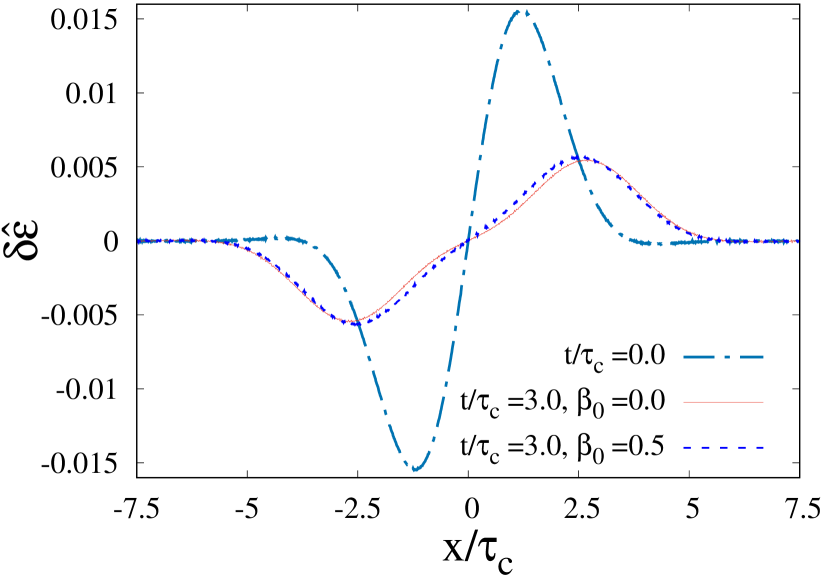
Figure 1: Energy density fluctuations at the initial time $t/\tau_{c}=0$ (dash-dotted line), and at time $t/\tau_{c}=3.0$ in the absence (solid line) and presence (dashed line) of magnetic field for the magnetic field parameter $\beta_{0}=0.5$ and the fluctuation parameter $r=2.0$.

Figure 1 shows the energy density fluctuations, $\delta\hat{\varepsilon}$, at the initial time $t/\tau_{c}=0$ (dash-dotted line), and at time $t/\tau_{c}=3.0$ in the absence (solid line) and presence (dashed line) of the magnetic field, for the magnetic field parameter $\beta_{0}=0.5$ and the fluctuation parameter $r=2.0$. Compared to the initial state, at later times the fluctuation spreads out spatially and the peak amplitudes are dominantly suppressed. The inclusion of magnetic field dampens the evolution/expansion of the underlying medium, which in turn slows down the propagation of the fluctuations in the transverse direction. As a result, the fluctuations persist with somewhat larger magnitudes and for longer duration and should influence the final observables compared to the magnetic-field-free situation.

1. Fourier modes of energy density fluctuations

In this subsection, we analyze the effects of magnetic field on energy density fluctuations in terms of momentum modes. We note that in a non-equilibrium state various momentum modes can be present, including very high momentum modes whose decay timescales are lesser than or equal to the local-equilibration timescale. Momentum of the critical mode (the mode whose decay timescale is comparable to the local-equilibration timescale) naturally sets an ultraviolet cutoff of fluctuations, above which all higher momentum modes of fluctuations are suppressed in local-equilibrium. In RTA, this cutoff is set by the local equilibrium relaxation time $\tau_{c}$, where the modes with momenta $\kappa\gtrsim\tau_{c}^{-1}$ are suppressed at the timescale of $\tau_{c}$, while modes with momenta $\kappa\lesssim\tau_{c}^{-1}$ can survive to further participate in the (hydrodynamic or RMHD) evolution. In the following analysis, we use this fact to set the momentum range (wavelength) of initial fluctuations, by accordingly varying the fluctuation parameter $r$ of Eq. (8) in the range $r\in[0.5,4.8]$.

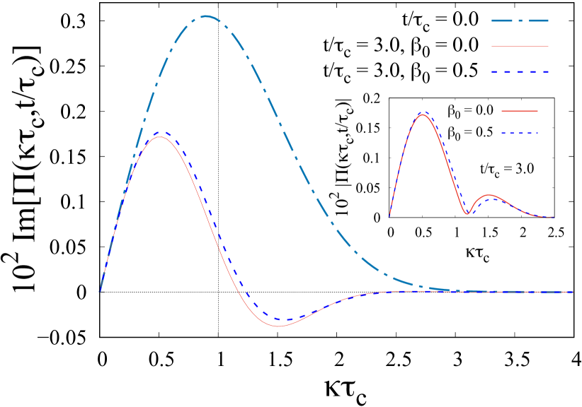
Figure 2: Momentum spectrum of energy density fluctuations at initial time (dash-dotted line), and at time $t/\tau_{c}=3.0$ in the absence (solid line) and in the presence (dashed line) of magnetic field, for the same simulation parameters as used in Fig. 1. The dotted vertical line indicates the mode at momentum $\kappa\tau_{c}=1$. In the inset, the modulus of modes versus $\kappa\tau_{c}$ is plotted for $\beta_{0}=0$ and 0.5 at $t/\tau_{c}=3.0$.

To quantify the evolution of energy density fluctuations with and without magnetic field, we perform Fourier transform from configuration $x^{\prime}$ space to the momentum $\kappa^{\prime}$ space as

$$\Pi(\kappa^{\prime},t^{\prime})=\frac{1}{L}\int_{-L/2}^{L/2}dx^{\prime}~{}\delta\hat{\varepsilon}(x^{\prime},t^{\prime})~{}e^{i\kappa^{\prime}x^{\prime}},$$ (12)

where $\kappa^{\prime}=\kappa\tau_{c}$ is the dimensionless momentum of the mode $\Pi(\kappa^{\prime},t^{\prime})$, and $\kappa$ the dimensionful momentum. Figure 2 shows the momentum spectrum (Im$[\Pi(\kappa^{\prime},t^{\prime})]$ versus $\kappa^{\prime}$) of energy density fluctuations at the initial time (dash-dotted line), and at $t/\tau_{c}=3.0$ in the absence (solid line) and in the presence (dashed line) of magnetic field, for the same simulation parameters as used in Fig. 1. At the initial time $t=0$, the peak momentum of the spectrum at $\kappa_{p}\tau_{c}=0.88$ corresponds to the most dominant mode; the magnitude and position of the peak depends on the fluctuation parameter $r$ of Eq. (8). In the inset of Fig. 2, the modulus of modes, $|\Pi(\kappa^{\prime},t^{\prime})|$, versus $\kappa\tau_{c}$ is plotted for $\beta_{0}=0$ and 0.5 at $t/\tau_{c}=3.0$.

The modulus of modes, $|\Pi(\kappa^{\prime},t^{\prime})|$, quantify the strength of fluctuations present in the system, thus as the fluctuations evolve and damp, each mode Im$[\Pi(\kappa^{\prime},t^{\prime})]$ would decrease with increasing time. Since the high momentum modes decay faster compared to the low ones, the peak of the spectrum shifts towards lower momenta at later times as can be seen at $t/\tau_{c}=3.0$. Moreover, certain higher momentum modes in the spectrum become negative, which indicates that these modes are not just decaying but also performing oscillations over time; see Fig. 3 for such damped harmonic oscillations of various modes present in the spectrum.

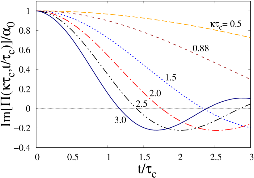
Figure 3: Damped harmonic oscillations of various non-zero modes present in the spectrum of Fig. 2 (without magnetic field). Each mode is normalized with its initial value $\alpha_{0}$ (at $t/\tau_{c}=0$) and marked with corresponding momentum $\kappa\tau_{c}$.

In Fig. 2 we also present the momentum spectrum in presence of magnetic field at time $t/\tau_{c}=3.0$ (dashed line). The magnetic field clearly affects the entire spectrum of fluctuations, retaining to some extent the strength of the initial fluctuations in the low momentum regime ($\kappa\tau_{c}\lesssim 1.2$), while suppressing the modulus of higher momentum modes relative to $B=0$ situation; see the inset of Fig. 2. This leads to characteristic change in the energy density fluctuations during the evolution towards equilibrium. Later, we have shown that magnetic field increases damping coefficient of mode oscillations causing such characteristic changes in the fluctuations.

To determine in which momentum regime the fluctuation modes are strongly affected by the magnetic field at a given time, we display in Fig. 4 the momentum spectrum for the difference of modes with and without magnetic field at time $t/\tau_{c}=3.0$. At the starting time of $t=0$, the momentum spectrum, with and without $B$, are identical. Subsequently, at later times, the magnetic field is found to influence various modes differently leading to such a structure. The maximum difference, corresponding to the peak position, occurs at a momentum $\kappa\tau_{c}\simeq 1.0$ which is larger than the peak-position momentum ($\kappa\tau_{c}\simeq 0.5$) in Fig. 2. This implies that at any instant, the magnetic field affects quantitatively more the evolution of higher momentum modes of fluctuations as these fast modes experience stronger Lorentz force (along $z^{\prime}$ direction).

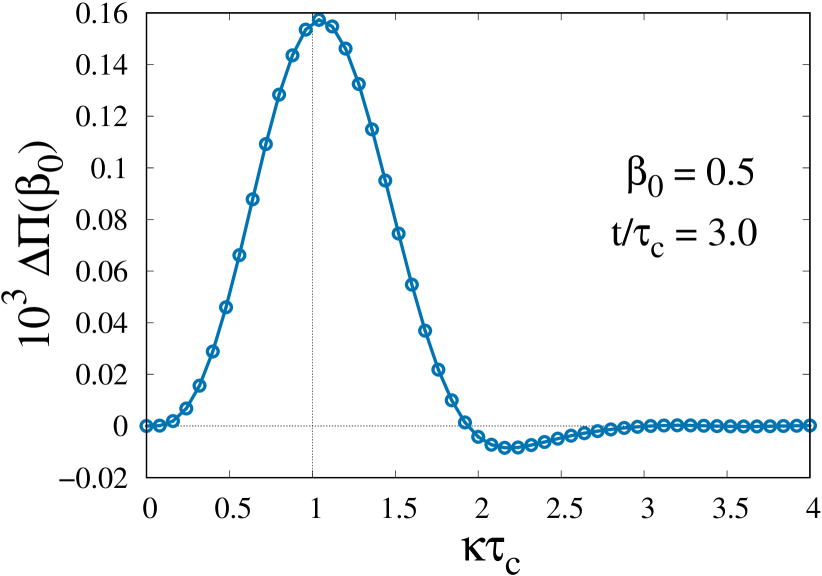
Figure 4: Momentum spectrum of difference of modes with and without magnetic field, $\Delta\Pi(\beta_{0})={\rm Im}[\Pi(\beta_{0})]-{\rm Im}[\Pi(0)]$, at time $t/\tau_{c}=3.0$ for the same simulation parameter as used in Fig. 2.

For further analysis we focus on the time evolution of the most dominant mode of energy density fluctuations. Figure 5(a) shows the time evolution of Im$[\Pi(\kappa^{\prime}_{p},t^{\prime})]$ for the dominant mode for $\kappa^{\prime}_{p}=\kappa_{p}\tau_{c}=0.88$ (corresponding to fluctuation parameter $r=2.0$) in the absence (solid line) and presence (dashed line) of magnetic field. It is clear that the effect of magnetic field becomes noticeable at times $t/\tau_{c}\gtrsim 1$ that enforces a higher magnitude in the fluctuation strength at early times followed by a gradual increase in the damping of the oscillating modes (as shown in the inset). In Fig. 5(b), we also show the the evolution of a high momentum mode $\kappa_{p}\tau_{c}=2.0$ (for $r=4.8$). This high momentum (short wavelength) mode is strongly suppressed and quickly damped in presence of magnetic field.

Figure 5: Time evolution of the most dominant mode of energy density fluctuations (a) for $\kappa_{p}\tau_{c}=0.88$ (corresponding to fluctuation parameter $r=2.0$) and (b) for $\kappa_{p}\tau_{c}=2.0$ (for $r=4.8$). The results are in the absence (solid line) and presence (dashed line) of magnetic field. Insets show the mode evolution for a longer time.

The above results demonstrate that magnetic field can affect the evolution of energy density fluctuations in the transverse plane at the timescale $t/\tau_{c}\sim 1$. Consequently, the characteristics of fluctuations in three dimensional physical space can get modified, which may generate additional spatial anisotropies. For precise quantification of the growth of these anisotropies due to magnetic field, it is necessary to perform a full (6+1)-dimensional phase-space simulation. Nevertheless, in the present (3+1)D evolution, the relation between the dominant modes of fluctuations with and without magnetic field can provide some crucial insight about this growth.

As mentioned above and evident from Figs. 3 and 5, the time evolution of ${\rm Im}[\Pi(\kappa^{\prime}_{p},t^{\prime})]$ can be best fitted with the damped harmonic oscillator function:

$$\text{Im}[\Pi(\kappa^{\prime}_{p},t^{\prime})]=\alpha_{0}\cos(\omega t^{\prime}-\phi)\exp(-\gamma_{m}t^{\prime}).$$ (13)

Here $\alpha_{0}\equiv\alpha_{0}(\kappa^{\prime}_{p})$ is the amplitude scale factor of the oscillator, $\omega\equiv\omega(\kappa^{\prime}_{p})$ the dimensionless angular frequency, $\phi\equiv\phi(\kappa^{\prime}_{p})$ the phase, and $\gamma_{m}\equiv\gamma_{m}(\kappa^{\prime}_{p})$ the dimensionless damping coefficient. We found that magnetic field has an insignificant effect on the oscillatory factor $\alpha_{0}\cos(\omega t^{\prime}-\phi)$, but increases the damping coefficient $\gamma_{m}$, and further, $\omega$ is always greater than $\gamma_{m}$ — representing an underdamped oscillator. This yields a relation between the fluctuation modes with and without $B$ as

$$\text{Im}[\Pi(\beta_{0})]\approx\text{Im}[\Pi(0)]\exp[-\delta\gamma_{m}\gamma_{m}(0)t^{\prime}],$$ (14)

where $\delta\gamma_{m}$=$[\gamma_{m}(\beta_{0})$$-$$\gamma_{m}(0)]/\gamma_{m}(0)$ is the fractional change in the damping coefficient by the magnetic field, which is completely independent of the initial magnitude of energy density fluctuations. The decay of the modes in presence of $B$ can be then conveniently determined by $\delta\gamma_{m}$.

Figure 6: Variation of “dimensionless decay timescale” $\gamma_{m}^{-1}$ of mode with peak-momentum $\kappa_{p}\tau_{c}$ for different values of magnetic parameter $\beta_{0}$.

Note that $\gamma_{m}^{-1}\tau_{c}$ sets a decay timescale of the mode, which can also be identified as the “relaxation time” of the particular mode. Figure 6 shows the variation of the “dimensionless decay timescale” $\gamma_{m}^{-1}$ of mode with peak-momentum $\kappa_{p}\tau_{c}$ for different values of magnetic field parameter $\beta_{0}$. The values of momentum in the range $\kappa_{p}\tau_{c}\in[0.64,2.0]$ are obtained by varying the fluctuation parameter between $r\in[0.5,4.8]$. In general, for any value of $\beta_{0}$, the decay timescale $\gamma_{m}^{-1}$ exhibits a decreasing trend with increasing $\kappa_{p}\tau_{c}$ as the higher momentum modes decay fast. Stronger magnetic field in the medium, i.e. with increasing $\beta_{0}$, reduces the decay timescale of especially the slow modes that actually experience magnetic force for a longer duration — inspite of higher momentum modes are largely influenced (quantitatively) by the magnetic field at any instant of time (see Fig. 4).

Each curve in Fig. 6, corresponding to a $\beta_{0}$ value, can be best fitted with a power law scaling $\gamma_{m}^{-1}$=$s_{0}(\kappa_{p}\tau_{c})^{-s_{1}}$+$s_{2}$. The mode that has a decay timescale comparable to the local-equilibration timescale of the system can be identified with a momentum cutoff $\kappa_{c}\tau_{c}$ above which all the higher momentum modes are suppressed. In other words, it resembles a “dimensionless” wavelength cutoff $\lambda^{*}_{c}=\lambda_{c}/\tau_{c}$ below which any inhomogeneity in the energy density is suppressed. This cutoff can be determined by putting $\gamma_{m}^{-1}=1$ in the above power law scaling. Figure 7 illustrates the qualitative growth of the wavelength cutoff, $\lambda^{*}_{c}(\beta_{0})$, with the magnetic field parameter $\beta_{0}$; the value of $\lambda_{c}(\beta_{0}=0)$ turns out to be about $2.5\tau_{c}$. Note that $\lambda_{c}(\beta_{0})$ is equivalent to the coarse-grained length scale inherent in the hydrodynamic description for medium evolution. The above analysis indicates that magnetic field suppresses the short wavelength fluctuations up to a larger wavelength (as compared to $B=0$) resulting in a smoother coarse-grained structure of the hydrodynamic variables.

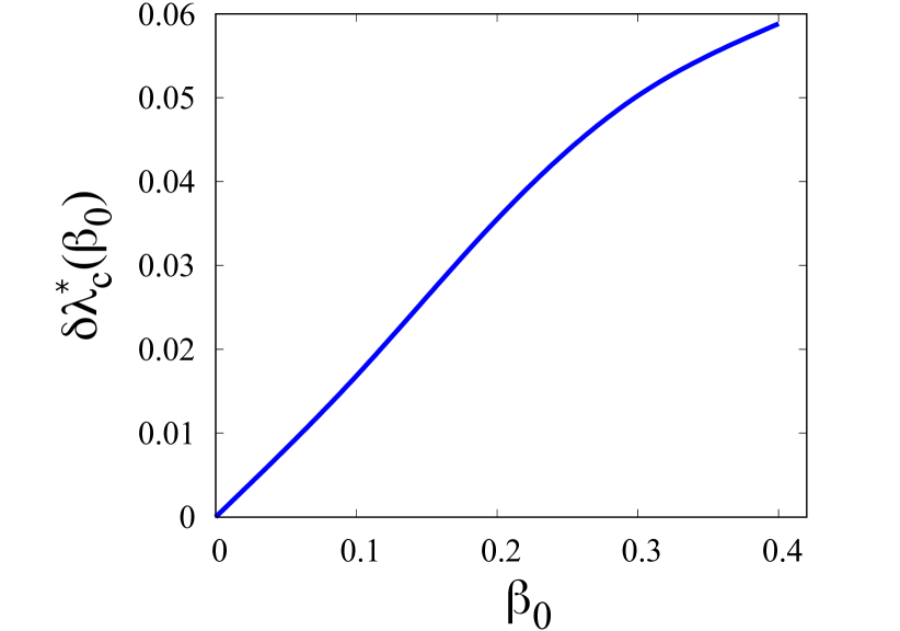
Figure 7: Magnetic field parameter $\beta_{0}$ dependence of the fractional change of wavelength cutoff $\delta\lambda^{*}_{c}(\beta_{0})$=$[\lambda^{*}_{c}(\beta_{0})-\lambda^{*}_{c}(0)]/\lambda^{*}_{c}(0)$. The bending in the curve at $\beta_{0}>0.3$ is due to the simulations and fitting procedures performed in a limited range of $\kappa_{p}\tau_{c}$.

Given that $\delta\gamma_{m}$ is enhanced more towards the lower momentum modes (see Fig. 6), we can also obtain a power law scaling behavior of $\delta\gamma_{m}$ with $\kappa_{p}\tau_{c}$ and $\beta_{0}$ (as found for $\gamma_{m}^{-1}$), namely:

$$\delta\gamma_{m}\approx\beta_{0}^{2}\left[2(\kappa_{p}\tau_{c})^{-(0.03/\beta_{0}+2)}-0.5\right].$$ (15)

This relation is completely independent of the choice of initial energy density fluctuations, and perfectly valid in the above mentioned range of $\kappa_{p}\tau_{c}$. From the above relation one can determine the fractional change in the modes, generated by the magnetic field, by using the expression $\delta\Pi=({\rm Im}[\Pi(\beta_{0})]$$-$${\rm Im}[\Pi(0)])/{\rm Im}[\Pi(0)]$. Although the damping coefficient of modes and effects of magnetic field would be quite different in three dimensional physical space, $\delta\Pi$ may be valid in that case as well. Hence, using Eqs. (14) and (15), $\delta\Pi$ provides a measure of spatial anisotropies in the energy density solely generated by the magnetic field.

B. Evolution of $\hat{T}^{\mu\nu}$ and dependence on $\mu_{Q}$

In the previous subsection, the effects of magnetic field on the evolution of energy density fluctuations ($\delta\hat{\varepsilon}=\delta\hat{T}^{00}$) have been studied and found to increase the damping coefficient of mode oscillations. In this subsection, we shall explore magnetic effects on the other components of energy-momentum tensor $\hat{T}^{\mu\nu}$ which is calculated by using Eq. (3) and performing the momentum integrals as done in Eq. (10). The spatial variation of the energy-momentum tensor components, $\hat{T}^{0x}$, $\hat{T}^{0z}$, $\hat{T}^{xz}$, and ($\hat{T}^{xx}-\hat{T}^{zz}$), is shown in Fig. 8 at time $t/\tau_{c}=3.0$ in the absence (solid line) and in the presence (dashed line) of magnetic field, for the same simulation parameters as used in Fig. 1. The variation of $\hat{T}^{0x}$ arises due to the spatial gradients present in the energy density fluctuations as shown in Fig. 1. It is clear from Fig. 8 that the magnetic field suppresses $\hat{T}^{0x}$, which essentially leads to the increase in the damping coefficient of the mode oscillations (as shown previously). The most appreciable effects of magnetic field involve the $z$-components, namely $\hat{T}^{0z}$ and $\hat{T}^{xz}$, which become rather large compared to vanishingly small values for $B=0$. Such a behavior can be traced to the Lorentz force exerted by the magnetic field that acts along $z^{\prime}$ direction on the medium evolving along $x^{\prime}$. The magnetic field is seen to also suppress substantially the magnitude of ($\hat{T}^{xx}-\hat{T}^{zz}$).

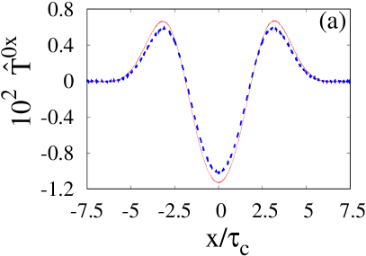
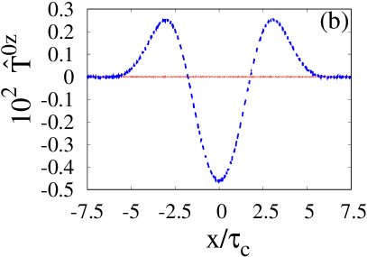
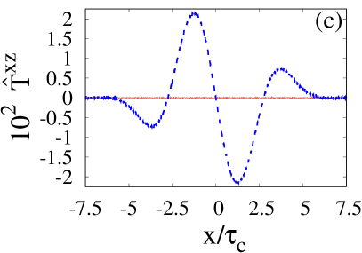
Figure 8: Spatial variation of the components of energy-momentum tensor (a) $\hat{T}^{0x}$ (b) $\hat{T}^{0z}$ (c) $\hat{T}^{xz}$ and (d) ($\hat{T}^{xx}-\hat{T}^{zz}$) at a time $t/\tau_{c}=3.0$ in the absence (solid line) and presence (dashed line) of the magnetic field for the same simulation parameters as used in Fig. 1.

It is important to comment on the effects of charge chemical potential $\mu_{Q}$ on the characteristic change seen for the components of $\hat{T}^{\mu\nu}$ and, in particular, on the energy density fluctuations in the presence of $B$. At $\mu_{Q}=0$ (when the net-electric charge density $\hat{n}=\hat{n}_{+}-\hat{n}_{-}=0$ due to identical particle and anti-particle number densities), the equal and opposite Lorentz force exerted by the magnetic field along $z^{\prime}$ direction on the positive and negatively charged particles causes $\hat{T}^{0z}$ and $\hat{T}^{xz}$ to vanish throughout their evolution. Only at finite $\mu_{Q}$, the magnitude of $\hat{T}^{0z}$ and $\hat{T}^{xz}$ become non-zero in presence of magnetic field due to net-electric charge density imbalance (as seen in Fig. 8). This also suggests, that irrespective of the value of $\mu_{Q}$, a finite $B$ will affect solely the magnitude of the momentum density $\hat{T}^{0x}$ and its accompanied energy density fluctuations $\delta\hat{\varepsilon}$. Consequently, the earlier discussed scaling of $\delta\gamma_{m}$ for a given $\beta_{0}$ will remain unaltered which we have verified for a range of $\mu_{Q}/T_{0}=0-2.0$ at a fixed equilibrium temperature $T_{0}$.

C. Fluctuations with multiple modes

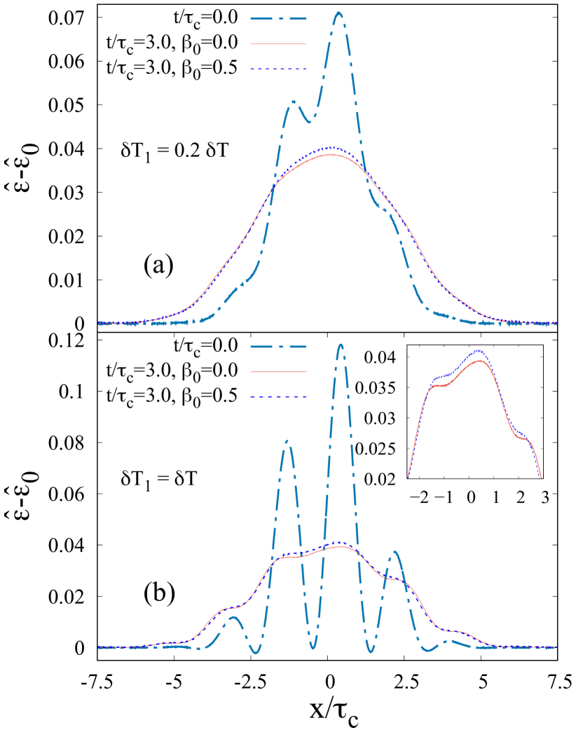
Figure 9: The energy density fluctuations, $(\hat{\varepsilon}-\hat{\varepsilon}_{0})$, at the initial time (dash-dotted lines) and at time $t/\tau_{c}=3.0$ in the absence (solid lines) and presence (dashed lines) of the magnetic field with $\beta_{0}=0.5$. The result are for mode mixing parameter (a) $\delta T_{1}=0.2\delta T$ and (b) $\delta T_{1}=\delta T$, where $\delta T=0.01T_{0}$. It is clear from (a) and inset of (b) that in presence of $B$, the energy density profile is smoother and has larger peak value as compared to $B=0$.

To illustrate the effects of magnetic field on the energy density fluctuations having more than one initial dominant mode, we consider fluctuations of the form

$$\begin{split}T(x^{\prime})=T_{0}+\Big{[}\delta T\cos\Big{(}\frac{2\pi r_{1}x^{\prime}}{L}\Big{)}+\delta T_{1}\sin\Big{(}\frac{2\pi r_{2}x^{\prime}}{L}\Big{)}\Big{]}\\ \times\exp(-x^{\prime 2}/2\chi^{2}),~{}~{}~{}~{}~{}~{}~{}~{}~{}~{}~{}~{}~{}~{}~{}~{}~{}~{}~{}~{}~{}~{}~{}~{}~{}~{}~{}~{}~{}\end{split}$$ (16)

where the mode mixing parameter $\delta T_{1}$ is varied between zero and $\delta T$ to generate different energy density fluctuations of different amplitudes. For the present study, we have taken $r_{1}=0.5$ and $r_{2}=8.0$ which allows the generation of a low and a very high momentum mode, respectively. The choice of sine and cosine functions invokes some arbitrariness (such as an asymmetry about $x^{\prime}=0$) resembling to some extent a general form for energy density fluctuations present in a physical system, for example, the initial-state fluctuations in the Glauber model Loizides:2017ack or in the gluon saturation model cgc as commonly employed for initial conditions in the modeling of relativistic heavy-ion collisions. The other simulation parameters are the same as taken previously. Figure 9 shows spatial dependence for the evolution of the energy density fluctuations, $(\hat{\varepsilon}-\hat{\varepsilon}_{0})$. The results are for a relatively small mode mixing $\delta T_{1}=0.2\delta T$ as shown in Fig. 9(a) and for maximal mixing $\delta T_{1}=\delta T$ as shown in Fig. 9(b). The initial energy density profile (dash-dotted lines) becomes rather smooth at a later time of $t/\tau=3.0$ (solid and dashed lines). This arises as the fluctuations of wavelengths shorter than the cutoff $\lambda^{*}_{c}$ are dominantly suppressed at times $t/\tau_{c}\gtrsim 1$. In presence of magnetic field, at $t/\tau=3.0$ (dashed lines), the energy density profile becomes slightly smoother and has a larger peak value as compared to $B=0$ (solid lines); see inset of Fig. 9(b). This smoothening is essentially caused by the enhanced suppression of the short wavelength (high momentum) modes, whereas the larger peak is due to slow dissipation of long wavelength (low momentum) fluctuations at early times (as discussed in Fig. 5).

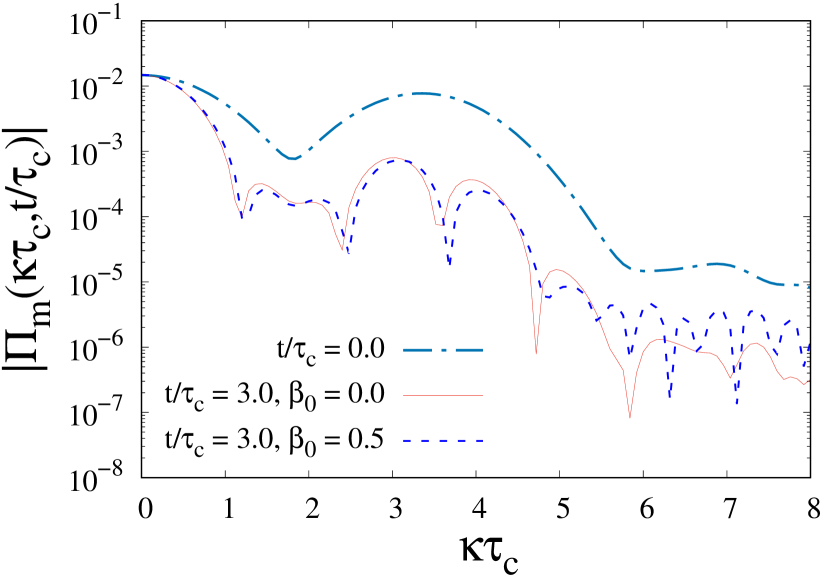
Figure 10: Momentum spectrum of energy density fluctuations at initial time (dash-dotted line), and at time $t/\tau_{c}=3.0$ in the absence (solid line) and in the presence (dashed line) of magnetic field for $\delta T_{1}=\delta T$.

We present in Fig. 10 the momentum spectrum [the modulus of Fourier modes, $|\Pi_{m}(\kappa^{\prime},t^{\prime})|$, versus $\kappa\tau_{c}$] of the energy density fluctuations of Fig. 9(b). In presence of magnetic field (dashed line), the high momentum dominant modes (at $\kappa\tau_{c}\approx$ 3.0 and 4.0) are more suppressed, while the low momentum modes ($\kappa\tau_{c}<1.2$) are somewhat less dissipated [as compared to $B=0$ (solid line)] at later time $t/\tau_{c}=3.0$. All these lead to qualitatively different characteristics of the fluctuations in the presence of magnetic field.

V. Phenomenological Implications

We shall discuss the phenomenological implications of the present study on certain important features and its related observables pertaining to relativistic heavy and light ion collisions, although it is potentially applicable to any small system whose constituents are electrically charged. For Au+Au collisions at c.m. energy $\sqrt{s_{NN}}=200$ GeV and impact parameter $b=8.0$ fm, the magnetic field can be as large as $|qB|\simeq 0.1m_{\pi}^{2}$ BMEq at a proper time $\tau\sim 0.2$ fm/c which is the timescale for saturated gluonic configuration to decay into (anti-)quarks and gluons shuryak0 ; BMEq . In the gluon saturation model, thermalization or hydrodynamization occurs at $\tau_{\rm eq}\simeq 0.4$ fm hydroSim when the magnetic field can still survive with appreciable strength; the magnetic field may persist in the entire partonic and possibly hadronic phase if the medium has a large electrical conductivity Hattori:2016lqx .

In the pre-equilibration dynamics at $\tau\lesssim 0.4$ fm, various short wavelength modes are present in the system with decay timescales smaller or comparable to this time (see Fig. 2 in Ref. Schenke12 ). Such fluctuation modes have sources from initial-state fluctuations in nucleon position, parton production and dynamics, hadron production and evolution. The magnetic field can increase the damping coefficient of mode oscillations and modify the characteristics of short wavelength fluctuations in the reaction plane (transverse to $B$) as demonstrated in this work. Consequently, this can have measurable effects on the azimuthal anisotropy of particle production/emission, namely the collective flow harmonics $v_{n}(p_{T})=\langle\cos n(\phi-\Psi_{n})\rangle$ (especially the odd harmonics that are driven by initial-state fluctuations) and the flow fluctuations Bhalerao:2014xra ; Giacalone:2017uqx ; saumia1 ; Schenke12i ; saumia2 ; ourRev ; ehr . In particular, the flow and flow-fluctuation observables would exhibit a noticeable suppression, reflecting the enhanced damping of fluctuation modes over the evolution time as found here (Fig. 6). Moreover, a smoother energy density profile, induced by suppression of short wavelength fluctuations in presence of magnetic field, should also show some qualitative changes in the power spectrum of flow fluctuations [$v_{n}(p_{T})$ versus $n$] at higher $n$.

The hydrodynamic fluctuations kapusta1 ; spal1 ; Chattopadhyay:2018dth and disturbances in the medium due to energy deposition by a partonic jet Casalderrey-Solana:2016jvj ; Tachibana:2017syd ; Milhano:2017nzm can prevail during the entire evolution of the system. The thermal or hydrodynamic fluctuations are correlated over short length scales that generate short-range correlation peak at small rapidity separation $\Delta y=y_{1}-y_{2}$ and nontrivial structure at large $\Delta y$ in the two-particle rapidity correlation kapusta1 ; spal1 ; Chattopadhyay:2018dth . Such long-range rapidity structures have been observed in multiparticle correlation measurements involving heavy ion and high-multiplicity light particle collision experiments at relativistic energies. Our analysis suggests magnetic damping of the peak at $\Delta y\approx 0$ and farther spread of the correlations in the rapidity separation. The disturbance generated by energy-momentum deposited in the vicinity of traversing hard jets in QGP and modifications of the jet shape and jet substructure observables due to (enhanced) rescattering of the emitted soft gluons in the medium will be sensitive to the magnetic field.

On the other hand, near the critical end point in the QCD phase diagram, the correlations among fluctuations diverge resulting in new fluctuation modes Stephanov:2010zz ; An:2019csj . The non-monotonous behavior in the event-by-event fluctuations with varying c.m. energy $\sqrt{s_{NN}}$ signals the location of the critical point. As the QCD critical point is expected to be at finite baryon density and at moderate collision energy Pandav:2022xxx , the strength of magnetic field will be relatively smaller, which however, decays slowly and can slow down some of the modes of critical fluctuations via increasing the damping coefficient. This can essentially enhance the magnitude of the observable signatures of the critical point. A detailed numerical simulation involving all the discussed features can provide quantitative effects of the magnetic field.

VI. Summary and Conclusions

In this paper we have studied the effects of magnetic field on the evolution of energy density fluctuations in the transverse direction. We find characteristic changes in the fluctuations at the timescale required by the system to achieve local thermal equilibrium. The magnetic damping of the underlying medium slows down the dissipation of the initial strength of the fluctuation near its peak while spreading out the fluctuation spatially to larger distances at early times. Increased Lorentz force at later times enforces larger damping of the fluctuation compared to the field-free case. A detailed Fourier mode analysis of the energy density fluctuations reveals that the low momentum modes, which survive longer in the entire evolution of the system, are strongly damped as compared to the fast evolving high momentum modes. The behavior is found to progressively increase with the strength of the magnetic field. However, at any instant of time, the magnetic field affects quantitatively more the high momentum modes as compared to the low momentum modes. This leads to a growth in the cutoff for the shortest wavelength fluctuations present in the system. If this cutoff is identified with the coarse-grained length scale in the hydrodynamic description of the medium, which then indicates an enhanced smoothening of energy density profile in presence of magnetic field. Further, the fluctuations in the direction transverse to the magnetic field are essentially affected, and moreover, various components of the energy-momentum tensor in the transverse direction are found to be modified differently, namely, $\hat{T}^{0x}$ is suppressed, while the $z$-components $\hat{T}^{0z}$ and $\hat{T}^{xz}$ are generated for fluid evolving along $x$-direction. As a result, additional spatial and momentum anisotropies can be generated in the three dimensional physical space by the magnetic field.

The present study has crucial phenomenological implications in the context of understanding the properties of quark-gluon plasma formed in relativistic heavy-ion collisions, and in general for any small systems whose constituents are electrically charged. In particular, the magnetic field can have noticeable impact on the potentially important observables, as for example, the flow harmonics and flow fluctuations, the hydrodynamic fluctuations, the jet substructure, and the dynamics of correlations and fluctuations close to the QCD critical point.

In the study, we have worked in the relaxation time approximation where the nonlinear effects, which can arise due to proper collision integral, has been ignored. The non-linearity can affect the evolution of energy density fluctuations as well as the effects of magnetic field studied in this work. We defer its inclusion for future studies.

I acknowledgments

We would like to thank Rajeev Bhalerao and Sunil Jaiswal for useful discussions. The simulations were performed at the High Performance Computing cluster at TIFR, Mumbai. The authors acknowledge financial support by the Department of Atomic Energy (Government of India) under Project Identification No. RTI 4002.

References

- (1) J. Adams, U.H. Danielsson, D. Grasso, and H. Rubinstein, Phys. Lett. B 388, 253 (1996).
- (2) H. Sotani, Phys. Rev. D 79, 084037 (2009).
- (3) K. Kiuchi, K. Kyutoku, Y. Sekiguchi, M. Shibata, and T. Wada, Phys. Rev. D 90, 041502(R) (2014).
- (4) K. Kiuchi, P. Cerdá-Durán, K. Kyutoku, Y. Sekiguchi, and M. Shibata, Phys. Rev. D 92, 124034 (2015).
- (5) K. Dionysopoulou, D. Alic, and L. Rezzolla, Phys. Rev. D 92, 084064 (2015).
- (6) A. Harutyunyan, A. Nathanail, L. Rezzolla, and A. Sedrakian, Eur. Phys. J. A 54, 191 (2018).
- (7) K. Kiuchi, K. Kyutoku, Y. Sekiguchi, and M. Shibata, Phys. Rev. D 97, 124039 (2018).
- (8) M. Anderson et al., Phys. Rev. Lett. 100, 191101 (2008).
- (9) T. Kawamura et al., Phys. Rev. D 94, 064012 (2016).
- (10) A. Endrizzi, R. Ciolfi, B. Giacomazzo, W. Kastaun, and T. Kawamura, Class. Quantum Grav. 33, 164001 (2016).
- (11) R. Ciolfi, Gen. Relativ. Gravit. 52, 59 (2020).
- (12) D.E. Kharzeev, L.D. McLerran, and H.J. Warringa, Nucl. Phys. A 803, 227 (2008).
- (13) B. Mller and A. Schfer, Phys. Rev. D 98, 071902(R) (2018).
- (14) K. Tuchin, J. Phys. G: Nucl. Part. Phys. 39, 025010 (2012).
- (15) U. Grsoy, D. Kharzeev, and K. Rajagopal, Phys. Rev. C 89, 054905 (2014).
- (16) R.K. Mohapatra, P.S. Saumia, and A.M. Srivastava, Mod. Phys. Lett. A 26, 2477 (2011).
- (17) A. Das, S.S. Dave, P.S. Saumia, and A.M. Srivastava, Phys. Rev. C 96, 034902 (2017).
- (18) S.S. Dave, P.S. Saumia, and A.M. Srivastava, Eur. Phys. J. Spec. Top. 230, 673 (2021).
- (19) G. Inghirami et al., Eur. Phys. J. C 76, 659 (2016).
- (20) G. Inghirami et al., Eur. Phys. J. C 80, 293 (2020).
- (21) L.D. Landau and E.M. Lifshitz, Electrodynamics of Continuous Media, Vol.8, Second Edition (Pergamon Press Ltd., 1984).
- (22) T. Kobayashi, J. Cosmol. Astropart. Phys. 05 (2014) 040.
- (23) A. Talebian, A. Nassiri-Rad, and H. Firouzjahi, Phys. Rev. D 105, 103516 (2022).
- (24) S. Schlichting and D. Teaney, Annu. Rev. Nucl. Part. Sci. 69, 447 (2019).
- (25) J. Berges, M.P. Heller, A. Mazeliauskas, and R. Venugopalan, Rev. Mod. Phys. 93, 035003 (2021).
- (26) H. Elfner and B. Müller, arXiv:2210.12056 [nucl-th].
- (27) K. Tuchin, Phys. Rev. C 88, 024911 (2013).
- (28) E. Stewart and K. Tuchin, Phys. Rev. C 97, 044906 (2018).
- (29) J.-J. Zhang et al., Phys. Rev. Research 4, 033138 (2022).
- (30) B. Schenke, S. Jeon, and C. Gale, Phys. Rev. Lett. 106, 042301 (2011).
- (31) B. Schenke, P. Tribedy, and R. Venugopalan, Phys. Rev. Lett. 108, 252301 (2012).
- (32) J.I. Kapusta, B. Müller, and M. Stephanov, Phys. Rev. C 85, 054906 (2012).
- (33) C. Chattopadhyay, R.S. Bhalerao, and S. Pal, Phys. Rev. C 97, 054902 (2018).
- (34) X. An, G. Başar, M. Stephanov, and H.-U. Yee, Phys. Rev. C 100, 024910 (2019).
- (35) M. Stephanov and Y. Yin, Phys. Rev. D 98, 036006 (2018).
- (36) A.P. Mishra, R.K. Mohapatra, P.S. Saumia, and A.M. Srivastava, Phys. Rev. C 77, 064902 (2008); Phys. Rev. C 81, 034903 (2010).
- (37) B. Schenke, S. Jeon, and C. Gale, Phys. Rev. C 85, 024901 (2012).
- (38) P.S. Saumia and A.M. Srivastava, Mod. Phys. Lett. A 31, 1650197 (2016).
- (39) W. Ke and Y. Yin, arXiv:2208.01046 [nucl-th].
- (40) G.S. Denicol, X.-G. Huang, E. Molnár, G.M. Monteiro, H. Niemi, J. Noronha, D.H. Rischke, and Q. Wang, Phys. Rev. D 98, 076009 (2018).
- (41) G.S. Denicol, E. Molnár, H. Niemi, and D.H. Rischke, Phys. Rev. D 99, 056017 (2019).
- (42) A.K. Panda, A. Dash, R. Biswas, and V. Roy, J. High Energy Phys. 03 (2021) 216; Phys. Rev. D 104, 054004 (2021).
- (43) P.L. Bhatnagar, E.P. Gross, and M. Krook, Phys. Rev. 94, 511 (1954).
- (44) J.L. Anderson and H.R. Witting, Physica 74, 466 (1974).
- (45) P. Romatschke, Eur. Phys. J. C 76, 352 (2016).
- (46) D. Bazow, M. Martinez, and U. Heinz, Phys. Rev. D 93, 034002 (2016).
- (47) M.P. Heller, A. Kurkela, M. Spaliński, and V. Svensson, Phys. Rev. D 97, 091503(R) (2018).
- (48) J. Brewer and P. Romatschke, Phys. Rev. Lett. 115, 190404 (2015).
- (49) P. Romatschke, Eur. Phys. J. C 77, 21 (2017).
- (50) A. Kurkela, U.A. Wiedemann, Eur. Phys. J. C 79, 776 (2019).
- (51) S.R. de Groot, W.A. van Leeuwen, Ch.G. van Weert, Relativistic Kinetic Theory: Principles and Applications, (North-Holland Publishing Company, Amsterdam, 1980).
- (52) M. Greif, C. Greiner, and Z. Xu, Phys. Rev. C 96, 014903 (2017).
- (53) Z. Chen, C. Greiner, A. Huang, and Z. Xu, Phys. Rev. D 101, 056020 (2020).
- (54) M. Kurian and V. Chandra, Phys. Rev. D 97, 116008 (2018).
- (55) D. Dash, S. Bhadury, S. Jaiswal, and A. Jaiswal, Phys. Lett. B 831, 137202 (2022).
- (56) L.D. Landau and E.M. Lifshitz, Course of Theoretical Physics, Vol.10: Physical Kinetics (Pergamon Press Ltd., Great Britain, 1981).
- (57) S. Jaiswal, C. Chattopadhyay, L. Du, U. Heinz, and S. Pal, Phys. Rev. C 105, 024911 (2022).
- (58) C. Chattopadhyay, U. Heinz, and T. Schfer, Phys. Rev. C 107, 044905 (2023).
- (59) C. Manuel and S. Mrówczyński, Phys. Rev. D 70, 094019 (2004).
- (60) B. Schenke, M. Strickland, C. Greiner, and M.H. Thoma, Phys. Rev. D 73, 125004 (2006).
- (61) M. Formanek, C. Grayson, J. Rafelski, and B. Mller, Annals Phys. 434, 168605 (2021).
- (62) C. Grayson, M. Formanek, J. Rafelski, and B. Mller, Phys. Rev. D 106, 014011 (2022).
- (63) P. Singha, S. Bhadury, A. Mukherjee, and A. Jaiswal, arXiv:2301.00544 [nucl-th].
- (64) G.S. Rocha, G.S. Denicol, and J. Noronha, Phys. Rev. Lett. 127, 042301 (2021).
- (65) N. Borghini, M. Borrell, N. Feld, H. Roch, S. Schlichting, and C. Werthmann, Phys. Rev. C 107, 034905 (2023).
- (66) W.H. Press, S.A. Teukolsky, W.T. Vetterling, and B.P. Flannery, Numerical Recipes in Fortran 77; The Art of Scientific Computing, 2nd ed. Vol. 1 (Syndicate, New York and Melbourne, 1997).
- (67) M. Prakash, M. Prakash, R. Venugopalan, and G. Welke, Phys. Rep. 227, 321 (1993).
- (68) P. Kalikotay, S. Ghosh, N. Chaudhuri, P. Roy, and S. Sarkar, Phys. Rev. D 102, 076007 (2020).
- (69) J. Adam et al. (STAR Collaboration), Phys. Rev. C 98, 014910 (2018).
- (70) L. Adamczyk et al. (STAR Collaboration), Nature (London) 548, 62 (2017).
- (71) L.P. Csernai, J.I. Kapusta, and T. Welle, Phys. Rev. C 99, 021901(R) (2019).
- (72) C. Loizides, J. Kamin and D. d’Enterria, Phys. Rev. C 97, 054910 (2018) [erratum: Phys. Rev. C 99, 019901 (2019)].
- (73) L. McLerran and R. Venugopalan, Phys. Rev. D 49, 2233 (1994); Phys. Rev. D 49, 3352 (1994).
- (74) E. Shuryak, Phys. Rev. C 80, 054908 (2009).
- (75) K. Hattori, S. Li, D. Satow, and H.U. Yee, Phys. Rev. D 95, 076008 (2017).
- (76) R.S. Bhalerao, J.Y. Ollitrault, and S. Pal, Phys. Lett. B 742, 94 (2015).
- (77) G. Giacalone, J. Noronha-Hostler, and J.Y. Ollitrault, Phys. Rev. C 95, 054910 (2017).
- (78) C. Chattopadhyay and S. Pal, Phys. Rev. C 98, 034911 (2018).
- (79) J. Casalderrey-Solana, D. Gulhan, G. Milhano, D. Pablos, and K. Rajagopal, J. High Energy Phys. 03 (2017) 135.
- (80) Y. Tachibana, N.B. Chang, and G.Y. Qin, Phys. Rev. C 95, 044909 (2017).
- (81) G. Milhano, U.A. Wiedemann, and K.C. Zapp, Phys. Lett. B 779, 409 (2018).
- (82) M.A. Stephanov, Prog. Theor. Phys. Suppl. 186, 434 (2010).
- (83) X. An, G. Başar, M. Stephanov, and H.U. Yee, Phys. Rev. C 102, 034901 (2020).
- (84) A. Pandav, D. Mallick, and B. Mohanty, Prog. Part. Nucl. Phys. 125, 103960 (2022).