Semantic Image Attack for Visual Model Diagnosis
Abstract
In practice, metric analysis on a specific train and test dataset does not guarantee reliable or fair ML models. This is partially due to the fact that obtaining a balanced, diverse, and perfectly labeled dataset is typically expensive, time-consuming, and error-prone. Rather than relying on a carefully designed test set to assess ML models’ failures, fairness, or robustness, this paper proposes Semantic Image Attack (SIA), a method based on the adversarial attack that provides semantic adversarial images to allow model diagnosis, interpretability, and robustness. Traditional adversarial training is a popular methodology for robustifying ML models against attacks. However, existing adversarial methods do not combine the two aspects that enable the interpretation and analysis of the model’s flaws: semantic traceability and perceptual quality. SIA combines the two features via iterative gradient ascent on a predefined semantic attribute space and the image space. We illustrate the validity of our approach in three scenarios for keypoint detection and classification. (1) Model diagnosis: SIA generates a histogram of attributes that highlights the semantic vulnerability of the ML model (i.e., attributes that make the model fail). (2) Stronger attacks: SIA generates adversarial examples with visually interpretable attributes that lead to higher attack success rates than baseline methods. The adversarial training on SIA improves the transferable robustness across different gradient-based attacks. (3) Robustness to imbalanced datasets: we use SIA to augment the underrepresented classes, which outperforms strong augmentation and re-balancing baselines. 111This paper was first submitted to NeurIPS on May 9, 2022.
1 Introduction
In Machine Learning (ML), error analysis of train and test data is a critical stage in model assessment and debugging. However, the conclusions extracted from the metric analysis on the train or test data do not guarantee reliability nor fairness, partially due to the fact that datasets are imperfect [20, 18]. Even with careful collection and filtering, data naturally contain biases. Furthermore, in the case of computer vision learning systems, having a uniform distribution over all conceivable variability of an object in an image (e.g., position, lighting, background) is typically impractical (i.e., exponential) and labels are prone to errors. The issue only grows more severe with large-scale datasets. ML models trained on these datasets inevitably inherit these imbalances and biases. These limitations also apply to test sets that are typically used for model evaluation. Such a vulnerability is a landmine that must be recognized and processed in order for ML applications to succeed. The question we strive to address in this study is whether there are alternative/better methods for discovering biases and performing model diagnostics in computer vision models instead of only relying on a test set.
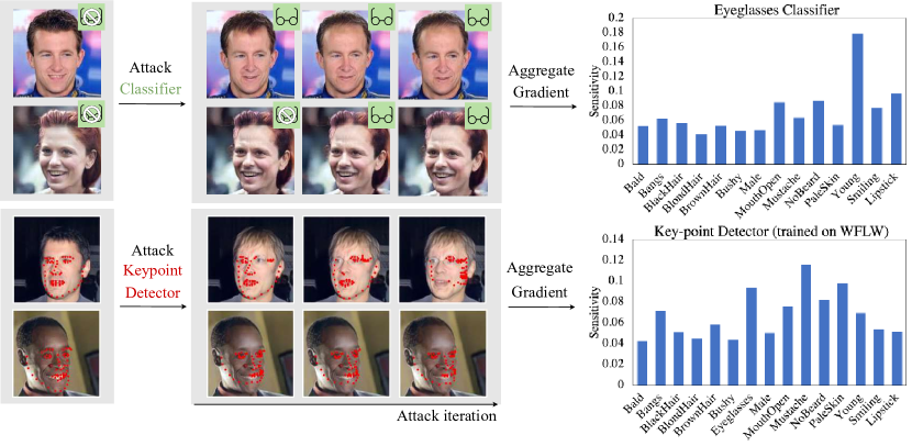
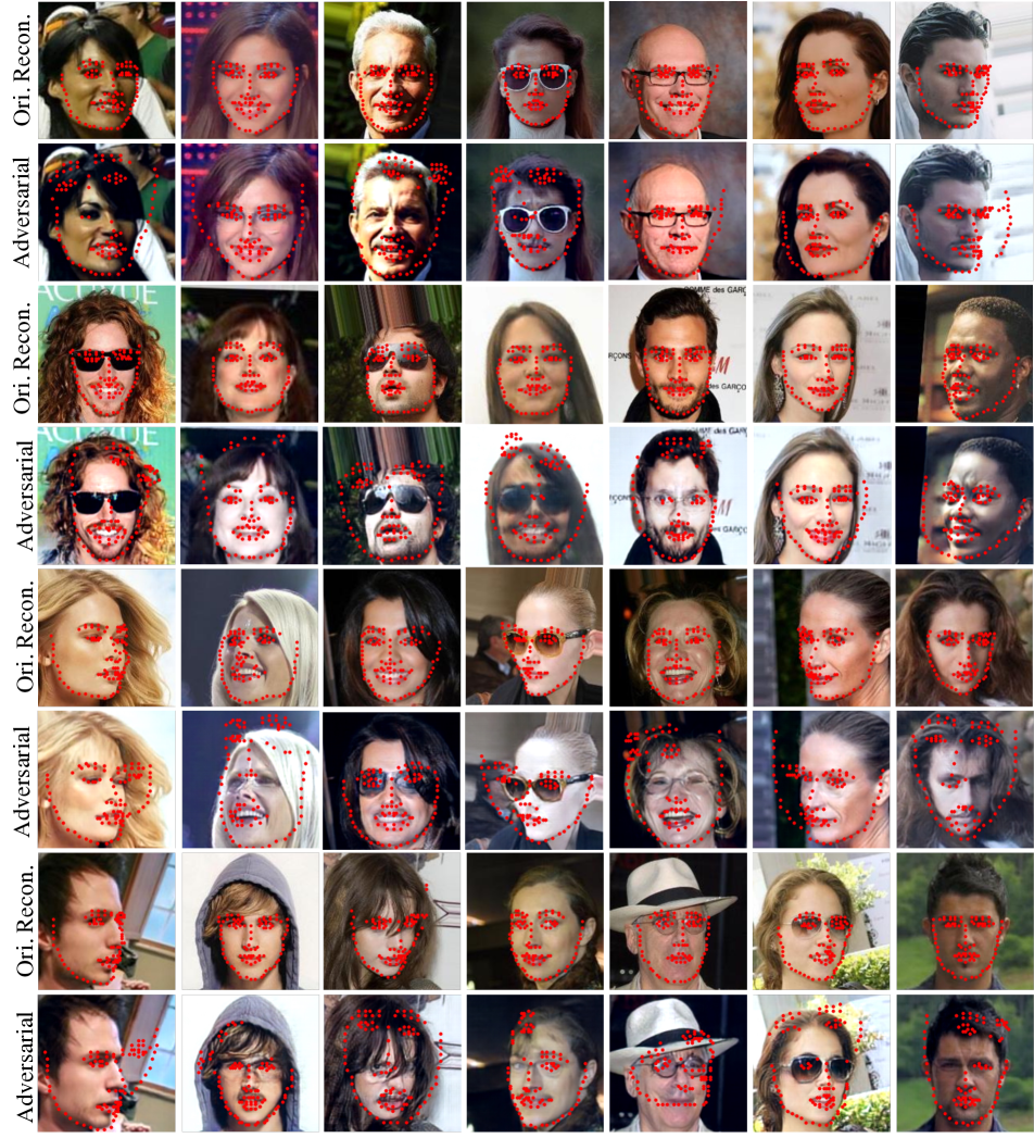
Fig. 1 illustrates the problems that this paper tries to address. Given an eyeglasses classifier (top two rows) or a keypoint detector (bottom two rows), which kind of face images will lead to misclassification or misdetection? How can we automatically discover these failure cases and robustify the model? How can we perform visual model diagnosis in a semantic attribute space? To accomplish these, we propose Semantic Image Attack (SIA), a new adversarial attack in a generative model of faces parameterized by attributes. In top left in Fig. 1, we see two images of faces without eyeglasses, and the model classifies them correctly. After several iterations of SIA (right column), our model is able to modify facial attributes (e.g., smile, eye color, facial hair) to mislead the eyeglass classifier. Also, our model builds a histogram of the sensitivity across attributes (i.e., visual model diagnosis). While evaluating the model resilience on a single attribute can be relatively straightforward, evaluating the model robustness for combinations of attributes can be quite challenging (due to the exponential nature of attribute combinations). SIA is able to jointly search over the space of attributes, and hence performs a multi-attribute attack for model diagnosis. Similarly, in Fig. 1, the bottom two rows illustrate the model diagnosis results for keypoint detection.
In addition to model diagnosis, SIA is able to robustify the target model by re-training the model on adversarial examples (see Fig. 1 middle columns). In our experiments, we also show the robustness from SIA is more transferable to other types of attacks than other competing attack methods. Finally, we show that SIA outperforms popular image augmentation techniques [4, 27] and re-balancing baselines when learning from imbalanced datasets.
2 Related Work
2.1 Adversarial Attacks
Gradient-guided image space perturbation attacks have been popular in robustifying ML models [8, 16]. The image perturbations generated by such attacks are small image changes typically imperceptible to humans. [29, 26] adopted such attacks on keypoint detectors to robustify detectors against adversarial perturbations. [25] was pioneering in using Generative Adversarial Networks (GANs) [7] to generate adversarial attacks. However, [25] only allowed a limited perturbation bound and required individually trained GANs for every target ML model. A major issue of previous methods is the lack of interpretability of the attack. To address this issue, [17] used the interpolation of semantic feature maps to generate attacks, and showed the effectiveness in terms of the attack’s success rate in classification and detection problems. [6] also modeled the perturbations in the attribute space, and showed that the attribute space can improve model robustness. However, this work aims to find perturbations in samples that do not change labels, and their model is not robust to small perturbation attacks in the image space. Moreover, [6] did not provide interpretability into the failures of the computer vision model. Similarly, [14] sampled images in the latent space of a GAN to generate strong attacks, but their attacks are not interpretable in the attribute space. [11] conducted model attacks only in the attribute space using the attribute-assisted GAN (AttGAN) [10]. This approach does not attack the image space and does not constrain the scale of parametric gradients, which leads to generating unrealistic images.
Unlike previous work in the adversarial attack literature, SIA performs gradient-guided attack simultaneously in the image and a pre-defined attribute space. As we will show in the experimental section, performing gradient ascent only in the attribute space leads to unstable results. In addition, our approach only uses one GAN backbone [10] to attack all target models (i.e., AttGAN can be used to evaluate any computer vision model). Finally, our method provides a histogram of the sensitivity of the target models across attributes of interest. This information can be critical to gather insights into the fairness and robustness of the model.
2.2 Bias and Fairness Analysis
[2, 5] showed that by traversing images in the GAN latent space, one can visualize the attribute-wise sensitivity of a target classifier. But such a process requires manual annotation of the generated images, which is expensive and infeasible for large attribute spaces. Recently, [13] used StyleGAN [12] to learn a target-model-dependent style/attribute space, which allows a human to interpret the target models’ behavior in terms of attributes. Furthermore, several previous works proposed fairness metrics to evaluate a model without a fair test set [9, 18, 28]. While previous fairness metrics focus on a model’s statistical behavior across attributes, SIA focuses on the model’s decision for each instance (though individual sensitivities can be further aggregated to get sub-population sensitivity, see Fig. 1). Moreover, SIA is able to search over attribute combinations.
3 Semantic Image Attack (SIA)
This section describes our SIA algorithm starting with the notation.
Target model (): Let , parameterized by , be the target model that we want to improve or perform model diagnosis on. In this paper, we cover two types of neural network models : an attribute classifier and a keypoint detector.
An attribute classifier takes an image as input and outputs , the conditional probability of attribute given , where is the attribute space. Without loss of generality, we consider binary classifiers. Given the ground truth class label of the image , the classification loss is defined as the binary cross-entropy .
The keypoint detector takes an image as input and outputs , the probability heatmap of the keypoints , where is the 2D pixel coordinate space. Given a training image with ground truth facial keypoints , the loss is defined as the mean squared error between the predicted heatmap and the ground-truth heatmap corresponding to , see [21] for details.
Adversary (): For each input image , an adversarial example is a synthesized image that misleads the target model to produce outputs that are far away from the ground truth or changes the label of the classifier. Different from traditional adversarial attack methods, SIA generates adversarial examples under a combination of perturbations in the attribute and image spaces.
SIA consists of two main components: (1) an AttGAN , , , where the encoder maps an input image to a latent vector, the decoder takes as an input the concatenation of and the attribute vector to generate an image; (2) a pretrained target model to be diagnosed.
3.1 Generating Iterative Adversaries
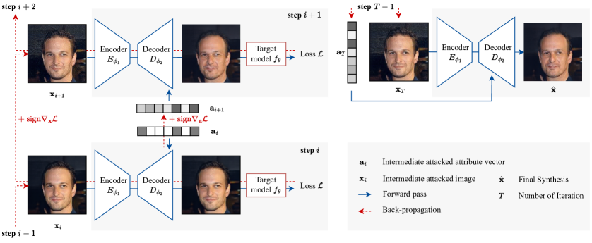
Our framework uses both the attribute space and the image space to iteratively generate adversarial images . We iteratively compute gradient ascent in the attribute space and the image space. An advantage of optimizing over the attribute and image space is an improved adversarial space, that leads to a better generation of adversarial examples (see experiment section).
The procedure to jointly update the attribute vectors and images is as follows:
| (1) | ||||
The adversarial example is an image space projection of a fine-grained perturbation of the original input image at both pixel and attribute levels. During the process, our SIA framework manipulates the attribute vector in a predefined attribute space such that the target model is compromised. Note that each iteration of the updates will be clipped with a radius to make sure that the perturbation is bounded and valid. The pixel-level perturbed image is fed into to encode the adversarial information into the latent vector, which is concatenated with the perturbed attribute vector. Specifically, instead of directly perturbing the output image, which may significantly harm the perceptual quality, we perturb the input attribute and the image and let project the perturbed image and attribute back to the image manifold. To prevent synthesis collapse, we adopt the projection onto the ball of radius to constrain the optimization. The projection to generate the final adversarial example is formulated as . An overview of our SIA framework is shown in Figure 2.
At this point, it is important to notice that perturbing in both the image space and attribute space produces higher attack success rate and finer visual adversarial images. Also, we do it for a fair comparison with traditional methods. Recall that directly perturbing the semantic space limits the attacking capability. Our hybrid attack gives us the flexibility to analyze both the semantic and pixel-level robustness of the model. In fact, SIA’s pixel-level perturbation helps to avoid exaggerated semantic variation that makes the image generation collapse. An ablation study that illustrates the advantages of perturbing in both the image and attribute space is included in the experimental section.
3.2 Interpreting and Improving the Target Model
Given a set of image-attribute pairs (), we run iterations of Eq. 1 and store all the generated adversaries. By calculating the absolute variation of attributes during the generation of adversaries , we can discover the most sensitive attribute(s) to the target model in the ’s attribute space. We define the sensitivity vector containing sensitivities (in the range of ) of the target model on each attribute as follows:
| (2) |
Each value in will represent the average perturbation of the corresponding attribute across all sampled images. Note that this method can be extended to select top-k attributes that have a greater influence on the prediction of the target model. The generated adversaries are associated with more diverse attribute vectors , which can be considered as an augmented dataset for adversarial training. See Algorithm 1 for more details on how to generate adversaries and sensitivity analysis.
4 Experiments
This section explains the experimental validation to demonstrate the benefits of SIA for visual model diagnostics, improved robustness against visual attacks, and imbalanced robustness.
4.1 Experimental Setups
Attribute-assisted GAN: Our backbone of AttGAN is trained on the whole CelebA dataset [15], using attributes222we used Bald, Bangs, Black_Hair, Blond_Hair, Brown_Hair, Bushy_Eyebrows, Eyeglasses, Male, Mouth_Slightly_Open, Mustache, No_Beard, Pale_Skin, Young, Smiling, Wearing_Lipstick. Images are center cropped, resized to , and normalized using the ImageNet normalization. ’s encoding and decoding dimensions are both 64. Shortcuts and inject layers are activated, and the Wasserstein loss [1] is used. We used the codes provided by [10]333https://github.com/elvisyjlin/AttGAN-PyTorch.
Attribute Classifier: Our classifiers are fine-tuned from TorchVision’s pre-trained ResNet50. Unless otherwise stated, we trained binary classifiers on the CelebA training set [15]. For training, we used the Adam optimizer with a learning rate of 0.001 and batch size of 128. The seed for random number generation is 42 for Numpy and PyTorch.
Keypoint Detector: We used the HR-Net architecture [21]. We trained two models, one trained on the Wilder Facial Landmark in the Wild (WFLW) dataset [24] and the other on the Microsoft (Fake-it) synthetic dataset [23]. To train the two keypoint detectors, we used all images () from the WFLW dataset and the first images from the Fake-it dataset, respectively. We trained with keypoints on the WFLW dataset and keypoints on the Fake-it dataset.


4.2 Visual Model Diagnosis
After training a deep learning model and tuning hyper-parameters of the model on a validation set, an important step is error analysis. The error analysis includes analyzing where the model fails on test data and making systematic changes based on the insights. However, in some scenarios, it is difficult to collect test data across all possible attributes of interest in a uniform manner. Instead of collecting test data, this section describes how SIA can be used for model diagnosis and provides insights into the image attributes that make the model fail.
4.2.1 Diagnosis visualization
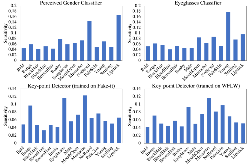
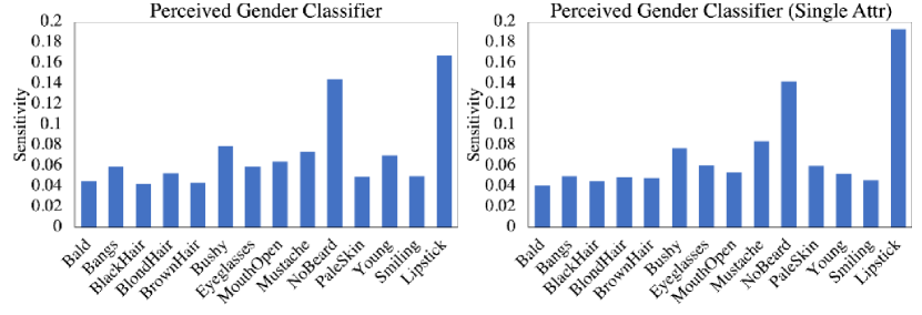
We trained binary classifiers on the following attributes from CelebA: Attractive, Arched_Eyebrows, Blurry, Chubby, Eyeglasses, Male, No_Beard, Sideburns with the setup mentioned in Section 4.1. In addition, we trained two keypoint detection algorithms, one on real images and another one on synthetic images, using the same architecture HR-Net [21]. SIA reports the sensitivity of the target model w.r.t. different attributes, which is formalized in Eq. 2. We selected the first images in CelebA to evaluate the sensitivities. Fig. 3 illustrates the histogram for the classifier (first row) and keypoint detector (second row) towards different attributes, according to Eq. 2. For clearer visualization, we have normalized the sensitivity for each attribute by the sum of sensitivities. We can see that for the perceived-gender classifier, lipstick and beard are the most sensitive attributes. Similarly, we discovered that changing specific attributes can largely affect the outcome of a well-trained keypoint detection model. Interestingly, both keypoint detectors are very sensitive to mustache and eyeglasses, and not very sensitive to hair color or perceived gender. This is expected, since keypoints have a higher density around the eyes and mouth region, and modification of these regions can be critical to the accuracy.
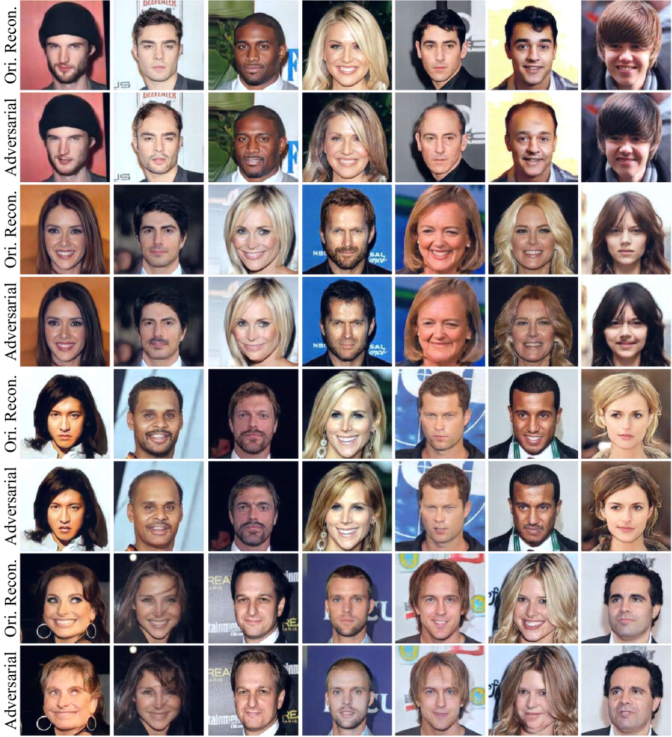
Fig. 4 shows example images of SIA attacking the two target models. For the perceived-gender classifier in Fig. 4 (a), we can see from the first four columns that mutating the lipstick and beard attributes will influence the model’s prediction. The last three columns show that mutating other attributes including hair color, skin color, and bangs can also affect the model decision. Fig. 4 (b) shows that SIA changes attribute such as eyeglasses, pale skin, or mustache to cause keypoints misdetection in facial images. This sensitivity analysis and adversarial examples can provide insights into the kind of images where the keypoint detector or classifier fails, and generate adversaries to improve performance. More adversarial examples and histograms for the remaining attributes are shown in Appendix A and B.
| PSNR () | SSIM () | |||||||||||
| SPT-50 | SIA-50 (Attr) | SIA-50 (Full) | SPT-200 | SIA-200 (Attr) | SIA-200 (Full) | SPT-50 | SIA-50 (Attr) | SIA-50 (Full) | SPT-200 | SIA-200 (Attr) | SIA-200 (Full) | |
| 26.63 | 41.98 | 42.24 | 19.43 | 31.21 | 33.94 | 0.9083 | 0.9929 | 0.9930 | 0.7732 | 0.9602 | 0.9718 | |
| 14.18 | 22.36 | 28.25 | 13.59 | 20.16 | 25.75 | 0.6385 | 0.8573 | 0.9285 | 0.6230 | 0.8037 | 0.8926 | |
4.2.2 Image quality evaluation
We evaluated the image perceptual quality for adversarial examples generated by SPT [11] and SIA. To interpret Table 1, SPT-50 () stands for the adversarial examples generated by SPT with 200 iterations and step size of . The tables show that SIA’s image quality is better than SPT under both PSNR (Peak Signal to Noise Ratio) and SSIM (Structured Similarity Indexing Method) [22] metrics. We can see that perturbing in both image space and attribute space produces visually finer adversarial images. In fact, SIA’s pixel-level perturbation helps to avoid exaggerated semantic variation that makes the image generation collapse.
4.2.3 Sensitivity by single-attribute optimization
We can also perform SIA independently for every single attribute and organize the sensitivities as the histogram on the right in Fig. 6. We can see that SIA’s histograms, no matter multi-attribute or single-attribute, support consistent analysis of most sensitive attributes. However, it is worth noting that a greedy single attribute perturbation can be computationally expensive for a large attribute space (e.g., 15 attributes). It is very time-consuming to adversarially traverse a single attribute over the dataset and repeat 15 times (i.e., repeat for each attribute) in a grid-search manner. Jointly optimizing all attributes is more time-effective and comprehensive (i.e., exploring a continuous space across all attributes) as the histogram on the left.
4.3 Attack Effectiveness
This section compares SIA to popular gradient-based adversarial attacks in a white-box setting for the attribute classifiers. Then an ablation study is conducted to demonstrate the effectiveness of various components in SIA, including the use of attribute and image perturbations.
4.3.1 Attack success rate
SIA constrains the perturbation bounds of attribute space () and image space () separately. The attributes that do not overlap with the target model range between with a step size . The attribute that is equivalent to the target classifier is constrained to be a small constant depending on the attribute being classified. We iteratively perturbed the input image bounded by with . The number of steps for both the attribute space and image space will be . The evaluated subset in CelebA corresponds to the first images.
We used the FGSM [8] and PGD [16] under norm of different perturbation bounds as baseline methods. For PGD, the iteration step size with 200 steps in total. For FGSM, the attack will iterate once within a bounded perturbation. In the adversarial training experiment, we additionally compared with SPT [11] using the same attribute space as SIA. However, we did not compare with [14] since their method samples adversarial examples from StyleGAN, which does not support attacking existing images. We also did not compare with [13] because their method requires training a separate model on StyleGAN’s original training data for each target model.
Table 2 shows the attack success rates for different perturbation-based attacks on multiple target classifiers. Notably, we can see that SIA achieves performance comparable to traditional attacks with smaller perturbations.
| Classifier | FGSM | PGD | SIA | |
| 1.5/255 | Eyeglasses | 28.01 | 49.85 | 68.20 |
| Perceived Gender | 56.31 | 65.32 | 88.19 | |
| 2/255 | Eyeglasses | 42.83 | 87.79 | 94.82 |
| Perceived Gender | 75.27 | 87.19 | 92.44 | |
| 4/255 | Eyeglasses | 78.90 | 99.94 | 99.99 |
| Perceived Gender | 97.33 | 97.41 | 98.53 |
4.3.2 Ablation for image v.s. attribute space
This experiment analyzes the attack success rate when attacking the image and/or the attribute space (see Table 3). Original reconstruction refers to the images reconstructed by without any perturbations. I/A refers to only updating the image/attribute space during the attack. PI/PA refers to partially updating the image/attribute space in the first iterations of the total iterations. Note that the Attr-space setting is different from SPT [11] since SIA uses linearization to constrain the gradient updates to stabilize the attack. As expected, the attack effectiveness is much higher regardless of using attribute space alone or in combination.
| Eyeglasses | Goatee | Age | Sideburns | |
| OR | 0.02 | 3.49 | 0.15 | 3.32 |
| I | 1.83 | 13.58 | 6.10 | 12.51 |
| I + PA | 18.25 | 26.54 | 30.16 | 22.46 |
| A | 32.67 | 83.59 | 90.90 | 67.97 |
| A + PI | 44.26 | 79.82 | 85.98 | 70.65 |
| Full | 68.20 | 90.51 | 90.38 | 87.08 |
4.3.3 Extending attribute space
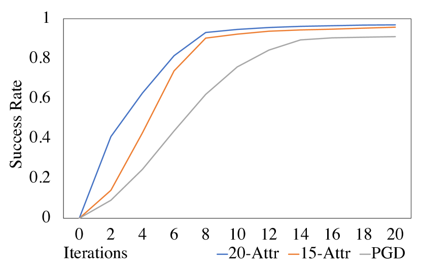
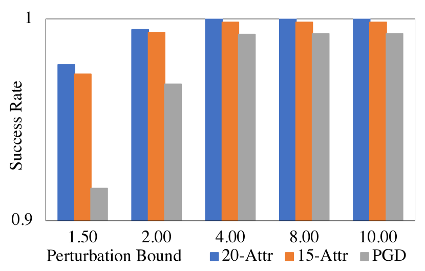
We experimented with an alternative attribute space of attributes for . We removed Black_Hair, Brown_Hair, Bushy_Eyebrows, Eyeglasses, Male(perceived), No_Beard, Young(perceived), Wearing_Lipstick which are either attribute of target classifier or attributes with overlapped concepts. Then we added Narrow_Eyes, Oval_Face, Pale_Skin, Pointy_Nose, Receding_Hairline, Rosy_Cheeks, Sideburns, Straight_Hair, Big_Lips, Big_Nose, Chubby, Goatee, Heavy_Makeup, High_Cheekbones. Compared with the attribute space used in our main experiment, this alternative attribute space covers more semantic variations in facial data. Fig. 7(a) shows the success rate for the attractive classifier. PGD refers to the implemented PGD attack [16]. The larger the attribute space, the higher the success rate, and the attack converges in fewer iterations. This is not surprising because the larger semantic space helps to search the combination of adversarial attributes more effectively. Fig. 7(b) shows that with the same perturbation bound setting, the extended will give a stronger attack on the target classifier.
4.4 Adversarial Training
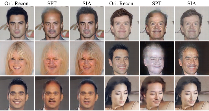
In this experiment, we evaluated the effectiveness of SIA to improve adversarial robustness. We adopted the setting such that the target model is fine-tuned with adversarial examples for one epoch. Table 4 shows how SIA can be used effectively for re-fitting adversarial examples generated by Algorithm 1. SIA-Adv, PGD-Adv, SPT-Adv are eyeglasses classifiers adversarially trained with adversarial examples generated by the corresponding attack method from the first images of CelebA. The perturbation bound is . Non-adversarial training means the regular classifier trained in Section 4.2. All models are evaluated on the first images from the CelebA test set that the models have never seen before. Results show that the robustness of SIA adversarial training is transferable to other attack methods, but not vice versa (i.e., see how the column SIA-Adv works well across all the attacks). This is because our adversarial example constructs both conceptual shifts in the semantic space and noise shift in the image space, which introduces richer information during the adversarial training compared to traditional perturbation attacks. Fig. 8 shows the visual comparison of SIA and SPT adversaries on the eyeglasses classifier. SPT generates less fine-controlled semantic changes because updating only the attribute space results in large changes across many attributes. More visual comparisons of different baselines for adversarial training are reported in Appendix C.
| Non-Adv | PGD-Adv [16] | SPT-Adv [11] | SIA-Adv | |
| Clean Test Set | 99.63 | 99.54 | 99.51 | 99.52 |
| FGSM () | 73.97 | 86.55 | 77.76 | 94.01 |
| PGD () | 50.63 | 81.98 | 16.52 | 86.90 |
| SIA () | 12.59 | 27.90 | 74.01 | 67.07 |
| FGSM () | 22.47 | 22.09 | 41.78 | 45.51 |
| SIA () | 4.56 | 10.85 | 10.55 | 12.57 |
4.4.1 Standard deviation of attribute robustness
We established a measure named Standard Deviation of Attribute Robustness (SDAR) to understand the final variance of our model across attributes. For a given classifier , SIA generates the sensitivity histogram based on the attribute perturbation vector of length . The SDAR metric is defined as the standard deviation of the sensitivity values .
Ideally, an unbiased model should have equal sensitivity across all attributes, hence a decrease in the standard deviation will indicate that the model is less biased. To validate the method, we calculated SDARs after evaluating different models from adversarial training. The test data was the first images of CelebA test set. We evaluated the SDAR metric under two bounds () of SIA. Table 5 shows the results. We can see that the non-adv classifiers will have larger and the adversarially-trained models have smaller since the model generalization is improved by the adversarial training process. By optimizing both the attribute and the image space, SIA-Adv better generalizes over attributes than regular classifiers.
| Non-Adv | PGD-Adv [16] | SPT-Adv [11] | SIA-Adv (Ours) | |
| 0.1145 | 0.0917 | 0.0852 | 0.0781 | |
| 0.1419 | 0.1270 | 0.1253 | 0.1056 |
4.5 Robustness to Imbalanced Datasets
This section reports experiments to evaluate the robustness of SIA in learning from imbalanced datasets. In these situations, it is vital to develop algorithms that are not biased toward the majority class. While data augmentation and re-weighting are commonly used techniques, we show how SIA provides an alternative that generates semantically meaningful augmentation with high visual quality.
We trained two attribute classifiers, for eyeglasses and bangs, using the ResNet50 architecture. We generated a synthetically unbalanced dataset to produce a controlled imbalanced environment. For training, we randomly sampled images from CelebA training set such that are positive and are negative. We trained the classifiers from random initialization. For testing, we use balanced test data including random positive-label images and negative-label images from CelebA test set.
Table 6 shows the precision, recall, and accuracy for several imbalanced learning strategies. We compared SIA to five data augmentation and re-balancing approaches. The Non-Adv attribute classifiers are trained on the synthetic data with 1:99 CelebA training set. The CutMix [27] baselines are augmented with action probability and learning rate . We followed PyTorch’s implementation on AutoAugment [4]. We also included two commonly used baselines to deal with imbalanced data: Reweighting and Resampling. Reweighting means upweighting the under-represented samples based on the proportion of class samples. Resampling means duplicating the under-represented samples until different classes have the same number of samples. SIA refers to classifiers augmented by randomly sampling our adversarial images. SIA + Reweight is the scheme where the reweighting is performed on our SIA-augmented dataset. Results show that SIA can effectively be used to augment imbalanced datasets, outperforming other widely used augmentation methods. One possible reason is that SIA generates semantically meaningful augmentations, different from CutMix and AutoAugment. Finally, we conduct a similar experiment with pre-trained classifiers in Appendix D. We show that the difference in accuracy between the methods narrows down considerably if we pre-train the classifiers. This is not surprising, since pre-training with sufficient data provides robust features that are less prone to imbalance.
| Strategy | Prec. | Recall | Acc. (%) | |
| Eyeglasses | Non-adv classifier | 0.9985 | 0.8052 | 90.20 |
| Reweighting | 0.9995 | 0.8368 | 91.82 | |
| Resample | 0.9984 | 0.7700 | 88.44 | |
| CutMix | 0.9963 | 0.3236 | 66.12 | |
| AutoAugment | 0.9975 | 0.8004 | 89.92 | |
| SIA-Adv (ours) | 0.9991 | 0.8864 | 94.28 | |
| SIA-Adv + Reweight (ours) | 0.9991 | 0.8856 | 94.24 | |
| Bangs | Non-adv classifier | 0.9847 | 0.2576 | 62.68 |
| Reweighting | 0.9912 | 0.2708 | 63.42 | |
| Resample | 0.9935 | 0.1840 | 59.14 | |
| CutMix | 1.0000 | 0.0000 | 50.00 | |
| AutoAugment | 0.9701 | 0.0260 | 51.26 | |
| SIA-Adv (ours) | 0.9791 | 0.4116 | 70.14 | |
| SIA-Adv + Reweight (ours) | 0.9854 | 0.5960 | 79.36 |
5 Conclusions and Future Work
This paper introduced SIA, an attribute-assisted adversarial method with applications in model diagnosis, improving target model robustness, and increasing the success of visual attacks. A major appeal of our technique is the capacity of analyzing a deep learning model without a carefully designed test set. SIA reveals the dependencies between attributes and model outputs, which helps interpret the biases learned by models during prediction. We hope our results pave the way for new tools to analyze models and inspire future work on mitigating such biases.
While we showed the benefits of our technique in two computer vision problems, our approach is applicable to any end-to-end differentiable target deep learning model. It is unclear how to extend this approach to non-differentiable ML models, and more research needs to be done. Our method works with white-box attacks since our primary motivation is to diagnose a known model. More research needs to be done to address black-box attacks. Furthermore, we have illustrated the power of SIA only in the context of faces, but our method can extend to generative models that have been trained with other attributes of interest and can be applied to other visual domains.
References
- [1] Martin Arjovsky, Soumith Chintala, and Léon Bottou. Wasserstein Generative Adversarial Networks. In ICML, 2017.
- [2] Guha Balakrishnan, Yuanjun Xiong, Wei Xia, and Pietro Perona. Towards Causal Benchmarking of Bias in Face Analysis Algorithms. In ECCV, 2020.
- [3] Nicholas Carlini and David Wagner. Towards Evaluating the Robustness of Neural Networks. In IEEE SP, 2017.
- [4] Ekin D. Cubuk, Barret Zoph, Dandelion Mane, Vijay Vasudevan, and Quoc V. Le. AutoAugment: Learning Augmentation Strategies From Data. In CVPR, 2019.
- [5] Emily L. Denton, Ben Hutchinson, Margaret Mitchell, Timnit Gebru, and Andrew Zaldivar. Image Counterfactual Sensitivity Analysis for Detecting Unintended Bias. In CVPR, 2019.
- [6] Tejas Gokhale, Rushil Anirudh, Bhavya Kailkhura, Jayaraman J. Thiagarajan, Chitta Baral, and Yezhou Yang. Attribute-Guided Adversarial Training for Robustness to Natural Perturbations. In AAAI, 2021.
- [7] Ian Goodfellow, Jean Pouget-Abadie, Mehdi Mirza, Bing Xu, David Warde-Farley, Sherjil Ozair, Aaron Courville, and Yoshua Bengio. Generative Adversarial Nets. In Z. Ghahramani, M. Welling, C. Cortes, N. Lawrence, and K.Q. Weinberger, editors, NeurIPS, 2014.
- [8] Ian J. Goodfellow, Jonathon Shlens, and Christian Szegedy. Explaining and Harnessing Adversarial Examples. In Yoshua Bengio and Yann LeCun, editors, ICLR, 2015.
- [9] Moritz Hardt, Eric Price, and Nathan Srebro. Equality of Opportunity in Supervised Learning. arXiv preprint arXiv:1610.02413, 2016.
- [10] Z. He, W. Zuo, M. Kan, S. Shan, and X. Chen. AttGAN: Facial Attribute Editing by Only Changing What You Want. In IEEE TIP, 2019.
- [11] Ameya Joshi, Amitangshu Mukherjee, Soumik Sarkar, and Chinmay Hegde. Semantic Adversarial Attacks: Parametric Transformations That Fool Deep Classifiers. In ICCV, 2019.
- [12] Tero Karras, Samuli Laine, and Timo Aila. A Style-Based Generator Architecture for Generative Adversarial Networks. In CVPR, 2019.
- [13] Oran Lang, Yossi Gandelsman, Michal Yarom, Yoav Wald, Gal Elidan, Avinatan Hassidim, William T. Freeman, Phillip Isola, Amir Globerson, Michal Irani, and Inbar Mosseri. Explaining in Style: Training a GAN To Explain a Classifier in StyleSpace. In ICCV, 2021.
- [14] Dongze Li, Wei Wang, Hongxing Fan, and Jing Dong. Exploring Adversarial Fake Images on Face Manifold. In CVPR, 2021.
- [15] Ziwei Liu, Ping Luo, Xiaogang Wang, and Xiaoou Tang. Deep Learning Face Attributes in the Wild. In ICCV, 2015.
- [16] Aleksander Madry, Aleksandar Makelov, Ludwig Schmidt, Dimitris Tsipras, and Adrian Vladu. Towards Deep Learning Models Resistant to Adversarial Attacks. In ICLR, 2018.
- [17] Haonan Qiu, Chaowei Xiao, Lei Yang, Xinchen Yan, Honglak Lee, and Bo Li. SemanticAdv: Generating Adversarial Examples via Attribute-conditioned Image Editing. In ECCV, 2020.
- [18] Vikram V. Ramaswamy, Sunnis S. Y. Kim, and Olga Russakovsky. Fair Attribute Classification through Latent Space De-biasing. In CVPR, 2021.
- [19] Olaf Ronneberger, Philipp Fischer, and Thomas Brox. U-Net: Convolutional Networks for Biomedical Image Segmentation. In MICCAI, 2015.
- [20] Prasanna Sattigeri, Samuel C. Hoffman, Vijil Chenthamarakshan, and Kush R. Varshney. Fairness GAN. arXiv preprint arXiv:1805.09910, 2018.
- [21] Jingdong Wang, Ke Sun, Tianheng Cheng, Borui Jiang, Chaorui Deng, Yang Zhao, Dong Liu, Yadong Mu, Mingkui Tan, Xinggang Wang, Wenyu Liu, and Bin Xiao. Deep High-Resolution Representation Learning for Visual Recognition. In IEEE TPAMI, 2019.
- [22] Zhou Wang, A.C. Bovik, H.R. Sheikh, and E.P. Simoncelli. Image Quality Assessment: from Error Visibility to Structural Similarity. In IEEE TIP, 2004.
- [23] Erroll Wood, Tadas Baltrušaitis, Charlie Hewitt, Sebastian Dziadzio, Matthew Johnson, Virginia Estellers, Thomas J. Cashman, and Jamie Shotton. Fake It Till You Make It: Face Analysis in the Wild Using Synthetic Data Alone. arXiv preprint arXiv:2109.15102, 2021.
- [24] Wayne Wu, Chen Qian, Shuo Yang, Quan Wang, Yici Cai, and Qiang Zhou. Look at Boundary: A Boundary-Aware Face Alignment Algorithm. In CVPR, 2018.
- [25] Chaowei Xiao, Bo Li, Jun yan Zhu, Warren He, Mingyan Liu, and Dawn Song. Generating Adversarial Examples with Adversarial Networks. In IJCAI, 2018.
- [26] Qingsong Yao, Zecheng He, Hu Han, and S. Kevin Zhou. Miss the Point: Targeted Adversarial Attack on Multiple Landmark Detection. In MICCAI, 2020.
- [27] Sangdoo Yun, Dongyoon Han, Sanghyuk Chun, Seong Joon Oh, Youngjoon Yoo, and Junsuk Choe. CutMix: Regularization Strategy to Train Strong Classifiers With Localizable Features. In ICCV, 2019.
- [28] Brian Hu Zhang, Blake Lemoine, and Margaret Mitchell. Mitigating Unwanted Biases with Adversarial Learning. In AAAI, 2018.
- [29] Congcong Zhu, Xiaoqiang Li, Jide Li, and Songmin Dai. Improving Robustness of Facial Landmark Detection by Defending Against Adversarial Attacks. In ICCV, 2021.
Supplementary Material
Appendix A SIA Adversarial Images
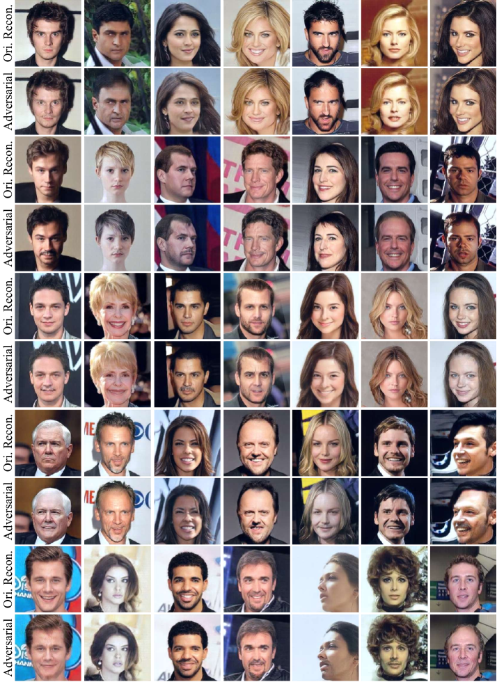
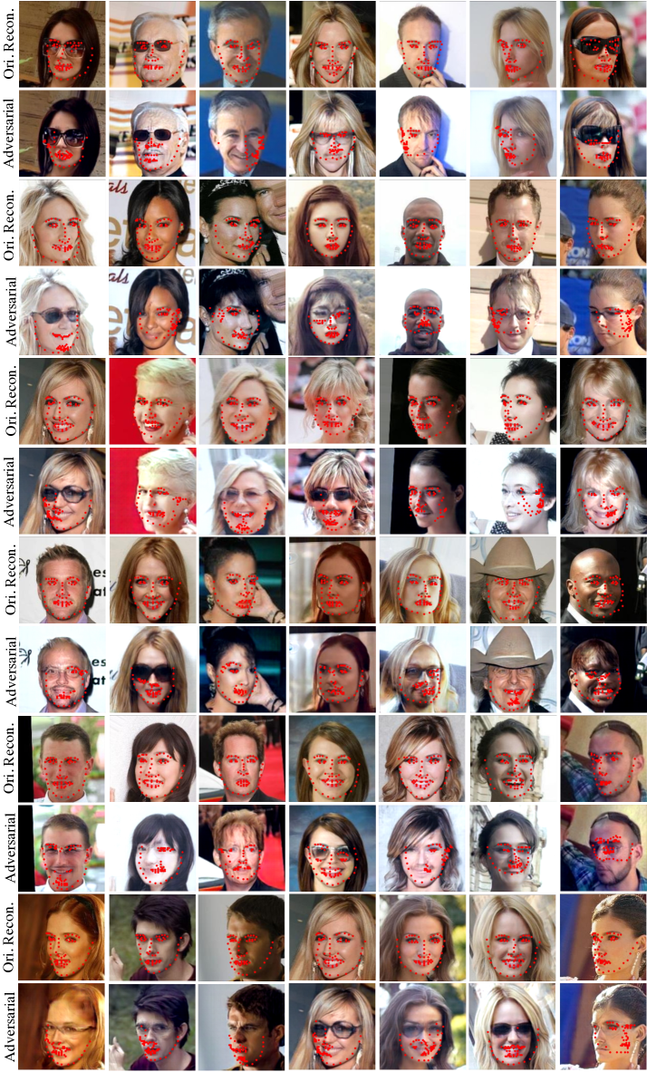
Fig. 9 and Fig. 10 show additional examples of adversarial images generated by SIA for different target models. We find the adversarial semantic shifts on keypoint detectors are visually greater than that on classifiers. These results show that detectors are more robust to semantic shifts than classifiers.
Appendix B Histograms for Model Interpretation
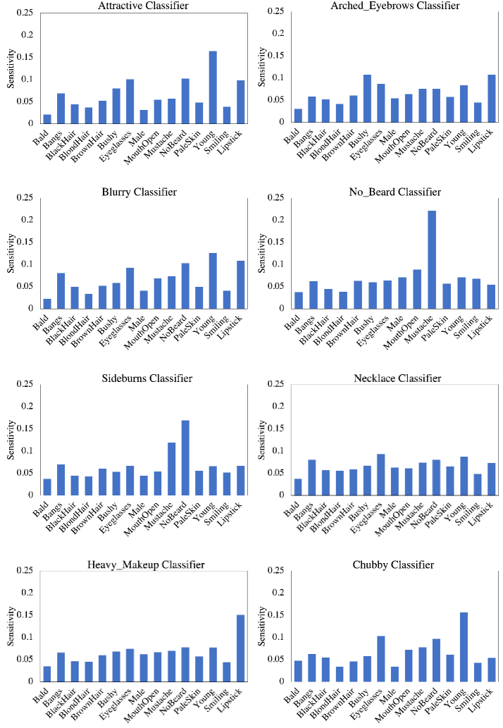
Fig. 11 shows the histograms of the sensitivity across attributes generated for additional attribute classifiers in Section 4.2.
Appendix C Image Synthesis Analysis
C.1 Visual Comparison of Adversarial Examples
Fig. 12 shows more visual comparisons of the adversarial examples generated by different methods. As we can see, SIA adds perturbation in the image space and the attribute space, generating photo-realistic fine-grained adversarial examples. Perturbing in both image space and attribute space produces finer visual adversarial images. In fact, SIA ’s pixel-level perturbation helps to avoid exaggerated semantic variation that makes the image generation collapse.
C.2 AttGAN’s Reconstruction and Semantic Editing
AttGAN () is capable of editing both fine-level semantics (e.g., beard) and complex concepts (e.g., age). The reconstruction loss during the training of guarantees the preservation of facial details. As stated in [10], the use of shortcut layers [19] improves the quality of image translation. During the SPT and SIA attack, we constrained all mutated attributes in the range of [0,1] to make sure that the transformed attribute vector for is valid. The style intensity hyper-parameter is set to , and the number of encoder layers and decoder layers are both .
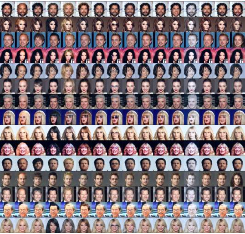
Additionally, Fig. 13 illustrates the non-adv image projection by our AttGAN backbone . We can see from the images that the inverse (flipping) attribute manipulation for most attributes is visually correct. Note that there are naturally hard cases (e.g., modifying images of people with long hair to be bold), and this can be potentially improved in future work.
Appendix D Imbalanced Datasets
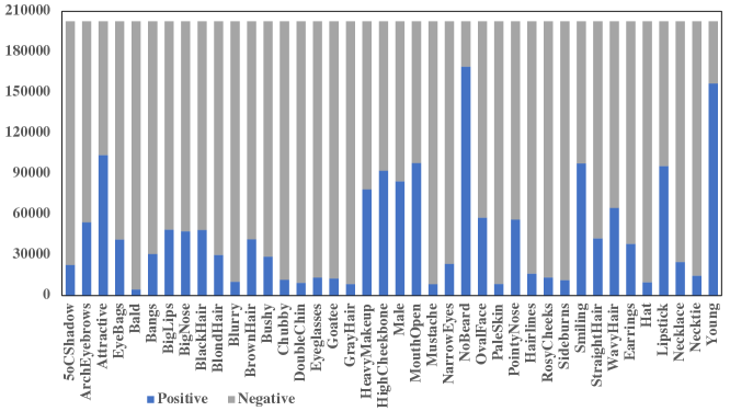
In this section, we ran data augmentation experiments using pre-trained models on a ResNet50 architecture. The pre-trained models are described in Section 4.1. Recall that the CelebA is highly imbalanced for some classes. For instance, the CelebA training set in the case of eyeglasses has Positive and Negative samples. For the bangs classifier, the imbalance in training data is Positive and Negative. As in Section 4.5, we used a balanced test data including random positive-label images and negative-label images from the CelebA test set. Table 7 shows the augmentation results on these two attributes. While SIA still beats conventional techniques in this scenario, it does so by a significantly lesser margin. Fig. 14 summarizes the label proportion of each attribute in the CelebA dataset. As we can notice, there are many attributes that are significantly unbalanced, and therefore the challenge of generating a balanced dataset across attributes.
| Eyeglasses (Pre-trained) | Bangs (Pre-trained) | |||
| F1 | Accuracy | F1 | Accuracy | |
| Non-adv classifier | 0.9789 | 97.93% | 0.9218 | 92.50% |
| Reweighting | 0.9831 | 98.33% | 0.9169 | 92.04% |
| Resample | 0.9811 | 98.15% | 0.9100 | 91.51% |
| CutMix | 0.9813 | 98.16% | 0.8993 | 90.63% |
| AutoAugment | 0.9840 | 98.42% | 0.9052 | 91.11% |
| SIA (ours) | 0.9846 | 98.48% | 0.8956 | 90.31% |
| SIA + Reweight (ours) | 0.9872 | 98.73% | 0.9285 | 93.04% |
Appendix E Attribute Sensitivity on Different Data Amount
We use SIA to evaluate the gender classifier and heavy-makeup classifiers trained with the setup in section 4.1. We take the first images from the CelebA test set and divide them into three sets of images, images, and images by data index. Note that classifiers and have never been trained on these images before. Table 8, 9, 10, 11 show the results. We can see that the sensitivities are empirically consistent over different amounts of evaluation data. To take Table 8, 9 (gender classifier) as an example, we can see that with different amounts of data the shape of the histogram (Fig. 15) remains consistent. Note that the most sensitive attribute for attacking the gender classifier is consistently the lipstick. In the open-source version, we will release the code and instructions for running SIA on multiple setups of data.
| Bald | Bangs | Black Hair | Blond Hair | Brown Hair | Bushy | Eyeglasses | Mouth Open | |
| 0.0434 | 0.0605 | 0.0405 | 0.0434 | 0.0545 | 0.0887 | 0.0803 | 0.0584 | |
| 0.0426 | 0.0580 | 0.0417 | 0.0445 | 0.0528 | 0.0879 | 0.0839 | 0.0551 | |
| 0.0427 | 0.0595 | 0.0409 | 0.0424 | 0.0532 | 0.0879 | 0.0838 | 0.0548 |
| Mustache | No Beard | Pale Skin | Young | Smiling | Lipstick | |
| 0.0755 | 0.1495 | 0.0452 | 0.0647 | 0.0370 | 0.1585 | |
| 0.0775 | 0.1493 | 0.0449 | 0.0656 | 0.0375 | 0.1586 | |
| 0.0775 | 0.1499 | 0.0458 | 0.0652 | 0.0359 | 0.1606 |
| Bald | Bangs | Black Hair | Blond Hair | Brown Hair | Bushy | Eyeglasses | Gender | Mouth Open | |
| 0.0269 | 0.0772 | 0.0438 | 0.0540 | 0.0650 | 0.0742 | 0.1296 | 0.0446 | 0.0494 | |
| 0.0268 | 0.0774 | 0.0400 | 0.0528 | 0.0631 | 0.0792 | 0.1278 | 0.0446 | 0.0525 | |
| 0.0265 | 0.0783 | 0.0419 | 0.0563 | 0.0645 | 0.0740 | 0.1294 | 0.0419 | 0.0494 |
| Mustache | No Beard | Pale Skin | Young | Smiling | Lipstick | |
| 0.0740 | 0.1244 | 0.0291 | 0.0691 | 0.0371 | 0.1016 | |
| 0.0772 | 0.1213 | 0.0298 | 0.0651 | 0.0408 | 0.1015 | |
| 0.0790 | 0.1218 | 0.0288 | 0.0679 | 0.0368 | 0.1037 |

Appendix F Attack Effectiveness
We implement SPT [11], CW [3], and Face-Manifold (FM) [14] attacks and evaluate the attack success rates (ASR) on our facial eyeglass classifier. The classifier is trained with the setup mentioned in section 4.1. For all listed setups (unless otherwise stated), the images for evaluation is the first images from CelebA test set.
In SPT attack, we use the attribute space consisting the same attributes as SIA. The optimizer is RMSProp with two learning rates and . Table 12 shows the ASR with different attack iterations. Under the same setup of iterations with , our SIA attribute-only ASR (in section 4.3 ablation study table) is 32.67% which outperforms SPT. This shows that the use of signed gradient to update the attribute space, which stabilizes the optimization, can improve the attack effectiveness.
| Iterations | 2 | 5 | 10 | 15 | 20 | 50 | 100 | 150 | 200 |
| 0.3% | 0.3% | 0.4% | 0.7% | 0.9% | 3.1% | 12.3% | 19.4% | 22.9% | |
| 1.2% | 5.0% | 14.6% | 21.7% | 25.4% | 28.3% | 29.6% | 30.3% | 29.7% |
In CW attack, we fix the attack iteration same as SIA’s and evaluate the ASR under different box-constrain parameters. Table 13 shows that by relaxing the box-constrain, the ASR can hit to 52.6% which is higher than our PGD baseline of 49.85%. The default setting of SIA where image and attribute spaces are co-updated has an ASR of 68.20% which are much more effective than CW and PGD. Note that during SIA’s adversarial optimization, we can obtain attribute sensitivity which provides intuitive model interpretation to users. Pure image space attacks cannot support such features.
| Box Contrain | 0.10 | 0.25 | 0.50 | 0.75 | 1.0 | 1.5 | 2.0 | 5.0 | 10.0 |
| ASR | 9.1% | 16.8% | 25.0% | 29.4% | 31.9% | 35.1% | 37.2% | 45.4% | 52.6% |
In FM attack, we follow the setup as specified in the original paper to make sure that we can re-implement the high ASR reported in their paper. We sample images from the style space to experiment on different settings of (style step size) and (noise step size). Table 14 shows the ASR of different and settings. We find out that noise vectors have a superior effect on flipping the prediction of our eyeglasses ResNet classifier. With increasing the strength of injected noises during the generation, the image quality will significantly decrease. Note that SIA and PGD can also achieve similar ASR (99.99% and 99.94% correspondingly) by relaxing the image space constraint.
| = 0 (no noise) | = 0.01 | = 0.02 | = 0.03 | = 0.04 | = 0.05 | |
| = 0.004 | 2.5% | 70.8% | 96.6% | 99.7% | 100.0% | 99.9% |
| = 0.01 | 2.2% | 19.3% | 55.9% | 78.8% | 91.9% | 97.3% |
| = 0.05 | 0.3% | 1.9% | 3.95% | 8.2% | 19.3% | 20.5% |
| = 0.1 | 0.2% | 0.8% | 1.3% | 2.9% | 7.0% | 12.1% |
In the open source version, we will release the code and instructions on how to set up hyperparameters, schedule baseline experiments, and run code for comparisons.


