Adversarially Contrastive Estimation of Conditional Neural Processes

Abstract

Conditional Neural Processes (CNPs) formulate distributions over functions and generate function observations with exact conditional likelihoods. CNPs, however, have limited expressivity for high-dimensional observations, since their predictive distribution is factorized into a product of unconstrained (typically) Gaussian outputs. Previously, this could be handled using latent variables or autoregressive likelihood, but at the expense of intractable training and quadratically increased complexity. Instead, we propose calibrating CNPs with an adversarial training scheme besides regular maximum likelihood estimates. Specifically, we train an energy-based model (EBM) with noise contrastive estimation, which enforces EBM to identify true observations from the generations of CNP. In this way, CNP must generate predictions closer to the ground-truth to fool EBM, instead of merely optimizing with respect to the fixed-form likelihood. From generative function reconstruction to downstream regression and classification tasks, we demonstrate that our method fits mainstream CNP members, showing effectiveness when unconstrained Gaussian likelihood is defined, requiring minimal computation overhead while preserving foundation properties of CNPs.

1 Introduction

Conditional Neural Processes (CNPs) (Garnelo et al., 2018a) are a class of neural density estimators derived from function approximation in meta-learning setting (Hospedales et al., 2021). Basically, CNPs learn an empirical prior from seen function instantiations, allowing quick adaptation to new functions within a single forward pass. Dividing each instantiation into a context and a target set, the prior is concluded as a context representation like mean function in Gaussian Processes (Williams & Rasmussen, 2006), but is parameterized by a neural network-based encoder. Using this prior, decoder generates function observations $\boldsymbol{y}_{t}$ by parameterizing a predictive distribution over all the target function covariates $\boldsymbol{x}_{t}$. Namely, CNPs are trained by exact maximum likelihood estimation (MLE). This endows CNPs with desirable properties such as tractable density and quantifiable uncertainty, suggesting them a good fit for image impainting (Kim et al., 2019), transfer learning (Gordon et al., 2020) and climate modeling (Holderrieth et al., 2021).

Tractability is indeed important, but it can also be a double-edged sword sometimes. In CNPs, the predictive distribution is conditionally factorized, which strips away correlations between samples, challenging their ability to generate coherent target observations from the predictive space (Garnelo et al., 2018b). Moreover, CNPs specify a fixed likelihood function (usually Gaussian) and assume true observations can be sampled exactly from such generative processes. The expressivity of models defined in this way is challenged when observations spanning high-dimensional spaces (Rybkin et al., 2021). Often, unconstrained Gaussian outputs fail to correctly learn correlations between dimensions and variances within each observation, leading to ill-posed MLE training (Rezende & Viola, 2018; Mattei & Frellsen, 2018).

Prior works opened up two paths in addressing the issues above. One started from latent Neural Processes (NPs) (Garnelo et al., 2018b) that introduce a latent variable to enrich the predictive space. Following, the single latent variable can be extended to hierarchical NPs to incorporate example-specific stochasticity (Wang & Van Hoof, 2020), combine function spaces of multiple tasks (Kim et al., 2021) and induce a mixture of NPs (Wang & van Hoof, 2022) to handle complicated scenarios. The latent variables, however, have intractable integrals and need to be estimated by a variational lower bound (Garnelo et al., 2018b) or Monte-Carlo approximations (Foong et al., 2020) instead. Even so, approximation does not guarantee the quality of latent representation (Alemi et al., 2018). Recently, Transformer Neural Processes (TNP) (Nguyen & Grover, 2022) flags another workaround that replaces the independent and simultaneous target predictions with an autoregressive likelihood. TNP trades off the foundational prediction consistency of CNPs in exchange for improved performance. Further, the integrated casual mask attention (Brown et al., 2020) incurs quadratic computational costs as the context size grows.

Alternatively, noise contrastive estimation (NCE) (Gutmann & Hyvärinen, 2010) has gained popularity in representation learning with complex distributions (Oord et al., 2018). Using a density ratio trick, NCE bypasses direct density estimation by learning the difference between true distribution and noise. This proves to be effective in tasks involving high-dimensional data (Chen et al., 2020; Radford et al., 2021). Previously combined with CNPs, NCE creates robust meta-representations across functions by aligning partial views of the same function and contrasting them with other functions (Gondal et al., 2021). By using self-attention (Vaswani et al., 2017), distances between covariates can further be encoded into the context representation, so as to better account for their correlations (Mathieu et al., 2021). Still, they primarily focus on learning a transferable context representation to downstream tasks and even remove the decoder from CNPs. While this motivation is also applicable as a regularization (Kallidromitis et al., 2021), no principled clue is given for how merely improving the context would benefit the generative objective of CNPs (Mathieu et al., 2021).

To fill this gap, we present a noise contrastive approach to directly calibrate the CNP predictions. Apart from the MLE objective, we provide CNPs with additional discriminative feedback evaluating if their predictions are indistinguishable from ground-truth. This prevents CNPs from solely optimizing based on inherent assumptions about data distributions. Specifically, we include an energy-based model (EBMs) (LeCun et al., 2006) learning to distinguish the true observations from those generated by CNPs. The key idea is to lift the expressivity of CNPs, which is usually restricted to a fixed form of predictive likelihood. In contrast, EBMs do not confine function form and normalized output, showing capacity to estimate complex distributions (Du & Mordatch, 2019), yet are accused of hardship in exact density estimation and sampling. Having said that, NCE suggests a principle for training EBMs to estimate an unknown distribution by discriminating between data drawn therefrom and noises from a known distribution. In this context, CNPs are ideal noise generators provided that 1) samples can be easily obtained by viewing them as prediction maps (Markou et al., 2022), and 2) density function is analytically tractable and exact.

Intuitively, we can fit such a NCE-based calibration of CNP into an adversarial training framework (Goodfellow et al., 2020). As the training progresses iteratively, CNP learns to generate increasingly realistic observations to avoid being identified easily, whereas EBM captures more discriminative characteristics in the ground-truth functions, which are then passed to CNP as gradients. It equates to approximately minimizing the Jenson-Shannon Divergence between CNP’s predictive distribution and true generative process if EBM reaches its optimality (Gui et al., 2021). In CNPs, this can be used as a regularization to complement the MLE objective.

In summary, our contributions are: i) we introduce NCE into the standard training of CNPs by adopting a flexible EBM to constrain CNP’s generative process, where EBM guides CNPs to generate predictions closer to the true observations from a discriminative viewpoint, helping to relieve ill-posed MLE training. ii) we propose integrating the joint training of EBM and CNP under an adversarial framework. The mini-max game allows EBM and CNP to be promoted iteratively, while preserving the merits of lightweight inferences by CNPs. iii) we show that the proposed approach is plug-and-play with any CNP variant, consistently improving generation performances while also facilitating downstream tasks, evaluated with both artificial and real-world datasets.

2 Preliminaries

2.1 Conditional Neural Processes

Conditional Neural Processes (CNPs) (Garnelo et al., 2018a) are parametric models that approximate stochastic processes with explicit density functions in the meta-learning setting. A stochastic process defines a family of data-generating functions $\mathcal{F}:\mathcal{X}\to\mathcal{Y}$ from covariate space $\mathcal{X}$ to an observation space $\mathcal{Y}$. Let $F$ be a collection of function instantiations sampled from the prior $p(\mathcal{F})$. We call $F$ a meta-dataset. Each instantiation $f\in F$ samples a finite sequence of covariate-observation pairs $\{(\boldsymbol{x}_{n},\boldsymbol{y}_{n})\}_{n=1:N}$ to describe a particular function mapping with noises $\xi$, such that $\mathbf{y}=f(\mathbf{x};\xi)$ with $\mathbf{x}\subseteq\mathbb{R}^{d_{\mathcal{X}}}$ and $\mathbf{y}\subseteq\mathbb{R}^{d_{\mathcal{Y}}}$. Under exchangeability and consistency required by the Kolmogorov Extension Theorem (Øksendal, 2003), the marginal joint distribution of these $N$ observations is as,

$$p(\boldsymbol{y}_{1:N}|\boldsymbol{x}_{1:N})=\int p(f)p(\boldsymbol{y}_{1:N}|\boldsymbol{x}_{1:N},f)\,\mathrm{d}f.$$ (1)

Provided a subset collection $F_{train}=\{f_{k}\}_{k=1:K}$ called meta-train set, CNPs are tasked with inferring each underlying function. For any $f_{k}$, CNPs randomly constitute a context set $D_{C}^{k}=\{(\boldsymbol{x}_{c}^{k},\boldsymbol{y}_{c}^{k})\}_{c=1:C}$ from $N$ pairs and generate observations on the target set $D_{T}^{k}=\{(\boldsymbol{x}_{t}^{k},\boldsymbol{y}_{t}^{k})\}_{t=1:T}$. Using an empirical approximation of prior $p(f_{k})$, the conditional generation of target observations is given by parameterizing a factorized predictive distribution over target covariates, with a known density likelihood (e.g., a Gaussian). Denote model parameters by $\theta$, CNPs entail a maximum likelihood estimation (MLE) within all instantiations,

$$\max_{\theta} \mathbb{E}_{f_{k}\sim F_{train}}\left[p\left(\boldsymbol{y}_{1:T}^{k}|\boldsymbol{x}_{1:T}^{k};\theta\right)\right]$$ (2)

$$= \int\prod_{t=1}^{T}p(f_{k}|D_{C}^{k};\theta)\,p(\boldsymbol{y}_{t}^{k}|\boldsymbol{x}_{t}^{k},f;\theta)\,\mathrm{d}f_{k}\,.$$

Notably, the explicit likelihood and factorized predictions ensure CNPs perform exact density estimation.

The fitted CNP model $\theta^{*}$ is then evaluated on another subset of collections called meta-test set, i.e., $F_{test}\cap F_{train}=\varnothing$. The downstream evaluation task may or may not directly relate to model training. For instance, (Garnelo et al., 2018a, b) assess the generation quality of $N$ target observations, while (Gondal et al., 2021; Mathieu et al., 2021) validate the model capacity in predicting the parameters of data-generating functions $f$ using only $C$ context samples.

2.2 Energy-based Model

Energy-based models (EBMs) (LeCun et al., 2006) are a group of density estimators with implicit density functions. Denote $\mathbf{y}$ as any i.i.d observations sampled from $\boldsymbol{y}_{1:T}$. Let $\varphi:\mathbb{R}^{d_{\mathcal{Y}}}\to\mathbb{R}$ be the energy function parameterized by an arbitrary neural network. EBMs formulate the density of $\mathbf{y}$ as a Boltzmann distribution,

$$p(\mathbf{y};\varphi)=\frac{\exp\left\{-\varphi(\mathbf{y})\right\}}{Z(\varphi)},$$ (3)

where $Z(\varphi)=\int\exp\left\{-\varphi(\mathbf{y})\right\}\mathrm{d}\mathbf{y}$ is the partition function with respect to $\mathbf{y}$, allowing $\varphi(\mathbf{y})$ to output unnormalized scalar. This flexibility in designing a neural energy function translates into the expressivity of EBMs in modeling high-dimensional data (Du & Mordatch, 2019) but also precludes direct samplings from $p(\mathbf{y};\varphi)$, typically requiring expensive and biased MCMC (Tieleman, 2008; Nijkamp et al., 2019).

As an alternative, Noise contrastive estimation (NCE) (Gutmann & Hyvärinen, 2010) has widely been adapted to learn unnormalized models like EBMs (Gao et al., 2020; Aneja et al., 2021). In principle, NCE fits EBMs to an unknown ground-truth distribution by learning to distinguish true samples from noise samples generated from a reference noise distribution. Observe $N$ samples $\boldsymbol{y}_{1:N}$ collected from a mixture of data $p_{d}(\mathbf{y})$ and noise distribution $p_{n}(\mathbf{y})$ defined with a Bernoulli indicator: $p_{d,n}(\mathbf{y})=p(v=0)p_{n}(\mathbf{y})+p(v=1)p_{d}(\mathbf{y})$. Consider an EBM, which absorbs $Z(\varphi)$ as the model’s trainable parameters, now has a normalized likelihood $p(\mathbf{y};\varphi)$. In this case, EBMs estimate the true data distribution $p_{d}(\mathbf{y})$ by training a classifier $\varphi(\mathbf{y})$ that minimizes the binary cross-entropy objective,

$$\min_{\varphi}-\left[\mathbb{E}_{\mathbf{y}\sim p_{d}(\mathbf{y})}\log\varphi(\mathbf{y})+\mathbb{E}_{\mathbf{y}\sim p_{n}(\mathbf{y})}\log\left(1-\varphi(\mathbf{y})\right)\right].$$ (4)

Essentially, EBM reaches optimality if its predictive posterior matches the true posterior $\varphi^{*}(\mathbf{y}):=p(v=1|\mathbf{y};\varphi)=p_{d,n}(v=1|\mathbf{y})$, i.e., correctly estimates the noise-data ratio of the mixture. By doing so, density estimation for EBMs can be viewed as a classification problem, assuming a noise distribution with an explicit and tractable density function.

3 Method

Our method involves implementing a joint training approach to combine CNPs with EBMs in light of their complementary attributes under the NCE framework. CNPs secure tractable and exact density estimation by locking up an explicit likelihood function by definition. In exchange, this comes at the cost of (possibly) inappropriate assumptions for observations $\mathbf{y}$ with high dimensions (Kim et al., 2021). In comparison, EBMs can be flexibly formulated in terms of network structure $\varphi$ to encompass complex distributions; yet, requiring a strong reference distribution upon performing NCE. Adversarial training (Goodfellow et al., 2020) provides an effective bridge to connect CNPs with EBMs in the NCE context, where CNP resembles the generator while EBM acts as a critic. CNP receives feedback on their generations from a discriminative perspective, while EBM also benefits from stronger predictions given by improved CNP. We now discuss a two-stage adversarial training scheme.

Figure 1: Method illustration. Stage-1) regular training of CNP $\theta$. Stage-2) calibrate CNP $\theta$ with EBM $\varphi$. 3) after training, extract context representation $\mathbf{r}_{C}$ from frozen CNP to finetune the prediction head $\phi$ for downstream tasks.

3.1 Training CNPs as a Noise Distribution

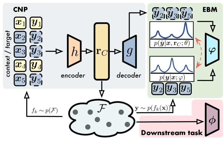
The effectiveness of NCE depends on how close the noise distribution is to the ground truth (Gutmann & Hyvärinen, 2010; Gao et al., 2020; Aneja et al., 2021): if $p_{n}(\mathbf{y})$ is too far from $p_{d}(\mathbf{y})$, EBM cannot obtain much useful information since the classifier $\varphi(\mathbf{y})$ can easily distinguish true observations from noises. It is thus crucial to train CNP to be a strong noise distribution before NCE training. For this stage, we follow the regular training of CNPs shown in Figure 1. Consider each function instantiation $f_{k}\sim F_{train}$, CNPs collapse the empirical prior $p(f_{k}|D_{C}^{k},\theta)$ into a deterministic context representation $\mathbf{r}_{C}^{k}$, approximated by a neural network-based encoder $h$ applied to the context set,

$$\mathbf{r}_{C}^{k}=\oplus_{c=1}^{C}\boldsymbol{r}_{c}^{k},\;\text{with }\boldsymbol{r}_{c}^{k}=h\left(\boldsymbol{x}_{c}^{k},\boldsymbol{y}_{c}^{k}\right)$$ (5)

where $\oplus$ is a permutation-invariant aggregate to satisfy exchangeability and consistency. Typical implementations include mean-pooling by CNP (Garnelo et al., 2018a) and self-attention by AttnCNP (Kim et al., 2019). Following, another parameterization in CNPs involves a decoder $g$ that computes sufficient statistics of the predictive distribution of each target observations $\boldsymbol{y}_{t}^{k}$, conditioned on $\boldsymbol{x}_{t}^{k}$ and $\mathbf{r}_{C}^{k}$. That is, $g$ parameterizes the mean $\boldsymbol{\mu}_{t}$ and variance $\boldsymbol{\Sigma}_{t}$ for the most heavily used Gaussian. In this sense, the parameters of CNPs $\theta=\{h,g\}$ can be optimized by MLE with a factorized exact log-likelihood over $\{\boldsymbol{y}_{1:T}^{k}\}_{k=1:K}$,

$$\max_{\theta} \mathbb{E}_{f_{k}\sim F_{train}}\left[\log p(\boldsymbol{y}_{1:T}^{k},\boldsymbol{x}_{1:T}^{k}\,;\,\theta)\right]$$ (6)

$$=\frac{1}{K}\sum_{k=1}^{K}\left\{\sum_{t=1}^{T}\log\mathcal{N}(\boldsymbol{y}_{t}^{k}|\boldsymbol{x}_{t}^{k},\mathbf{r}_{C}^{k}\,;\boldsymbol{\mu}_{t}^{k},\boldsymbol{\Sigma}_{t}^{k})\right\}\,,$$

with $(\boldsymbol{\mu}_{t},\boldsymbol{\Sigma}_{t})=g(\boldsymbol{x}_{t},\mathbf{r}_{C})$ and $\boldsymbol{y}_{t}^{k}\perp\!\!\!\perp\boldsymbol{y}_{t^{\prime}}^{k}\,|\,\mathbf{r}_{C}\;\text{for }k\neq k^{\prime}$. One can set the likelihood to other distributions depending on the dataset, e.g., Bernoulli as in (Norcliffe et al., 2021).

Upon achieving a steady low value of log probability, we consider CNP strong enough to be a noise generator. Now we begin calibrating CNP with EBM.

3.2 Calibrating CNP with EBM

Recall that our purpose is to lift the CNP’s expressivity with a flexible EBM. We do not follow (Aneja et al., 2021) where the parametric noise distribution is fixed after stage-1 training, rather in a similar way to (Gao et al., 2020) that updates the CNP and EBM parameters in an adversarial manner. One can relate the motivation here to the training in Generative Adversarial Networks: provided a powerful EBM, such as one that can estimate the density ratio correctly, means that CNP does not generate “realistic” reconstructions close enough to the real observations, and would need to be updated in order to confuse the EBM. On the other hand, CNP would only gain little cost for model improvement in the event that EBM labels the true observations as fake. As such, we can adapt the NCE objective to the joint optimization of EBM and CNP, in the way of playing a minimax game until the optimization reaches Nash equilibrium. The CNP predictions can be thought optimal if EBM can no longer identify them from true function observations.

Following a CNP forward pass with function instantiations $\{f_{k}\}_{k=1:K}$, we have $K*T$ generated observations $\dot{\boldsymbol{y}}_{1:T}^{k}$ by CNP, and $K*T$ ground-truth observations $\boldsymbol{y}_{1:T}^{k}$ over all the $K$ instantiations. We thus obtain a mixture of true data and noises to be learned from as in Equation 4. This allows us to set a noise-to-data ratio ranging from $1$ to $K$.

We let EBM and CNP iteratively maximize and minimize the posterior log-likelihood of an empirically approximated NCE objective as,

$$\min_{\theta}\max_{\varphi}$$ (7)

$$\sum_{k=1}^{K}\left\{\sum_{t=1}^{T}\log\frac{p(\boldsymbol{y}_{t}^{k}|\boldsymbol{x}_{t}^{k};\varphi)}{p(\boldsymbol{y}_{t}^{k}|\boldsymbol{x}_{t}^{k};\varphi)+p(\boldsymbol{y}_{t}^{k}|\boldsymbol{x}_{t}^{k};\theta)}\right.+$$

$$\left.\sum_{j=1}^{K}\sum_{t=1}^{T}\log\frac{p(\dot{\boldsymbol{y}}_{t}^{j}|\boldsymbol{x}_{t}^{j};\theta)}{p(\dot{\boldsymbol{y}}_{t}^{j}|\boldsymbol{x}_{t}^{j};\varphi)+p(\dot{\boldsymbol{y}}_{t}^{j}|\boldsymbol{x}_{t}^{j};\theta)}\right\}-\log K$$

where $p(\boldsymbol{y}_{t}^{(k)}|\boldsymbol{x}_{t}^{(k)};\varphi)$ and $p(\dot{\boldsymbol{y}}_{t}^{(k)}|\boldsymbol{x}_{t}^{(k)};\varphi)$ are estimated log-probabilities of true and CNP’s predictive observation at covariate $\boldsymbol{x}_{t}$ of the $k$-th function, calculated by EBM. Similarly, CNP computes log-probabilities $p(\boldsymbol{y}_{t}^{(k)}|\boldsymbol{x}_{t}^{(k)};\theta)$ and $p(\dot{\boldsymbol{y}}_{t}^{(k)}|\boldsymbol{x}_{t}^{(k)};\theta)$ of true and predicted observations accordingly. As for iterative training in practice, we set a threshold $\alpha$ to determine either EBM or CNP to be optimized, based on the accuracy of the density ratio estimated by EBM. We fix EBM and solely optimize for CNP in the case of better accuracy than $\alpha$, and vice versa.

3.3 Facilitating NCE with CNP

CNP is not the only beneficiary of adversarial training. The optimality of noise can reversely affect the performance of NCE estimator (Chehab et al., 2022). All throughout training, CNP provides the MLE estimate of noise parameters thanks to the exact density likelihood. Using the estimate of noise distribution is shown to be helpful in reducing the asymptotic variance of NCE (Uehara et al., 2018).

Meanwhile, the large batch training required by previous contrastive learning models (Oord et al., 2018; Chen et al., 2020) may also be appreciated in this setting. Note that the summation from $1$ to $K$ with the second term inside brackets in Equation 7 means that we can get negative samples from the CNP’s predictions of other $K-1$ functions. While NCE could theoretically reach Cramér-Rao bound with an infinitely large batch size (Gutmann & Hyvärinen, 2012), it is computationally infeasible. However, one can also set this noise-to-data ratio to $1$ following common practices, i.e., some proportion for true observations and noises. With the predictions of CNP, this can be touched by only contrasting the ground-truth to predictions within the same instantiation.

3.4 Regularizing MLE with NCE

Following the results of (Goodfellow et al., 2020), prior works (Gao et al., 2020; Aneja et al., 2021) connect the NCE objective in Equation 7 to an approximate minimization of Jensen-Shannon (JS) divergence between true distribution of observations $p(f(\mathbf{x}))$ and predictive density of CNP $p(\mathbf{y}|\mathbf{x};\theta)$ when updating $\theta$,

$$D_{JS}\left(p(\mathbf{y}|\mathbf{x};\theta)\,||\,p(f(\mathbf{x}))\right)=\left[\varphi^{*}(\mathbf{y})-\log(4)\right]/\,2\,,$$ (8)

provided that EBM is the optimal $\varphi^{*}$, i.e., the density of EBM equals to ground-truth $p(\mathbf{y}|\mathbf{x},\varphi^{*})=p(f(\mathbf{x}))$. This may suggest that if the minimax game is successfully played, NCE could facilitate the estimation of CNP other than simply optimizing the KL-divergence as in MLE objective.

Yet, we find that the performance of CNP is empirically hindered if we fully turn to Equation 7 (Appendix G). Thus, we derive a more practical objective in implementations by weighting Equation 6 with Equation 7. Denote the equivalent loss of Equation 6 to $\ell_{1}(\theta)$ and Equation 7 to $\ell_{2}(\varphi,\theta)$, we conclude the loss function in stage-2 as $(1-\beta)\cdot\ell_{1}(\theta)+\beta\cdot\ell_{2}(\varphi,\theta)$, where $\beta$ is the trade-off coefficient. To this extent, we can view NCE as an auxiliary objective of MLE optimization of CNPs.

3.5 Downstream Tasks Transfer

While the post-training capability of context representations has not been extensively evaluated in the CNPs literature, this appears to be another interest metric as discussed in (Gondal et al., 2021; Mathieu et al., 2021). In this paper, we consider the supervised finetuning evaluations on the meta-test set $F_{test}$. Assume each sample in $F_{test}$ is of the form $(f_{e},l_{e})$. Each instantiation has an associated label. For example, in the case of Motor Imagery recognition with electroencephalography (EEG) signals. Let $f_{e}$ be a recorded EEG clip recorded when a subject is performing a particular imagination class $l_{e}$ (e.g., imaging making a fist with the left hand). Using a pre-trained CNP with frozen parameters $\theta^{*}$, we extract the context representation $\mathbf{r}_{C}$ from the context set, and input it to the prediction head $\phi(\mathbf{r}_{C}):\mathbb{R}^{d_{r}}\to\mathbb{R}^{d_{l}}$. The prediction head follows standard supervised optimization. In this sense, training CNPs can be seen as self-supervised representation learning. Code is available at Footnote 3.

4 Related Work

Conditional Neural Processes (CNPs). CNPs were proposed to bridge the expressivity of neural networks and the fast adaptability of non-parametric models, defining their inference as encoding context samples, aggregation, and decoding over target samples with a factorized predictive distribution. As CNP (Garnelo et al., 2018a) does not consider any correlations between samples, the subsequent works aim to improve model expressivity. The CNPs members contribute to leveraging distances between samples. AttnCNP (Kim et al., 2019) uses self-attention within context set and cross-attention with respect to each target point to account for absolute distances between covariates. Thereafter, ConvCNP (Gordon et al., 2020) and SteerableCNP (Holderrieth et al., 2021) introduce symmetries into CNPs, namely translation equivariance and group equivariance, respectively. Another family relating to CNPs has evolved since (Garnelo et al., 2018b), latent NPs members replace (or append to) the deterministic inference of CNPs with latent variables to capture the global uncertainty of data-generating processes and transform the predictive distribution into an infinite mixture of Gaussian. Further works draw inspiration from hierarchical generative models and equip NPs with increasingly powerful latent hierarchies (Kim et al., 2021; Wang & van Hoof, 2022). Yet, improved capacity also comes with a cost of intractable likelihood. One needs to apply a variational lower bound (Garnelo et al., 2018b; Kim et al., 2019) or repeat Monte Carlo approximations (Foong et al., 2020) to derive the approximated log-likelihood. Recently, TNP (Nguyen & Grover, 2022) applies a casually-masked transformer to accommodate sequential data, introducing autoregressive predictions to NPs. Instead of presenting a new variant of CNPs, our work discusses a general calibration principle with adversarial training, which is compatible with any CNP member. Our method neither alters CNP’s original inference procedure nor burdens it with heavy computation overhead.

Function Contrastive Representation Learning (FCRL). CNPs had previously combined noise contrast estimation (NCE) in the spirit of contrastive self-supervised learning. Inspired by MetaCDE (Ton et al., 2021), FCRL (Gondal et al., 2021) pursues a robust meta-representation space for context set, where partial views of the same function are pulled closer while different functions are pushed away. CReSP (Mathieu et al., 2021) replaces the mean-pooling of context representation with self-attention. While FCRL and CReSP entirely discard generation and prioritize downstream tasks where reconstruction is unnecessary, NCE optimization may be used as regularization to the generation (Kallidromitis et al., 2021; Ye & Yao, 2022). Still, these practices do not address the question, as to how context representations can be improved to facilitate generation. Despite also using NCE, our motivation differs from all these works as we directly calibrate the CNPs’ generation. We consider the predictive distribution to be noise in NCE and refine CNP with a more flexible unnormalized estimator.

Energy-based Models (EBMs). EBMs are arguably flexible statistical models in terms of their unconstrained function form and unnormalized output. The expressive power of EBMs is demonstrated in recent connections to deep models (Du & Mordatch, 2019). A compositional nature is also evident when EBMs are combined with explicit generative models such as variational autoencoders (VAEs) (Kingma & Welling, 2013). VAEs can be taught a prior distribution with EBMs empowered by implicit generation (Pang et al., 2020; Xiao et al., 2020; Aneja et al., 2021). Yet, the downside of these approaches involves expensive MCMC sampling with high-dimensional data. To avoid implicit sampling, NCE is widely studied for estimating EBMs by separating ground-truth data density from some sample-efficient reference distributions referred to as noise. It is primarily important to find an appropriate noise distribution. Conditional NCE (Ma & Collins, 2018) generates noises with observed true data. Bose et al. propose an adversarially learned sampler from the mixture of true data and noise (Bose et al., 2018). Our work takes a similar spirit to (Gao et al., 2020), where EBMs are applied to help the estimation of a normalization flow of true data. In contrast, our work is devoted to learning a prediction map in the meta-learning setting, where noise samples can be obtained via a single forward pass of CNPs.

5 Empirical Studies

We plug the proposed method into a range of CNP variants to justify the performance change before and after adversarial calibration. We evaluate the model capacity in terms of generation performances (as in most CNPs literature; Section 5.1) and the transferability of context representations to four downstream tasks (Section 5.2). Both evaluations involve synthesized and real-world data. Our interests fall into two central questions: (1) Does adversarial training with noise contrastive estimation improve the generation performance of CNPs? (2) If so, does improved generation ability promote downstream tasks such as classification?

5.1 Generation

5.1.1 Synthesized 1D Data Regression

Table 1: The regression MSE ($\downarrow$) on synthetic 1D GP functions, sine waves, and damped oscillators$(\times 10^{-1})$. Bold indicates adversarial training leads to performance improvement over the original CNP model. Results are mean $\pm$ std with three different seeds.

Method	GP-RBF	Sinusoid	Oscillator
CNP	2,873 $\pm$ 0.162	0.795 $\pm$ 0.151	0.246 $\pm$ 0.029
ACNP	1.829 $\pm$ 0.117	1.138 $\pm$ 0.062	0.697 $\pm$ 0.067
CCNP	2.185 $\pm$ 0.072	0.459 $\pm$ 0.026	0.596 $\pm$ 0.133
CNP-adv	2.107 $\pm$ 0.096	0.481 $\pm$ 0.042	0.183 $\pm$ 0.025
ACNP-adv	1.507 $\pm$ 0.192	0.987 $\pm$ 0.073	0.711 $\pm$ 0.081
CCNP-adv	2.093 $\pm$ 0.015	0.389 $\pm$ 0.042	0.221 $\pm$ 0.022

Setup. We first consider a few-shot regression with 1D synthetic data generated by Gaussian Processes (GPs) with RBF kernels, and 1D functions generated by closed-form expressions of sine waves and damped oscillators. For GP-RBF data, we randomly generate 4,096 functions for meta-train, and 1,000 functions for meta-test. Each function instantiation has 128 points. In training, the context set is randomly sampled from $\mathcal{U}[0.1,0.3]$, all 128 points are used as the target set, while in evaluation, the context size is fixed to 0.3. As for sine waves and oscillators, we set the meta-train functions and meta-test functions to 500, where each instantiation has 100 points. As well, the context size is between $[0.04,0.2]$ during training and is fixed to $0.2$ in evaluation. For sine waves, we vary the values of amplitude $\mathcal{U}[-1,1]$ and shift within $\mathcal{U}[-0.5,0.5]$, covariates $x\in[-3\pi,3\pi]$. Each oscillator function has a unique amplitude and shift $a\sim\mathcal{U}[-3,3]$ and $b\sim\mathcal{U}[-1,1]$, with $x$ starting at $0$ and going up to $5$. See full details of the setup in Appendix B.

Results. Table 1 presents the quantitative results of various baseline CNPs with and without adversarial training. The baseline models include CNP (Garnelo et al., 2018a), ACNP (Kim et al., 2019), and CCNP (Kallidromitis et al., 2021), where the first two are commonly adopted as per most CNPs literature. We consider CCNP as a comparison to the previous NCE setting, where NCE is also applied but on the context set as a regularization term to CNPs.

We find that adversarial training consistently results in performance improvements to baselines in most cases. Notably, while ACNP is arguably more powerful than CNP and indeed reports better results as expected for GP data (Kim et al., 2019), it performs worse with sine and oscillator data, probably due to the number of functions being too limited. Also, CCNP does not improve CNP consistently either. Further, we observe that adversarial training can be adapted to CCNP, showing potential in improving generative CNPs by leveraging composite contrastive objectives.

5.1.2 Basketball Trajectory Imputation

Table 2: The test likelihoods comparison ($\uparrow$) with basketball game trajectories, without and with adversarial training. Results are with three different seeds, improved results are in bold.

	CNP	CCNP	ACNP
w/o adv	-26.266 $\pm$ 8.126	-3.457 $\pm$ 2.456	216.268 $\pm$ 0.5026
w/ adv	-0.947 $\pm$ 1.961	17.304 $\pm$ 4.277	221.016 $\pm$ 2.771

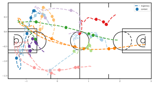
Setup. We next investigate a real-world trajectory dataset, the STATS SportsVU tracking data from the 2012-2013 NBA season (Lucey et al., 2014). Each sequence describes the movements of 10 players and the ball with respect to their coordinates on the court, lasting for 50 timesteps. We are tasked with imputing the observation of the coordinates at each timestep, where each observation is of dimension $\mathbf{y}\in\mathbb{R}^{22}$. The meta-train set and meta-test contains 104,003 and other 13,464 sequences, respectively. For each batch during training, the context size is randomly sampled $\mathcal{U}[0.1,0.5]$ whilst using all 50 frames as the target set. The context size in evaluation is fixed to $0.5$. We predict the outcome with diagonal multivariate normal distribution because in basketball games all players take action in relation to the ball. More details are covered in Appendix C.

Results. Observe that adversarial training consistently impacts all CNP variants positively from Table 2, especially for CNP and CCNP. By introducing adversarial training, the predictive likelihoods of CNP and CCNP improve by orders of magnitude over the original model, from $-26.27$ to $-0.95$ and $-3.46$ to $17.30$, respectively. CCNP regularizes CNP with NCE by pairing different partial views of each function, we find that adversarial training further improves the results of CCNP. ACNP significantly outperforms the other two CNP variants with and without adversarial training thanks to the attention mechanism. Nevertheless, it is possible for ACNP to be overconfident in its predictions (Nguyen & Grover, 2022). Such cases may not benefit ACNP as much as CNP and CCNP from adversarial calibration.

5.1.3 Image Sequence Reconstruction

Figure 2: The qualitative comparison with bouncing ball data. The showcased frames are irregularly sampled within one sequence.

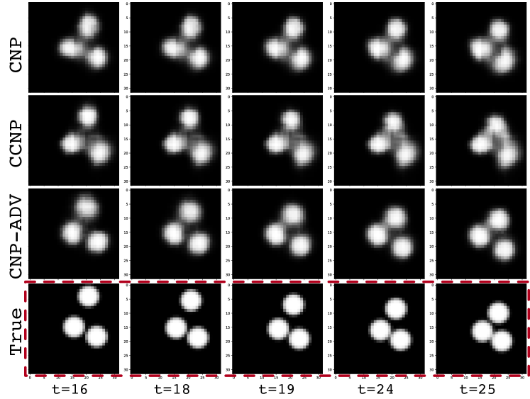
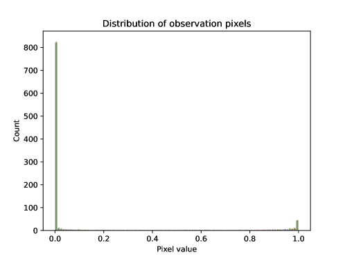
Setup. The third generation task involves reconstructing irregularly sampled high-dimensional sequences of images (Yildiz et al., 2019). The dataset describes a bouncing ball system with three interacting balls moving within a rectangular box. Each sequence contains 50 frames of $32\times 32$ grayscale images. The meta-train set has 10,000 sequences while we use another 500 sequences in meta-test set. We randomly sample the context size from $\mathcal{U}[0.1,0.5]$ during training and fix that to 0.5 for evaluation. Following (Norcliffe et al., 2021), we set the predictive likelihood to diagonal Bernoulli since most of the pixel intensities are located around $0$ and $1$. We include the full details in Appendix D.

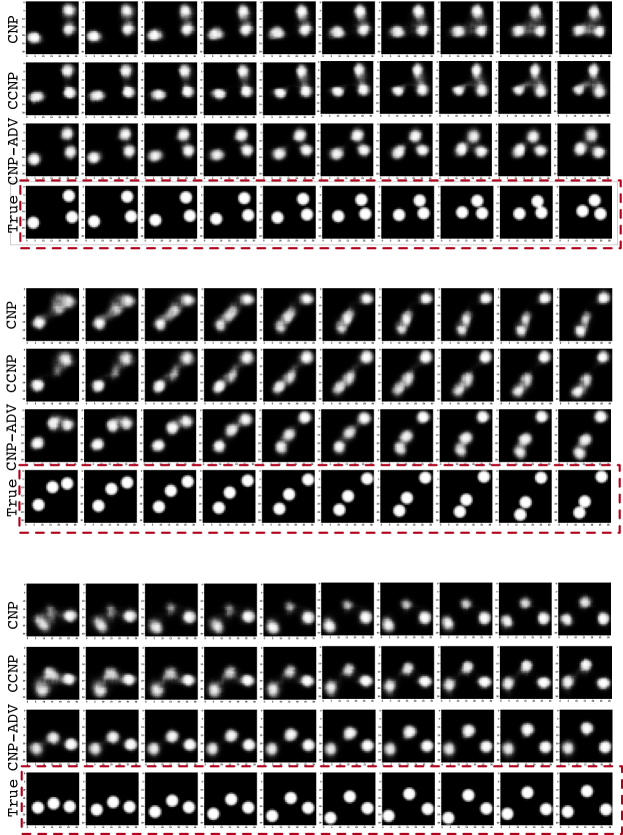
Results. Figure 2 qualitatively compares the generation results of CNP, CCNP (i.e., with NCE regularization), and CNP-adv (i.e., with adversarial training). As seen from the first and the second rows, CNP and CCNP cannot cope with frames where three balls are gathered closely. The reconstructions are blurry, and even balls cannot maintain the shape in, e.g., $t=24,25$. In contrast, CNP-adv generates better-quality images. Meanwhile, we directly evaluate the effects of adopting NCE with adversarial training or as regularization to the context set. We thus conclude that NCE combined with adversarial calibration improves the capability of CNP in reconstructing high-dimensional observations.

5.2 Downstream Tasks

In this section, we evaluate if NCE indeed helps with the transferability of context representations. The pre-trained CNPs are used as self-supervised feature extractors (parameters are frozen), followed by a trainable prediction head $\phi(\cdot)$ upon performing supervised downstream prediction tasks.

5.2.1 Function Parameter Inference

(a) Oscillator amplitude $a$

(b) Oscillator shift $b$

Figure 3: The prediction MSE (mean$\pm$std) $\downarrow$ of 1D function parameter inference on Oscillator data, with different context sizes.

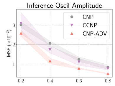
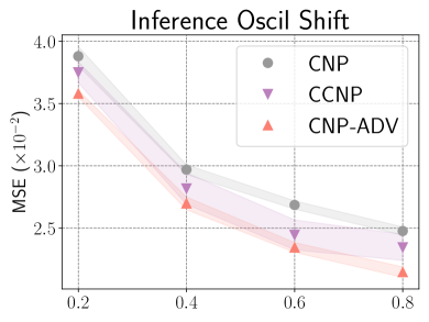
Setup. For the CNPs trained with the oscillator dataset in Section 5.1.1, we append a prediction head to infer the amplitude $a$ and shift $b$. Given some context points, the task is to identify a specific $a$ and $b$ used to generate the function. The downstream predictions sample random context points in a fixed number for both training and testing. The best-performing CNPs of each run are used. The prediction head is trained for 20 epochs. Appendix B covers a detailed setup.

Results. While CNPs are pre-trained with the context size $\mathcal{U}[0.04,0.2]$, they can handle varied numbers of context points in evaluation. Figure 3 depicts the regression MSE with different context size ranging from $0.2$ to $0.8$. More context points lead to improved prediction performances for all the CNP, CCNP, and CNP-ADV. Both CCNP and CNP-ADV include NCE, shown to help CNP identify the underlying function parameter. Although this is a typical use case of improving the context set with NCE (Gondal et al., 2021), we observe that CNP-adv consistently outperforms CCNP, even without focusing on the context set particularly.

5.2.2 Motor Imagery Classification

People-centric sensing can be an important real-world application of CNPs, where the recordings are naturally noisy and contain missing values frequently.

Setup. We predict the associated motor imagery task based on irregularly sampled Electroencephalography (EEG) measurements (Goldberger et al., 2000). The dataset contains 64-channeled EEG recordings of 105 subjects performing various motor imagery tasks. We perform binary classification regarding if opening and closing both fists or feet. EEG clips are 4 seconds long with 640 timesteps. The context size is sampled from $\mathcal{U}[0.5,0.8]$ during CNP training. We split all the clips of 105 subjects with a ratio of 3,746/400/400 clips in train/validation/test sets. The prediction head is trained for 10 epochs. See Appendix E for more details.

Table 3: The prediction accuracy with EEG Motor Imagery dataset.

	CNP	CCNP	CNP-ADV
MSE($\downarrow$)	1.99 $\pm$ 0.24	1.78 $\pm$ 0.44	1.68 $\pm$ 0.16
ACC($\uparrow$)	66.46 $\pm$ 1.40	65.18 $\pm$ 1.90	70.43 $\pm$ 0.78

Results. Similarly, both CCNP and CNP-ADV contribute to more accurate reconstruction of EEG measurements. However, CCNP appears to perform worse in the Motor Imagery classification task. In this case, the increased reconstruction ability does not necessarily lead to a context representation that facilitates downstream tasks, which is aligned with (Gondal et al., 2021). While CCNP draws the motivation therefrom, the NCE adopted on context set does not clearly demonstrate effectiveness in practice. A possible reason is, the number of functions (3,746) might be insufficient to express the capacity of self-supervised contrastive learning. In contrast, CNP-ADV decreases the reconstruction MSE while also increasing the classification accuracy. Accordingly, the adversarial calibration of CNPs with NCE could benefit both reconstruction and downstream tasks.

5.2.3 Human Activity Recognition

Setup. We lastly evaluate the activity recognition capacity with PAMAP2 (Reiss & Stricker, 2012), another sensor-based people-centric dataset that contains records of 8 subjects upon performing 4 different physical activities, with 3 inertial measurement units (IMU). Each IMU records 12 effective features per timestep. The activity labels contain Following mild preprocessing, e.g., drop invalid values and apply sliding windows, we obtain 50 timesteps times with $\mathbf{y}\in\mathbb{R}^{36}$ for each sequence. The context size subjects to $\mathcal{U}[0.5,0.7]$ during training. For each run, we select 2 subjects for validation and testing. The remaining 6 subjects are used for pre-training CNPs and then training the prediction head. This results in around 9,600 training, 1,600 validation and 1,600 testing sequences. The prediction head is trained for 10 epochs. Appendix F covers more details of the setup.

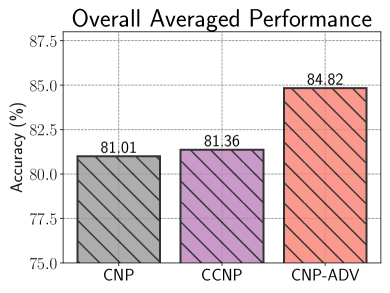
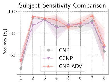
Results. Human activities manifest inter-subject variability. That is, different patterns may emerge even when subjects perform the same cognitive task. We thus report the average overall comparison (Figure 4(a)) and subject-specific comparisons (Figure 4(b)). While CCNP achieves higher average accuracy than CNP, it performs worse with a range of subjects. In comparison, CNP-ADV consistently improves CNP with almost all subjects. Even with subject #1 and #8 who have distinct activity patterns from others, CNP-ADV yields better prediction results than both CNP and CCNP.

(a) Average Acc of 8 subjects

(b) Subject-specific Acc

Figure 4: The prediction accuracy of PAMAP activity recognition.

5.3 Complexity Overhead

We have discussed that adversarial calibration benefits the expressivity of CNPs in terms of both generation and downstream tasks. We also claim that it does not impose a heavy computational burden on the original CNP model. It does not alter how CNPs perform a complete training step and how CNPs make inference. The additional computation with respect to Equation 7 is embarked by EBM that takes CNP predictions and true observations over all target points. Still, the complexity is determined by the original CNP variant. For example, the asymptotic complexity of CNP is increased from $O(C+T)$ to $O(C+T+2*T)$, but not enlarging its order. We include more empirical comparisons of relative training time and memory consumptions in Appendix H.

6 Discussion and Future Overlook

Summary. We presented an adversarial training scheme for calibrating the predictions of CNPs with NCE. The expressivity of CNPs can be improved with a simple yet effective adversarial calibration process, by training a flexible unnormalized EBM that distinguishes true observations from ones generated by CNPs in the principle of NCE. This provides a discriminative objective, by which CNPs must learn to fool EBM rather than simply following the pre-defined maximum likelihood estimate. Our study demonstrated that CNPs would benefit more from NCE in adversarial training than from previous settings focusing on context representations, in terms of both generation and downstream tasks.

Limitation and Future Extension. One limitation of this study is introduced by the pre-defined likelihood function of CNPs. Despite adversarial training helping with predictions of CNPs, the function forms of factorized predictive distributions remain unchanged. Combining this with tractable distribution transformation approaches, such as normalizing flows (NFs), may provide a solution. It is not trivial since NFs could challenge the consistency of CNPs as discussed in (Markou et al., 2022). Another solution might be applying adversarial training to latent NPs, since they have a more flexible predictive space than CNPs. However, it is unclear whether the NCE objective is directly applicable as latent NPs can only be estimated with approximated likelihoods.

Appendix A Consistency and Exchangeability

Two foundation properties of CNPs are exchangeability and consistency under permutations and marginalization to satisfy the Kolmogorov Extension Theorem (Øksendal, 2003). We next show that CNPs in adversarial training with NCE (CNPs-ADV) do not violate such properties.

Suppose a data-generating function $f(\mathbf{x})$ with a list of target input $\boldsymbol{x}_{1:T}=\{\boldsymbol{x}_{t}\}_{t=1:T}$ have corresponding output $\boldsymbol{y}_{1:T}=\{\boldsymbol{y}_{t}\}_{t=1:T}$. Denote a random subset of target by $D_{C}:=\{\boldsymbol{x}_{c},\boldsymbol{y}_{c}\}_{c=1:C}\subset\{\boldsymbol{x}_{t},\boldsymbol{y}_{t}\}_{1:T}$. Let $\rho_{T}$ be any permutation of $\{1,\dots,T\}$ and $\rho_{C}$ be any permutation of $\{1,\dots,C\}$. Consider a CNP $\theta:=\{h(D_{C}),g(\boldsymbol{x}_{t},p(f))\}$ and an EBM $\varphi(\cdot)$.

Lemma A.1.

For any covariate $\boldsymbol{x}_{t}$, the output of EBM $\varphi(\cdot)$ is an injective composition $\varphi\circ f:\mathbb{R}^{d_{\mathcal{Y}}}\to\mathbb{R}$ of a function $f(\mathbf{x})$.

Proof.

An EBM $\varphi(\cdot)$ takes either true observation $\boldsymbol{y}_{t}=f(\boldsymbol{x}_{t})$ or predictive observation $\dot{\boldsymbol{y}}_{t}=g(\boldsymbol{x}_{t},p(f))$ as input. This holds in the fact that CNP collapses $p(f)$ into a deterministic tensor $\mathbf{r}_{C}$ given $D_{C}$, and the decoder $g$ is a function of $\boldsymbol{x}_{t}$. ∎

Proposition A.2.

CNPs-ADV satisfy the exchangeability under any permutations.

Proof.

The joint marginal distribution over $\boldsymbol{x}_{1:T}$ parameterized by a CNP $\theta$ is permutation-invariant to $\rho_{T}$ given by,

$$p(\boldsymbol{y}_{1},\dots,\boldsymbol{y}_{T}|\boldsymbol{x}_{1},\dots,\boldsymbol{x}_{T}) =\int p(f)p(\boldsymbol{y}_{1},\dots,\boldsymbol{y}_{T}|\boldsymbol{x}_{1},\dots,\boldsymbol{x}_{T},p(f))\,\mathrm{d}f$$ (9)

$$\approx p(\boldsymbol{y}_{1},\dots,\boldsymbol{y}_{T}|\boldsymbol{x}_{1},\dots,\boldsymbol{x}_{T},\boldsymbol{x}_{1},\dots,\boldsymbol{x}_{C},\boldsymbol{y}_{1},\dots,\boldsymbol{y}_{C};\theta)$$

$$=p(\boldsymbol{y}_{1},\dots,\boldsymbol{y}_{T}|\boldsymbol{x}_{1},\dots,\boldsymbol{x}_{T},\mathbf{r}_{C};\theta)$$

$$=\prod_{t=1}^{T}p(\boldsymbol{y}_{t}|\boldsymbol{x}_{t},\mathbf{r}_{C};\theta)\qquad\text{assume }p(\boldsymbol{y}_{t}|\boldsymbol{x}_{t};\theta)\perp\!\!\!\perp p(\boldsymbol{y}_{t^{\prime}}|\boldsymbol{x}_{t};\theta)\mid\mathbf{r}_{C},\;\forall\;t\neq t^{\prime}$$

$$=\prod_{t=1}^{T}p(\boldsymbol{y}_{\rho_{T}(t)}|\boldsymbol{x}_{\rho_{T}(t)},\mathbf{r}_{C};\theta)$$

$$=p(\boldsymbol{y}_{\rho_{T}(1)},\dots,\boldsymbol{y}_{\rho_{T}(T)}|\boldsymbol{x}_{\rho_{T}(1)},\dots,\boldsymbol{x}_{\rho_{T}(T)})$$

provided that

$$\mathbf{r}_{C} =\oplus_{c}\,h(\boldsymbol{x}_{c},\boldsymbol{y}_{c})=\oplus_{\rho_{c}(c)}\,h(\boldsymbol{x}_{\rho_{c}(c)},\boldsymbol{y}_{\rho_{c}(c)}),\qquad\forall\,c\in 1,\dots,C$$ (10)

such that $\mathbf{r}_{C}$ is invariant to $\rho_{C}$ if $\oplus$ is a permutation-invariant aggregation operation, e.g., mean-pooling (Garnelo et al., 2018a) and self-attention (Kim et al., 2019).

With Lemma A.1, the EBM outputs an injective $\varphi\circ f$ of $p(\boldsymbol{y}_{t}|\boldsymbol{x}_{t},\mathbf{r}_{C},\theta)$ which is parameterized by $\dot{\boldsymbol{y}_{t}}$. The permutation $\rho_{T}$ on $\{1,\dots,T\}$ thus has an unique consequence on $\varphi(\dot{\boldsymbol{y}}_{\rho_{T}(t)})$

$$\varphi(\dot{\boldsymbol{y}}_{1}),\dots,\varphi(\dot{\boldsymbol{y}}_{T})=\varphi(\dot{\boldsymbol{y}}_{\rho_{T}(1)}),\dots,\varphi(\dot{\boldsymbol{y}}_{\rho_{T}(T)})$$ (11)

The same holds for $\varphi(\boldsymbol{y}_{\rho_{T}(t)})$. ∎

Proposition A.3.

CNPs-ADV satisfy the consistency under marginalization.

Proof.

Given the conditional independence assumption within target, marginalizing out $\boldsymbol{y}_{1},\dots,\boldsymbol{y}_{T-1}$ results in the joint predictive distribution of $\boldsymbol{x}_{1},\dots\boldsymbol{x}_{T}$ as

$$\int\dots\int p(\boldsymbol{y}_{1},\dots,\boldsymbol{y}_{T}|\boldsymbol{x}_{1},\dots,\boldsymbol{x}_{T},\mathbf{r}_{C};\theta)\,\mathrm{d}\boldsymbol{y}_{1}\dots\mathrm{d}\boldsymbol{y}_{T-1}$$ (12)

$$= \int\dots\int p(\boldsymbol{y}_{T}|\boldsymbol{x}_{T},\mathbf{r}_{C};\theta)p(\boldsymbol{y}_{1},\dots,\boldsymbol{y}_{T-1}|\boldsymbol{x}_{1},\dots,\boldsymbol{x}_{T-1},\mathbf{r}_{C};\theta)\,\mathrm{d}\boldsymbol{y}_{1}\dots\mathrm{d}\boldsymbol{y}_{T-1}$$

$$= p(\boldsymbol{y}_{T}|\boldsymbol{x}_{T},\mathbf{r}_{C};\theta)\int p(\boldsymbol{y}_{1}|\boldsymbol{x}_{1},\mathbf{r}_{C};\theta)\,\mathrm{d}\boldsymbol{y}_{1}\int\dots\int p(\boldsymbol{y}_{T-1}|\boldsymbol{x}_{T-1},\mathbf{r}_{C};\theta)\,\mathrm{d}\boldsymbol{y}_{T-1}$$

$$= p(\boldsymbol{y}_{T}|\boldsymbol{x}_{T},\mathbf{r}_{C};\theta)$$

As the density of $\dot{\boldsymbol{y}}_{T}$ remains unchanged depending on $\boldsymbol{x}_{t}$ and $\mathbf{r}_{C}$. Resembling the exchangeability condition, the injective $\varphi\circ\dot{\boldsymbol{y}}_{T}$ does not violate the consistency requirement held by CNP. ∎

Appendix B Additional Details for 1D Data.

B.1 Experiment Setup

B.1.1 Dataset Description

(a) Examples of sine wave functions

(b) Examples of oscillator functions

Figure 5: Examples of 1D functions used in the experiment.

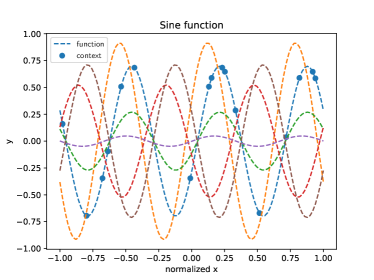
The sine wave functions are generated by

$$y=a*\sin(x-b),\quad\text{with }a\sim\mathcal{U}[-1.0,1.0],\text{ and }b\sim\mathcal{U}[-0.5,0.5],$$ (13)

where $\mathbf{x}$ are evaluated from $[-3\pi,3\pi]$.

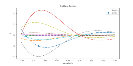
The damped oscillator functions are generated by

$$y=a*\exp(-0.5x)*\sin(x-b),\quad\text{with }a\sim\mathcal{U}[-3.0,3.0],\text{ and }b\sim\mathcal{U}[-1.0,1.0],$$ (14)

where $\mathbf{x}$ are evaluated from $[0,5]$. Both function families have 100 points per instantiation. The train/validation/test set has distinct 500 instantiations, respectively.

For Gaussian Processes (GP) generated data, we adopt a commonly-used RBF kernel

$$k\left(\mathbf{x},\mathbf{x}^{\prime}\right)=\exp\left(-\frac{\left\|\mathbf{x}-\mathbf{x}^{\prime}\right\|^{2}}{2\sigma^{2}}\right),\quad\text{with }\sigma=0.2.$$ (15)

where $\mathbf{x}$ are evaluated from [-1., 1.] at 128 uniformly spacing covariates. The train/set has 4,096 and 1,000 instantiations, respectively.

For each dataset, the covariate range $\mathbf{x}$ is linearly scaled to $[-1,1]$ regardless of their original lower and upper bound.

B.1.2 Setup

CNPs Training. We use all the points of a function instantiation as the target size throughout this work. We fix context size in evaluation to the upper bound of that in training. For other datasets, these remain the same unless explicitly stated.

• context size: $\mathcal{U}[0.04,0.2]$ for sine and oscillator functions; $\mathcal{U}[0.1,0.3]$ for GP-RBF functions.

• batch size: 16 for sine and oscillator functions; 128 for GP-RBF functions.

• episodes: 200 for sine and oscillator functions; 250 for GP-RBF functions.

• optimization: Adam with learning rate 1e-3. Weight decay 6e-5.

CNPs-Adv Training. To calibrate CNPs predictions with NCE, we append an EBM following each original CNP variant. Within each batch of $B\times T$ target points, EBM takes both $B\times T$ true observations and $B\times T$ predicted observations as input, and outputs a scalar value for each input. The training of CNPs-Adv is in two stages. In stage 1, we train CNPs as usual, until the validation loss does not decrease in 20 consecutive epochs. In stage 2, we put EBM into joint training. We obtain a value with respect to Equation 7 and compute the prediction accuracy of EBM on the density ratio. If the accuracy is greater than the threshold $\alpha$, then update CNP in the next batch, otherwise update EBM (with another optimizer).

• iterative threshold $\alpha$: 0.6.

• optimization: Adam with learning rate 7e-4

Downstream Task Training. We fix the parameters of pre-trained CNPs $\theta^{*}$, and use a prediction head $\phi(\mathbf{r}_{C})$ on the context representation extracted by CNPs $\theta^{*}$.

The downstream regression task involves only oscillator functions. We are tasked with predicting the amplitude $a$ or the shift $b$ given a particular function instantiation, i.e., $\phi:\mathbb{R}^{d_{r}}\to\mathbb{R}$.

• context size: 0.2

• batch size: 32

• Episodes: 20

• Optimization: Adam with learning rate 5e-4. Weight decay 6e-5.

B.2 Model Implementation

We provide the implementations for 1D and basketball data in.

In practice, both covariates $\boldsymbol{x}$ and observations $\boldsymbol{y}$ can be multi-dimensional, i.e., $d_{\mathcal{X}}>1,d_{\mathcal{Y}}>1$. Thus, we follow the interpretation of (Mathieu et al., 2021) that applies a covariate network (CovNet) and an observation network (ObsNet) to pre-transform covariates and observations into features, such as a CNN to process image observations $\boldsymbol{y}$ with $d_{\mathcal{Y}}=1024$.

B.2.1 CNP

Sine and oscillator.

• CovNet: identity $\mathbb{R}\to\mathbb{R}$

• ObsNet: identity $\mathbb{R}\to\mathbb{R}$

• Encoder $h(\boldsymbol{x},\boldsymbol{y})$: 2-(hidden) layer MLP $\mathbb{R}^{2}\to\mathbb{R}^{64}$, with hidden size $[64,64]$.

• Aggregator: mean-pooling

• Decoder $g(\boldsymbol{x},\mathbf{r}_{C})$: 2-layer MLP $\mathbb{R}^{65}\to\mathbb{R}$, with hidden size $[64,64]$.

• Likelihood: diagonal Gaussian with event shape $1$.

GP-RBF.

• CovNet: identity $\mathbb{R}\to\mathbb{R}$

• ObsNet: identity $\mathbb{R}\to\mathbb{R}$

• Encoder $h(\boldsymbol{x},\boldsymbol{y})$: 3-(hidden) layer MLP $\mathbb{R}^{2}\to\mathbb{R}^{128}$, with hidden size $[128,128,128]$.

• Aggregator: mean-pooling

• Decoder $g(\boldsymbol{x},\mathbf{r}_{C})$: 5-layer MLP $\mathbb{R}^{129}\to\mathbb{R}$, with hidden size $[128,128,128,128,128]$.

• Likelihood: diagonal Gaussian with event shape $1$.

B.2.2 AttentiveCNP (ACNP)

Sine and oscillator.

• CovNet: identity $\mathbb{R}\to\mathbb{R}$

• ObsNet: identity $\mathbb{R}\to\mathbb{R}$

• Encoder $h(\boldsymbol{x},\boldsymbol{y})$: 2-(hidden) layer MLP $\mathbb{R}^{2}\to\mathbb{R}^{64}$, with hidden size $[64,64]$.

• Aggregator: identity

• Cross-Attention: multi-head scale-dot product attention $\mathbb{R}^{64}\to\mathbb{R}^{64}$, with 8 heads.

• Decoder $g(\boldsymbol{x},\mathbf{r}_{C})$: 2-layer MLP $\mathbb{R}^{65}\to\mathbb{R}$, with hidden size $[64,64]$.

• Likelihood: diagonal Gaussian with event shape $1$.

GP-RBF.

• CovNet: identity $\mathbb{R}\to\mathbb{R}$

• ObsNet: identity $\mathbb{R}\to\mathbb{R}$

• Encoder $h(\boldsymbol{x},\boldsymbol{y})$: 3-(hidden) layer MLP $\mathbb{R}^{2}\to\mathbb{R}^{128}$, with hidden size $[128,128,128]$.

• Aggregator: identity

• Cross-Attention: multi-head scale-dot product attention $\mathbb{R}^{128}\to\mathbb{R}^{128}$, with 8 heads.

• Decoder $g(\boldsymbol{x},\mathbf{r}_{C})$: 5-layer MLP $\mathbb{R}^{129}\to\mathbb{R}$, with hidden size $[128,128,128,128,128]$.

• Likelihood: diagonal Gaussian with event shape $1$.

B.2.3 ContrastiveCNP (CCNP)

The difference between CCNP and CNP is that CCNP adopts an additional NCE Projector on the batch of context sets, where the context points of each instantiation are split into two disjoint subsets. Then their mean representations are aligned with NCE - by considering the subsets from the same function as positive pairs, while contrasting with the subsets of other instantiations within the batch.

Sine and oscillator.

• CovNet: identity $\mathbb{R}\to\mathbb{R}$

• ObsNet: identity $\mathbb{R}\to\mathbb{R}$

• Encoder $h(\boldsymbol{x},\boldsymbol{y})$: 2-(hidden) layer MLP $\mathbb{R}^{2}\to\mathbb{R}^{64}$, with hidden size $[64,64]$.

• Aggregator: mean-pooling

• NCE Projector: 1-layer MLP $\mathbb{R}^{64}\to\mathbb{R}^{64}$, with hidden size $[64]$ and BatchNormalization.

• Decoder $g(\boldsymbol{x},\mathbf{r}_{C})$: 2-layer MLP $\mathbb{R}^{65}\to\mathbb{R}$, with hidden size $[64,64]$.

• Likelihood: diagonal Gaussian with event shape $1$.

GP-RBF.

• CovNet: identity $\mathbb{R}\to\mathbb{R}$

• ObsNet: identity $\mathbb{R}\to\mathbb{R}$

• Encoder $h(\boldsymbol{x},\boldsymbol{y})$: 3-(hidden) layer MLP $\mathbb{R}^{2}\to\mathbb{R}^{128}$, with hidden size $[128,128,128]$.

• Aggregator: mean-pooling

• NCE Projector: 1-layer MLP $\mathbb{R}^{128}\to\mathbb{R}^{64}$, with hidden size $[64]$ and BatchNormalization.

• Decoder $g(\boldsymbol{x},\mathbf{r}_{C})$: 5-layer MLP $\mathbb{R}^{129}\to\mathbb{R}$, with hidden size $[128,128,128,128,128]$.

• Likelihood: diagonal Gaussian with event shape $1$.

B.2.4 Energy-Based Model (EBM)

• EBM $\varphi(\boldsymbol{y})$: 1-layer MLP $\mathbb{R}\to\mathbb{R}$, with hidden size $[128]$

B.2.5 Downstream Prediction Head

• prediction head $\phi(\mathbf{r}_{C})$: 1-layer MLP $\mathbb{R}^{64}\to\mathbb{R}$, with hidden size $[128]$

Appendix C Additional Details for Basketball data.

C.1 Experiment Setup

C.1.1 Dataset Description

The basketball trajectory dataset is provided by STATS SportsVU tracking data from the 2012-2013 NBA season, taken from. Each sequence (as a function instantiation) contains the trajectories of 10 players (of two teams) plus a basketball. For each timestep, i.e., covariate $\boldsymbol{x}$, the observation has features $\boldsymbol{y}\in\mathbb{R}^{22}$, in the order of the basketball, 5 offensive players and 5 defensive players. Each trajectory describes the 2D positions of a player (or the basketball) throughout 50 timesteps.

In total, there are 104,003 train sequences and other 13,464 test sequences. We randomly pick 10,400 from train sequences for validation during training.

The covariate range $\mathbf{x}$ is linearly scaled to $[-1,1]$ from $[0,49]$. The observation values of each feature are z-scored.

Figure 6: Illustrative example of a basketball in-game trajectories sequence. The values of coordinate are with z-score normalization.

C.1.2 Setup

CNPs Training. We use all the points of a function instantiation as the target size throughout this work. We fix context size in evaluation to the upper bound of that in training. For other datasets, these remain the same unless explicitly stated.

• context size: $\mathcal{U}[0.1,0.5]$

• batch size: 128

• episodes: 200

• optimization: Adam with learning rate 1e-3. Weight decay 6e-5.

CNPs-Adv Training. To calibrate CNPs predictions with NCE, we append an EBM following each original CNP variant. Within each batch of $B\times T$ target points, EBM takes both $B\times T$ true observations and $B\times T$ predicted observations as input, and outputs a scalar value for each input. The training of CNPs-Adv is in two stages. In stage 1, we train CNPs as usual, until the validation loss does not decrease in 20 consecutive epochs. In stage 2, we put EBM into joint training. We obtain a value with respect to Equation 7 and compute the prediction accuracy of EBM on the density ratio. If the accuracy is greater than the threshold $\alpha$, then update CNP in the next batch, otherwise update EBM (with another optimizer).

• iterative threshold $\alpha$: 0.6.

• optimization: Adam with learning rate 7e-4

C.2 Model Implementation

C.2.1 CNP

• CovNet: identity $\mathbb{R}\to\mathbb{R}$

• ObsNet: MLP $\mathbb{R}^{22}\to\mathbb{R}^{128}$, without hidden layer.

• Encoder $h(\boldsymbol{x},\boldsymbol{y})$: 3-(hidden) layer MLP $\mathbb{R}^{129}\to\mathbb{R}^{128}$, with hidden size $[128,128,128]$.

• Aggregator: mean-pooling

• Decoder $g(\boldsymbol{x},\mathbf{r}_{C})$: 4-layer MLP $\mathbb{R}^{129}\to\mathbb{R}^{22}$, with hidden size $[128,128,128,128]$.

• Likelihood: diagonal Gaussian with event shape $22$.

C.2.2 AttentiveCNP (ACNP)

• CovNet: identity $\mathbb{R}\to\mathbb{R}$

• ObsNet: MLP $\mathbb{R}^{22}\to\mathbb{R}^{128}$, without hidden layer.

• Encoder $h(\boldsymbol{x},\boldsymbol{y})$: 3-(hidden) layer MLP $\mathbb{R}^{129}\to\mathbb{R}^{128}$, with hidden size $[128,128,128]$.

• Aggregator: multi-head self-attention, with hidden size 256, 2 attention layers, 8 heads.

• Cross-Attention: multi-head scale-dot product attention $\mathbb{R}^{64}\to\mathbb{R}^{64}$, with 8 heads.

• Decoder $g(\boldsymbol{x},\mathbf{r}_{C})$: 4-layer MLP $\mathbb{R}^{129}\to\mathbb{R}^{22}$, with hidden size $[128,128,128,128]$.

• Likelihood: diagonal Gaussian with event shape $22$.

C.2.3 ContrastiveCNP (CCNP)

• CovNet: identity $\mathbb{R}\to\mathbb{R}$

• ObsNet: MLP $\mathbb{R}^{22}\to\mathbb{R}^{128}$, without hidden layer.

• Encoder $h(\boldsymbol{x},\boldsymbol{y})$: 3-(hidden) layer MLP $\mathbb{R}^{129}\to\mathbb{R}^{128}$, with hidden size $[128,128,128]$.

• Aggregator: mean-pooling

• NCE Projector: 1-layer MLP $\mathbb{R}^{128}\to\mathbb{R}^{64}$, with hidden size $[64]$ and BatchNormalization.

• Decoder $g(\boldsymbol{x},\mathbf{r}_{C})$: 4-layer MLP $\mathbb{R}^{129}\to\mathbb{R}^{22}$, with hidden size $[128,128,128,128]$.

• Likelihood: diagonal Gaussian with event shape $22$.

C.2.4 Energy-Based Model (EBM)

• EBM $\varphi(\boldsymbol{y})$: 1-layer MLP $\mathbb{R}^{22}\to\mathbb{R}$, with hidden size $[128]$

Appendix D Additional Details for Bouncing Balls data.

D.1 Experiment Details

D.1.1 Dataset Description

The high-dimensional synthesized image sequences are taken from. Each sequence describes the trajectories of three interacting balls inside a rectangular box. Colliding with other balls or the “wall” would cause the balls to change directions. All the models have no prior knowledge of the sequences, i.e., ball counts, initial velocity are unknown. Each sequence has 50 frames of 1,024 pixels, i.e., $32\times 32$ image. That is, the observation $\boldsymbol{y}\in\mathbb{R}^{1024}$.

There are 10,000 training sequences and 500 test sequences. Similarly, we split 1000 validation sequences from the training set in training.

Figure 7: Examples of bouncing ball sequences.

Figure 8: Distribution statistics of bouncing ball data observations.

D.1.2 Setup

CNPs Training. We use all the points of a function instantiation as the target size throughout this work. We fix context size in evaluation to the upper bound of that in training. For other datasets, these remain the same unless explicitly stated.

• context size: $\mathcal{U}[0.1,0.5]$

• batch size: 128

• episodes: 200

• optimization: Adam with learning rate 1e-3. Weight decay 6e-5.

CNPs-Adv Training. To calibrate CNPs predictions with NCE, we append an EBM following each original CNP variant. Within each batch of $B\times T$ target points, EBM takes both $B\times T$ true observations and $B\times T$ predicted observations as input, and outputs a scalar value for each input. The training of CNPs-Adv is in two stages. In stage 1, we train CNPs as usual, until the validation loss does not decrease in 20 consecutive epochs. In stage 2, we put EBM into joint training. We obtain a value with respect to Equation 7 and compute the prediction accuracy of EBM on the density ratio. If the accuracy is greater than the threshold $\alpha$, then update CNP in the next batch, otherwise update EBM (with another optimizer).

• iterative threshold $\alpha$: 0.6.

• optimization: Adam with learning rate 7e-4

D.2 Model Implementation

This dataset mainly differs from the others in the fact that the observations $\boldsymbol{y}$ are images. We thus use a convolutional network for ObsNet, and a deconvolution network to recover the observation in the decoder $g$. Specifically,

D.2.1 CNP

• CovNet: identity $\mathbb{R}\to\mathbb{R}$

• ObsNet: CNN $\mathbb{R}^{1024}\to\mathbb{R}^{128}$, with 3 convolution blocks.

• Encoder $h(\boldsymbol{x},\boldsymbol{y})$: 4-(hidden) layer MLP $\mathbb{R}^{129}\to\mathbb{R}^{128}$, with hidden size $[128,128,128,128]$.

• Aggregator: mean-pooling.

• Decoder $g(\boldsymbol{x},\mathbf{r}_{C})$: MLP $\Rightarrow$ DeconvNet $\mathbb{R}^{129}\to\mathbb{R}^{128}\to\mathbb{R}^{1024}$, MLP has no hidden layer; DeConvNet has 4 deconvolution blocks.

• Likelihood: diagonal Bernoulli with event shape $1024$.

D.2.2 ContrastiveCNP (CCNP)

• CovNet: identity $\mathbb{R}\to\mathbb{R}$

• ObsNet: CNN $\mathbb{R}^{1024}\to\mathbb{R}^{128}$, with 3 convolution blocks.

• Encoder $h(\boldsymbol{x},\boldsymbol{y})$: 4-(hidden) layer MLP $\mathbb{R}^{129}\to\mathbb{R}^{128}$, with hidden size $[128,128,128,128]$.

• Aggregator: mean-pooling

• NCE Projector: 1-layer MLP $\mathbb{R}^{128}\to\mathbb{R}^{64}$, with hidden size $[64]$ and BatchNormalization.

• Decoder $g(\boldsymbol{x},\mathbf{r}_{C})$: MLP $\Rightarrow$ DeconvNet $\mathbb{R}^{129}\to\mathbb{R}^{128}\to\mathbb{R}^{1024}$, MLP has no hidden layer; DeConvNet has 4 deconvolution blocks.

• Likelihood: diagonal Bernoulli with event shape $1024$.

D.2.3 Energy-Based Model (EBM)

• EBM $\varphi(\boldsymbol{y})$: 1-layer MLP $\mathbb{R}^{1024}\to\mathbb{R}$, with hidden size $[128]$

D.2.4 Additional Qualitative Results

We include more qualitative reconstruction results of CNP, CCNP and CNP-ADV with respect to the ground-truth observations. The examples demonstrate that CNP and CCNP may suffer from three balls gathered cases in particular. Conversely, CNP-ADV performs much better than the other two.

Figure 9: The reconstruction results with consecutive 10 timeframes for another three sequences.

Appendix E Additional Details for EEG data.

E.1 Experiment Setup

E.1.1 Dataset Description

The EEG dataset we adopt in this study is a commonly-used one as in. This dataset is distributed under the license ODC-By. The EEG collection protocol provides 64-channel EEG recordings using the BCI2000 system. There are in total 109 subjects involved in performing the Motor Imagery tasks. We use the data from 105 subjects out of 109, except for subject #88, #89, #92, #100 due to their consecutively resting states. For our experiments, we select the recordings upon performing two tasks:

• task 0: open and close both fists or both feet;

• task 1: imaging opening and closing both fists or both feet.

We use the open-sourced EEG decoding toolset for data loading and preprocessing. Each EEG trial is sliced into many 4-seconds clips corresponding to the task, with 160 samples per second. Thus, each function instantiation in this dataset is of 640 timesteps with a label $l$ indicating the associated Motor Imagery task.

After gathering the data of 105 subject, we randomly sample 10% clips for testing, 10% clips for validation during training, and 80% clips for model training.

The covariate range $\mathbf{x}$ is linearly scaled to $[-1,1]$ from $[0,640]$. The observation values of each feature are z-scored.

E.1.2 Setup

CNPs Training. We use all the points of a function instantiation as the target size throughout this work. We fix context size in evaluation to the upper bound of that in training. For other datasets, these remain the same unless explicitly stated.

• context size: $\mathcal{U}[0.5,0.8]$

• batch size: 128

• episodes: 200

• optimization: Adam with learning rate 1e-3. Weight decay 6e-5.

CNPs-Adv Training. To calibrate CNPs predictions with NCE, we append an EBM following each original CNP variant. Within each batch of $B\times T$ target points, EBM takes both $B\times T$ true observations and $B\times T$ predicted observations as input, and outputs a scalar value for each input. The training of CNPs-Adv is in two stages. In stage 1, we train CNPs as usual, until the validation loss does not decrease in 20 consecutive epochs. In stage 2, we put EBM into joint training. We obtain a value with respect to Equation 7 and compute the prediction accuracy of EBM on the density ratio. If the accuracy is greater than the threshold $\alpha$, then update CNP in the next batch, otherwise update EBM (with another optimizer).

• iterative threshold $\alpha$: 0.6.

• optimization: Adam with learning rate 7e-4

Downstream Task Training. We fix the parameters of pre-trained CNPs $\theta^{*}$, and use a prediction head $\phi(\mathbf{r}_{C})$ on the context representation extracted by CNPs $\theta^{*}$.

We are tasked with predicting the label $l$ given a particular EEG clip, i.e., $\phi:\mathbb{R}^{d_{r}}\to\mathbb{R}^{2}$. The objective is cross entropy.

• context size: 0.8

• batch size: 64

• Episodes: 10

• Optimization: Adam with learning rate 5e-4. Weight decay 6e-5.

E.2 Model Implementation

E.2.1 CNP

• CovNet: identity $\mathbb{R}\to\mathbb{R}$

• ObsNet: 2-layer MLP $\mathbb{R}^{64}\to\mathbb{R}^{128}$, with hidden size [128, 128].

• Encoder $h(\boldsymbol{x},\boldsymbol{y})$: 3-(hidden) layer MLP $\mathbb{R}^{129}\to\mathbb{R}^{128}$, with hidden size $[128,128,128]$.

• Aggregator: mean-pooling

• Decoder $g(\boldsymbol{x},\mathbf{r}_{C})$: 4-layer MLP $\mathbb{R}^{129}\to\mathbb{R}^{64}$, with hidden size $[128,128,128,128]$.

• Likelihood: diagonal Gaussian with event shape $64$.

Model Structure

E.2.2 ContrastiveCNP (CCNP)

• CovNet: identity $\mathbb{R}\to\mathbb{R}$

• ObsNet: 2-layer MLP $\mathbb{R}^{64}\to\mathbb{R}^{128}$, with hidden size [128, 128].

• Encoder $h(\boldsymbol{x},\boldsymbol{y})$: 3-(hidden) layer MLP $\mathbb{R}^{129}\to\mathbb{R}^{128}$, with hidden size $[128,128,128]$.

• Aggregator: mean-pooling

• NCE Projector: 1-layer MLP $\mathbb{R}^{128}\to\mathbb{R}^{64}$, with hidden size $[64]$ and BatchNormalization.

• Decoder $g(\boldsymbol{x},\mathbf{r}_{C})$: 4-layer MLP $\mathbb{R}^{129}\to\mathbb{R}^{64}$, with hidden size $[128,128,128,128]$.

• Likelihood: diagonal Gaussian with event shape $64$.

Model Structure

E.2.3 Energy-Based Model (EBM)

• EBM $\varphi(\boldsymbol{y})$: 1-layer MLP $\mathbb{R}^{64}\to\mathbb{R}$, with hidden size $[128]$

E.2.4 Downstream Prediction Head

• prediction head $\phi(\mathbf{r}_{C})$: 1-layer MLP $\mathbb{R}^{128}\to\mathbb{R}^{2}$, with hidden size $[128]$

Appendix F Additional Details for PAMAP2 data.

F.1 Experiment Setup

F.1.1 Dataset Description

The PAMAP2 dataset is a sensor-based physical activity monitoring dataset, commonly studied in the research area of data mining and ubiquitous computing. The dataset is distributed under CC BY 4.0 license. There were 18 subjects participating in the experiments, wearing 3 inertial measurement units (IMUs) on hand, chest, and ankle, with a sampling frequency of 100Hz, and performing the required daily physical activities. We use the data from 8 subjects (id: 1-8) who performed the following 4 activities.

• activity 0: lying

• activity 1: sitting

• activity 2: standing

• activity 3: walking

Each IMU records 17 features, with the first being temperature and the last four invalid orientation were excluded. This results in $3\times 12$ effective features per timestep, i.e., $\boldsymbol{y}\in\mathbb{R}^{36}$.

Meanwhile, the raw signals contain missing values. We apply sliding window on the raw signals with window size 50 (1̃ second) and keep consecutive timesteps only as each windowed data.

With each run, we use the data of 1 subject for testing (in both pre-training CNPs and downstream classification task), 1 subject for validation, while using the remaining 6 subjects for model training.

The covariate range $\mathbf{x}$ is linearly scaled to $[-1,1]$ from $[0,49]$. The observation values of each feature are z-scored.

F.1.2 Setup

CNPs Training. We use all the points of a function instantiation as the target size throughout this work. We fix context size in evaluation to the upper bound of that in training. For other datasets, these remain the same unless explicitly stated.

• context size: $\mathcal{U}[0.5,0.8]$

• batch size: 128

• episodes: 200

• optimization: Adam with learning rate 1e-3. Weight decay 6e-5.

CNPs-Adv Training. To calibrate CNPs predictions with NCE, we append an EBM following each original CNP variant. Within each batch of $B\times T$ target points, EBM takes both $B\times T$ true observations and $B\times T$ predicted observations as input, and outputs a scalar value for each input. The training of CNPs-Adv is in two stages. In stage 1, we train CNPs as usual, until the validation loss does not decrease in 20 consecutive epochs. In stage 2, we put EBM into joint training. We obtain a value with respect to Equation 7 and compute the prediction accuracy of EBM on the density ratio. If the accuracy is greater than the threshold $\alpha$, then update CNP in the next batch, otherwise update EBM (with another optimizer).

• iterative threshold $\alpha$: 0.6.

• optimization: Adam with learning rate 7e-4

Downstream Task Training. We fix the parameters of pre-trained CNPs $\theta^{*}$, and use a prediction head $\phi(\mathbf{r}_{C})$ on the context representation extracted by CNPs $\theta^{*}$.

We are tasked with predicting the label $l$ given a particular signal window, i.e., $\phi:\mathbb{R}^{d_{r}}\to\mathbb{R}^{4}$. The objective is cross entropy.

• context size: 0.8

• batch size: 64

• Episodes: 10

• Optimization: Adam with learning rate 5e-4. Weight decay 6e-5.

F.2 Model Implementation

F.2.1 CNP

• CovNet: identity $\mathbb{R}\to\mathbb{R}$

• ObsNet: 2-layer MLP $\mathbb{R}^{36}\to\mathbb{R}^{128}$, with hidden size [128, 128].

• Encoder $h(\boldsymbol{x},\boldsymbol{y})$: 3-(hidden) layer MLP $\mathbb{R}^{129}\to\mathbb{R}^{128}$, with hidden size $[128,128,128]$.

• Aggregator: mean-pooling

• Decoder $g(\boldsymbol{x},\mathbf{r}_{C})$: 4-layer MLP $\mathbb{R}^{129}\to\mathbb{R}^{36}$, with hidden size $[128,128,128,128]$.

• Likelihood: diagonal Gaussian with event shape $36$.

Model Structure

F.2.2 ContrastiveCNP (CCNP)

• CovNet: identity $\mathbb{R}\to\mathbb{R}$

• ObsNet: 2-layer MLP $\mathbb{R}^{36}\to\mathbb{R}^{128}$, with hidden size [128, 128].

• Encoder $h(\boldsymbol{x},\boldsymbol{y})$: 3-(hidden) layer MLP $\mathbb{R}^{129}\to\mathbb{R}^{128}$, with hidden size $[128,128,128]$.

• Aggregator: mean-pooling

• NCE Projector: 1-layer MLP $\mathbb{R}^{128}\to\mathbb{R}^{64}$, with hidden size $[64]$ and BatchNormalization.

• Decoder $g(\boldsymbol{x},\mathbf{r}_{C})$: 4-layer MLP $\mathbb{R}^{129}\to\mathbb{R}^{36}$, with hidden size $[128,128,128,128]$.

• Likelihood: diagonal Gaussian with event shape $36$.

F.2.3 Energy-Based Model (EBM)

• EBM $\varphi(\boldsymbol{y})$: 1-layer MLP $\mathbb{R}^{36}\to\mathbb{R}$, with hidden size $[128]$

F.2.4 Downstream Prediction Head

• prediction head $\phi(\mathbf{r}_{C})$: 1-layer MLP $\mathbb{R}^{128}\to\mathbb{R}^{4}$, with hidden size $[128]$

F.3 Subject-specific classification results

We provide the exact classification accuracy of each subject. The reported results are averaged over three different runs (seeds).

	1	2	3	4	5	6	7	8
CNP	47.45 $\pm$ 2.69	94.41 $\pm$ 1.07	92.51 $\pm$ 0.24	86.37 $\pm$ 1.65	86.43 $\pm$ 1.65	85.97 $\pm$ 5.14	91.65 $\pm$ 7.94	63.28 $\pm$ 10.04
CCNP	54.51 $\pm$ 5.71	87.14 $\pm$ 7.22	92.48 $\pm$ 0.38	84.90 $\pm$ 10.68	87.33 $\pm$ 1.86	88.44 $\pm$ 1.17	89.38 $\pm$ 4.37	66.7 $\pm$ 14.89
CNP-ADV	55.06 $\pm$ 5.69	95.57 $\pm$ 0.17	93.98 $\pm$ 0.97	92.61 $\pm$ 4.48	85.84 $\pm$ 3.27	89.72 $\pm$ 4.64	96.32 $\pm$ 2.0	69.48 $\pm$ 2.74

Table 4: Subject-specific classification accuracy over 8 subjects

The PAMAP dataset manifests inter-subject variability, especially on subjects #1, and #8. When handling these two subjects, the context representation obtained from the training data of other subjects seems not sufficiently effective for all three models. Still, the CNP-ADV appears to be the best performer among the three. Meanwhile, CNP-ADV consistently demonstrates higher accuracy for most subjects except for subject #5.

Appendix G Balancing NCE with MLE in adversarial training.

We have discussed a practical objective for updating CNPs in stage 2 - using a weighted combination of MLE and NCE. Below we showcase our empirical findings in varying the value of $\beta$, i.e., the combination coefficient, with 1D sine data.

Figure 10: The comparison of different tradeoff coefficient $\beta$ values in MLE-NCE joint training objectives on 1D sine wave data. Results are obtained with three random seeds (same for all $\beta$)

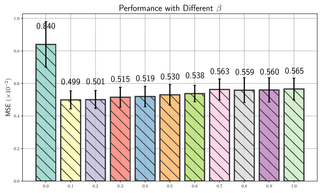
As Figure 10 shows, varying the value of $\beta$ gives different reconstruction performances with all the other settings kept the same. When $\beta=1.0$, the update to CNP $\theta$ is fully determined by the value of NCE. In fact, this corresponds to the lowest results among all different $\beta$ values. This may suggest the design choice of $\beta$ in practice.

We also find that $\beta=0.1$ works best for all the experiments involved in this work. Note that this combination is used only for updating CNP. As part of the iterative optimization, the EBM parameters $\varphi$ are solely optimized with respect to the NCE value.

Appendix H Computational Complexity Comparison.

In Section 5.3, we have discussed the complexity overhead on CNPs introduced by adversarial training, taking CNP for example, from $O(C+T)$ to $O(C+T+2T)$, where $C$ is the number context points and $T$ is the number of target points. The additional $2T$ account for the computation of EBM with $T$ true observations and $T$ CNP predictions.

We now include an empirical comparison between CNP and CNP-ADV with all the datasets studied in this paper. The comparison is based on elapsed time difference with one epoch. We perform the relative comparison, i.e., the elapsed time of CNP for each dataset is set to 1. Then we can compare how much longer it will take for CNP-ADV than for CNP.

The ratio of overhead elapsed time depends on the specific network design (i.e., encoder $h$, decoder $g$) of CNPs, as well as the size of dataset (i.e., the number of functions).

Figure 11: The comparison of relative elapsed time without/with adversarial training of running for 1 epoch.

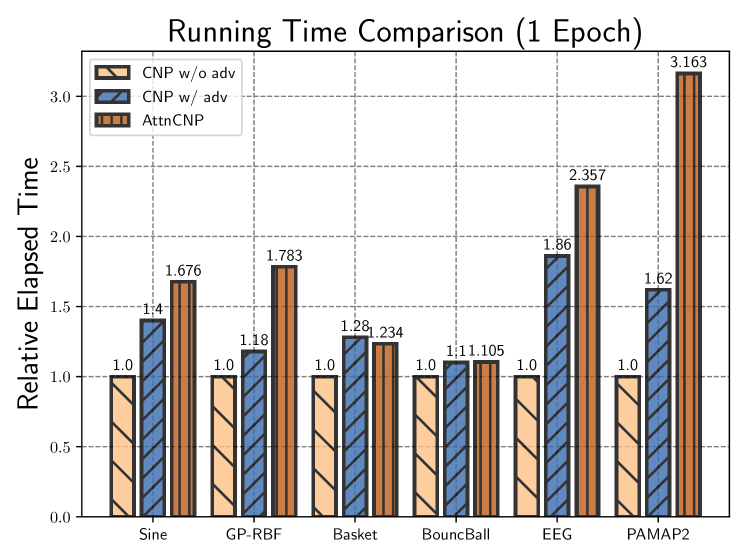
We also include the relative running time between CNP and AttentiveCNP (Kim et al., 2019) for a clearer comparison. The complexity of AttentiveCNP (ACNP) is of $O(C(C+T))$ because self-attention for every context and cross-attention for every target.

References

- Alemi et al. (2018) Alemi, A., Poole, B., Fischer, I., Dillon, J., Saurous, R. A., and Murphy, K. Fixing a broken elbo. In International Conference on Machine Learning, pp. 159–168. PMLR, 2018.
- Aneja et al. (2021) Aneja, J., Schwing, A., Kautz, J., and Vahdat, A. A contrastive learning approach for training variational autoencoder priors. Advances in neural information processing systems, 34:480–493, 2021.
- Bose et al. (2018) Bose, A. J., Ling, H., and Cao, Y. Adversarial contrastive estimation. arXiv preprint arXiv:1805.03642, 2018.
- Brown et al. (2020) Brown, T., Mann, B., Ryder, N., Subbiah, M., Kaplan, J. D., Dhariwal, P., Neelakantan, A., Shyam, P., Sastry, G., Askell, A., et al. Language models are few-shot learners. Advances in neural information processing systems, 33:1877–1901, 2020.
- Chehab et al. (2022) Chehab, O., Gramfort, A., and Hyvärinen, A. The optimal noise in noise-contrastive learning is not what you think. In Uncertainty in Artificial Intelligence, pp. 307–316. PMLR, 2022.
- Chen et al. (2020) Chen, T., Kornblith, S., Norouzi, M., and Hinton, G. A simple framework for contrastive learning of visual representations. In International conference on machine learning, pp. 1597–1607. PMLR, 2020.
- Du & Mordatch (2019) Du, Y. and Mordatch, I. Implicit generation and modeling with energy based models. Advances in Neural Information Processing Systems, 32, 2019.
- Foong et al. (2020) Foong, A., Bruinsma, W., Gordon, J., Dubois, Y., Requeima, J., and Turner, R. Meta-learning stationary stochastic process prediction with convolutional neural processes. In Larochelle, H., Ranzato, M., Hadsell, R., Balcan, M. F., and Lin, H. (eds.), Advances in Neural Information Processing Systems, volume 33, pp. 8284–8295. Curran Associates, Inc., 2020. URL https://proceedings.neurips.cc/paper/2020/file/5df0385cba256a135be596dbe28fa7aa-Paper.pdf.
- Gao et al. (2020) Gao, R., Nijkamp, E., Kingma, D. P., Xu, Z., Dai, A. M., and Wu, Y. N. Flow contrastive estimation of energy-based models. In Proceedings of the IEEE/CVF Conference on Computer Vision and Pattern Recognition, pp. 7518–7528, 2020.
- Garnelo et al. (2018a) Garnelo, M., Rosenbaum, D., Maddison, C., Ramalho, T., Saxton, D., Shanahan, M., Teh, Y. W., Rezende, D., and Eslami, S. A. Conditional neural processes. In International Conference on Machine Learning, pp. 1704–1713. PMLR, 2018a.
- Garnelo et al. (2018b) Garnelo, M., Schwarz, J., Rosenbaum, D., Viola, F., Rezende, D. J., Eslami, S. M. A., and Teh, Y. W. Neural processes, 2018b.
- Goldberger et al. (2000) Goldberger, A. L., Amaral, L. A., Glass, L., Hausdorff, J. M., Ivanov, P. C., Mark, R. G., Mietus, J. E., Moody, G. B., Peng, C.-K., and Stanley, H. E. Physiobank, physiotoolkit, and physionet: components of a new research resource for complex physiologic signals. circulation, 101(23):e215–e220, 2000.
- Gondal et al. (2021) Gondal, M. W., Joshi, S., Rahaman, N., Bauer, S., Wuthrich, M., and Schölkopf, B. Function contrastive learning of transferable meta-representations. In International Conference on Machine Learning, pp. 3755–3765. PMLR, 2021.
- Goodfellow et al. (2020) Goodfellow, I., Pouget-Abadie, J., Mirza, M., Xu, B., Warde-Farley, D., Ozair, S., Courville, A., and Bengio, Y. Generative adversarial networks. Communications of the ACM, 63(11):139–144, 2020.
- Gordon et al. (2020) Gordon, J., Bruinsma, W. P., Foong, A. Y. K., Requeima, J., Dubois, Y., and Turner, R. E. Convolutional conditional neural processes. In 8th International Conference on Learning Representations, ICLR 2020, Addis Ababa, Ethiopia, April 26-30, 2020. OpenReview.net, 2020. URL https://openreview.net/forum?id=Skey4eBYPS.
- Gui et al. (2021) Gui, J., Sun, Z., Wen, Y., Tao, D., and Ye, J. A review on generative adversarial networks: Algorithms, theory, and applications. IEEE Transactions on Knowledge and Data Engineering, 2021.
- Gutmann & Hyvärinen (2010) Gutmann, M. and Hyvärinen, A. Noise-contrastive estimation: A new estimation principle for unnormalized statistical models. In Proceedings of the thirteenth international conference on artificial intelligence and statistics, pp. 297–304. JMLR Workshop and Conference Proceedings, 2010.
- Gutmann & Hyvärinen (2012) Gutmann, M. U. and Hyvärinen, A. Noise-contrastive estimation of unnormalized statistical models, with applications to natural image statistics. Journal of machine learning research, 13(2), 2012.
- Holderrieth et al. (2021) Holderrieth, P., Hutchinson, M. J., and Teh, Y. W. Equivariant learning of stochastic fields: Gaussian processes and steerable conditional neural processes. In International Conference on Machine Learning, pp. 4297–4307. PMLR, 2021.
- Hospedales et al. (2021) Hospedales, T., Antoniou, A., Micaelli, P., and Storkey, A. Meta-learning in neural networks: A survey. IEEE transactions on pattern analysis and machine intelligence, 44(9):5149–5169, 2021.
- Kallidromitis et al. (2021) Kallidromitis, K., Gudovskiy, D., Kazuki, K., Iku, O., and Rigazio, L. Contrastive neural processes for self-supervised learning. In Asian Conference on Machine Learning, pp. 594–609. PMLR, 2021.
- Kim et al. (2021) Kim, D., Cho, S., Lee, W., and Hong, S. Multi-task processes. arXiv preprint arXiv:2110.14953, 2021.
- Kim et al. (2019) Kim, H., Mnih, A., Schwarz, J., Garnelo, M., Eslami, A., Rosenbaum, D., Vinyals, O., and Teh, Y. W. Attentive neural processes. In Proceedings of the International Conference on Learning Representations (ICLR), 2019.
- Kingma & Welling (2013) Kingma, D. P. and Welling, M. Auto-encoding variational bayes. arXiv preprint arXiv:1312.6114, 2013.
- Le et al. (2018) Le, T. A., Kim, H., Garnelo, M., Rosenbaum, D., Schwarz, J., and Teh, Y. W. Empirical evaluation of neural process objectives. In NeurIPS workshop on Bayesian Deep Learning, 2018.
- LeCun et al. (2006) LeCun, Y., Chopra, S., Hadsell, R., Ranzato, M., and Huang, F. A tutorial on energy-based learning. Predicting structured data, 1(0), 2006.
- Lucey et al. (2014) Lucey, P., Bialkowski, A., Carr, P., Yue, Y., and Matthews, I. How to get an open shot: Analyzing team movement in basketball using tracking data. In Proceedings of the 8th annual MIT SLOAN sports analytics conference, 2014.
- Ma & Collins (2018) Ma, Z. and Collins, M. Noise contrastive estimation and negative sampling for conditional models: Consistency and statistical efficiency. arXiv preprint arXiv:1809.01812, 2018.
- Markou et al. (2022) Markou, S., Requeima, J., Bruinsma, W. P., Vaughan, A., and Turner, R. E. Practical conditional neural processes via tractable dependent predictions. arXiv preprint arXiv:2203.08775, 2022.
- Mathieu et al. (2021) Mathieu, E., Foster, A., and Teh, Y. On contrastive representations of stochastic processes. Advances in Neural Information Processing Systems, 34:28823–28835, 2021.
- Mattei & Frellsen (2018) Mattei, P.-A. and Frellsen, J. Leveraging the exact likelihood of deep latent variable models. Advances in Neural Information Processing Systems, 31, 2018.
- Nguyen & Grover (2022) Nguyen, T. and Grover, A. Transformer neural processes: Uncertainty-aware meta learning via sequence modeling. In International Conference on Machine Learning, pp. 16569–16594. PMLR, 2022.
- Nijkamp et al. (2019) Nijkamp, E., Hill, M., Zhu, S.-C., and Wu, Y. N. Learning non-convergent non-persistent short-run mcmc toward energy-based model. Advances in Neural Information Processing Systems, 32, 2019.
- Norcliffe et al. (2021) Norcliffe, A., Bodnar, C., Day, B., Moss, J., and Liò, P. Neural ode processes. arXiv preprint arXiv:2103.12413, 2021.
- Øksendal (2003) Øksendal, B. Stochastic differential equations. In Stochastic differential equations, pp. 65–84. Springer, 2003.
- Oord et al. (2018) Oord, A. v. d., Li, Y., and Vinyals, O. Representation learning with contrastive predictive coding. arXiv preprint arXiv:1807.03748, 2018.
- Pang et al. (2020) Pang, B., Han, T., Nijkamp, E., Zhu, S.-C., and Wu, Y. N. Learning latent space energy-based prior model. Advances in Neural Information Processing Systems, 33:21994–22008, 2020.
- Radford et al. (2021) Radford, A., Kim, J. W., Hallacy, C., Ramesh, A., Goh, G., Agarwal, S., Sastry, G., Askell, A., Mishkin, P., Clark, J., et al. Learning transferable visual models from natural language supervision. In International Conference on Machine Learning, pp. 8748–8763. PMLR, 2021.
- Reiss & Stricker (2012) Reiss, A. and Stricker, D. Introducing a new benchmarked dataset for activity monitoring. In 2012 16th international symposium on wearable computers, pp. 108–109. IEEE, 2012.
- Rezende & Viola (2018) Rezende, D. J. and Viola, F. Taming vaes. arXiv preprint arXiv:1810.00597, 2018.
- Rybkin et al. (2021) Rybkin, O., Daniilidis, K., and Levine, S. Simple and effective vae training with calibrated decoders. In International Conference on Machine Learning, pp. 9179–9189. PMLR, 2021.
- Tieleman (2008) Tieleman, T. Training restricted boltzmann machines using approximations to the likelihood gradient. In Proceedings of the 25th international conference on Machine learning, pp. 1064–1071, 2008.
- Ton et al. (2021) Ton, J.-F., Lucian, C., Teh, Y. W., and Sejdinovic, D. Noise contrastive meta-learning for conditional density estimation using kernel mean embeddings. In International Conference on Artificial Intelligence and Statistics, pp. 1099–1107. PMLR, 2021.
- Uehara et al. (2018) Uehara, M., Matsuda, T., and Komaki, F. Analysis of noise contrastive estimation from the perspective of asymptotic variance. arXiv preprint arXiv:1808.07983, 2018.
- Vaswani et al. (2017) Vaswani, A., Shazeer, N., Parmar, N., Uszkoreit, J., Jones, L., Gomez, A. N., Kaiser, Ł., and Polosukhin, I. Attention is all you need. Advances in neural information processing systems, 30, 2017.
- Wang & Van Hoof (2020) Wang, Q. and Van Hoof, H. Doubly stochastic variational inference for neural processes with hierarchical latent variables. In International Conference on Machine Learning, pp. 10018–10028. PMLR, 2020.
- Wang & van Hoof (2022) Wang, Q. and van Hoof, H. Learning expressive meta-representations with mixture of expert neural processes. In Advances in neural information processing systems, 2022.
- Williams & Rasmussen (2006) Williams, C. K. and Rasmussen, C. E. Gaussian processes for machine learning, volume 2. MIT press Cambridge, MA, 2006.
- Xiao et al. (2020) Xiao, Z., Kreis, K., Kautz, J., and Vahdat, A. Vaebm: A symbiosis between variational autoencoders and energy-based models. arXiv preprint arXiv:2010.00654, 2020.
- Ye & Yao (2022) Ye, Z. and Yao, L. Contrastive conditional neural processes. In Proceedings of the IEEE/CVF Conference on Computer Vision and Pattern Recognition, pp. 9687–9696, 2022.
- Yildiz et al. (2019) Yildiz, C., Heinonen, M., and Lahdesmaki, H. Ode2vae: Deep generative second order odes with bayesian neural networks. Advances in Neural Information Processing Systems, 32, 2019.