Polyhedral Aspects of Feedback Vertex Set
and Pseudoforest Deletion Set

Abstract

We consider the feedback vertex set problem in undirected graphs (FVS). The input to FVS is an undirected graph $G=(V,E)$ with non-negative vertex costs. The goal is to find a least cost subset of vertices $S\subseteq V$ such that $G-S$ is acyclic. FVS is a well-known NP-hard problem with no $(2-\epsilon)$-approximation assuming the Unique Games Conjecture and it admits a $2$-approximation via combinatorial local-ratio methods [BBF95, BG96] which can also be interpreted as LP-based primal-dual algorithms [CGHW98]. Despite the existence of these algorithms for several decades, there is no known polynomial-time solvable LP relaxation for FVS with a provable integrality gap of at most $2$. More recent work [CM16] developed a polynomial-sized LP relaxation for a more general problem, namely Subset FVS, and showed that its integrality gap is at most $13$ for Subset FVS, and hence also for FVS.

Motivated by this gap in our knowledge, we undertake a polyhedral study of FVS and related problems. In this work, we formulate new integer linear programs (ILPs) for FVS whose LP-relaxation can be solved in polynomial time, and whose integrality gap is at most $2$. The new insights in this process also enable us to prove that the formulation in [CM16] has an integrality gap of at most $2$ for FVS. Our results for FVS are inspired by new formulations and polyhedral results for the closely-related pseudoforest deletion set problem (PFDS). Our formulations for PFDS are in turn inspired by a connecton to the densest subgraph problem. We also conjecture an extreme point property for a LP-relaxation for FVS, and give evidence for the conjecture via a corresponding result for PFDS.

1 Introduction

We consider the feedback vertex set problem in undirected graphs. For a graph $G=(V,E)$, a subset $U\subseteq V$ is a feedback vertex set if $G-U$ is acyclic; in other words $U$ is a hitting set for the cycles of $G$. In the feedback vertex set problem (FVS), the input is an undirected graph $G=(V,E)$ with non-negative vertex costs $c\mathrel{\mathop{\mathchar 58\relax}}V\rightarrow\R_{\geq 0}$ and the goal is to find a feedback vertex set of minimum cost, i.e., $\min\left\{\sum_{u\in U}c(u)\mathrel{\mathop{\mathchar 58\relax}}U\subseteq V\ \text{and $U$ is a feedback vertex set for $G$}\right\}$. FVS is a fundamental vertex deletion problem in the field of combinatorial optimization and appears in Karp’s list of 21 NP-Complete problems (as a decision version). We consider the approximability of FVS, in particular via polynomial-time solvable polyhedral formulations. First, we mention some known lower bounds. Via a simple reduction, the well-known weighted vertex cover problem can be reduced to FVS in an approximation preserving fashion. Hence, known results on vertex cover imply that there is no polynomial-time $(2-\epsilon)$-approximation for every fixed constant $\epsilon>0$ under the Unique Games Conjecture (UGC) [KR08] and that there is no polynomial-time $(1.36-\epsilon)$-approximation for every fixed constant $\epsilon>0$ under the $P\neq NP$ assumption [DS05].

Approximation algorithms for the unweighted version of FVS (UFVS), i.e., when all vertex costs are one, have been studied since 1980s. An $O(\log n)$-approximation for UFVS is implicit in the work of Erdös and Pósa [EP62]; Monien and Schulz [MS81] seem to be the first ones to explicitly study the problem, and obtained an $O(\sqrt{\log n})$-approximation for UFVS. Bar-Yehuda, Geiger, Naor, and Roth [BYGNR98] improved the ratio for UFVS to $4$, and also noted that an $O(\log n)$-approximation holds for FVS. Soon after that, Bafna, Berman, and Fujito [BBF95], and independently Becker and Geiger [BG96], obtained $2$-approximation algorithms for FVS. While [BBF95] explicitly uses the local-ratio terminology, [BG96] describes the algorithm in a purely combinatorial fashion. Although the algorithm in [BBF95] is described via the local-ratio method, the underlying LP relaxation is not obvious. As observed in [BYGNR98], the natural hitting set LP relaxation for FVS has an integrality gap of $\Theta(\log n)$. Chudak, Goemans, Hochbaum, and Williamson [CGHW98] described exponential sized integer linear programming (ILP) formulations for FVS, and showed that the algorithms in [BBF95, BG96] can be viewed as primal-dual algorithms with respect to the LP relaxations of these formulations. This also established that these LP relaxations have an integrality gap of at most $2$.

We recall the integer linear program (ILP) formulation and the associated LP-relaxation from [CGHW98]. For a graph $G=(V,E)$ and a subset $S\subseteq V$, let $E[S]\mathrel{\mathop{\mathchar 58\relax}}=\left\{\left\{u,v\right\}\in E\mathrel{\mathop{\mathchar 58\relax}}u,v\in S\right\}$ and $G[S]\mathrel{\mathop{\mathchar 58\relax}}=(S,E[S])$, and for a vertex $v\in V$, let $d_{S}(v)$ denote the degree of $v$ in $G[S]$. We will denote the following polyhedron as the strong density polyhedron and the constraints describing the polyhedron as strong density constraints:

$$P_{\text{SD}}(G) \mathrel{\mathop{\mathchar 58\relax}}=\left\{x\in\R^{V}_{\geq 0}\mathrel{\mathop{\mathchar 58\relax}}\ \sum\nolimits_{u\in S}(d_{S}(u)-1)x_{u}\geq|E[S]|-|S|+1\ \forall S\text{ such that }E[S]\not=\emptyset\right\}.$$ (1)

Chudak, Goemans, Hochbaum, and Williamson proved that strong density constraints are valid for FVS and that the following is an integer linear programming formulation for FVS:

$$\min\left\{\sum\nolimits_{u\in V}c_{u}x_{u}\mathrel{\mathop{\mathchar 58\relax}}\ x\in P_{\text{SD}}(G)\cap\Z^{V}\right\}.$$ (FVS-IP: SD)

They interpreted the local-ratio algorithm from [BBF95] as a primal-dual algorithm with respect to the LP-relaxation of (FVS-IP: SD) that we explicitly write below:

$$\min\left\{\sum\nolimits_{u\in V}c_{u}x_{u}\mathrel{\mathop{\mathchar 58\relax}}\ x\in P_{\text{SD}}(G)\right\}.$$ (FVS-LP: SD)

It is, however, not known whether (FVS-LP: SD) can be solved in polynomial time! Equivalently, it is open to design a polynomial-time separation oracle for the family of strong density constraints. Moreover, there has been no other polynomial-time solvable LP relaxation through which one could obtain a $2$-approximation for FVS. This status leads to the following natural question:

Question 1.

Does there exist an ILP formulation for FVS whose LP-relaxation can be solved in polynomial time and has an integrality gap at most $2$?

The lack of solvable LP relaxations for FVS has also been a stumbling block for the design of approximation algorithms for a generalization of FVS called the subset feedback vertex set problem (Subset-FVS) [ENSZ00]: the input is a weighted graph $G$ and a terminal set $T\subseteq V$, and the goal is to remove a minimum cost subset of vertices $S$ to ensure that $G-S$ has no cycle containing a terminal $t\in T$. There is an $8$-approximation for Subset-FVS [ENZ00] but it is quite complex. Motivated by these considerations, Chekuri and Madan [CM16] formulated a polynomial-sized integer linear program for Subset-FVS and showed that the integrality gap of its LP-relaxation is at most $13$. They explicitly raised the question of whether the integrality gap of their formulation is better for FVS; in fact it is open whether their formulation’s integrality gap is at most $2$ for Subset-FVS.

In this work, we provide an affirmative answer to Question 1 by undertaking a polyhedral study of FVS and a closely related problem, namely the pseudoforest deletion set problem that will be described shortly. In addition to formulating polynomial-time solvable LP relaxations with small integrality gap, it is also of interest to find algorithms that can round fractional solutions to the LP relaxations, and to understand properties of extreme points of the corresponding polyhedra. Based on several interrelated technical considerations, we conjecture the following property for the strong density polyhedron:

Conjecture 1.

Let $G=(V,E)$ be a graph that contains a cycle. For every extreme point $x$ of the polyhedron $P_{\text{SD}}(G)$, there exists a vertex $u\in V$ such that $x_{u}\geq 1/2$.

This conjecture would lead to an alternative proof that the integrality gap of the LP-relaxation (FVS-LP: SD) is at most $2$ via iterative rounding (instead of the primal-dual technique). Although we were unable to resolve this conjecture for the strong density polyhedron, we were able to show that a variant of the conjecture holds for a weak density polyhedron (to be defined later). The weak density polyhedron closely resembles the strong density polyhedron and is associated with an ILP formulation of the pseudoforest deletion set problem. We also discuss extreme point properties for other formulations later in the paper.

Pseudoforest Deletion Set Problem (PFDS).

A connected graph is a pseudotree if it has exactly one cycle; in other words there is an edge whose removal results in a spanning tree. A graph is a pseudoforest if each of its connected components is a pseudotree. For a graph $G=(V,E)$, a subset $U\subseteq V$ is a pseudoforest deletion set if $G-U$ is a pseudoforest. In the pseudoforest deletion set problem (PFDS), the input is an undirected graph $G=(V,E)$ with non-negative vertex costs $c\mathrel{\mathop{\mathchar 58\relax}}V\rightarrow\R_{\geq 0}$ and the goal is to find a pseudoforest deletion set of minimum cost, i.e., $\min\left\{\sum_{u\in U}c(u)\mathrel{\mathop{\mathchar 58\relax}}U\subseteq V\ \text{and $U$ is a pseudoforest deletion set for $G$}\right\}$. Intuitively one can see that PFDS is closely related to FVS. Note that any feasible solution for FVS in a given graph $G$ is a feasible solution to the PFDS instance on $G$. Also, finding an FVS in a graph that is a pseudoforest is easy: for each connected component that is a pseudotree, we remove the cheapest vertex in its unique cycle. PFDS and FVS are special cases of the more general $\ell$-pseudoforest deletion problem that was introduced in [PRS18] from the perspective of parameterized algorithms (FVS corresponds to $\ell=0$ and PFDS to $\ell=1$). Lin, Feng, Fu, and Wang [LFFW19] studied approximation algorithms for $\ell$-pseudoforest deletion problem. In this paper, we restrict attention to PFDS and FVS and do not discuss the more general problem. The status of PFDS is very similar to that of FVS. It has an approximation preserving reduction from the vertex cover problem and consequently, it is NP-hard, and does not have a polynomial time $(2-\epsilon)$-approximation for every constant $\epsilon>0$ assuming the UGC. It admits a polynomial-time $2$-approximation based on the local-ratio technique [LFFW19]. The authors in [LFFW19] do not discuss LP relaxations for PFDS. However, the local-ratio technique of [LFFW19] can be converted to an LP-based $2$-approximation for PFDS following the ideas in [CGHW98]. We describe the associated LP relaxation. A graph $G=(V,E)$ is a $2$-pseudotree if it is connected and has $|E|\geq|V|+1$ (i.e., the graph has at least $2$ edges in addition to a spanning tree). We will denote the following polyhedra as weak density polyhedron and $2$-pseudotree cover polyhedron respectively, and the constraints describing them as weak density constraints and $2$-pseudotree cover constraints respectively:

$$P_{\text{WD}}(G) \mathrel{\mathop{\mathchar 58\relax}}=\left\{x\in\R^{V}_{\geq 0}\mathrel{\mathop{\mathchar 58\relax}}\ \sum\nolimits_{u\in S}(d_{S}(u)-1)x_{u}\geq|E[S]|-|S|\ \forall S\subseteq V\right\},\text{ and}$$ (2)

$$P_{\text{2-PT-cover}}(G) \mathrel{\mathop{\mathchar 58\relax}}=\left\{x\in\R^{V}_{\geq 0}\mathrel{\mathop{\mathchar 58\relax}}\sum\nolimits_{u\in U}x_{u}\geq 1\ \forall U\subseteq V\text{ such that $G[U]$ is a $2$-pseudotree}\right\}.$$ (3)

We encourage the reader to compare and contrast the weak density constraints with the strong density constraints. Weak density constraints and $2$-pseudotree covering constraints are valid for PFDS. In particular, the following are ILP formulations for PFDS:

$$\min \left\{\sum\nolimits_{u\in V}c_{u}x_{u}\mathrel{\mathop{\mathchar 58\relax}}\ x\in P_{\text{WD}}(G)\cap\Z^{V}\right\}\text{ and}$$ (PFDS-IP: WD)

$$\min \left\{\sum\nolimits_{u\in V}c_{u}x_{u}\mathrel{\mathop{\mathchar 58\relax}}\ x\in P_{\text{WD}}(G)\cap P_{\text{2-PT-cover}}(G)\cap\Z^{V}\right\}.$$ (PFDS-IP: WD-and-2PT-cover)

The local-ratio technique for PFDS due to Lin, Feng, Fu, and Wang [LFFW19] can be converted to a $2$-approximation for PFDS with respect to the following LP-relaxation via the primal-dual technique:

$$\min\left\{\sum\nolimits_{u\in V}c_{u}x_{u}\mathrel{\mathop{\mathchar 58\relax}}\ x\in P_{\text{WD}}(G)\cap P_{\text{2-PT-cover}}(G)\right\}.$$ (PFDS-LP: WD-and-2PT-cover)

The family of $2$-pseudotree cover constraints admits a polynomial-time separation oracle (see Section 3.1). However, we do not know a polynomial-time separation oracle for the family of weak density constraints (similar to the status of strong density constraints), and for this reason we do not know how solve (PFDS-IP: WD-and-2PT-cover) in polynomial time. We emphasize that weak density constraints will play a crucial role in our polynomial-sized integer linear program for FVS with integrality gap at most $2$. Furthermore, we prove an extreme point property of the weak density polyhedron that closely resembles the extreme point property of the strong density polyhedron mentioned in 1.

1.1 Results

We recall that our main goal is to formulate an integer linear program (ILP) for FVS whose LP-relaxation has integrality gap at most $2$. As our first result, we show how to achieve this goal for PFDS by giving a new ILP formulation. We will subsequently use the properties of our new ILP formulation for PFDS to achieve the goal for FVS.

Our new ILP for PFDS is based on Charikar’s LP for the densest subgraph problem (DSG) [Cha00]. In DSG, the input is an undirected graph $G=(V,E)$ and the goal is to find an induced subgraph $G[S]$ of maximum density where the density of $S\subseteq V$ is defined as $\frac{|E(S)|}{|S|}$. We define the density of $G$ to be $\max\{|E[S]|/|S|\mathrel{\mathop{\mathchar 58\relax}}\emptyset\neq S\subseteq V\}$. We note that a graph is a pseudoforest if and only if its density is at most one. Thus, PFDS can equivalently be phrased as the problem of finding a minimum cost subset of vertices to delete so that the remaining graph has density at most one. Charikar formulated an LP to compute the density of a graph. The dual of Charikar’s LP can be interpreted as a fractional orientation problem. Using that dual, we obtain an ILP for PFDS. Our ILP for PFDS is based on the following polyhedron that will be denoted as the orientation polyhedron:

$$P_{\text{orient}}(G)\mathrel{\mathop{\mathchar 58\relax}}=\left\{(x,y)\mathrel{\mathop{\mathchar 58\relax}}\begin{array}[]{l}x_{u}+x_{v}+y_{e,u}+y_{e,v}\geq 1\ \forall e\in E\mathrel{\mathop{\mathchar 58\relax}}e=uv\\ x_{u}+\sum_{e\in\delta(u)}y_{e,u}\leq 1\ \forall u\in V\\ x_{u}\geq 0\ \forall u\in V\\ y_{e,u}\geq 0\ \forall e\in\delta(u),u\in V.\end{array}\right\}.$$

We will denote the projection of $P_{\text{orient}}(G)$ to the $x$ variables by $Q_{\text{orient}}(G)$.

Theorem 1.

The following are integer linear programming formulations for PFDS for a graph $G=(V,E)$ with non-negative costs $c\mathrel{\mathop{\mathchar 58\relax}}V\rightarrow\R_{\geq 0}$:

$$\min \left\{\sum\nolimits_{u\in V}c_{u}x_{u}\mathrel{\mathop{\mathchar 58\relax}}x\in Q_{\text{orient}}(G)\cap\Z^{V}\right\}\text{ and}$$ (PFDS-IP: orient)

$$\min \left\{\sum\nolimits_{u\in V}c_{u}x_{u}\mathrel{\mathop{\mathchar 58\relax}}x\in Q_{\text{orient}}(G)\cap P_{\text{2-PT-cover}}(G)\cap\Z^{V}\right\}.$$ (PFDS-IP: orient-and-2PT-cover)

Moreover, we have the following properties:

1. $Q_{\text{orient}}(G)\subseteq P_{\text{WD}}(G)$ for every graph $G$ and there exist graphs $G$ for which $Q_{\text{orient}}(G)\subsetneq P_{\text{WD}}(G)$.

2. The integrality gap of the following LP-relaxation is at most $2$:

   $$\min \left\{\sum\nolimits_{u\in V}c_{u}x_{u}\mathrel{\mathop{\mathchar 58\relax}}x\in Q_{\text{orient}}(G)\cap P_{\text{2-PT-cover}}(G)\right\}.$$ (PFDS-LP: orient-and-2PT-cover)

3. There exists a polynomial-time separation oracle for the family of $2$-pseudotree cover constraints.

We note that the upper bound of $2$ on the integrality gap of (PFDS-LP: orient-and-2PT-cover) mentioned in Theorem 1 is tight as shown in Figure 1. As a consequence of Theorem 1, we immediately obtain an integer linear program for PFDS whose LP-relaxation is solvable in polynomial time and has integrality gap at most $2$ — namely (PFDS-IP: orient-and-2PT-cover). We also bound the integrality gap of the LP-relaxation of (PFDS-IP: orient), but this will be based on extreme point properties and will be discussed later in this section.

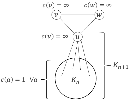
Figure 1: An example showing that the integrality gap of (PFDS-LP: orient-and-2PT-cover) tends to $2$ as $n$ tends to infinity. Consider the graph $G=(V,E)$ as shown above (where $K_{n}$ denotes the complete graph on $n$ vertices) with cost of every vertex $a\in V-\{u,v,w\}$ being $1$ and costs of vertices $u,v,w$ being infinite. The optimum value of (PFDS-IP: orient-and-2PT-cover) is $n-1$. The optimum value of (PFDS-LP: orient-and-2PT-cover) is at most $n/2$: the solution $x_{a}=1/2$ for every vertex $a\in V-\{u,v,w\}$, $x_{u}=x_{v}=x_{w}=0$, $y_{e,a}=0$ for all edges $e=ab$ where $a,b\in V-\{u,v,w\}$, $y_{uv,v}=y_{vw,w}=y_{wu,u}=1$, $y_{uv,u}=y_{vw,v}=y_{wu,w}=0$, and $y_{ua,a}=1/2$, $y_{ua,u}=0$ for every $a\in V-\{u,v,w\}$ is feasible for (PFDS-LP: orient-and-2PT-cover) and has cost $n/2$.

Next, we focus on formulating an ILP for FVS whose LP-relaxation has integrality gap at most $2$ and is polynomial-time solvable. In order to achieve this goal, we formulate an intermediate ILP for FVS whose LP-relaxation has integrality gap at most $2$, but it is unclear if this LP-relaxation is polynomial-time solvable. We will later formulate a polynomial-sized ILP for FVS whose LP-relaxation is at least as strong as that of the intermediate ILP, thereby achieving our goal.

Our intermediate ILP is based on weak density constraints and the following polyhedron that will be denoted as the cycle cover polyhedron:

$$P_{\text{cycle-cover}}(G) \mathrel{\mathop{\mathchar 58\relax}}=\left\{x\in\R^{V}_{\geq 0}\mathrel{\mathop{\mathchar 58\relax}}\sum\nolimits_{u\in U}x_{u}\geq 1\ \forall U\subseteq V\text{ such that $G[U]$ is a cycle}\right\}.$$ (4)

We will denote the constraints describing the cycle cover polyhedron as cycle cover constraints.

Theorem 2.

The following is an integer linear programming formulation for FVS for a graph $G=(V,E)$ with non-negative costs $c\mathrel{\mathop{\mathchar 58\relax}}V\rightarrow\R_{\geq 0}$:

$$\min\left\{\sum\nolimits_{u\in V}c_{u}x_{u}\mathrel{\mathop{\mathchar 58\relax}}x\in P_{\text{WD}}(G)\cap P_{\text{cycle-cover}}(G)\cap\Z^{V}\right\}.$$ (FVS-IP: WD-and-cycle-cover)

Moreover, we have the following properties:

1. The integrality gap of the following LP-relaxation is at most $2$:

   $$\min\left\{\sum\nolimits_{u\in V}c_{u}x_{u}\mathrel{\mathop{\mathchar 58\relax}}x\in P_{\text{WD}}(G)\cap P_{\text{cycle-cover}}(G)\right\}.$$ (FVS-LP: WD-and-cycle-Cover)

2. There exists a polynomial-sized formulation for $P_{\text{cycle-cover}}(G)$.

Theorem 2 shows that (FVS-IP: WD-and-cycle-cover) is an ILP for FVS whose LP-relaxation (FVS-LP: WD-and-cycle-Cover) has integrality gap at most $2$. However, we do not have a polynomial-time algorithm to solve the LP-relaxation (FVS-LP: WD-and-cycle-Cover) — this is because, we do not have a polynomial-time separation oracle for the family of weak density constraints (although we do have a polynomial-time separation oracle for the family of cycle cover constraints). We will use Theorem 1 in conjunction with Theorem 2 to prove the following result:

Theorem 3.

There exists a polynomial-sized integer linear programming formulation for FVS whose LP-relaxation has integrality gap at most $2$.

We prove Theorem 3 by showing three different polynomial-sized integer linear programs for FVS all of whose LP-relaxations have integrality gap at most $2$:

1. The first formulation is

   $$\min\left\{\sum\nolimits_{u\in V}c_{u}x_{u}\mathrel{\mathop{\mathchar 58\relax}}x\in Q_{\text{orient}}(G)\cap P_{\text{cycle-cover}}(G)\cap\Z^{V}\right\}.$$ (FVS-IP: orient-and-cycle-cover)

   By Theorem 1, we have that $Q_{\text{orient}}(G)\subseteq P_{\text{WD}}(G)$. As a consequence of Theorem 2, the integrality gap of the following LP-relaxation is also at most $2$:

   $$\min\left\{\sum\nolimits_{u\in V}c_{u}x_{u}\mathrel{\mathop{\mathchar 58\relax}}x\in Q_{\text{orient}}(G)\cap P_{\text{cycle-cover}}(G)\right\}.$$ (FVS-LP: orient-and-cycle-cover)

   Both $Q_{\text{orient}}(G)$ and $P_{\text{cycle-cover}}(G)$ admit a polynomial-sized description, and thus, we have a polynomial-sized ILP for FVS whose LP-relaxation has integrality gap at most $2$.

2. The second formulation is the Chekuri-Madan formulation who, as we remarked earlier, formulated an ILP for Subset-FVS and showed that the integrality gap of its LP-relaxation is at most $13$ [CM16]. We show that their LP-relaxation specialized for FVS has integrality gap at most $2$ by proving that it is at least as strong as (FVS-LP: orient-and-cycle-cover). Our result gives additional impetus to improving the integrality gap of the LP-relaxation for Subset-FVS.

3. Our third formulation to prove Theorem 3 is based on the orientation perspective, but without cycle cover constraints (as opposed to our first formulation). Here, we give an orientation based ILP formulation whose associated polyhedron is contained in the strong density polyhedron. Since the integrality gap of (FVS-LP: SD) is at most $2$ (as shown by Chudak, Goemans, Hochbaum, and Williamson [CGHW98]), the integrality gap of our third formulation is also at most $2$.

We emphasize that the proof of the integrality gap of the LP-relaxation of all three of our ILPs rely on the integrality gap bound of (FVS-LP: WD-and-cycle-Cover) or (FVS-LP: SD). It would be interesting to have a direct proof: in particular, it would be useful to design a primal rounding algorithm (for arbitrary LP-optimum solutions or for extreme point LP-optimum solutions) that yields a $2$-approximate solution.

Extreme point properties.

Motivated by 1 and the goal of designing primal rounding algorithms for the LP relaxations for FVS, we investigate extreme point properties of the weak density polyhedron and the orientation polyhedron. Although we were unable to resolve 1 for the strong density polyhedron, we were able to prove an extreme point property for the weak density polyhedron.

Theorem 4.

Let $G=(V,E)$ be a graph that is not a pseudoforest. For every extreme point $x$ of the polyhedron $P_{\text{WD}}(G)$, there exists a vertex $u\in V$ such that $x_{u}\geq 1/3$.

Our proof of Theorem 4 is based on a conditional supermodularity property—if all coordinates are small, then the weak density constraints have a supermodular property; we use this supermodular property to show the existence of a structured basis for the extreme point which is subsequently used to arrive at a contradiction. To the best of authors’ knowledge, the conditional supermodularity property based proof has not previously appeared in the literature on iterated rounding, and might be of independent interest. Theorem 4 leads to the following corollary.

Corollary 4.1.

The integrality gap of the following LP-relaxation of (PFDS-IP: WD) is at most $3$:

$$\min\left\{\sum\nolimits_{u\in V}c_{u}x_{u}\mathrel{\mathop{\mathchar 58\relax}}x\in P_{\text{WD}}(G)\right\}.$$ (PFDS-LP: WD)

4.1 can be seen to follow from Theorem 4 by the iterative rounding technique, where we repeatedly apply the following two steps until the graph $G$ is a pseudoforest: (1) Compute an extreme point optimum solution $x$ of (PFDS-LP: WD). (2) By Theorem 4, there exists a vertex $u\in V$ such that $x_{u}\geq 1/3$; include the vertex $u$ in the solution and remove it from the graph $G$. The approximation factor of the solution constructed by this procedure relative to the starting extreme point optimum solution to the LP is at most $3$.

The example given in Figure 2(a) shows that the $(1/3)$-bound in Theorem 4 and the integrality gap of $3$ mentioned in 4.1 are both tight.

(a) The unique extreme point in the weak density polyhedron along the all-ones objective direction for the butterfly graph is as shown. The largest coordinate is $1/3$ and all other coordinates are $0$. Consequently, the integrality gap of the LP $\min\{\sum_{u\in V}x_{u}\mathrel{\mathop{\mathchar 58\relax}}x\in P_{\text{WD}}(G)\}$ is at least $3$.

(b) A minimal extreme point in the orientation polyhedron along the all-ones objective direction for the butterfly graph is as shown. The largest $x$-coordinate is $1/3$ and all other $x$-coordinates are $0$. Consequently, the integrality gap of the LP $\min\{\sum_{u\in V}x_{u}\mathrel{\mathop{\mathchar 58\relax}}x\in P_{\text{orient}}(G)\}$ is at least $3$.

We emphasize that the extreme point result given in Theorem 4 and the integrality gap result mentioned in Corollary 4.1 are interesting only from a polyhedral viewpoint currently, and are not of help from the perspective of algorithm design. This is because, implementing the above-mentioned iterative rounding procedure requires us to solve the LP-relaxation (PFDS-LP: WD) in polynomial time, but we do not know how to do this yet.

We next show that although $Q_{\text{orient}}(G)$ is a subset of $P_{\text{WD}}(G)$ (as shown in Theorem 1), the extreme point result for $P_{\text{WD}}(G)$ given in Theorem 4 still holds for $Q_{\text{orient}}(G)$. We will say that an extreme point of a polyhedron is minimal if for each variable, reducing the value of that variable by any $\epsilon>0$ while keeping the rest of the variables unchanged results in a point that is outside the polyhedron. We note that extreme points of a polyhedron along non-negative objective directions will be minimal.

Theorem 5.

Let $G=(V,E)$ be a graph that is not a pseudoforest. For every minimal extreme point $(x,y)$ of the polyhedron $P_{\text{orient}}(G)$, there exists a vertex $u\in V$ such that $x_{u}\geq 1/3$.

Theorem 5 leads to the following corollary (similar to 4.1 that follows from Theorem 4):

Corollary 5.1.

The integrality gap of the following LP-relaxation of (PFDS-IP: orient) is at most $3$:

$$\min\left\{\sum\nolimits_{u\in V}c_{u}x_{u}\mathrel{\mathop{\mathchar 58\relax}}x\in Q_{\text{orient}}(G)\right\}$$ (PFDS-LP: orient)

Moreover, given an extreme point optimum solution $x$ for the LP, there exists a polynomial time algorithm to obtain an integral feasible solution $x^{\prime}$ for the LP-relaxation such that $\sum_{u\in V}c_{u}x^{\prime}_{u}\leq 3\sum_{u\in V}c_{u}x_{u}$.

5.1 can be seen to follow from Theorem 5 by the iterative rounding technique, where we repeatedly apply the following two steps until the graph $G$ is a pseudoforest: (1) Compute an extreme point optimum solution $x$ of $\min\left\{\sum_{u\in V}c_{u}x_{u}\mathrel{\mathop{\mathchar 58\relax}}x\in Q_{\text{orient}}(G)\right\}$. (2) By Theorem 5, there exists a vertex $u\in V$ such that $x_{u}\geq 1/3$; include the vertex $u$ in the solution and remove it from the graph $G$. The approximation factor of this procedure is $3$. In contrast to the weak density constraints based LP, namely (PFDS-LP: WD), we can solve the orientation based LP, namely (PFDS-LP: orient), in polynomial time.

The example given in Figure 2(b) shows that the $(1/3)$-factor in Theorem 5 and the integrality gap of $3$ mentioned in 5.1 are both tight.

Figure 3: The unique extreme point optimum for (FVS-LP: WD-and-cycle-Cover) along the all-ones objective direction on the complete graph $K_{4}$ is as shown. Consequently, the integrality gap of (FVS-LP: WD-and-cycle-Cover) is at least $3$.

Remark 1.

In the spirit of using iterative rounding to bound the integrality gap (e.g., Theorem 4 that leads to 4.1 and Theorem 5 that leads to 5.1), it is tempting to bound the integrality gap of (FVS-LP: WD-and-cycle-Cover) by proving an extreme point result. In particular, if we could show that every extreme point optimum of (FVS-LP: WD-and-cycle-Cover) had a coordinate with value at least $1/2$, then we would have an alternative proof of the integrality gap bound mentioned in Theorem 2 via the iterative rounding technique. However, the example given in Figure 3 shows that there exists an extreme point optimum of (FVS-LP: WD-and-cycle-Cover) all of whose coordinates have value at most $1/3$.

Organization.

In Section 3, we prove properties of the orientation polyhedron and show Theorem 1. In Section 4, we prove properties of the weak density polyhedron, show that the cycle cover polyhedron admits a polynomial-sized formulation, and show Theorem 2. In Section 5, we show three different polynomial-sized ILPs for FVS whose LP-relaxation has integrality gap at most $2$, thereby proving Theorem 3. In Sections 6 and 7, we prove extreme point properties of the weak density polyhedron and the orientation polyhedron and show Theorem 4 and Theorem 5 respectively.

2 Preliminaries

For a minimization IP $\min\{c^{T}x\mathrel{\mathop{\mathchar 58\relax}}Ax\leq b,x\in\Z^{n}_{\geq 0}\}$, the integrality gap of its LP-relaxation $\min\{c^{T}x\mathrel{\mathop{\mathchar 58\relax}}Ax\leq b,x\geq 0\}$ is the maximum ratio, over all non-negative cost functions, of the minimum cost of a feasible solution to the IP and that of the LP, i.e., $\max_{c\in\R^{n}}\min\{c^{T}x\mathrel{\mathop{\mathchar 58\relax}}Ax\leq b,x\in\Z^{n}_{\geq 0}\}/\min\{c^{T}x\mathrel{\mathop{\mathchar 58\relax}}Ax\leq b,x\geq 0\}$. For a graph $G=(V,E)$, we will use $\delta(A,B)$ to denote the set of edges with exactly one end-vertex in $A$ and exactly one end-vertex in $B$. We summarize the results of Lin, Feng, Fu, and Wang [LFFW19] in a manner that will be useful for our polyhedral study.

Theorem 6.

(PFDS-IP: WD) and (PFDS-IP: WD-and-2PT-cover) are ILP formulations for PFDS. Furthemore, the LP-relaxation (PFDS-LP: WD-and-2PT-cover) has integrality gap at most $2$.

We emphasize that Lin, Feng, Fu, and Wang did not prove Theorem 6 directly, but their local ratio based algorithm and standard techniques to convert local ratio based algorithms to LP-based primal-dual algorithms (following the ideas in [CGHW98]) lead to the theorem.

3 Polynomial-time solvable LP-relaxation for PFDS with integrality gap at most $2$

In this section, we restate and prove Theorem 1.

See 1

Proof.

In order to show that (PFDS-IP: orient) and (PFDS-IP: orient-and-2PT-cover) are ILP formulations for PFDS, it suffices to show that the ILP (PFDS-IP: orient) is a formulation for PFDS. This is because $2$-pseudotree cover constraints are valid for PFDS.

For a subgraph $\tilde{G}=(\tilde{V},\tilde{E})$ of the graph $G$, we let $d_{\tilde{G}}(u)\mathrel{\mathop{\mathchar 58\relax}}=|\delta(u)\cap\tilde{E}|$ denote the degree of the vertex $u$ in the subgraph $\tilde{G}$. We now define an intermediate polyhedron ${P}_{\text{WD-Subgraphs}}(G)$.

$${P}_{\text{WD-Subgraphs}}(G) \mathrel{\mathop{\mathchar 58\relax}}=\left\{x\in\R^{V}_{\geq 0}\mathrel{\mathop{\mathchar 58\relax}}\ \sum_{u\in\tilde{V}}(d_{\tilde{G}}(u)-1)x_{u}\geq|\tilde{E}|-|\tilde{V}|\ \forall\text{ subgraphs $\tilde{G}=(\tilde{V},\tilde{E})$ of $G$}.\right\}.$$ (5)

We note that ${P}_{\text{WD-Subgraphs}}(G)\subseteq P_{\text{WD}}(G)$. We will use the following claim to show that the ILP (PFDS-IP: orient) formulates PFDS and also to conclude that $Q_{\text{orient}}(G)\subseteq{P}_{\text{WD-Subgraphs}}(G)$.

Claim 1.

$Q_{\text{orient}}(G)\subseteq{P}_{\text{WD-Subgraphs}}(G)$.

Proof.

Let $x\in Q_{\text{orient}}(G)$. Then, there exists a vector $y$ such that $(x,y)\in P_{\text{orient}}(G)$. Let $\tilde{G}=(\tilde{V},\tilde{E})$ be an arbitrary subgraph of $G$. We have the following:

$$|\tilde{E}| \leq\sum_{e=vw\in\tilde{E}}(x_{v}+x_{w}+y_{e,v}+y_{e,w})$$

$$=\sum_{v\in\tilde{V}}(d_{\tilde{G}}(v)-1)x_{v}+\sum_{v\in\tilde{V}}\left(x_{v}+\sum_{e\in\delta_{\tilde{G}}(v)}y_{e,v}\right)$$

$$\leq\sum_{v\in\tilde{V}}(d_{\tilde{G}}(v)-1)x_{v}+|\tilde{V}|,$$

where the inequalities are because the vector $(x,y)\in P_{\text{orient}}$. Rearranging the above inequality gives the constraint for $\tilde{G}$ given in ${P}_{\text{WD-Subgraphs}}(G)$. Hence, $x\in{P}_{\text{WD-Subgraphs}}(G)$. ∎

1 can be strengthened to show that $Q_{\text{orient}}(G)={P}_{\text{WD-Subgraphs}}(G)$, but we will not need this stronger version for the purposes of this theorem.

We now show that the ILP (PFDS-IP: orient) formulates PFDS. Let $S\subseteq V$ be a pseudoforest deletion set, i.e., the subgraph $F\mathrel{\mathop{\mathchar 58\relax}}=G-S$ is a pseudoforest. Let $x\mathrel{\mathop{\mathchar 58\relax}}=\chi^{S}\in\{0,1\}^{V}$ denote the indicator vector of the set $S$. Select an arbitrary orientation of the pseudoforest $F$ such that the maximum indegree of every vertex is at most $1$, and let $y_{e,v}\mathrel{\mathop{\mathchar 58\relax}}=1$ for the edge $e=vw$ if $e$ is an edge of $F$ that is oriented towards $v$, and $y_{e,v}\mathrel{\mathop{\mathchar 58\relax}}=0$ otherwise. Then, $(x,y)\in P_{\text{orient}}(G)$.

Next, suppose $x\in Q_{\text{orient}}(G)\cap\Z^{V}$. Then, we have that $x\in\{0,1\}^{V}$. By 1, $x\in{P}_{\text{WD-Subgraphs}}(G)\subseteq P_{\text{WD}}(G)$. Since (PFDS-IP: WD) is an ILP formulation for PFDS by Theorem 6, it follows that the set $S\mathrel{\mathop{\mathchar 58\relax}}=\{u\in V\mathrel{\mathop{\mathchar 58\relax}}x_{u}=1\}$ is a pseudoforest deletion set for the graph $G$. This concludes the proof that the ILP (PFDS-IP: orient) formulates PFDS.

We now prove the additional three conclusions of the theorem statement.

1. By Claim 1, we have that $Q_{\text{orient}}(G)\subseteq{P}_{\text{WD-Subgraphs}}(G)\subseteq P_{\text{WD}}(G)$. We now show that there is a graph $G$ such that ${P}_{\text{WD-Subgraphs}}(G)\subsetneq P_{\text{WD}}(G)$. In particular, we consider the graph $K_{5}=(V,E)$ where $V=\{v_{1},v_{2},\ldots,v_{5}\}$ and $E={V\choose 2}$. Let $x=(7/12,7/12,1/12,0,0)$. We note that $x\in P_{\text{WD}}(K_{5})$. We now show that $x\not\in{P}_{\text{WD-Subgraphs}}(K_{5})$. Consider the subgraph $\tilde{G}=(\tilde{V},\tilde{E})$ obtained by removing the edge $\{v_{1},v_{2}\}$ from the graph $G$, i.e. $\tilde{V}=V$ and $\tilde{E}={V\choose 2}-\{v_{1},v_{2}\}$. Then, we have the following:

   $$\sum_{u\in\tilde{V}}(d_{\tilde{G}}(u)-1)x_{u}=3x_{1}+3x_{2}+4x_{3}+4x_{4}+4x_{5}=\frac{46}{12}<4=|\tilde{E}|-|\tilde{V}|.$$

   In particular, the vector $x$ does not satisfy the constraint of ${P}_{\text{WD-Subgraphs}}(K_{5})$ defined by the subgraph $\tilde{G}$. Thus, we have that $Q_{\text{orient}}(K_{5})\subseteq{P}_{\text{WD-Subgraphs}}(K_{5})\subset P_{\text{WD}}(K_{5})$.

2. By Theorem 6, the ILP (PFDS-IP: WD-and-2PT-cover) is a valid formulation of PFDS and its LP-relaxation (PFDS-LP: WD-and-2PT-cover) has integrality gap at most $2$. We have already shown that the ILP (PFDS-IP: orient-and-2PT-cover) is a valid formulation of PFDS and that $Q_{\text{orient}}(G)\subseteq P_{\text{WD}}(G)$. Consequently, the integrality gap of (PFDS-LP: orient-and-2PT-cover) is at most $2$.

3. The third conclusion follows from Section 3.1 in the next subsection. It is based on the fact that node-weighted Steiner tree for constant number of terminals is solvable in polynomial time. We present its proof in a separate subsection for clarity.

∎

3.1 Separation oracle for the family of $2$-pseudotree cover constraints

In this section, we show that the family of $2$-pseudotree cover constraints admits a polynomial time separation oracle.

lemmaNWtwoPTPolytime The family of $2$-pseudotree cover constraints admits a polynomial time separation oracle.

In order to solve the separation problem, it suffices to design a polynomial time algorithm for the Minimum Cost $2$-Pseudotree problem: The input to MC2PT is a vertex-weighted graph $\left(G=\left(V,E\right),w\mathrel{\mathop{\mathchar 58\relax}}V\rightarrow\R_{\geq 0}\right)$, and the goal is to compute a minimum weight subset $U\subseteq V$ of vertices such that $G[U]$ is a $2$-pseudotree, i.e.,

$$\min\left\{\sum\nolimits_{u\in U}w(u)\mathrel{\mathop{\mathchar 58\relax}}U\subseteq V\text{ and }G[U]\text{ is a }2\text{-pseudotree}\right\}.$$

Our strategy to solve MC2PT is to reduce it to solving a polynomial number of special instances of the Minimum Node-Weighted Steiner Tree (NWST), and use the result of [BWB18] which says that these special instances of NWST can be solved in polynomial time. Formally, the input to NWST is a vertex-weighted graph $\left(G=\left(V,E\right),w\mathrel{\mathop{\mathchar 58\relax}}V\rightarrow\R_{\geq 0}\right)$ and a terminal set $S\subseteq V$. We will say that a graph $H$ is a Steiner tree in $G$ for terminal set $S$ if $H$ is connected, acyclic, and is a subgraph of $G$ with $S\subseteq V_{H}$. Moreover, the weight of a subgraph $H$ of $G$ is the sum of weights of vertices in $H$. The NWST problem is to find a minimum weight Steiner tree in $G$ for terminal set $S$, i.e., $\min\{\sum_{u\in V_{H}}w(u)\mathrel{\mathop{\mathchar 58\relax}}H=(V_{H},E_{H})\text{ is a Steiner tree in }G\text{ for terminal set }S\}$. NWST can be solved in polynomial time if the number of terminals is a constant.

Proposition 1 (Theorem 1 of [BWB18]).

There exists a $O(3^{k}n+2^{k}n^{2}+n^{3})$ time algorithm for NWST, where $k$ denotes the number of terminals and $n$ denotes the number of vertices in the input instance.

The following proposition shows a correspondence between minimum weight $2$-pseudotrees in a vertex-weighted graph and Steiner trees.

Proposition 2.

Let $G=(V,E)$ be a graph with non-negative vertex weights $w\mathrel{\mathop{\mathchar 58\relax}}V\rightarrow\R_{\geq 0}$ and let $W\geq 0$. Then, there exists a subset $U\subseteq V$ such that $G[U]$ is a $2$-pseudotree with $\sum_{u\in U}w(u)\leq W$ if and only if there exists a pair of edges $e_{1}=u_{1}v_{1},e_{2}=u_{2}v_{2}$ in $G$ such that there exists a Steiner tree $H=(V_{H},E_{H})$ in the graph $G^{\prime}\mathrel{\mathop{\mathchar 58\relax}}=G-\{e_{1},e_{2}\}$ for terminal set $S\mathrel{\mathop{\mathchar 58\relax}}=\{u_{1},v_{1},u_{2},v_{2}\}$ with $\sum_{u\in V_{H}}w(u)\leq W$.

Proof.

We will say that a graph $T=(V_{T},E_{T})$ is a minimal $2$-pseudotree if it is connected and has exactly $|V_{T}|+1$ edges. Equivalently, $T$ has exactly $2$ edges in addition to a spanning tree. We observe that for a subset $U\subseteq V$, the subgraph $G[U]$ is a $2$-pseudotree if and only if there exists a subgraph $T=(U,E_{T})$ of $G[U]$ such that $T$ is a minimal $2$-pseudotree. Hence, it suffices to show that there exists a subset $U\subseteq V$ such that $G[U]$ has a subgraph that is a minimal $2$-pseudotree with $\sum_{u\in U}w(u)\leq W$ if and only if there exists a pair of edges $e_{1}=u_{1}v_{1},e_{2}=u_{2}v_{2}$ in $G$ such that there exists a Steiner tree $H=(V_{H},E_{H})$ in the graph $G^{\prime}\mathrel{\mathop{\mathchar 58\relax}}=G-\{e_{1},e_{2}\}$ for terminal set $S\mathrel{\mathop{\mathchar 58\relax}}=\{u_{1},v_{1},u_{2},v_{2}\}$ with $\sum_{u\in V_{H}}w(u)\leq W$. We prove this statement now.

Let $U\subseteq V$ such that $G[U]$ contains a subgraph $T=(U,E_{T})$ that is a minimal $2$-pseudotree with $\sum_{u\in U}w(u)\leq W$. Then, there exists a pair of edges $e_{1}=u_{1}v_{2}$ and $e_{2}=u_{2}v_{2}$ in $T$ such that the subgraph $H\mathrel{\mathop{\mathchar 58\relax}}=T-\{e_{1},e_{2}\}$ is acyclic, connected, and is a subgraph of $T$. In particular, we have that $H$ is acyclic, connected, and is a subgraph of $G^{\prime}\mathrel{\mathop{\mathchar 58\relax}}=G-\{e_{1},e_{2}\}$ with $S=\{u_{1},v_{1},u_{2},v_{2}\}\subseteq U=V(H)$. Hence, for the pair of edges $e_{1},e_{2}$ in $G$, we have that $H$ is a Steiner tree in $G^{\prime}$ for terminal set $S$ with $\sum_{u\in V(H)}w(u)=\sum_{u\in U}w(u)\leq W$.

Next, let $e_{1}=u_{1}v_{2},e_{2}=u_{2}v_{2}$ be a pair of edges in $G$ such that there exists a Steiner tree $H=(V_{H},E_{H})$ in the graph $G^{\prime}\mathrel{\mathop{\mathchar 58\relax}}=G-\{e_{1},e_{2}\}$ for terminal set $S=\{u_{1},v_{1},u_{2},v_{2}\}$ with $\sum_{u\in V_{H}}w(u)\leq W$. Consider the graph $T\mathrel{\mathop{\mathchar 58\relax}}=H+\{e_{1},e_{2}\}$. Then, $T$ is a minimal $2$-pseudotree. The vertex set of $T$ is $U\mathrel{\mathop{\mathchar 58\relax}}=V_{H}$ and $T$ is a subgraph of $G[U]$. Hence, we have a subset $U\subseteq V$ such that $G[U]$ has a subgraph that is a minimal $2$-pseudotree with $\sum_{u\in U}w(u)\leq W$. ∎

We now restate and prove Section 3.1.

Proof.

It suffices to show that MC2PT can be solved in polynomial time. Let $G=(V,E)$ with vertex weights $w\mathrel{\mathop{\mathchar 58\relax}}V\rightarrow\R_{\geq 0}$ be the input instance of MC2PT. Consider the following algorithm: for all pairs of edges $e_{1}=u_{1}v_{1}$ and $e_{2}=u_{2}v_{2}$ in $E$, use the algorithm guaranteed by Proposition 1 to solve NWST on the graph $G-\{e_{1},e_{2}\}$ with vertex weights $w$ for terminal set $\{u_{1},v_{1},u_{2},v_{2}\}$, and return the minimum weight solution over all instances. The correctness of the algorithm follows from Proposition 2. We now analyze the runtime of the algorithm. There are $O(|V|^{2})$ pairs of edges to enumerate. Furthermore, for each pair of edges, the associated NWST instance can be solved in polynomial time using the algorithm from Proposition 1 since each such instance has only four terminals. Thus, the algorithm runs in polynomial time. ∎

4 Weak Density and Cycle Cover Constraints for FVS

In this section, we prove Theorem 2. Let $G=(V,E)$ be the input graph with non-negative vertex costs $c\mathrel{\mathop{\mathchar 58\relax}}V\rightarrow\R_{\geq 0}$. By definition, the ILP $\min\{\sum_{u\in V}c_{u}x_{u}\mathrel{\mathop{\mathchar 58\relax}}x\in P_{\text{cycle-cover}}(G)\cap\Z^{V}\}$ formulates FVS. We note that weak density constraints are valid for FVS. Consequently, (FVS-IP: WD-and-cycle-cover) is an ILP formulation for FVS. The additional conclusions of Theorem 2 follow from Lemma 1 shown in Section 4.1 and Lemma 6 shown in Section 4.2.

4.1 Integrality gap of weak density and cycle cover constraints

In this section, we show that the integrality gap of (FVS-LP: WD-and-cycle-Cover) is at most $2$.

Lemma 1.

The integrality gap of the LP (FVS-LP: WD-and-cycle-Cover) is at most $2$.

Let $\calC$ be the set of cycles in the input graph $G$. Let $b(S)\mathrel{\mathop{\mathchar 58\relax}}=|E[S]|-|S|$ for all $S\subseteq V$. We rewrite (FVS-LP: WD-and-cycle-Cover) and its dual in Figure 4.

$\begin{array}[]{ll@{}ll}&\text{{Primal}:}&&\\ &&&\\ \text{min}&\displaystyle\sum\limits_{u\in V}c_{u}x_{u}&&\\ &&&\\ \text{s.t.}&\displaystyle\sum\limits_{u\in S}(d_{S}(u)-1)x_{u}\geq b(S),&&\forall S\subseteq V\\ &\displaystyle\sum\limits_{u\in C}x_{u}\geq 1&&\forall C\in\calC\\ &x_{u}\geq 0&&\forall u\in V\end{array}$ $\begin{array}[]{ll@{}ll}&\text{{Dual}:}&&\\ &&&\\ \text{max}&\displaystyle\sum\limits_{S\subseteq V}b(S)y_{S}+\displaystyle\sum\limits_{C\in\calC}z_{C}&&\\ &&&\\ \text{s.t.}&\displaystyle\sum\limits_{S\subseteq V\mathrel{\mathop{\mathchar 58\relax}}u\in S}(d_{S}(u)-1)y_{S}+\displaystyle\sum\limits_{C\in\calC\mathrel{\mathop{\mathchar 58\relax}}u\in C}z_{C}\leq w_{u}&&\forall u\in V\\ &y_{S}\geq 0&&\forall S\subseteq V\\ &z_{C}\geq 0&&\forall C\in\calC\end{array}$

Figure 4: WD-CC Primal and Dual LPs for FVS

We will need the definition of semi-disjoint cycles from [CGHW98]: A cycle $C$ in graph G is semi-disjoint (with respect to the graph $G$) if there is at most one vertex in $C$ of degree strictly larger than $2$. We call such a vertex as the pivot vertex of the semi-disjoint cycle. We note that such cycles can be viewed as “hanging off” the graph via their pivots which are cut vertices.

4.1.1 Minimal FVS and Weak Density Constraints

In this section, we show an important property of inclusion-wise minimal feedback vertex sets. Let $F$ be a feedback vertex set for a graph $G$. A witness cycle for a vertex $f\in F$ is a cycle $C$ of the graph $G$ such that $F\cap C=\{f\}$ i.e. $f$ is the only vertex that witnesses the cycle $C$. We note that every vertex of a minimal FVS must have a witness cycle. In Lemma 2, we show that for a graph with non-trivial degree and no semi-disjoint cycles, every minimal feedback vertex set is essentially a $2$-approximation to the optimal feedback vertex set with respect to an appropriate cost function. We note that our proof of the lemma appears implicitly in [CGHW98]. However, we include it here for completeness.

Lemma 2.

Let $G$ be a graph with minimum-degree at least $2$ and containing no semi-disjoint cycles. Then, for every minimal feedback vertex set $F$, we have that

$$\sum_{v\in F}(d(v)-1)\leq 2b(V).$$

Proof.

We first show a convenient sufficient condition that proves the claimed upper bound. We subsequently prove this sufficient condition by an edge-counting argument. Let $t$ denote the number of connected components in $G-F$.

Claim 2.

If $|\delta(F,V-F)|\geq|F|+2t$, then $\sum_{v\in F}(d(v)-1)\leq 2b(V)$.

Proof.

We have the following:

$$2|V|-|F| \leq|\delta(F,V-F)|+2(|V|-|F|-t)$$

$$=|\delta(F,V-F)|+2|E[V-F]|$$

$$=\sum_{v\in V-F}d(v)$$

$$=2|E|-\sum_{v\in F}d(v).$$

The above chain of inequalities gives us the claim (by rearranging terms). Here, the first inequality holds due to the hypothesis that $|\delta(F,V-F)|\geq|F|+2t$. The first equality holds because $G-F$ is acyclic. The final equality holds because the sum of all vertex degrees is $2|E|$. ∎

We now show that a minimal feedback vertex set $F$ has at least $|F|+2t$ edges crossing it. For this, we consider the auxiliary bipartite graph $H=(K\cup F,E_{H})$ as follows: Each vertex $k\in K$ corresponds to a connected component $C_{k}$ in $G-F$. For vertices $k\in K,f\in F$, the graph $H$ contains the edge $(k,f)$ if there exists a vertex $v\in C_{k}$ such that the edge $(v,f)\in E$ exists in the original graph $G$. Furthermore, we define the weight of an edge $(k,f)\in E_{H}$ as $w_{H}(k,f)\mathrel{\mathop{\mathchar 58\relax}}=|\delta_{G}(C_{k},f)|$. We note that $|K|=t$.

Since $F$ is an inclusionwise minimal feedback vertex set, every vertex $f\in F$ has a witness cycle. We note that there are no edges between the components of $G-F$. Thus, every witness cycle is completely contained in some component $C_{k}$ for some $k\in K$. In particular, this implies that in the graph $H$, every vertex $f\in F$ has an edge of weight at least $2$ incident on it. For each $f\in F$ pick an arbitrary such edge $e_{f}\in\delta_{H}(f)$ and call it $f$’s primary edge. Then, reducing the weight of all primary edges by $1$ still leaves all edges in $E_{H}$ with positive weight, but counts $|F|$ edges in the cut $|\delta(F,V-F)|$ in the original graph $G$. Let $H^{\prime}$ denote the residual graph after this weight reduction. By 2, it now suffices to show that the weight of all edges in $H^{\prime}$ is at least $2|K|$.

For this, we claim that each vertex $k\in K$ must have a cumulative edge-weight of at least $2$ incident on it in the residual graph $H^{\prime}$. By way of contradiction, suppose that there exists a vertex $k\in K$ with total incident edge-weight at most $1$. We consider two cases. First, suppose that $k$ has no incident edges. We recall that we reduced the weight of only primary edges in our weight-reduction step. Thus, if there was a primary edge incident to $k$, then $k$ would have a weight $1$ edge incident on it in the residual graph, contradicting the case assumption. Thus, there are no edges incident to $C_{k}$ in $G$, i.e. $C_{k}$ is a disconnected acyclic component of $G$. In particular, $C_{k}$ contains a leaf vertex, contradicting the hypothesis that the minimum degree of $G$ is at least $2$.

Next, consider the case where $k$ has a total weight of $1$ incident on it in the residual graph $H^{\prime}$. Let $f\in F$ be its unique neighbor in the residual graph. Then, $f$ must also be its unique neighbor in $H$. We note that if $C_{k}$ has only one edge to $f$ in $G$, then $C_{k}$ must contain a leaf node in $G$ as it is acyclic, a contradiction. Thus, $C_{k}$ does not contain any leaf nodes, is acyclic, and has exactly $2$ edges to $f$ in $G$. In particular, $C_{k}\cup\{f\}$ is a semi-disjoint cycle in $G$, contradicting the hypothesis that $G$ has no semi-disjoint cycles. ∎

4.1.2 Proof of Integrality Gap

In this section, we prove Lemma 1, i.e., we show that the integrality gap of the LP-relaxation for FVS given in Figure 4 is at most $2$. We prove this by constructing a dual feasible solution $(\overline{y},\overline{z})$ and a FVS $F$ such that the cost of $F$ is at most twice the dual objective value of $(\overline{y},\overline{z})$. This implies that the integrality gap of the LP is at most $2$ since the LP is a relaxation for FVS. We construct such a pair of solutions via a primal-dual algorithm. Our primal-dual algorithm is an extension of the $2$-approximation primal-dual algorithm due to [CGHW98]. We state our algorithm in Algorithm 1.

Algorithm 1 Primal-Dual for FVS

Input: (1) Graph $G=(V,E)$; (2) Vertex weights $w\mathrel{\mathop{\mathchar 58\relax}}V\rightarrow\mathbb{R_{+}}$.
Output: Feedback vertex set $F\subseteq V$.

1. Initialize $(y,z)\mathrel{\mathop{\mathchar 58\relax}}=0$, $i\mathrel{\mathop{\mathchar 58\relax}}=1$, $F\mathrel{\mathop{\mathchar 58\relax}}=\emptyset$, and $G_{1}=G$.

2. While the graph $G_{i}=(V_{i},E_{i})$ has a cycle:

   1. Recursively remove vertices of degree $1$ from $G_{i}$.

   2. If $G_{i}$ has a semi-disjoint cycle $C_{i}$: Define the set $S_{i}=C_{i}$ as the semi-disjoint cycle.

   3. Else: Define the set $S_{i}=V_{i}$ as the entire vertex set.

   4. Increase dual variable $y_{S_{i}}$ until the first dual constraint becomes tight for some vertex $u_{i}\in S_{i}$.

   5. Update $F\mathrel{\mathop{\mathchar 58\relax}}=F\cup\{u_{i}\}$
      $G_{i+1}\mathrel{\mathop{\mathchar 58\relax}}=G_{i}-u_{i}$
      $i\mathrel{\mathop{\mathchar 58\relax}}=i+1$.

3. Perform reverse-delete on $F$.

4. Return $F$.

Algorithm 1 is a primal-dual algorithm based on the LP relaxation for FVS given in Figure 4. The algorithm initializes with the dual feasible solution $(\overline{y}=0,\overline{z}=0)$. In the $i$th iteration of the while-loop, the algorithm selects a specific set $S_{i}$ of vertices (which is either a cycle $C_{i}$ or entire vertex set $V_{i}$) and increases the corresponding dual variable until a dual constraint for some vertex $v_{i}\in S_{i}$ becomes tight. It then includes the vertex $v_{i}$ into the FVS and removes $v_{i}$ from the graph. Adding $v_{i}$ to the candidate set $F$ is interpreted as setting the primal variable $x_{v_{i}}=1$. Thus, Algorithm 1 always maintains dual feasibility and primal complementary slackness (i.e., $x_{v_{i}}=1$ only if the dual constraint for $v_{i}$ is tight).

We now explain the reverse-delete procedure mentioned in Algorithm 1. Let $\ell$ be the number of iteration of the while loop. The reverse-delete procedure iteratively considers vertices in the reverse-order in which they were added into $F$, i.e. $v_{\ell},v_{\ell-1},\ldots v_{1}$. For every vertex in this order, the procedure checks whether removal of this vertex from $F$ is still a feasible FVS for $G$. If so, then the vertex is removed from $F$. We will later rely on reverse-delete to show that $F\cap S_{i}$ is a minimal FVS is $G[S_{i}]$ for every iteration $i$.

We now observe that the algorithm terminates in polynomial time to return a feasible FVS.

Lemma 3 (Feasibility and Runtime).

Algorithm 1 returns a feasible FVS for the input graph $G$ in polynomial time.

Proof.

Each step of the while loop and reverse-delete procedure can be implemented to run in polynomial time. In $i$th iteration of the while-loop, at least one vertex of the graph $G_{i}$ is removed. The empty graph has no cycles and so the while-loop will terminate in at most linear number of iterations. Furthermore, the reverse delete step considers every vertex in $F$ exactly once, and so, it also terminates in at most linear number of steps. The output set $F$ is a feasible FVS by the terminating condition of the while-loop and the fact that reverse-delete deletes a vertex only if its deletion maintains feasibility. ∎

We now bound the approximation factor of the solution $F$ returned by Algorithm 1. Let $(\overline{y},\overline{z})$ be the dual solution constructed by Algorithm 1 and let $\chi^{F}\in\{0,1\}^{V}$ be the indicator vector of $F$. We note that Lemma 3 implies that $\chi^{F}$ is a feasible solution to the primal LP. Let $\mathtt{primal}(\chi^{F}),\mathtt{dual}(\overline{y},\overline{z})$ denote the objective values of the primal and dual LPs for solutions $\chi^{F}$ and $(\overline{y},\overline{z})$ respectively.

Let $I_{1}\subseteq[\ell]$ denote the set of iterations in which the dual variable for the entire residual graph was increased (i.e. statement (b) of Algorithm 1 is executed) and let $I_{2}\subseteq[\ell]$ denote the set of iterations in which the dual variable for a semi-disjoint cycle in the residual graph was increased (i.e. statement (c) of Algorithm 1 is executed). For notational convenience, we let $F_{j}=F\cap\{v_{j}\}$ and $F_{\geq j}=\cup_{k\in[j,\ell]}F_{j}$. The next lemma shows that the set $S_{i}\cap F_{\geq i}$ is a minimal feedback vertex set for the subgraph $G[S_{i}]$ for each $i\in[\ell]$.

Lemma 4.

The set $S_{i}\cap F_{\geq i}$ is a minimal feedback vertex set for the subgraph $G[S_{i}]$ for each $i\in[\ell]$.

Proof.

We prove by induction on $\ell-i$. For the base case, we consider $i=\ell$. We observe that $F_{\geq\ell}=\{v_{\ell}\}$ as otherwise, the following two observations result in a contradiction: (i) The reverse-delete step only removes $v_{\ell}$ from $F$ if the set $F-\{v_{\ell}\}$ is a feasible feedback vertex set for $G$; and (ii) if $F-\{v_{\ell}\}$ were a FVS for $G$, then the algorithm would have terminated after the $(\ell-1)^{th}$ iteration. We note that $F_{\ell}$ is a FVS for $G_{\ell}$ as there was no $(\ell+1)^{th}$ iteration. If the set $S_{\ell}=V_{\ell}$ is the entire vertex set of the graph $G_{\ell}$, then $v_{\ell}\in V_{\ell}$. Alternatively, if the set $S_{\ell}$ is a semi-disjoint cycle $C_{\ell}$, then $v_{\ell}\in C_{\ell}$, as otherwise the cycle $C_{\ell}$ would remain in $G_{\ell+1}$ contradicting that there were only $\ell$ iterations. In both scenarios, the set $S_{\ell}\cap F_{\geq\ell}$ is a minimal FVS for $G[S_{\ell}]$.

For the inductive case, assume that $0\leq i<\ell$. By the inductive hypothesis, we have that the set $S_{j}\cap F_{\geq j}$ is a minimal FVS for the graph $G[S_{j}]$ for all $\ell\geq j>i$. We consider two cases based on whether the set $S_{i}$ is a semi-disjoint cycle of $G_{i}$ or the entire vertex set of $G_{i}$.

First, we consider the case where $S_{i}$ is a semi-disjoint cycle $C_{i}$. We need to show that $|F\cap C_{i}|=1$. We observe that $1\leq|F_{\geq i}|\leq 2$: The lower bound follows from the fact that the set $F_{\geq i}$ is a feasible FVS for $G_{i}$ and thus intersects all cycles in at least one vertex. The upper bound holds by the following three observations: (i) The vertex $v_{i}$ is the first vertex of the set $C_{i}$ to be selected into $F$ by the algorithm; (ii) If the vertex $v_{i}$ is the pivot vertex, then all vertices in $C_{i}-\{v_{i}\}$ get recursively removed and thus cannot be selected into $F$ in any subsequent iteration after $i$; and (iii) If the vertex $v_{i}$ is not the pivot vertex, then all vertices in $C_{i}-\{v_{i}\}$ except the pivot vertex get recursively removed due to step (a) and thus, only the pivot vertex can be included into $F$ in some subsequent iteration after $i$. We note that if scenario (ii) happens, then $F_{\geq i}\cap C_{i}=\{v_{i}\}$ and hence, $|F\cap C_{i}|=1$. Alternatively, suppose that scenario (iii) happens. If the pivot is never selected into $F$, then once again we have $F_{\geq i}\cap C_{i}=\{v_{i}\}$ and hence, $|F\cap C_{i}|=1$. Otherwise the pivot is selected into $F$ and the reverse-delete step processes the pivot vertex before processing $v_{i}$. If the reverse-delete step removes the pivot vertex from $F$, then once again we have $F_{\geq i}\cap C_{i}=\{v_{i}\}$ and hence, $|F\cap C_{i}|=1$. Otherwise, the reverse-delete step does not remove the pivot from $F$. Consider the iteration of reverse-delete that processes $v_{i}$—we need to show that reverse-delete will indeed remove $v_{i}$ in this iteration. We observe that the set $\{v_{k}\mathrel{\mathop{\mathchar 58\relax}}k\in[1,i-1]\}$ has not been processed by reverse-delete and this set intersects every cycle that is not entirely contained in $G_{i}$ (this is true since $G_{i}$ is the residual graph after removal of $\{v_{1},\ldots v_{i-1}\}$ along with recursively removing degree-1 vertices in each step). Since the pivot for $C_{i}$ is already in $F$ and the cycle $C_{i}$ is semi-disjoint in $G_{i}$, the reverse-delete step must remove the vertex $v_{i}$ from $F$ as $v_{i}$ intersects no cycles other than those already intersected by $F-\{v_{i}\}$. In particular, $F_{\geq i}\cap C_{i}$ is a singleton set consisting of the pivot vertex for $C_{i}$. Thus, in all cases we have that $|F_{\geq i}\cap C_{i}|=1$. It follows that $F_{i}$ is a minimal FVS for the cycle $G[C_{i}]$.

Next, we consider the case when $S_{i}=V_{i}$ is the entire vertex set of the subgraph $G_{i}$. Here, we consider the set of all cycles that $v_{i}$ intersects in $G$ and partition them into two types: (1) Cycles completely contained in $G_{i}$; and (2) cycles that include at least one vertex from $V-V_{i}$. Since $F_{\geq i}$ is a feasible FVS for $G_{i}$, we have that $F_{\geq i}$ intersects all cycles of the first type. Furthermore, since the vertices in $V-V_{i}$ do not exist in $G_{i}$, the set $\{v_{1},\ldots,v_{i-1}\}$ intersect all cycles of the second type. We recall that the set $F_{\geq i+1}$ is a minimal FVS for $G_{i+1}$.

We consider the first subcase where the set $F_{\geq i+1}$ is an FVS for the graph $G_{i}$. Then, the set $F_{\geq i+1}$ intersects all cycles contained in $G_{i}$. In particular, it intersects all cycles of type (1). Thus, the set $\{v_{1},\ldots,v_{i-1}\}\cup F_{\geq i+1}$ is a feasible FVS for the original graph $G$. Due to this, the reverse-delete step removes the vertex $v_{i}$ from $F$ and we have that $F_{\geq i}=F_{\geq i+1}$. Furthermore, by the inductive hypothesis we have that $F_{\geq i+1}$ is a minimal FVS for $G_{i+1}$. Thus, the set $F_{i}$ is a minimal FVS for $G_{i}=G[S_{i}]$.

We next consider the remaining subcase where the set $F_{\geq i+1}$ is not a FVS for the graph $G_{i}$. In particular, there must be a cycle of the first type that $v_{i}$ intersects, but none of the vertices of $F_{\geq i+1}$ intersect. In particular, the set $\{v_{1},\ldots,v_{i-1}\}\cup F_{\geq i+1}$ is a not feasible FVS for the original graph $G$ as the set does not intersect all type (1) cycles. Thus, the reverse-delete step cannot remove $v_{i}$ from $F$. By the induction hypothesis, we have that $F_{\geq i+1}$ is a minimal FVS for $G_{\geq i+1}$. Consequently, none of these vertices can be removed from $F_{\geq i}$ as the resulting set would not be a feasible FVS. It follows that $F_{\geq i}$ is a minimal FVS for $G_{i}=G[S_{i}]$. ∎

We show in Lemma 5 that the solution $F$ constructed by the algorithm has cost at most twice the objective value of the dual feasible solution $(\overline{y},\overline{z})$ constructed by the algorithm. We recall that $\chi^{F}\in\{0,1\}^{V}$ is the indicator vector of the set $F$ and $\mathtt{primal}(\chi^{F}),\mathtt{dual}(\overline{y},\overline{z})$ denote the objective values of the primal and dual LPs for solutions $\chi^{F}$ and $(\overline{y},\overline{z})$ respectively.

Lemma 5 (Integrality gap bound).

We have that

$$\mathtt{primal}(\chi^{F})\leq 2\cdot\mathtt{dual}(\overline{y},\overline{z}).$$

Proof.

We have that

$$\mathtt{primal}(\chi^{F}) =\sum_{v\in F}c_{v}$$

$$=\sum_{v\in F}\left(\sum_{S\subseteq V\mathrel{\mathop{\mathchar 58\relax}}v\in S}(d_{S}(v)-1)\overline{y}_{S}+\sum_{C\in\calC\mathrel{\mathop{\mathchar 58\relax}}v\in C}\overline{z}_{C}\right)$$

$$=\sum_{S\subseteq V}\overline{y}_{S}\sum_{v\in F\cap S}(d_{S}(v)-1)+\sum_{C\in\calC}\overline{z}_{C}\sum_{v\in F\cap C}1$$

$$=\sum_{i\in I_{1}}\overline{y}_{S_{i}}\sum_{v\in F\cap S_{i}}(d_{S_{i}}(v)-1)+\sum_{i\in I_{2}}\overline{z}_{C_{i}}|F\cap C_{i}|$$

$$\leq 2\sum_{i\in I_{1}}\overline{y}_{S_{i}}b(S_{i})+\sum_{i\in I_{2}}\overline{z}_{C_{i}}$$

$$\leq 2\cdot\mathtt{dual}(\overline{y},\overline{z}).$$

Here, the second equality follows by the primal complementary slackness maintained by Algorithm 1. The fourth equality follows by the fact that all dual variables that were not incremented during some iteration of Algorithm 1 have value zero. The first inequality follows by Lemma 4 and Lemma 2. ∎

Lemma 5 completes the proof of Lemma 1 since $\mathtt{dual}(\overline{y},\overline{z})\leq\mathtt{primal}(\chi^{F})$ by weak duality and the fact that the ILP $\min\{\sum_{u\in V}c_{u}x_{u}\mathrel{\mathop{\mathchar 58\relax}}x\in P_{\text{WD}}(G)\cap P_{\text{cycle-cover}}(G)\cap\Z^{V}\}$ is an ILP formulation for FVS (whose LP-relaxation is given in Figure 4). It also proves that the approximation factor of the solution $F$ returned by Algorithm 1 is at most $2$.

4.2 Polynomial-sized formulation of $P_{\text{cycle-cover}}(G)$

In this section, we show that $P_{\text{cycle-cover}}(G)$ can be expressed using polynomial number of variables and constraints. This is folklore, but we include its proof for the sake of completeness.

Lemma 6.

Let $G=(V,E)$ and $E^{\prime}\mathrel{\mathop{\mathchar 58\relax}}=\{e\in E\mathrel{\mathop{\mathchar 58\relax}}\ \exists\text{ cycle in $G$ containing }e\}$. The cycle cover polyhedron $P_{\text{cycle-cover}}(G)$ is the projection of the following polyhedron to $x$ variables:

$$P_{\text{dist-cycle-cover}}(G)\mathrel{\mathop{\mathchar 58\relax}}=\left\{(x,d)\in\R^{V}_{\geq 0}\times\R^{V\times E^{\prime}}_{\geq 0}\mathrel{\mathop{\mathchar 58\relax}}\ \begin{array}[]{l}{d_{s}^{e}=0}\hfill{\qquad\forall e=st\in E^{\prime}}\\ {d_{t}^{e}+x_{s}\geq 1}\hfill\qquad\forall e=st\in E^{\prime}\\ {d_{a}^{e}+x_{b}\geq d_{b}^{e}}\hfill\qquad\forall ab\in E,\ e\in E^{\prime}\end{array}\right\},$$ (6)

Consequently, $P_{\text{cycle-cover}}(G)$ admits a polynomial-sized description.

Proof.

Let $Q_{\text{dist-cycle-cover}}(G)$ be the projection of $P_{\text{dist-cycle-cover}}(G)$ to the $x$ variables. We prove that $Q_{\text{dist-cycle-cover}}(G)=P_{\text{cycle-cover}}(G)$.

We first show that $Q_{\text{dist-cycle-cover}}(G)\subseteq P_{\text{cycle-cover}}(G)$. Let $x\in Q_{\text{dist-cycle-cover}}(G)$. Let $d\in\R^{V\times E^{\prime}}_{\geq 0}$ be a vector such that $(x,d)\in P_{\text{dist-cycle-cover}}(G)$. It suffices to show that for every cycle $C$ in $G$, we have that $\sum_{u\in V(C)}x_{u}\geq 1$. Let $C$ be a cycle in $G$. Fix $e=st\in E(C)$. Then, $e\in E^{\prime}$ and hence, $d^{e}_{s}=0$, and $d^{e}_{t}+x_{s}\geq 1$. Let $a_{1}=s,a_{2},a_{3},\ldots,a_{r-1},a_{r}=t$ be the vertices of the cycle in that order. Then, we have the constraint $d^{e}_{a_{i}}+x_{a_{i+1}}\geq d^{e}_{a_{i+1}}$ for every $i\in[r-1]$. Adding these constraints gives us that $\sum_{i=2}^{r}x_{a_{i}}\geq d^{e}_{a_{r}}=d^{e}_{t}\geq 1-x_{s}=1-x_{a_{1}}$. Thus, the constraint $\sum_{i=1}^{r}x_{a_{i}}\geq 1$ holds.

Next, we show that $Q_{\text{dist-cycle-cover}}(G)\supseteq P_{\text{cycle-cover}}(G)$. Let $x\in P_{\text{cycle-cover}}(G)$. Let $d\in\R^{V\times E^{\prime}}_{\geq 0}$ be defined as follows: for each $e=st\in E^{\prime}$, let

$$d^{e}_{u}\mathrel{\mathop{\mathchar 58\relax}}=\min\left\{\sum_{v\in P-\{s\}}x_{v}\mathrel{\mathop{\mathchar 58\relax}}\ P\text{ is a path from $s$ to $u$ and $P\neq\{s,t\}$}\right\}.$$

We show that $(x,d)\in P_{\text{dist-cycle-cover}}(G)$. The vector $(x,d)$ is non-negative by definition. Let $e=st\in E^{\prime}$. Then, $d^{e}_{s}=0$ by definition. Moreover, $d^{e}_{t}+x_{s}\geq 1$ due to the following reasoning: let $P$ be a path from $s$ to $t$ such that $d^{e}_{t}=\sum_{v\in P-\{s\}}x_{v}$ and $P\neq\{s,t\}$. Then, $P$ concatenated with the edge $st$ forms a cycle $C$ and $d^{e}_{t}+x_{s}=x_{s}+\sum_{v\in P-\{s\}}x_{v}=\sum_{u\in V(C)}x_{u}\geq 1$. Finally, $d^{e}_{a}+x_{b}\geq d^{e}_{b}$ for every edge $ab\in E$ due to the following reasoning: for an edge $ab\in E$, let $P$ be a path from $s$ to $a$ such that $d^{e}_{a}=\sum_{v\in P-\{s\}}x_{v}$. Then, $P$ concatenated with $b$ is a path from $s$ to $b$ and consequently, $d^{e}_{b}\leq\sum_{v\in P+\{b\}-\{s\}}x_{v}$ by definition. ∎

5 Polynomial-sized LP-relaxations for FVS with integrality gap at most $2$

In this section, we prove Theorem 3 by giving three polynomial-sized LP-relaxations for FVS with integrality gap at most $2$. Our first formulation is based on orientation and cycle cover polyhedra and we show that its LP-relaxation is at least as strong as (FVS-LP: WD-and-cycle-Cover). Our second formulation is Chekuri-Madan’s formulation specialized for FVS and we show that its LP-relaxation is at least as strong as our first formulation. The strength of these formulations along with Theorem 2 imply that the integrality gap of the LP-relaxation of these two formulations is at most $2$. Our third formulation is based only on orientation constraints (without relying on cycle cover constraints). We show that its LP-relaxation is at least as strong as that of the strong density constraints based formulation. Since we know that the LP-relaxation of the strong density constraints based formulation has integrality gap at most $2$ (as shown by [CGHW98]), the integrality gap of the LP-relaxation of our third formulation is also at most $2$.

5.1 Orientation and Cycle Cover based Formulation

In this section, we give a polynomial-sized ILP for FVS based on orientation and cycle cover constraints. Moreover, we show that the integrality gap of the LP-relaxation of this formulation is at most $2$. Our ILP is based on the following lemma.

Lemma 7.

The following is an integer linear programming formulation for FVS for a graph $G=(V,E)$ with non-negative vertex costs $c\mathrel{\mathop{\mathchar 58\relax}}V\rightarrow\R_{\geq 0}$:

$$\min\left\{\sum_{u\in V}c_{u}x_{u}\mathrel{\mathop{\mathchar 58\relax}}x\in Q_{\text{orient}}(G)\cap P_{\text{cycle-cover}}(G)\cap\Z^{V}\right\}.$$

Moreover, its LP-relaxation has integrality gap at most $2$.

Proof.

The indicator vector $x$ of a feedback vertex set of $G$ is contained in $Q_{\text{orient}}(G)\cap P_{\text{cycle-cover}}(G)$. Moreover, every integral solution $x\in Q_{\text{orient}}(G)\cap P_{\text{cycle-cover}}(G)$ is the indicator vector of a feedback vertex set: since $x\in Q_{\text{orient}}(G)\cap\Z^{V}$, we have that $x\in\{0,1\}^{V}$ and since $x\in P_{\text{cycle-cover}}(G)$, we have that $x$ is the indicator vector of a feedback vertex.

We now show that the integrality gap of the LP-relaxation is at most $2$. By Lemma 1, $Q_{\text{orient}}(G)\subseteq P_{\text{WD}}(G)$ and hence, the integrality gap of the LP-relaxation is at most the integrality gap of (FVS-LP: WD-and-cycle-Cover). By Theorem 2, the integrality gap of (FVS-LP: WD-and-cycle-Cover) is at most $2$. ∎

Theorem 3 follows from Lemma 7 and Lemma 6 and by observing that $Q_{\text{orient}}(G)$ can be expressed using polynomial number of variables and constraints (see the description of $P_{\text{orient}}(G)$).

5.2 Chekuri-Madan’s Formulation

In this section, we show that the polynomial-sized ILP for FVS given by Chekuri and Madan is such that its LP-relaxation has integrality gap at most $2$. Chekuri and Madan formulated a polynomial-sized ILP for the more general problem of Subset Feedback Vertex Set (SFVS). SFVS is defined as follows: The input is a graph $G=(V,E)$ with non-negative vertex costs $c\mathrel{\mathop{\mathchar 58\relax}}V\rightarrow\R_{\geq 0}$ along with a set of terminals $T\subseteq V$. A subset $U$ of non-terminals is said to be a subset feedback vertex set if $G-U$ has no cycle containing a vertex of $T$. The goal is to find a least cost subset feedback vertex set. We will discuss Chekuri-Madan’s ILP for SFVS with some background and notation in Section 5.2.1, specialize it to FVS in Section 5.2.2, and show that the integrality gap of its LP-relaxation is at most $2$ in Section 5.2.3.

5.2.1 Chekuri-Madan’s ILP for SFVS

In this section, we discuss Chekuri-Madan’s ILP for SFVS. Let $H=(V_{H},E_{H})$ denote the input graph, $S_{H}\subseteq V_{H}$ denote the terminal set, and $c_{H}\mathrel{\mathop{\mathchar 58\relax}}V_{H}\rightarrow\mathbb{R}_{\geq 0}$ denote the vertex cost function. We will say that a cycle is interesting if it contains a terminal. Let $\calC_{H}$ denote the set of interesting cycles in the graph $H$.

Henceforth, we will assume that a SFVS of finite cost exists in the graph $H$. Furthermore, we will assume without loss of generality that the instance $H$ satisfies the following properties (see [CM16] for a justification of these assumptions):

1. the graph $H$ is connected,

2. each terminal $s_{i}\in S_{H}$ has infinite cost, is a degree two vertex with neighbors $a_{i},b_{i}$ having infinite cost,

3. no two terminals are connected by an edge or share a neighbor,

4. there exists a special non-terminal degree one vertex $r\in V$ with infinite cost, and

5. each interesting cycle contains at least two terminals.

Notation.

Throughout this section we will use the following notation: We let $k=|S_{H}|$ denote the number of terminals. We refer to the set $P_{i}\mathrel{\mathop{\mathchar 58\relax}}=\{a_{i},b_{i}\}$ as the pivot set for the terminal $s_{i}$, and the set $P_{H}=\cup_{i\in[k]}P_{i}$ as the set of all pivots. We define the set

$$\ell_{H}(u)=\{i\in[k]\mathrel{\mathop{\mathchar 58\relax}}\text{$s_{i}$ is reachable from $u$ via a path not containing any other terminals}\}\cup\{k+1\}$$

as the set of labels for each vertex $u\in V_{H}\backslash S$. We denote $\tilde{V}_{H}$ as the set of vertices in $V_{H}$ that are not in $S_{H}\uplus P_{H}\uplus\{r\}$. We denote $\tilde{E}_{H}$ as the set of edges in $E_{H}$ that are not incident to any terminals and the set $E^{\prime}_{H}$ as the set of edges incident to terminals. We will refer to $E^{\prime}_{H}$ as special edges.

Chekuri-Madan’s ILP.

See Figure 5 for Chekuri-Madan’s labelling-based ILP for SFVS. In this ILP, we have vertex variables $x_{u}$ for each $u\in\tilde{V}$ indicating whether the vertex $u$ is in the SFVS $F$, and vertex labelling variables $z_{u,i}$ for each $u\in\tilde{V}\cup P_{H},i\in[k]$ indicating whether vertex $u$ receives label $i$. We note that Figure 5 simplifies the exposition of the ILP from [CM16] by explicitly substituting the values for variables whose values are directly set by constraints, i.e. $x_{u}=0$ for $u\in S\cup\{r\}$, $z_{s_{i},i}=1$ for $i\in[k]$, and $z_{r,k+1}=1$. Moreover, it slightly strengthens the first constraint (Chekuri-Madan used a slightly weaker constraint: $x_{u}+\sum_{i\in[k+1]}z_{u,i}=1$).

The constraints can be interpreted as follows: Let $F$ be a minimal finite cost subset feedback vertex set of $H$. Constraint (1) says that if a vertex $u\in\tilde{V}_{H}$ is not in $F$, then it must receive exactly one of the labels in $\ell_{H}(u)$. Constraint (2) says that exactly one of $a_{i}$ and $b_{i}$ can receive the label $i$ for each $i\in[k]$. Constraint (3) is a spreading constraint that says that both end vertices of every non-special edge in $H-F$ must receive the same label. Constraint (4) is a cycle covering constraint and says that the solution $F$ must intersect every interesting cycle in at least one vertex. Constraint (5) ensures that the set $F$ contains no pivot vertices.

We now briefly address why a labeling satisfying the LP constraints must exist for every minimal finite weight subset feedback vertex set $F$ (see [CM16] for further details). We note that none of the vertices of $S\cup P\cup\{r\}$ are in $F$ as these have infinite cost. Let the graph $H^{\prime}=(V_{H^{\prime}},E_{H^{\prime}})$ be defined as $H^{\prime}=H-F$. For simplicity, we first assume that the graph $H^{\prime}$ is connected and then address the more general case when $H^{\prime}$ is not connected. Since there is no cycle containing any terminal in $H^{\prime}$, each terminal is a cut vertex in $H^{\prime}$. Consider the block-cut-vertex tree decomposition $T^{\prime}$ of $H^{\prime}$ — (refer to [Wes00] for details on block-cut-vertex tree decompositions). We label a vertex $u$ of $H^{\prime}$ as $i\in[k]$ if terminal $s_{i}$ is the first terminal encountered on any path from vertex $u$ to the root $r$ in the graph $H^{\prime}$. If no terminals are encountered, then we label the vertex as $k+1$. We note that such a labelling is well-defined as $T^{\prime}$ is the block-cut-vertex tree and the set $S$ are cut vertices. In this labelling, we observe that every non-special edge $uv\in\tilde{E}_{H^{\prime}}$ has the property that both end points receive the same label. Finally, in the case where $H^{\prime}$ is not connected, we can justify the existence of such a labeling by picking an arbitrary non-terminal vertex from each component, imagining a dummy edge connecting it to the root $r$, and considering the labeling corresponding to block-cut-vertex tree of this (implicit) graph.

Subset Feedback Vertex Set: min $\displaystyle\displaystyle\sum\limits_{u\in\tilde{V}_{H}}c_{u}x_{u}$ s.t. $\displaystyle(1)\ \$ $\displaystyle x_{u}+\sum_{i\in\ell_{H}(u)}z_{u,i}=1$ $\displaystyle\forall\ u\in\tilde{V}_{H}\cup P_{H}$ $\displaystyle(2)\ \$ $\displaystyle z_{a_{i},i}+z_{b_{i},i}=1$ $\displaystyle\forall\ i\in[k]$ $\displaystyle(3)\ \$ $\displaystyle x_{u}+z_{u,i}-z_{v,i}\geq 0$ $\displaystyle\forall\ uv\in\tilde{E}_{H},\ i\in[k+1]$ $\displaystyle(4)\ \$ $\displaystyle\sum_{u\in C}x_{u}\geq 1$ $\displaystyle\forall\ C\in\calC_{H}$ $\displaystyle(5)\ \$ $\displaystyle x_{u}=0$ $\displaystyle\forall\ u\in P_{H}$ $\displaystyle(6)\ \$ $\displaystyle z_{u,i}\geq 0$ $\displaystyle\forall\ \text{ $u\in\tilde{V}_{H}\cup P_{H},i\in[k+1]$}$ $\displaystyle(7)\ \$ $\displaystyle x_{u}\geq 0$ $\displaystyle\forall\ u\in\tilde{V}_{H}$ $\displaystyle(8)\ \$ $\displaystyle z_{u,i}\in\Z$ $\displaystyle\forall\ \text{ $u\in\tilde{V}_{H}\cup P_{H},i\in[k+1]$}$ $\displaystyle(9)\ \$ $\displaystyle x_{u}\in\Z$ $\displaystyle\forall\ u\in\tilde{V}_{H}$

Figure 5: Chekuri-Madan’s ILP for SFVS

5.2.2 Reduction from FVS to SFVS satisfying the Chekuri-Madan properties

FVS can be seen as a special case of SFVS where every vertex in the graph is a terminal. However, this simple reduction does not result in an SFVS instance satisfying the properties assumed by the Chekuri-Madan LP (see properties (i)–(v) mentioned in the first paragraph of Section 5.2.1). In this section, we show how to construct an SFVS instance from an FVS instance such that the SFVS instance satisfies the required properties. Let $G=(V_{G},E_{G})$ with vertex costs $c_{G}\mathrel{\mathop{\mathchar 58\relax}}V_{G}\rightarrow\R_{\geq 0}$ be the FVS instance. We will construct an SFVS instance $H=(V_{H},E_{H})$ with terminals $S_{H}$ and vertex costs $c_{H}\mathrel{\mathop{\mathchar 58\relax}}V_{H}\rightarrow\mathbb{R}_{\geq 0}$ satisfying the required properties. We may assume that the FVS instance $G$ has an infinite-weighted degree-1 root vertex $r$, satisfying property (iv) since adding such a vertex does not change the set of minimal feasible solutions. We construct $H$ as follows:

1. For each edge $e=uv\in E_{G}$, we subdivide the edge $e$ so that the edge becomes a path $u,a_{e},s_{e},b_{e},v$ of length $4$.

2. We let $S_{H}=\bigcup_{e\in E(G)}\{s_{e}\}$ denote the terminal set. Thus, the set $P_{e}\mathrel{\mathop{\mathchar 58\relax}}=\{a_{e},b_{e}\}$ is the set of pivot vertices for each terminal $s_{e}\in S_{H}$, and the set $P_{H}\mathrel{\mathop{\mathchar 58\relax}}=\bigcup_{e\in E(G)}P_{e}$ is the set of all pivots of the graph $H$.

3. We define the cost function as $c_{H}(u)=c_{G}(u)$ if $u\in V_{G}$, and $c_{H}(u)=\infty$ otherwise (i.e., if $u\in S_{H}\cup P_{H}$).

We observe that the graph $H$ satisfies properties (i)-(v) assumed by the Chekuri-Madan LP. The next proposition says that solving FVS in the graph $G$ with cost function $c_{G}$ is equivalent to solving SFVS in the graph $H$ with terminal set $S_{H}$ with cost function $c_{H}$. The proposition follows by construction.

Proposition 3.

Let $F\subseteq V_{G}$. The set $F$ is a feedback vertex set for $G$ if and only if the set $F$ is a subset feedback vertex set for the graph $H$ with terminal set $S_{H}$. Furthermore, the cost of $F$ in both graphs is the same, i.e. $c_{G}(F)=c_{H}(F)$.

Chekuri and Madan showed that the LP-relaxation of their ILP for SFVS given in Figure 6 has integrality gap at most $13$. It immediately follows that the integrality gap of that LP-relaxation on the instance $H$ constructed as above is also at most $13$. In the subsequent section, we tighten this integrality gap to $2$ for instances $H$ constructed as above.

5.2.3 Bounding the Integrality Gap

In this section, we show that the LP-relaxation of the ILP for SFVS given in Figure 5 for the instance $H$ constructed as given in the reduction in Section 5.2.2 has integrality gap at most $2$. We prove this by showing that the LP constraints imply orientation and cycle cover constraints. Consequently, the integrality gap of the LP-relaxation is at most that of $\min\{\sum_{u\in V}c_{u}x_{u}\mathrel{\mathop{\mathchar 58\relax}}x\in Q_{\text{orient}}(G)\cap P_{\text{cycle-cover}}(G)\}$. By Lemma 7, it follows that the integrality gap of the LP-relaxation is at most $2$.

We begin by simplifying the ILP given in Figure 5 for SFVS instances $H$ that are constructed from FVS instances as given in the reduction in Section 5.2.2. We make two observations that will help us in the simplification. The first observation is that each edge $e\in E_{G}$ corresponds to a unique terminal $s_{e}\in V_{H}$. Thus, we may replace the set $[k]$ which indexed the set of terminals in the LP of Figure 5 with the set $E_{G}$. For ease of exposition, we denote $e_{r}$ by the label $k+1$. We now give the second observation. Let $u\in V_{G}$ be arbitrary. Since each edge $e\in\delta_{G}(u)$ has been subdivided in the graph $H$ and contains a terminal $s_{e}$, the only terminals that $u$ can reach via a path that does not contain any other terminal is exactly $\{s_{e}\mathrel{\mathop{\mathchar 58\relax}}e\in\delta_{G}(u)\}$. For an arbitrary pivot vertex $u\in P_{H}$, let $g(u)$ denote the unique non-terminal neighbor of $u$ in $H$. Then, the only terminals that $u$ can reach via a path that does not contain any other terminal is exactly $\{s_{e}\mathrel{\mathop{\mathchar 58\relax}}e\in\delta_{G}(g(u))\}$. We summarize these observations in the next proposition.

Proposition 4.

We have that

1. For each vertex $u\in V_{G}$, we have that $\ell_{H}(u)=\delta_{G}(u)\cup\{e_{r}\}$;

2. For each pivot vertex $u\in P$, we have that $\ell_{H}(u)=\delta_{G}(g(u))\cup\{e_{r}\}$.

Using Proposition 4 and the first observation mentioned above, we simplify the ILP in Figure 5 for the SFVS instance $H$ and write its LP-relaxation in Figure 6.

Chekuri-Madan LP for graph $H$: min $\displaystyle\displaystyle\sum\limits_{u\in\tilde{V}_{H}}c_{u}x_{u}$ s.t. $\displaystyle(1)\ \$ $\displaystyle x_{u}+\sum_{e\in\ell_{H}(u)}z_{u,e}=1$ $\displaystyle\forall u\in\tilde{V}_{H}\cup P_{H}$ $\displaystyle(2)\ \$ $\displaystyle z_{a_{e},e}+z_{b_{e},e}=1$ $\displaystyle\forall e\in E_{G}$ $\displaystyle(3)\ \$ $\displaystyle x_{u}+z_{u,e}-z_{v,e}\geq 0$ $\displaystyle\forall uv\in\tilde{E}_{H},\ e\in E_{G}\cup\{e_{r}\}$ $\displaystyle(4)\ \$ $\displaystyle\sum_{u\in C}x_{u}\geq 1$ $\displaystyle\ \forall C\in\calC_{H}$ $\displaystyle(7)\ \$ $\displaystyle x_{u}=0$ $\forall u\in P_{H}$ $\displaystyle(6)\ \$ $\displaystyle z_{u,e}\geq 0$ $\forall u\in\tilde{V}_{H}\cup P_{H},e\in E_{G}\cup\{e_{r}\}$ $\displaystyle(7)\ \$ $\displaystyle x_{u}\geq 0$ $\forall u\in\tilde{V}_{H}$

Figure 6: Chekuri-Madan LP relaxation for FVS

We now show that the constraints of the LP in Figure 6 imply the orientation and cycle cover constraints for $G$.

Lemma 8.

Let $(\overline{x},\overline{z})$ be a feasible solution to the LP in Figure 6. Then,

1. $\overline{x}\in P_{\text{cycle-cover}}(G)$ and

2. $(\overline{x},\overline{y})\in P_{\text{orient}}(G)$, where $\overline{y}_{e,u}=\overline{z}_{u,e}$ for all $e\in\delta(u),u\in V_{G}$.

Proof.

We have that $\overline{x}\in P_{\text{cycle-cover}}(G)$ owing to inequality (4). We now show that $(\overline{x},\overline{y})\in P_{\text{orient}}(G)$. We have that $\overline{x}_{u}\geq 0$ for all $u\in V_{G}$ and $\overline{y}_{e,u}\geq 0$ for all $e\in\delta_{G}(u),u\in V_{G}$. We now show that $\overline{x}_{u}+\sum_{e\in\delta_{G}(u)}\overline{y}_{e,u}\leq 1$ for every $u\in V_{G}$. Let $u\in V$. We have that

$$\overline{x}_{u}+\sum_{e\in\delta_{G}(u)}\overline{y}_{e,u}=\overline{x}_{u}+\sum_{e\in\ell_{H}(u)}\overline{z}_{u,e}-\overline{z}_{u,e_{r}}=1-\overline{z}_{u,e_{r}}\leq 1,$$

where the last inequality holds since $\overline{z}_{u,e_{r}}\geq 0$.

Finally, we show that $\overline{x}_{u}+\overline{x}_{v}+\overline{y}_{e,u}+\overline{y}_{e,v}\geq 1$ for every $e=uv\in E_{G}$. Let $e=uv\in E_{G}$. Let $u,a_{e},s_{e},b_{e},v$ be the path in the graph $H$ corresponding to the subdivided edge $e$. Then, we have that

$$\overline{x}_{u}+\overline{x}_{v}+\overline{y}_{e,u}+\overline{y}_{e,v} =\overline{x}_{u}+\overline{x}_{v}+\overline{z}_{u,e}+\overline{z}_{v,e}$$

$$=(\overline{x}_{u}+\overline{x}_{v}+\overline{z}_{u,e}+\overline{z}_{v,e})+(\overline{z}_{a_{e},e}+\overline{z}_{b_{e},e})-(\overline{z}_{a_{e},e}+\overline{z}_{b_{e},e})$$

$$=1+(\overline{x}_{u}+\overline{z}_{u,e}-\overline{z}_{a_{e},e})+(\overline{x}_{v}+\overline{z}_{v,e}-\overline{z}_{b_{e},e})$$

$$\geq 1.$$

Here, the second equality follows from constraint (2) and the final inequality follows from constraint (3) of Figure 6. ∎

Lemma 8 implies that $\min\{\sum_{u\in V}c_{u}x_{u}\mathrel{\mathop{\mathchar 58\relax}}x\in Q_{\text{orient}}(G)\cap P_{\text{cycle-cover}}(G)\}$ is a relaxation of the LP in Figure 6. Lemma 7 tells us that the integrality gap of $\min\{\sum_{u\in V}c_{u}x_{u}\mathrel{\mathop{\mathchar 58\relax}}x\in Q_{\text{orient}}(G)\cap P_{\text{cycle-cover}}(G)\}$ is at most $2$. Consequently, the integrality gap of the LP in Figure 6 is also at most $2$. We note that the LP in Figure 6 can be converted to a polynomial-sized LP by replacing inequality (4) using a polynomial-sized description of cycle cover constraints as given in Lemma 6.

5.3 Orientation based Formulation

In this section, we give another polynomial-sized ILP for FVS whose LP-relaxation has integrality gap at most $2$. This ILP is based only on orientation constraints and does not require cycle cover constraints (in contrast to the ILP presented in Section 5.1). Theorem 3 follows from the following lemma.

Lemma 9.

The following is an integer linear programming formulation for FVS for a graph $G=(V,E)$ with non-negative vertex costs $c\mathrel{\mathop{\mathchar 58\relax}}V\rightarrow\R_{\geq 0}$:

$$\min \sum_{u\in V}c_{u}x_{u}$$

$$x_{v}+x_{w}+y^{f}_{e,v}+y^{f}_{e,w} \geq 1\ \forall\ e=vw\in E,f\in E$$ (7)

$$x_{v}+\sum_{e=vw\in E}y^{f}_{e,w} \geq 1\ \forall\ v\in V,f\in E$$ (8)

$$\sum_{v\in V-\{a,b\}}x_{v}+\sum_{e=vw\in E-\{f\}}(y^{f}_{e,w}+y^{f}_{e,v}) \leq|V|-2\ \forall\ f=ab\in E$$ (9)

$$x_{u} \geq 0\ \forall u\in V$$ (10)

$$y^{f}_{e,v} \geq 0\ \forall e\in\delta(v),v\in V,f\in E$$ (11)

$$x_{u} \in\Z\ \forall u\in V$$

$$y^{f}_{e,v} \in\Z\ \forall e\in\delta(v),v\in V,f\in E.$$

Moreover, its LP-relaxation has integrality gap at most $2$.

Proof.

Let $x$ be the indicator vector of a feedback vertex set $S$ of $G$. We show that there exists a binary vector $y$ satisfying the constraints. Let $T$ be a spanning tree of $G$ containing all edges of $G$ that are not incident to vertices in $S$. Fix an edge $f=ab\in E$. For each vertex $v\in V\setminus(S\cup\{a,b\})$, set $y^{f}_{e,w}=1$ where $e=vw$ is the first edge on the unique path from $v$ to $a$ in $T$. Moreover, set $y^{f}_{f,a}=y^{f}_{f,b}=1$ and all other $y^{f}$ variables to $0$. We prove that this choice of $y$ satisfies all constraints.

For an edge $e=vw\in E$, if $|S\cap\{v,w\}|\geq 1$, then $x_{v}+x_{w}\geq 1$ and if $v,w\not\in S$, then $e\in T$ and consequently, either $y_{e,v}^{f}=1$ or $y^{f}_{e,w}=1$ and hence, the constraint $x_{v}+x_{w}+y^{f}_{e,v}+y^{f}_{e,w}\geq 1$ holds. For a vertex $v\in V$, if $v\in S$, then $x_{v}\geq 1$ and if $v\in V-S$, then there exists an edge $e=vw\in T$ and hence, $y^{f}_{e,w}=1$ and consequently, the constraint $x_{v}+\sum_{e=vw\in E}y^{f}_{e,w}\geq 1$ holds. It remains to show that the constraint $\sum_{v\in V-\{a,b\}}x_{v}+\sum_{e=vw\in E-\{f\}}(y^{f}_{e,w}+y^{f}_{e,v})\leq|V|-2$ holds. By the choice of $x$, it suffices to show that $|S\setminus\{a,b\}|+\sum_{e=vw\in T-\{f\}}(y^{f}_{e,w}+y^{f}_{e,v})\leq|V|-2$ holds. By the choice of $y^{f}$, it suffices to show that $|S\setminus\{a,b\}|+\sum_{e=vw\in T}(y^{f}_{e,w}+y^{f}_{e,v})\leq|V|$. Simplifying this further, it suffices to show that

$$\sum_{e=vw\in T}(y^{f}_{e,w}+y^{f}_{e,v})\leq|(V-S)\cup\{a,b\}|.$$

We note that $\sum_{e=vw\in T}(y^{f}_{e,w}+y^{f}_{e,v})=\sum_{v\in V}(\sum_{e=vw\in T}y^{f}_{e,w})$. Hence, it suffices to show that

$$\sum_{v\in V}\left(\sum_{e=vw\in T}y^{f}_{e,w}\right)\leq|(V-S)\cup\{a,b\}|.$$

We have the following four inequalities:

$$\sum_{e=vw\in T}y^{f}_{e,w} \leq 1\ \forall v\in V-(S\cup\{a,b\}),$$

$$\sum_{e=vw\in T}y^{f}_{e,w} =0\ \forall v\in S-\{a,b\},$$

$$\sum_{e=aw\in T}y^{f}_{e,w} =y^{f}_{e,b}=1,\text{ and}$$

$$\sum_{e=bw\in T}y^{f}_{e,w} =y^{f}_{e,a}=1.$$

Hence, $\sum_{v\in V}\left(\sum_{e=vw\in T}y^{f}_{e,w}\right)\leq|(V-S)\cup\{a,b\}|$.

Next, we show that an integral solution to the system of inequalities (7), (8), (9), (10), and (11) is the indicator vector of a feedback vertex set. We will use the following claim.

Claim 3.

Constraints (7), (8), (9), (10), and (11) imply the strong density constraints.

Proof.

Let $(x,y)$ be a solution satisfying constraints (7), (8), (9), (10), and (11). Let $S\subseteq V$ such that $E[S]\neq\emptyset$. We will show that

$$\sum_{u\in S}(d_{S}(u)-1)x_{u}\geq|E[S]|-|S|+1.$$

Equivalently, we will show that

$$|E[S]|-|S|-\sum_{u\in S}(d_{S}(u)-1)x_{u}\leq-1.$$

Let us rewrite the LHS as

$$|E[S]|-|S|-\sum_{u\in S}(d_{S}(u)-1)x_{u}=\sum_{vw\in E[S]}(1-x_{v}-x_{w})+\sum_{v\in S}(x_{v}-1).$$

Let us inspect each sum separately. Fix an arbitrary $f=ab\in E[S]$. We have that

$$\sum_{vw\in E[S]}(1-x_{v}-x_{w}) =\sum_{vw\in E[S]}\left(1-x_{v}-x_{w}-y^{f}_{e,w}-y^{f}_{e,v}\right)+\sum_{vw\in E[S]}\left(y^{f}_{e,v}+y^{f}_{e,w}\right)$$

$$\leq 1-x_{a}-x_{b}-y^{f}_{f,a}-y^{f}_{f,b}+\sum_{vw\in E[S]}\left(y^{f}_{e,v}+y^{f}_{e,w}\right)$$

where the inequality follows from (7) and the fact that $f=ab\in E[S]$. We also have that

$$\sum_{v\in S}(x_{v}-1) =\sum_{v\in S}\left(x_{v}-1+\sum_{e=vw\in E}y^{f}_{e,w}\right)-\sum_{v\in S}\sum_{e=vw\in E}y^{f}_{e,w}$$

$$\leq\sum_{v\in V}\left(x_{v}-1+\sum_{e=vw\in E}y^{f}_{e,w}\right)-\sum_{v\in S}\sum_{e=vw\in E}y^{f}_{e,w}$$

where the last inequality follows from (8). Before adding the two upper bounds, we also note that

$$\sum_{vw\in E[S]}\left(y^{f}_{e,v}+y^{f}_{e,w}\right)-\sum_{v\in S}\sum_{e=vw\in E}y^{f}_{e,w}\leq 0$$

by (11). Hence,

$$\sum_{vw\in E[S]}(1-x_{v}-x_{w})+\sum_{v\in S}(x_{v}-1) \leq 1-x_{a}-x_{b}-y^{f}_{f,a}-y^{f}_{f,b}+\sum_{v\in V}\left(x_{v}-1+\sum_{e=vw\in E}y^{f}_{e,w}\right)$$

$$=1-|V|+\sum_{v\in V-\{a,b\}}x_{v}+\sum_{vw\in E-\{f\}}(y^{f}_{e,v}+y^{f}_{e,w})$$

$$\leq-1$$

where the last inequality follows from (9). ∎

By the results of Chudak, Goemans, Hochbaum, and Williamson [CGHW98], every integral solution satisfying strong density constraints corresponds to the indicator vector of a feedback vertex set. Thus, by Claim 3, an integral solution to the system of inequalities (7), (8), (9), (10), and (11) is the indicator vector of a feedback vertex set. This completes the proof that the formulation given in the lemma is indeed an integer linear programming formulation for FVS.

Finally, we bound the integrality gap of the LP-relaxation. By the results of Chudak, Goemans, Hochbaum, and Williamson [CGHW98], we know that (FVS-IP: SD) is an ILP formulation for FVS and the integrality gap of its LP-relaxation (FVS-LP: SD) is at most $2$. We have already shown that the ILP in the lemma statement is a valid formulation for FVS. By Claim 3, the LP-relaxation of the ILP in the lemma statement has integrality gap at most $2$. ∎

6 Extreme Point Property of the Weak Density Polyhedron

We prove Theorem 4 in this section. For a fixed $x\in\R^{V}$, we define the function $f_{x}\mathrel{\mathop{\mathchar 58\relax}}2^{V}\rightarrow\R$ as

$$f_{x}(S)\mathrel{\mathop{\mathchar 58\relax}}=|E[S]|-|S|-\sum_{u\in S}(d_{S}(u)-1)x_{u}\ \forall S\subseteq V.$$

Using this function, we can express the weak density polyhedron as

$$P_{\text{WD}}(G)=\left\{x\in\mathbb{R}_{\geq 0}^{V}\mathrel{\mathop{\mathchar 58\relax}}f_{x}(S)\leq 0\ \forall S\subseteq V\right\}.$$

In Section 6.1, we recall properties of supermodular functions and chain set families. In Section 6.2, we show that if $x_{u}\leq 1/2$ for all $u\in V$, then the function $f_{x}\mathrel{\mathop{\mathchar 58\relax}}2^{V}\rightarrow\R$ is supermodular. This conditional supermodularity property allows us to uncross the tight constraints that form a basis of an extreme point $x$ for which $x_{u}\leq 1/2$ for all $u\in V$. We prove properties about the tight constraints in Section 6.3 and show the existence of a chain basis in Section 6.4. Using the chain basis structure and its properties, we complete the proof of Theorem 4 in Section 6.5.

Notation.

Let $b(S)\mathrel{\mathop{\mathchar 58\relax}}=|E[S]|-|S|$ for all $S\subseteq V$. For vertex $u\in V$, let $\chi_{u}\in\{0,1\}^{V}$ denote the indicator vector of $u$. For a subset $S\subseteq V$, let $\mathsf{row}(S)$ denote the row of the constraint matrix of $P_{\text{WD}}(G)$ corresponding to the set $S$, i.e,

$$\mathsf{row}(S)_{u}=\begin{cases}d_{S}(u)-1&\text{ if $u\in S$}\\ 0&\text{ o.w.}\\ \end{cases}\qquad\forall u\in V.$$

For $J\subseteq 2^{V}$, let $\mathsf{Rows}(J)=\bigcup_{S\in J}\mathsf{row}(S)$. When the context is clear, we also use $\mathsf{Rows}(J)$ to denote the submatrix of the weak density polyhedron constraint matrix given by the set $\mathsf{Rows}(J)$. We let $\mathsf{span}(\mathsf{Rows}(J))$ denote the span of the set of vectors $\mathsf{Rows}(J)$, i.e. the smallest linear subspace that contains the set $\mathsf{Rows}(J)$. We say that the set $\mathsf{Rows}(J)$ is a basis for an extreme point $x\in P(G)$ of the weak density polyhedron if $\mathsf{span}(\mathsf{Rows}(J))=\mathsf{span}(\mathsf{Rows}(2^{V}))$. We let $\mathsf{columns}(J)$ denote the set of columns of the submatrix $\mathsf{Rows}(J)$. For matrix $M$, we denote $\mathsf{rank}(M)$ as the rank of the matrix. We note that $\mathsf{rank}(\mathsf{Rows}(J))=\mathsf{rank}(\mathsf{columns}(J))$. For $x\in\R^{V}$, we will use $g_{x}(S)\mathrel{\mathop{\mathchar 58\relax}}=\sum_{u\in S}(d_{S}(u)-1)x_{u}$ for all $S\subseteq V$, $\calT\mathrel{\mathop{\mathchar 58\relax}}=\{S\subseteq V\mathrel{\mathop{\mathchar 58\relax}}f_{x}(S)=0\}$ be the tight sets for $x$, and $\calZ\mathrel{\mathop{\mathchar 58\relax}}=\{u\in V\mathrel{\mathop{\mathchar 58\relax}}x_{u}=0\}$.

6.1 Background on supermodular functions and set families

In this section, we recall supermodular functions, chain set families, and some of their properties that will be useful while proving the extreme point property of the weak density polyhedron. A set function $f\mathrel{\mathop{\mathchar 58\relax}}2^{V}\rightarrow\mathbb{R}$ is said to be supermodular if $f(A)+f(B)\leq f(A\cap B)+f(A\cup B)$ for all subsets $A,B\subseteq V$. We refer the reader to [Fuj05] for background on supermodular set functions and their properties. We will rely on the following property:

Proposition 5.

Let $G=(V,E)$ be an undirected graph with non-negative edge weights $w\mathrel{\mathop{\mathchar 58\relax}}E\rightarrow\R_{\geq 0}$. Then, the function $f\mathrel{\mathop{\mathchar 58\relax}}2^{V}\rightarrow\R_{\geq 0}$ defined by $f(S)\mathrel{\mathop{\mathchar 58\relax}}=\sum_{e\in E[S]}w_{e}$ for all $S\subseteq V$ is supermodular.

Two sets $A$ and $B$ are said to cross if they have a non-empty intersection and neither set is contained in the other, i.e. $A\cap B,A-B,B-A\not=\emptyset$. For a ground set $V$, the set $\calC=\{A_{1},A_{2},\ldots A_{\ell}\}\subseteq 2^{V}$ is said to be a chain family if its elements can be ordered such that $A_{1}\subseteq A_{2}\subseteq\ldots\subseteq A_{\ell}$. We will need the following proposition on chain families.

Proposition 6.

Let $\calC$ be a chain family and $A$ be a subset that crosses some set $B\in\calC$. Then, the number of sets in $\calC$ crossed by $A\cup B$ and $A\cap B$ is atmost the number of sets in $\calC$ crossed by $A$.

Proof.

Our strategy will be to pick an arbitrary set in $\calC$ that crosses the set $A\cup B$ (resp. $A\cap B$) and show that this picked set also crosses the set $AS$. The claim then follows since the set $B$ crosses the set $A$ but not the set $A\cup B$ (resp $A\cap B$).

Let $P\in\calC$ be an arbitrary set that crosses the set $A\cup B$. Since both $B,P\in\calC$, it must be that either $P\subset B$ or $B\subset P$. First, we consider the case where $P\subset B$. Then $P\subset A\cup B$ and thus does not cross the set $A\cup B$ as it is contained in it. This contradicts the choice of $P$. Next, we consider the case where $B\subset P$. If $A\subseteq P$ then $A\cup B\subseteq P$, contradicting choice of $P$ crossing $A\cup B$. Furthermore, if $P\subseteq A$, then $B\subset P\subseteq A$, contradicting the hypothesis that the set $B$ crosses the set $A$. Finally, $A\cap P\not=\emptyset$ as $A\cap B\not=0$ and $B\subset P$. Thus the set $P$ crosses the set $A$.

Let $P\in\calC$ be an arbitrary set that crosses the set $A\cap B$. Since the sets $P,B\in\calC$ are part of a chain family, it must be that either $P\subseteq B$ or $B\subseteq P$. If $B\subseteq P$, then $A\cap B\subseteq P$, contradicting the choice of set $P$. Thus $P\subseteq B$. If $P\subseteq A$, then $P\subseteq A\cap B$, contradicting the choice of set $P$. Thus the set $P$ crosses the set $A$. ∎

6.2 Conditional Supermodularity of Weak Density Constraints

In this section, we show that the function $f_{x}$ is supermodular if $x_{u}<\frac{1}{2}$ for each vertex $u\in V$.

Lemma 10.

Let $x\in\R^{V}$. If $x_{u}<\frac{1}{2}\ \forall u\in V$, then the function $f_{x}$ is supermodular.

Proof.

For each $S\subseteq V$, we have that

$$f_{x}(S) =|E[S]|-|S|-\sum_{u\in S}(d_{S}(u)-1)x_{u}$$

$$=|E[S]|-\sum_{u\in S}d_{S}(u)-|S|+\sum_{u\in S}x_{u}$$

$$=|E[S]|-\sum_{u\in S}\sum_{v\in\delta(u)}x_{u}-\sum_{u\in S}(1-x_{u})$$

$$=|E[S]|-\sum_{uv\in E[S]}(x_{u}+x_{v})-\sum_{u\in S}(1-x_{u})$$

$$=\sum_{uv\in E[S]}\left(1-(x_{u}+x_{v})\right)-\sum_{u\in S}\left(1-x_{u}\right).$$

Thus, the funcion $f_{x}$ can be expressed as $f_{x}=p_{x}-q_{x}$ for functions $p_{x},q_{x}\mathrel{\mathop{\mathchar 58\relax}}2^{V}\rightarrow\R$ defined by $p_{x}(S)\mathrel{\mathop{\mathchar 58\relax}}=\sum_{uv\in E[S]}(1-(x_{u}+x_{v}))$ and $q_{x}(S)\mathrel{\mathop{\mathchar 58\relax}}=\sum_{u\in S}(1-x_{u})$ for all $S\subseteq V$. Since $x_{u}<1/2$ for all $u\in V$, we have that $p_{x}(S)\geq 0$ and $q_{x}(S)\geq 0$ for all $S\subseteq V$.

Now, let $H=(V,E)$ be a graph with edge weights $w\mathrel{\mathop{\mathchar 58\relax}}E\rightarrow\R$ given by $w(uv)\mathrel{\mathop{\mathchar 58\relax}}=1-(x_{u}+x_{v})$ for each $uv\in E$. We note that all edge weights are non-negative since $x_{a}<1/2$ for all $a\in V$ and $p_{x}(S)=\sum_{uv\in E[S]}w(uv)$ for all $S\subseteq V$. By Proposition 5, the function $p_{x}$ is supermodular. Moreover, the function $q_{x}$ is modular. Thus, the function $f_{x}$ is the sum of a supermodular function and a modular function. Consequently, $f_{x}$ is a supermodular function. ∎

6.3 Conditional Properties of Tight Sets

In this section, we prove certain properties of tight sets which will help us obtain a well-structured basis for extreme point $x$ under the condition that $x_{u}<1/2$ for every $u\in V$.

Lemma 11 (Conditional Uncrossing Properties).

Let $x$ be an extreme point of $P_{\text{WD}}(G)$ such that $x_{u}<\frac{1}{2}$ for all $u\in V$ and the family of tight sets for $x$ be $\calT\mathrel{\mathop{\mathchar 58\relax}}=\{S\subseteq V\mathrel{\mathop{\mathchar 58\relax}}f_{x}(S)=0\}$. Let $A,B\in\calT$. Then,

1. $A\cap B\neq\emptyset$, i.e., tight sets overlap,

2. $A\cap B,A\cup B\in\calT$, i.e. tight sets form a lattice family,

3. $\delta(A-B,B-A)=\emptyset$, i.e. tight sets admit no crossing edges, and

4. $\mathsf{row}(A)+\mathsf{row}(B)=\mathsf{row}(A\cap B)+\mathsf{row}(A\cup B)$.

Proof.

1. By way of contradiction, assume that $A\cap B=\emptyset$. We have that

   $$b(A\cup B) \leq g_{x}(A\cup B)$$

   $$=g_{x}(A)+g_{x}(B)+\sum_{ab\in\delta(A,B)}(x_{a}+x_{b})$$

   $$=|E[A]-|A|+|E[B]-|B|+\sum_{ab\in\delta(A,B)}(x_{a}+x_{b})$$

   $$=|E[A\cup B]|-|A\cup B|-|\delta(A,B)|+\sum_{ab\in\delta(A,B)}(x_{a}+x_{b})$$

   $$=b(A\cup B)-|\delta(A,B)|+\sum_{ab\in\delta(A,B)}(x_{a}+x_{b})$$

   $$<b(A\cup B)-|\delta(A,B)|+|\delta(A,B)|,$$

   a contradiction. Here, the first inequality is by the weak density constraint for the set $A\cup B$, and the next equality is by the hypothesis that $A\cap B=\emptyset$. The final inequality is due to $x_{u}<\frac{1}{2}$ for each vertex $u\in V$.

2. We have the following:

   $$0=f_{x}(A)+f_{x}(B)\leq f_{x}(A\cup B)+f_{x}(A\cap B)\leq 0.$$

   Here, the first equality is due to the sets $A,B\in\calT$, and thus $f_{x}(A)=f_{x}(B)=0$. The first inequality follows from supermodularity of the function $f_{x}$ shown in Lemma 10. The final inequality follows from weak density constraints for the sets $A\cup B$ and $A\cap B$. Thus, all inequalities are equalities, and we have that $f_{x}(A\cap B)=f_{x}(A\cup B)=0$ using weak density constraints on the respective sets.

3. By way of contradiction, assume that $\delta(A-B,B-A)\not=\emptyset$. Since $A,B\in\calT$, we have that $A\cap B$, $A\cup B\in\calT$ by the previously shown property that tight sets uncross. Thus, $f_{x}(A)=f_{x}(B)=f_{x}(A\cap B)=f_{x}(A\cup B)=0$. We have that

   $$0=f_{x}(A)+f_{x}(B)-f_{x}(A\cap B)-f_{x}(A\cup B)=\sum_{uv\in\delta(A-B,B-A)}\left(1-(x_{u}+x_{v})\right)>0,$$

   a contradiction. Here, the second equality is by definition of $f_{x}$, and the final inequality is because $x_{u}<\frac{1}{2}$ for each $u\in V$.

4. Let $u\in V$ be an arbitrary vertex. It suffices to show that $(d_{A}(u)-1)+(d_{B}(u)-1)=(d_{A\cup B}(u)-1)+(d_{A\cap B}(u)-1)$. We consider four cases:

   First, we consider the case $u\in A-B$. Then, we have that (1) $d_{A}(u)=d_{A-B}(u)+\delta(u,A\cap B)$, (2) $d_{B}(u)=0$ (3) $d_{A\cap B}(u)=0$ and (4) $d_{A\cup B}(u)=d_{A-B}(u)+\delta(u,A\cap B)$. Here, (4) follows from $\delta(u,B-A)=\emptyset$ by the previous part. Thus, the claimed equality follows. We note that the argument for the case where $u\in B-A$ is similar to this case.

   Next, we consider the case $u\in A\cap B$. Then, we have that (1) $d_{A}(u)=d_{A\cap B}(u)+\delta(u,A-B)$, (2) $d_{B}(u)=d_{A\cap B}(u)+\delta(u,B-A)$, and (3) $d_{A\cap B}(u)=d_{A\cap B}(u)+\delta(u,A-B)+\delta(u,B-A)$. Thus, the claimed equality follows.

   Finally, we consider the case $u\in V-(A\cup B)$. Then, we have that $d_{A}(u)=d_{B}(u)=d_{A\cap B}(u)=d_{A\cup B}(u)=0$ and the claimed equality follows.

∎

Next, we show that every tight set is of size at least $2$ and the graph induced over the tight set is connected.

Lemma 12.

Let $x$ be an extreme point of $P_{\text{WD}}(G)$ such that $x_{u}<\frac{1}{2}$ for all $u\in V$ and the family of tight sets for $x$ be $\calT\mathrel{\mathop{\mathchar 58\relax}}=\{S\subseteq V\mathrel{\mathop{\mathchar 58\relax}}f_{x}(S)=0\}$. For every $A\in\calT$, we have that $|A|\geq 2$ and the graph $G[A]$ is connected.

Proof.

Let $A\in\calT$. Suppose that $|A|=1$. Let $A=\{u\}$. Then, $A\in\calT$ implies that $f_{x}(\{u\})=0$. Equivalently, $-x_{u}=-1$ and hence, $x_{u}=1$, a contradiction. Hence, $|A|\geq 2$. Next, we show that $G[A]$ is connected. By way of contradiction, let $A=A_{1}\uplus A_{2}$ such that $G[A_{1}],G[A_{2}]$ are disconnected components of $G[A]$. Then, we have the following:

$$g(A_{1})+g(A_{2}) =g(A)$$

$$=b(A)$$

$$=|E[A]|-|A|$$

$$=|E[A_{1}]|-|A_{1}|+|E[A_{2}]|-|A_{2}|$$

$$=b(A_{1})+b(A_{2})$$

$$\leq g(A_{1})+g(A_{2}).$$

Here, the first and fourth equalities are because $A_{1}\cap A_{2}=\emptyset$. The second equality holds because $A\in\calT$. The final inequality holds by the weak density constraints on $A_{1}$ and $A_{2}$.

The chain of inequalities implies that the final inequality is an equality. By weak density constraints for $A_{1}$ and $A_{2}$, we also have that $b(A_{1})\leq g(A_{1})$ and $b(A_{2})\leq g(A_{2})$ and consequently, $A_{1}$ and $A_{2}$ are tight sets, i.e., $A_{1},A_{2}\in\calT$. However, $A_{1}\cap A_{2}=\emptyset$ by assumption, contradicting Lemma 11 that tight sets must overlap. ∎

6.4 Conditional Basis Structure for Extreme Points

In this section, we use the conditional structural properties of tight sets proved in Section 6.3 to show that every extreme point $x$ for the weak density polyhedron for which $x_{u}<1/2$ for all $u\in V$ has a well-structured basis. We recall that a $2$-pseudotree is a connected graph that has at least one more vertex than the number of edges. The following lemma is the main result of this section.

Lemma 13.

Let $x$ be an extreme point of $P_{\text{WD}}(G)$ such that $x_{u}<\frac{1}{2}$ for all $u\in V$, the family of tight sets for $x$ be $\calT\mathrel{\mathop{\mathchar 58\relax}}=\{S\subseteq V\mathrel{\mathop{\mathchar 58\relax}}f_{x}(S)=0\}$, and let $\calZ\mathrel{\mathop{\mathchar 58\relax}}=\left\{u\in V\mathrel{\mathop{\mathchar 58\relax}}x_{u}=0\right\}$. Then, there exists a family $\calC\subseteq\calT$ such that

1. the family $\calC$ is a chain family,

2. the set of vectors $\mathsf{Rows}(\calC\cup\calZ)$ is linearly independent,

3. $\mathsf{span}(\mathsf{Rows}(\calC\cup\calZ))=\mathsf{span}(\mathsf{Rows}(\calT\cup\calZ))$,

4. For each $S\in\calC$, the subgraph $G[S]$ contains a $2$-psuedotree,

5. For each $S\in\calC$ and each vertex $u\in S$, we have that $d_{S}(u)\geq 2$, and

6. For every $A,B\in\calC$ such that $A\subset B$, there exists a vertex $v\in B-A$ such that $x_{v}>0$.

Proof.

We first show that there exists a family satisfying properties (1)-(4). Let $\calC^{(1)}\subseteq\calT$ be an inclusion-wise maximal chain family. 4 below shows that $\mathsf{span}(\mathsf{Rows}(\calC^{(1)}))=\mathsf{span}(\mathsf{Rows}(\calT))$.

Claim 4.

$\mathsf{span}(\mathsf{Rows}(\calC^{(1)}))=\mathsf{span}(\mathsf{Rows}(\calT)).$

Proof.

By way of contradiction assume false. Let $A\in\calT$ such that $\mathsf{row}(A)\not\in\mathsf{span}(\mathsf{Rows}(\calC^{(1)}))$ and $A$ crosses the fewest number of sets in $\calC^{(1)}$. Consider a set $B\in\calC^{(1)}$. Recall that by Lemma 11, the sets $A\cap B,A\cup B\in\calT$ are also tight. We note that by Proposition 6, the sets $A\cap B$ and $A\cup B$ cross fewer sets in $\calC^{(1)}$ than the number of sets in $\calC^{(1)}$ crossed by $A$. We consider two cases based on whether $\mathsf{row}(A\cup B),\mathsf{row}(A\cap B)\in\mathsf{span}(\mathsf{Rows}(\calC^{(1)}))$. First, consider the case where $\mathsf{row}(A\cup B)\not\in\mathsf{span}(\mathsf{Rows}(\calC^{(1)}))$ without loss of generality. Since $A\cup B$ crosses fewer sets in $\calC$, the set $A\cup B$ contradicts the choice of $A$. Next, consider the case where $\mathsf{row}(A\cup B),\mathsf{row}(A\cap B)\in\mathsf{span}(\mathsf{Rows}(\calC^{(1)}))$. By Lemma 11, we have that $\mathsf{row}(A)+\mathsf{row}(B)=\mathsf{row}(A\cup B)+\mathsf{row}(A\cap B)$. Thus $\mathsf{row}(A)\in\mathsf{span}(\mathsf{Rows}(B,A\cap B,A\cup B))$, contradicting choice of $A$. ∎

Let $\calC^{(2)}\subseteq\calC^{(1)}$ be an inclusion-wise maximal family such that the set $\mathsf{Rows}(\calC^{(2)}\cup\calZ)$ is linearly independent. We note that $\mathsf{span}(\mathsf{Rows}(\calC^{(2)}\cup\calZ))=\mathsf{span}(\mathsf{Rows}(\calC^{(1)}\cup\calZ))=\mathsf{span}(\mathsf{Rows}(\calT\cup\calZ))$, where the first equality is because the family $\calC^{(2)}$ is inclusion-wise maximal. In particular, we have that the family $\calC^{(2)}$ satisfies properties (1)-(3). 5 below shows that the family $\calC^{(2)}$ also satisfies property (4).

Claim 5.

For every $S\in\calC^{(2)}$, the subgraph $G[S]$ contains a $2$-pseudotree.

Proof.

By way of contradiction, let $S\in\calC^{(2)}$ such that $G[S]$ does not contain a $2$-pseudotree. Let $S^{i}\mathrel{\mathop{\mathchar 58\relax}}=\{u\in S\mathrel{\mathop{\mathchar 58\relax}}d_{S}(u)=i\}$ and $S^{\geq i}\mathrel{\mathop{\mathchar 58\relax}}=\{u\in S\mathrel{\mathop{\mathchar 58\relax}}d_{S}(u)\geq i\}$. We note that $b(S)\leq 0$ since $G[S]$ does not contain a $2$-pseudotree. Hence, we have that

$$0\ \geq\ b(S)\ =g(S)$$

$$=\sum_{u\in S}(d_{S}(u)-1)x_{u}$$

$$=\sum_{u\in S^{0}}(d_{S}(u)-1)x_{u}+\sum_{u\in S^{1}}(d_{S}(u)-1)x_{u}+\sum_{u\in S^{\geq 2}}(d_{S}(u)-1)x_{u}$$

$$\geq\sum_{u\in S^{\geq 2}}x_{u}$$

$$\geq 0$$

Here, the first equality holds because $S\in\calT$. The final inequality holds since $|S|\geq 2$ and $G[S]$ has no isolated vertices by Lemma 12, and by the non-negativity constraints on vertex variables of $P_{\text{WD}}(G)$.

Thus, all inequalities above are equalities, and consequently, we have that $\sum_{u\in S^{\geq 2}}x_{u}=0$ This, coupled with the non-negativity constraints on vertex variables, implies that $x_{u}=0$ for each $u\in S^{\geq 2}$. We also note that $\mathsf{row}(S)_{u}=0$ for each $u\in S^{1}\cup S^{0}$ as $S^{0}=\emptyset$ and $d_{S}(u)-1=0$ for $u\in S^{1}$. Thus, we have that $\mathsf{row}(S)\in\mathsf{span}(\mathsf{Rows}(\calZ))$, contradicting linear independence of $\mathsf{Rows}(\calC^{(2)}\cup\calZ)$. ∎

We now show the existence of a family satisfying properties (1)-(5). Let $\calC\subseteq\calT$ be a family satisfying properties (1)-(4) which minimizes $\sum_{S\in\calC}|S|$. We will show that this $\calC$ also satisfies property (5). By way of contradiction, suppose there exists $S\in\calC$ with $u\in S$ such that $d_{S}(u)<2$. Since $S\in\calT$, we have that $|S|\geq 2$ and $d_{S}(u)\geq 1$ since tight sets cannot have isolated vertices by Lemma 12. Thus, $d_{S}(u)=1$. Let $uv\in E[S]$ be the unique edge incident to $u$ in $G[S]$. We note that $E[S]$ should contain at least one more edge apart from the edge $uv$ as otherwise $\mathsf{row}(S)=0$. Furthermore, by Lemma 12, the subgraph $G[S]$ must be connected. Thus, $d_{S}(v)\geq 2$ and we have the following:

$$g_{x}(S-u) =g_{x}(S)-x_{v}$$

$$=b(S)-x_{v}$$

$$=|E[S]|-|S|-x_{v}$$

$$=(|E[S-u]|+1)-(|S-v|+1)-x_{v}$$

$$=b(S-u)-x_{v}$$

$$\leq g_{x}(S-u)-x_{v}$$

The above chain of inequalities implies that $x_{v}\leq 0$. By the non-negativity constraints on $x_{v}$, we have that $x_{v}=0$. Thus, the final inequality in the above chain is in fact an equality, and hence, the set $S-u$ is in $\calT$.

We now make three observations:

1. $\mathsf{row}(S)-\chi_{v}=\mathsf{row}(S-u)$ (we note that the LHS subtracts the indicator vector of the vertex $v$ while the RHS considers the row vector of the set $S-u$, where $u$ is the vertex with $d_{S}(u)=1$),

2. Every $X\in\calC$ such that $X\subset S$ either has $d_{X}(u)=1$ or $X$ does not contain $u$, and

3. For every $X\subset S$ such that $X\in\calC$, $\mathsf{row}(X)-\chi_{v}=\mathsf{row}(X-u)$.

Here, the first observation is due to $d_{S}(u)=1$ and thus $\mathsf{row}(S)_{u}=0$. The second observation follows because of monotonicity of the induced-degree function and the fact that tight sets cannot have isolated vertices by Lemma 12. The third observation follows by writing down the corresponding chain of inequalities as above for each such set $X$. Then, by the three observations, we can remove the vertex $u$ from every set in $\calC$ that contains $u$ resulting in a set family $\calC^{\prime}\not=\calC$ that still satisfies properties (1)-(4). However, we have that $\sum_{S\in\calC^{\prime}}|S|<\sum_{S\in\calC}|S|$, contradicting our choice of family $\calC$.

Finally, we show that $\calC$ also satisfies property (6). By way of contradiction, assume that there exists $A,B\in\calC$ such that $A\subset B$ and $x_{u}=0$ for each $u\in B-A$. We first show a lower bound on $|\delta(A,B-A)|$.

Claim 6.

$\frac{|\delta(A,B-A)|}{2}\geq-b(B-A)$.

Proof.

First, we argue that the subgraph $G[B-A]$ is a forest. By way of contradiction, suppose that the subgraph $G[B-A]$ contains a cycle. Let $C$ be a minimal cycle in the subgraph $G[B-A]$. Then, $g_{x}(C)=0$ as $x_{u}=0$ for each $u\in B-A$ by our hypothesis. Furthermore, $b(C)=0$ as $C$ is a cycle. Thus, $C\in\calT$ is a tight set. However, since $C\subseteq B-A$, we have that $C\cap A=\emptyset$. This contradicts the fact that all tight sets must overlap (as shown by Lemma 11).

Let $k$ be the number of disconnected acyclic components of the forest $G[B-A]$. Then, we have the following two observations:

1. $b(B-A)=-k$ and

2. $|\delta(A,B-A)|\geq 2k$.

We note that the claim follows from above observations. We justify these observations next.

The first observation follows from the fact that the subgraph $G[B-A]$ is a forest. In particular, we have that

$$b(B-A)=\left|E[B-A]\right|-\left|B-A\right|=\left(\left(\left|B-A\right|-1\right)-(k-1)\right)-|B-A|=-k.$$

We now prove the second observation. Each of the $k$ acyclic components of the subgraph $G[B-A]$ must have at least $2$ leaves. For every such leaf vertex $v$, we have that the induced degree $d_{B-A}(v)=1$. However, since the set $B\in\calT$ is tight, it must be that $d_{B}(v)\geq 2$. Thus, $|\delta(v,A)|\geq 1$ for each such leaf vertex $v$. ∎

With the above lower bound on the cut size $|\delta(A,B-A)|$, we get the required contradiction as follows:

$$g_{x}(A)+\frac{|\delta(A,B-A)|}{2}\ >g_{x}(A)+\sum_{uv\in\delta(A,B-A)}x_{u}$$

$$=g_{x}(A)+g_{x}(B-A)+\sum_{uv\in\delta(A,B-A)}(x_{u}+x_{v})$$

$$=g_{x}(B)$$

$$=b(B)$$

$$=|E[B]|-|B|$$

$$=\left(|E[A]|+|E[B-A]|+|\delta(A,B-A)|\right)-\left(|A|+|B-A|\right)$$

$$=b(A)+b(B-A)+|\delta(A,B-A)|$$

$$\geq b(A)+\frac{|\delta(A,B-A)|}{2}$$

$$=g_{x}(A)+\frac{|\delta(A,B-A)|}{2}.$$

The first inequality follows from $x_{u}<1/2$ for each vertex $u\in V$. The first equality follows from the assumption that $x_{u}=0$ for each $u\in B-A$. The penultimate inequality follows from 6, and the final equality holds since the set $A\in\calT$ is a tight set. ∎

6.5 Proof of Theorem 4

In this section, we complete the proof of Theorem 4 using the properties proved in previous subsections. In the next lemma, we use a stronger hypothesis that $x_{u}<1/3$ for all $u\in V$ to show that there exist at least two vertices $u,v$ which take non-zero values. We emphasize that the lemma does not rely on extreme point properties and holds for every feasible point $x$ satisfying the hypothesis.

Lemma 14.

Let $G=(V,E)$ be a connected graph with minimum degree at least $2$ such that $G$ contains a $2$-pseudotree. Let $x\in P_{\text{WD}}(G)$ such that $x_{u}<1/3$ for all $u\in V$. Then, there exist distinct vertices $u,v\in V$ such that $x_{u},x_{v}>0$.

Proof.

By way of contradiction, let $S\subseteq V$ be a set such that the subgraph $G[S]$ is connected, has minimum-degree at least $2$, contains a $2$-pseudotree, but $S$ contains at most one vertex with a corresponding non-zero vertex variable. We first consider the case where $S$ contains no vertices with positive vertex variables. Observe that in this case, $g_{x}(S)=0$. However, since the subgraph $G[S]$ is connected and contains a $2$-pseudotree, $g_{x}(S)>0$, a contradiction. We next consider the alternative case where the set $S$ contains exactly one vertex $v\in S$ with $x_{v}>0$. It follows that

$$(d_{S}(v)-1)x_{v}=g_{x}(S)\geq b(S)=|E[S]|-|S|.$$

Here the first equality is because $x_{v}$ is the only non-zero variable, while the first inequality is by the weak-density constraint on $S$. We now consider two cases based on the degree of $v$ in $G[S]$.

First, consider the case where $d_{S}(v)\geq 4$. Then we have the following:

$$x_{v}=\frac{|E[S]|-|S|}{d_{S}(v)-1}\geq\frac{|S|-1+\frac{d_{S}(v)}{2}-|S|}{d_{S}(v)-1}=\frac{1}{2}\left(1-\frac{1}{d_{S}(v)-1}\right)\geq\frac{1}{2}\cdot\frac{2}{3}=\frac{1}{3}.$$

Here, the first inequality is due to the hypothesis that $d_{S}(u)\geq 2$ for each $u\in S$.

Next, consider the case where $d_{S}(v)\leq 3$. Since $G[S]$ is connected and contains a $2$-pseudotree, we have that $b(S)=|E[S]|-|S|\geq 1$ — this can be observed by starting with the $2$-pseudotree, and then charging the remaining vertices to the edges which connect them to the $2$-pseudotree. This gives us the required contradiction as follows:

$$1\leq b(S)\leq g_{x}(S)=(d_{S}(v)-1)x_{v}\leq 2x_{v}<1.$$

Here, the first inequality holds by the weak-density constraints on $S$, while the the final inequality holds due to our hypothesis that $x_{v}<\frac{1}{2}$.

∎

We use Lemma 14 to conclude the following:

Corollary 14.1.

Let $G=(V,E)$ be a connected graph with minimum degree at least $2$ such that $G$ contains a $2$-pseudotree. Let $x$ be an extreme point of $P_{\text{WD}}(G)$ such that $x_{u}<\frac{1}{3}$ for all $u\in V$, the family of tight sets for $x$ be $\calT\mathrel{\mathop{\mathchar 58\relax}}=\{S\subseteq V\mathrel{\mathop{\mathchar 58\relax}}f_{x}(S)=0\}$, and let $\calZ\mathrel{\mathop{\mathchar 58\relax}}=\left\{u\in V\mathrel{\mathop{\mathchar 58\relax}}x_{u}=0\right\}$. Let $\calC\subseteq\calT$ be a chain family satisfying the properties in Lemma 13. Then, for every $S\in\calC$, there exist distinct vertices $u,v\in S$ such that $x_{u},x_{v}>0$.

Proof.

By Lemma 13, we have that for every $A\in\calC$, the subgraph $G[A]$ contains a $2$-pseudotree. The claim follows by Lemma 14. ∎

We now restate and prove Theorem 4.

See 4

Proof.

By way of contradiction, let $x_{u}<\frac{1}{3}$ for all $u\in V$. Let $\calC=\{C_{1},C_{2},C_{3},\ldots,C_{t}\}$ be the chain basis guaranteed by Lemma 13. We order the sets in the basis so that $C_{0}\subseteq C_{1}\subseteq C_{2}\subseteq C_{3}\subseteq\cdots\subseteq C_{t}\subseteq C_{t+1}$, where we denote $C_{0}\mathrel{\mathop{\mathchar 58\relax}}=\emptyset$ and $C_{t+1}\mathrel{\mathop{\mathchar 58\relax}}=V$ for notational convenience. Let $\calN\calZ(C_{i})=\{v\in C_{i}\mathrel{\mathop{\mathchar 58\relax}}x_{v}>0\}$. Let $\calN\calZ\mathrel{\mathop{\mathchar 58\relax}}=\calN\calZ(V)$ be the set of vertices $v$ with $x_{v}>0$. Then, $\calN\calZ$ can be partitioned as follows: $\calN\calZ(V)=\uplus_{i\in[t+1]}\calN\calC(C_{i})\backslash\calN\calC(C_{i-1})$. Hence, we have that

$$|\calC|<\sum_{i\in[t]}\left|\calN\calZ(C_{i})\backslash\calN\calZ(C_{i-1})\right|\leq|\calN\calZ|.$$

The first inequality holds due to the following two reasons: (i)$|\calN\calZ(C_{1})\backslash\calN\calZ(C_{0})|=|\calN\calZ(C_{1})|\geq 2$ by Corollary 14.1 and (ii) $|\calN\calZ(C_{i})\backslash\calN\calZ(C_{i-1})|\geq 1$ for $i\in[2,t]$ by property (6) of Lemma 13. The second inequality is because $|\calN\calZ(C_{t+1})\backslash\calN\calZ(C_{t})|\geq 0$ and our observation that the set of differences of subsequent basis sets in the chain ordering of $\calC$ partitions the set of non-zero variables. Thus, we have that

$$|V|=|\calZ|+|\calC|<|\calZ|+|\calN\calZ|=|V|,$$

a contradiction. The first equality is because $x$ is an extreme point and $\calC$ is such that $\mathsf{Rows}(\calC\cup\calZ)$ is linearly independent and $\mathsf{span}(\mathsf{Rows}(\calC\cup\calZ))=\mathsf{span}(\mathsf{Rows}(\calT\cup\calZ))$ by Lemma 13. The last equality is because the number of variables is equal to the sum of the number of zero variables and the number of non-zero variables.

∎

7 Extreme Point Property of Orientation Polyhedron

In this section, we prove Theorem 5. We recall that an extreme point of $P_{\text{orient}}(G)$ is said to be minimal if we cannot lower any single variable, keeping the others unchanged, while maintaining feasibility. Before proceeding with the proof of Theorem 5, we establish a few lemmas. In the lemmas below, we always assume that $G$ is not a pseudoforest, $(\bar{x},\bar{y})$ is a minimal extreme point of $P_{\text{orient}}(G)$ and, aiming toward a contradiction, $\bar{x}(v)<1/3$ for all vertices $v\in V(G)$.

For a graph $G$, we denote its edge-vertex incidence graph by $H$. Thus, $V(H)=V(G)\cup E(G)$ and $E(H)=\{ev\mathrel{\mathop{\mathchar 58\relax}}e\in E(G),\ v\in V(G),\ e\in\delta(v)\}$. We note that $|V(H)|=|V(G)|+|E(G)|$ and $|E(H)|=2|E(G)|$. The support graph of $\bar{y}$ is the subgraph of the incidence graph $H$ whose vertices are all the vertices of the incidence graph $H$ and whose edges are those for which $\bar{y}_{e,v}>0$. Denoting this subgraph by $H(\bar{y})$, we have $V(H(\bar{y}))=V(H)=V(G)\cup E(G)$ and $E(H(\bar{y}))=\{ev\in E(H)\mathrel{\mathop{\mathchar 58\relax}}\bar{y}_{e,v}>0\}$.

Lemma 15.

The support graph $H(\bar{y})$ is a forest.

Proof.

Towards a contradiction, suppose that there exists a cycle in $H(\bar{y})$. Since $H(\bar{y})$ is bipartite, the edge set of this cycle can be partitioned into two matchings $M_{1}$ and $M_{2}$. Given some $\varepsilon>0$, we define two points $\bar{y}^{\pm}\in\mathbb{R}^{E(H)}$ by letting $\bar{y}^{\pm}\mathrel{\mathop{\mathchar 58\relax}}=\bar{y}\pm\varepsilon\chi^{M_{1}}\mp\varepsilon\chi^{M_{2}}$. If $\varepsilon$ is sufficiently small, both $(\bar{x},\bar{y}^{+})$ and $(\bar{x},\bar{y}^{-})$ are feasible (that is, belong to the orientation polytope), which contradicts the fact that $(\bar{x},\bar{y})=\frac{1}{2}(\bar{x},\bar{y}^{+})+\frac{1}{2}(\bar{x},\bar{y}^{-})$ is extreme. ∎

Lemma 16.

The number of (connected) components of $H(\bar{y})$ is $|V(G)|-|E(G)|+m_{0}$, where $m_{0}$ denotes the number of edges $ev\in E(H)$ such that $\bar{y}_{e,v}=0$.

Proof.

We have that $|V(H(\bar{y}))|=|V(G)|+|E(G)|$ and $|E(H(\bar{y}))|=2|E(G)|-m_{0}$ by definition. By Lemma 15, the number of components of $H(\bar{y})$ is

$$|V(H(\bar{y}))|-|E(H(\bar{y}))| =(|V(G)|+|E(G)|)-(2|E(G)|-m_{0})$$

$$=|V(G)|-|E(G)|+m_{0}\,.$$

∎

Lemma 17.

Every edge $e=vw\in E(G)$, we have $\bar{y}_{e,v}>0$ or $\bar{y}_{e,w}>0$ (or both) and $\bar{x}_{v}+\bar{x}_{w}+\bar{y}_{e,v}+\bar{y}_{e,w}=1$.

Proof.

If both $\bar{y}_{e,v}=0$ and $\bar{y}_{e,w}=0$ then, since $(\bar{x},\bar{y})$ is feasible, we have $\bar{x}_{v}+\bar{x}_{w}\geq 1$. Hence, $\bar{x}_{v}\geq 1/2$ or $\bar{x}_{w}\geq 1/2$, a contradiction.

For the second part, toward a contradiction, suppose that $\bar{x}_{v}+\bar{x}_{w}+\bar{y}_{e,v}+\bar{y}_{e,w}>1$. We may assume (by symmetry) that $\bar{y}_{e,v}>0$. Then, slightly decreasing $\bar{y}_{e,v}$ preserves the feasibility of $(\bar{x},\bar{y})$. This contradicts the minimality of $(\bar{x},\bar{y})$. ∎

Now consider a component $T$ of the support graph $H(\bar{y})$. By Lemma 15, the component $T$ is a tree. We define the defect of $T$ as the number vertices $v\in V(T)\cap V(G)$ such that $\bar{x}_{v}>0$, plus the number of vertices $v\in V(T)\cap V(G)$ such that $\bar{x}_{v}+\sum_{e\in\delta(v)}\bar{y}_{e,v}<1$. Below, we denote this quantity by $\mathrm{defect}(T)$.

We say that component $T$ is tight if $\bar{x}_{v}+\sum_{e\in\delta(v)}\bar{y}_{e,v}=1$ for all vertices $v\in V(T)\cap V(G)$. Tight components play an important role in our analysis. We seek a tight component with extra properties, dubbed ‘interesting’ (Lemma 20 below states that such tight components exist).

Lemma 18.

Let $T$ be a tight component of $H(\bar{y})$. Suppose that some vertex $v\in V(G)$ is a leaf of $T$. Then $T$ has exactly two vertices and $\bar{x}_{w}=0$ for the other vertex $w\in V(G)$ that is incident to the unique edge of $G$ in $T$.

Proof.

Since $T$ is tight, we have $\bar{x}_{v}+\sum_{e\in\delta(v)}\bar{y}_{e,v}=1$. If $\bar{y}_{e,v}=0$ for all $e\in\delta(v)$, we get $\bar{x}_{v}=1$, a contradiction. Hence, $T$ has at least two vertices and we have $\bar{y}_{e,v}=0$ for all $e\in\delta(v)$ except for precisely one edge, say $f=vw$. From $\bar{x}_{v}+\bar{y}_{f,v}=1$ and $\bar{x}_{v}+\bar{x}_{w}+\bar{y}_{f,v}+\bar{y}_{f,w}$ (see Lemma 17), we get $\bar{x}_{w}+\bar{y}_{f,w}=0$, which implies $\bar{x}_{w}=0$ and $\bar{y}_{f,w}=0$. The result follows. ∎

We will call a tight component $T$ with exactly two vertices as a dyad. Let $T$ be a dyad, say, with $V(T)=\{v,f\}$ where $v\in V(G)$ and $f=vw\in E(G)$. We note that $x_{v}+\sum_{e\in\delta(v)}y_{e,v}=1$ follows from the tight constraints $x_{v}+x_{w}+y_{f,v}+y_{f,w}=1$, $x_{w}=0$, $y_{e,v}=0$ for all $e\in\delta(v)\setminus\{f\}$ and $y_{f,w}=0$.

Lemma 19.

Let $T_{1}$, …, $T_{k}$ denote the components of $H(\bar{y})$ and let $d$ denote the number of dyads. We have

$$\sum_{i=1}^{k}\mathrm{defect}(T_{i})\leq k-d\,.$$ (12)

Proof.

The number of variables defining the orientation polytope is $|V(G)|+|E(H)|=|V(G)|+2|E(G)|$. By Lemma 17, we can write the total number of constraints that are tight at $(\bar{x},\bar{y})$ as $|E(G)|+n_{\mathrm{tight}}+n_{0}+m_{0}$, where $n_{\mathrm{tight}}$ denotes the number of vertices $v\in V(G)$ such that $\bar{x}_{v}+\sum_{e\in\delta(v)}\bar{y}_{e,v}=1$, $n_{0}$ denotes the number of vertices $v\in V(G)$ such that $\bar{x}_{v}=0$, and $m_{0}$ (as above) denotes the number of edges $ev\in E(H)$ such that $\bar{y}_{e,v}=0$. For every dyad $T$, the tight constraint $\bar{x}_{v}+\sum_{e\in\delta(v)}\bar{y}_{e,v}=1$ follows from the other tight constraints, where $v$ is the unique vertex of $G$ in $T$. Since $(\bar{x},\bar{y})$ is an extreme point, we have that the number of variables is at most the number of tight constraints. Hence,

$$|V(G)|+2|E(G)| \leq|E(G)|+n_{\mathrm{tight}}+n_{0}+m_{0}-d.$$

Rewriting the above gives

$$|V(G)|-n_{\mathrm{tight}}+|V(G)|-n_{0} \leq|V(G)|-|E(G)|+m_{0}-d\,.$$

Inequality (12) follows from this and Lemma 16. ∎

We call a component $T$ of $H(\bar{y})$ interesting if it is tight, has defect at most $1$ and is not a dyad. By Lemma 18, interesting components $T$ have the following properties: (i) $T$ has at least three vertices, (ii) every leaf of $T$ is an edge of $G$, and (iii) $\bar{x}(v)=0$ for all vertices $v\in V(T)\cap V(G)$ except at most one.

Lemma 20.

At least one component of $H(\bar{y})$ is interesting.

Proof.

First, we observe that if $\bar{x}_{v}=0$ for all vertices $v\in V(G)$, then $G$ is a pseudoforest, which contradicts our hypothesis. Hence, there exists a vertex $r\in V(G)$ with $\bar{x}_{r}>0$.

Let $T_{1}$, …, $T_{k}$ denote the components of $H(\bar{y})$. If some $T_{i}$ which is not a dyad has $\mathrm{defect}(T_{i})=0$, then $T_{i}$ is interesting. Hence, we may assume that $\mathrm{defect}(T_{i})\geq 1$ for all components that are not dyads. By Lemma 19, this implies $\mathrm{defect}(T_{i})=0$ for all dyads and $\mathrm{defect}(T_{i})=1$ for all the other components. Then, the unique component containing $r$ is interesting. ∎

We now restate and prove Theorem 5. See 5

Proof.

Aiming toward a contradiction, suppose that $\bar{x}_{v}<1/3$ for all vertices $v\in V(G)$. Hence, each one of the above lemmas apply. Let $T$ denote an interesting component of $H(\bar{y})$, which exists by Lemma 20. Since it is interesting, $T$ has at least two vertices and each leaf of $T$ is an edge of $G$.

Let $r\in V(T)\cap V(G)$ denote any vertex such that $\bar{x}_{v}=0$ for all vertices $v\in V(T)\cap V(G)$ distinct from $r$. We call $r$ the root of $T$. For $w\in V(G)$, let $d_{T}(w)$ denote the number of edges $e\in V(T)\cap E(G)$ that are incident to $w$. (This is a slight abuse of notation since $d_{T}(w)$ is also defined for vertices $w\in V(G)$ outside of $T$.) We let $N(T)$ denote the set of vertices $w\in V(G)$ such that $d_{T}(w)>0$ and $w\notin V(T)$. Finally, we let $\mathcal{L}(T)\subseteq E(G)$ denote the leaf set of $T$.

By Lemma 17 and since $T$ is an interesting component of the support graph $H(\bar{y})$, we have

$$|V(T)\cap E(G)|-|V(T)\cap V(G)|$$

$$=\sum_{e=vw\in V(T)\cap E(G)}\left(\bar{x}_{v}+\bar{x}_{w}+\bar{y}_{e,v}+\bar{y}_{e,w}\right)-\sum_{v\in V(T)\cap V(G)}\left(\bar{x}_{v}+\sum_{e\in\delta(v)}\bar{y}_{e,v}\right)$$

$$=(d_{T}(r)-1)\bar{x}_{r}+\sum_{w\in N(T)}d_{T}(w)\bar{x}_{w}\,.$$

We notice that $|V(T)\cap E(G)|-|V(T)\cap V(G)|=|\mathcal{L}(T)|-1$. Hence, from the equations above, we get

$$(d_{T}(r)-1)\bar{x}_{r}+\sum_{w\in N(T)}d_{T}(w)\bar{x}_{w}=|\mathcal{L}(T)|-1\,.$$ (13)

Let $M\mathrel{\mathop{\mathchar 58\relax}}=(d_{T}(r)-1)+\sum_{w\in N(T)}d_{T}(w)=(d_{T}(r)-1)+|\mathcal{L}(T)|$ denote the sum of the coefficients in the left-hand side of (13). We note that $d_{T}(r)\leq|\mathcal{L}(T)|$. This implies $M\leq 2|\mathcal{L}(T)|-1$. Thus,

$$\frac{1}{M}\left((d_{T}(r)-1)\bar{x}_{r}+\sum_{w\in N(T)}d_{T}(w)\bar{x}_{w}\right)\geq\frac{|\mathcal{L}(T)|-1}{2|\mathcal{L}(T)|-1}\geq\frac{1}{3}\,.$$

This is a contradiction since the left-hand side is an average of values that are all strictly less than $1/3$. ∎

Acknowledgements.

Samuel Fiorini and Stefan Weltge would like to thank Gwenaël Joret and Yelena Yuditsky for preliminary discussions. Karthekeyan Chandrasekaran and Samuel Fiorini would like to acknowledge the support of the trimester program on Discrete Optimization at the Hausdorff Institute for Mathematics (2021) for facilitating initial discussions on the problem. Chandra Chekuri, Samuel Fiorini and Stefan Weltge would like to thank the Oberwolfach Research Institute for Mathematics and the organizers of the Combinatorial Optimization workshop (2021) during which this research started.

References

- [BBF95] Vineet Bafna, Piotr Berman, and Toshihiro Fujito. Constant ratio approximations of the weighted feedback vertex set problem for undirected graphs. In Algorithms and Computations, pages 142–151, 1995.
- [BG96] Ann Becker and Dan Geiger. Optimization of Pearl’s method of conditioning and greedy-like approximation algorithms for the vertex feedback set problem. Articial Intelligence, 83:167–188, 1996.
- [BWB18] Austin Buchanan, Yiming Wang, and Sergiy Butenko. Algorithms for node-weighted steiner tree and maximum-weight connected subgraph. Networks, 72(2):238–248, 2018.
- [BYGNR98] Reuven Bar-Yehuda, Dan Geiger, Joseph Naor, and Ron M Roth. Approximation algorithms for the feedback vertex set problem with applications to constraint satisfaction and bayesian inference. SIAM Journal on Computing, 27(4):942–959, 1998.
- [CGHW98] Fabián A. Chudak, Michel X. Goemans, Dorit S. Hochbaum, and David P. Williamson. A primal–dual interpretation of two 2-approximation algorithms for the feedback vertex set problem in undirected graphs. Operations Research Letters, 22(4):111–118, 1998.
- [Cha00] Moses Charikar. Greedy Approximation Algorithms for Finding Dense Components in a Graph. In Approximation Algorithms for Combinatorial Optimization, pages 84–95, 2000.
- [CM16] Chandra Chekuri and Vivek Madan. Constant factor approximation for subset feedback set problems via a new LP relaxation. In Proceedings of the Twenty-Seventh Annual ACM-SIAM Symposium on Discrete Algorithms, SODA, pages 808–820, 2016.
- [DS05] Irit Dinur and Samuel Safra. On the hardness of approximating minimum vertex cover. Annals of mathematics, pages 439–485, 2005.
- [ENSZ00] Guy Even, Joseph Naor, Baruch Schieber, and Leonid Zosin. Approximating minimum subset feedback sets in undirected graphs with applications. SIAM Journal on Discrete Mathematics, 13(2):255–267, 2000.
- [ENZ00] Guy Even, Joseph Naor, and Leonid Zosin. An 8-approximation algorithm for the subset feedback vertex set problem. SIAM Journal on Computing, 30(4):1231–1252, 2000.
- [EP62] Paul Erdös and Lajos Pósa. On the maximal number of disjoint circuits of a graph. Publ. Math. Debrecen, 9:3–12, 1962.
- [Fuj05] Satoru Fujishige. Submodular functions and optimization. Elsevier, 2005.
- [KR08] Subhash Khot and Oded Regev. Vertex cover might be hard to approximate to within 2- . Journal of Computer and System Sciences, 74(3):335–349, 2008.
- [LFFW19] Mugang Lin, Qilong Feng, Bin Fu, and Jianxin Wang. An approximation algorithm for the -pseudoforest deletion problem. Theoretical Computer Science, 806, 08 2019.
- [MS81] Burkhard Monien and Reinald Schulz. Four approximation algorithms for the feedback vertex set problem. In WG, pages 315–326, 1981.
- [PRS18] Geevarghese Philip, Ashutosh Rai, and Saket Saurabh. Generalized pseudoforest deletion: Algorithms and uniform kernel. SIAM Journal on Discrete Mathematics, 32(2):882–901, 2018.
- [Wes00] Douglas B. West. Introduction to Graph Theory. Prentice Hall, 2000.