Scalar decay into pions via Higgs portal

Abstract

In extensions of the Standard Model (SM) of particle physics a light scalar from a hidden sector can interact with known particles via mixing with the SM Higgs boson. If the scalar mass is of GeV scale, this coupling induces the scalar decay into light hadrons, that saturates the scalar width. Searches for the light scalars are performed in many ongoing experiments and planned for the next generation projects. Applying dispersion relations changes the leading order estimate of the scalar decay rate into pions by a factor of about a hundred indicating the strong final state interaction. This subtlety for about thirty years prevented any reliable inference of the model parameters from experimental data. In this letter we use the gravitational form factor for neutral pion extracted from analysis of $\gamma^{*}\gamma\to\pi^{0}\pi^{0}$ processes to estimate the quark contribution to scalar decay into two pions. We find a factor of two uncertainty in this estimate and argue that the possible gluon contribution is of the same order. The decay rate to pions smoothly matches that to gluons dominating for heavier scalars. With this finding we refine sensitivities of future projects to the scalar-Higgs mixing. The accuracy in the calculations can be further improved by performing similar analysis of $\gamma^{*}\gamma\to KK$ and $\gamma^{*}\gamma\to\eta\eta$ processes and possibly decays like $J/\psi\to\gamma+\pi\pi$.

1. New physics required to address neutrino oscillations, baryon asymmetry of the Universe, dark matter and other phenomena unexplained within the Standard Model of particle physics, can be confined in a hidden sector, so that the new particles are sterile with respect to the SM gauge interactions. They still can couple to the SM particles not only via gravity. There can be interactions via contact terms constructed by specific field products, invariant under the SM and hidden gauge groups.

One of the intriguing examples follows from the so-called scalar Higgs-field portal Patt and Wilczek (2006), which combines the SM Higgs field $H$ and a scalar $S$, singlet with respect to the SM gauge group, into the interaction

$${\cal L}=\mu SH^{\dagger}H+\lambda S^{2}H^{\dagger}H\,.$$ (1)

When the SM Higgs field gets non-zero vacuum expectation value $v=246$ GeV, the first term in eq. (1) yields mixing between the scalar and the SM Higgs boson $h$. Note, that if $S$ is charged under the hidden sector gauge group, this term is absent. However, the mixing can still arise, if the hidden sector gauge group is spontaneously broken, similar to the electroweak gauge group of the SM. In this case the mixing between the Higgs boson and its analog in the hidden sector comes from the second term in (1). Without loss of generality in both cases the induced interaction between the SM Higgs boson $h$ and the hidden scalar $S$ can be described as the mixing mass term in the scalar sector

$${\cal L}_{s}=\frac{1}{2}m_{h}^{2}h^{2}+\mu vSh+\frac{1}{2}M_{S}^{2}S^{2}\,.$$ (2)

Thus, if kinematically allowed, the hidden scalar can be produced in scatterings and decays of SM particles and can decay into the SM particles through the virtual Higgs boson provided $\mu\neq 0$.

Hereafter we are interested in the models, where the hidden scalar is lighter than the Higgs boson. This case may naturally be favored Vissani (1998); de Gouvea et al. (2014), because the heavy scalars coupled to the SM Higgs field would induce large quantum corrections to its mass. Moreover, we concentrate on the situation, where the scalar is at a GeV mass scale and so it can be produced in particle collisions, including accelerator experiments. While this choice may look ad hoc, there are particular extensions of the SM which actually predict new scalars in this mass range, see e.g. Bezrukov and Gorbunov (2010); Chen et al. (2016); Dev et al. (2017).

Searches for such light scalars have been performed in beam-dump experiments, accelerator experiments on neutrino oscillations, collider experiments, precision measurements, hunting for rare processes, etc, see Ref. Batell et al. (2022) for the most recent summary. So far, the negative results imposed constraints on the scalar production and decay rates, which could not be reliably transferred to limits on the model parameters because of a factor of hundred uncertainties in estimates of the scalar decay rates into light hadrons Donoghue et al. (1990); Bezrukov and Gorbunov (2010); Winkler (2019). In this Letter we perform the calculation of the scalar decay rate into a couple of pions and argue that its uncertainty is only about a factor of two.

To begin with, we note that the Lagrangian (2) can be diagonalized. The resulting scalar couplings to the SM fields are those of the SM Higgs boson couplings multiplied by the corresponding mixing angle $\xi$. The latter is strongly constrained by negative results of the experimental searches, $\xi\ll 1$. In this regime we can safely use the same notations $S$, $h$ and names for the true mass states in the scalar sector. The scalar effective interaction with quarks $q$ and gluons $g$ is described by the Lagrangian

$${\cal L}_{qg}=-\xi\,S\sum_{q}\frac{m_{q}}{v}\bar{q}q+\xi\,S\frac{\alpha_{s}\,N_{h}}{12\pi\,v}G_{\mu\nu}^{a}G^{\mu\nu\,a}\,,$$ (3)

where $m_{q}$ are quark masses. The first term in (3) is from the Yukawa couplings of the SM Higgs boson. Then $N_{h}$ heavy quarks, i.e. $m_{q}\gg M_{S}/2$, induce the second term by quantum corrections, there $G_{\mu\nu}^{a}$ is gluonic field tensor, $a=1,\dots,8$, and strong coupling $\alpha_{s}$ (being the QCD analogue of the fine structure constant) is evaluated at the scale of the order of $M_{S}$. This Lagrangian allows one to estimate the scalar decay rates to quarks,

$$\Gamma(S\to\bar{q}q)=\xi^{2}\frac{N_{c}}{8\pi}\frac{m_{q}^{2}\,M_{S}}{v^{2}}\left(1-\frac{4\,m_{q}^{2}}{M_{S}^{2}}\right)^{3/2}$$ (4)

(where $N_{c}=3$ is the number of quark color states) and to gluons,

$$\Gamma(S\to gg)=\xi^{2}\frac{N_{c}^{2}-1}{8}\frac{N_{h}^{2}\alpha_{s}^{2}}{32\pi^{3}}\frac{M_{S}^{3}}{v^{2}}$$ (5)

(where $N_{c}^{2}-1=8$ is the number of gluon states). Numerically, quark modes dominate over the gluon mode for heavy scalars. However, at GeV scale only $u$, $d$ and $s$ quarks are relevant, $N_{h}=3$, and gluons become important.

Light scalars decay directly into meson pairs, and these hadronic decay rates can be described directly via effective interaction between the scalar and light mesons. It can be obtained by making use of the renorminvariance of the hadronic contribution to the trace of the energy-momentum tensor Vainshtein et al. (1980),

$$T^{\mu}_{\mu}\equiv\sum_{q=u,d,s}m_{q}\bar{q}q-\frac{9\alpha_{s}}{8\pi}G_{\mu\nu}^{a}G^{\mu\nu\,a}\,,$$ (6)

which we present to the leading order in $\alpha_{s}$. The last term in (6) comes from violation of the scale invariance by the trace anomaly due to the running of $\alpha_{s}$ with energy. It is generated by one-loop triangle diagrams with virtual $u,d,s$ quarks, and for heavy quarks the contributions of two terms cancel. This relation allows one to recast the light scalar interaction (3) in terms of quarks and $T^{\mu}_{\mu}$ as

$${\cal L}_{T}=-\xi\,\frac{S}{v}\left(\left(1-\frac{2N_{h}}{27}\right)\!\!\!\sum_{q=u,d,s}m_{q}\bar{q}q+\frac{2\,N_{h}}{27}T^{\mu}_{\mu}\right).$$ (7)

Therefore, to calculate the scalar decay rates to, say, pions, one must evaluate the matrix elements ($a,b=1,2,3$)

$$\langle\pi^{a}(p)\pi^{b}(p^{\prime})|m_{u}\bar{u}u+m_{d}\bar{d}d|0\rangle \equiv\delta^{ab}\Gamma_{\pi}(s)\,,$$ (8)

$$\langle\pi^{a}(p)\pi^{b}(p^{\prime})|m_{s}\bar{s}s|0\rangle \equiv\delta^{ab}\Delta_{\pi}(s)\,,$$ (9)

$$\langle\pi^{a}(p)\pi^{b}(p^{\prime})|T^{\mu}_{\mu}|0\rangle \equiv\delta^{ab}T_{\pi}(s)$$ (10)

and the similar elements for decays into kaons, $\eta$-mesons, etc.

The form factors entering eqs. (8)-(10) depend on the invariant mass of pion states, $s=(p+p^{\prime})^{2}$. They can be calculated within the Chiral Perturbation Theory (ChPT). The leading order terms read

$$\Gamma_{\pi}(s) =m_{\pi}^{2}\,,$$ (11)

$$\Delta_{\pi}(s) =0\,,$$ (12)

$$T_{\pi}(s) =s+2m_{\pi}^{2}\,,$$ (13)

where $m_{\pi}$ stands for the pion mass. Hence the amplitude of the scalar decay into pions is proportional to Voloshin (1986)

$$G_{\pi}(s=M_{S}^{2}) \equiv 2\,T_{\pi}(s)+7\,\Gamma_{\pi}(s)+7\,\Delta_{\pi}(s)$$ (14)

$$=11\,m_{\pi}^{2}+2M_{S}^{2}\,.$$ (15)

However, adopting these formulas for evaluation of the scalar decay rates was argued to be unreliable Donoghue et al. (1990) due to the strong interaction of pions in the final states. The arguments were based on the usage of dispersion relations and extracted from $\pi\pi\to\pi\pi$ data $S$-matrix elements. The corresponding corrections strongly depend on $s$ and change the leading-order estimate of the hadronic decay rate by a factor upto a hundred Winkler (2019). Later the usage of dispersion relations has been questioned in literature, e.g. Clarke et al. (2014); Bezrukov et al. (2018), but no credible alternative estimate of the hadronic decay rates were presented.

2. In this letter we make use of the $q=u,d$ quark contributions to the gravitational Teryaev (2016) form factors of a pion, considered Kumano et al. (2018) in the timelike domain. They are defined via quark energy-momentum tensor as

$$\begin{split}&\langle\pi^{a}(p)\pi^{b}(p^{\prime})|T^{\mu\nu}_{q}(0)|0\rangle\\ &\equiv\frac{\delta^{ab}}{2}\left(\left(s\,\eta^{\mu\nu}-P^{\mu}P^{\nu}\right)\Theta_{1,q}(s)+\Delta^{\mu}\Delta^{\nu}\Theta_{2,q}(s)\right),\end{split}$$ (16)

where $P\equiv p+p^{\prime}$ and $\Delta\equiv p^{\prime}-p$. Convolution of (16) with metric $\eta_{\mu\nu}$ and summation over quarks, $\Theta_{i}\equiv\Theta_{i,u}+\Theta_{i,d}$, gives for the quark form factor (8)

$$\Gamma_{\pi}(s)=s\left(\frac{3}{2}\Theta_{1}(s)-\frac{1}{2}\Theta_{2}(s)\right)+2m^{2}_{\pi}\Theta_{2}(s)\,.$$ (17)

The form factors $\Theta_{1(2),q}(s)$ have been inferred by fitting the experimental data from Belle on $\gamma^{*}\gamma\to\pi^{0}\pi^{0}$ scattering within the technique of Generalized Distribution Amplitudes Diehl et al. (1998); Diehl (2003). The fitting formulas read (we use the original notations from Kumano et al. (2018) correcting the obvious typo: extra $\beta^{2}$-factor in the resonance term in $\tilde{B}_{20}$):

$$\Theta_{1,q}(s) =-\frac{3}{5}\tilde{B}_{10}(s)+\frac{3}{10}\tilde{B}_{20}(s)$$ (18)

$$\Theta_{2,q}(s) =\frac{9}{10\beta^{2}}\tilde{B}_{20}(s)$$ (19)

where $\beta^{2}=\beta^{2}(s)\equiv 1-4m_{\pi}^{2}/s$   and

$$\tilde{B}_{10}(s)= -\frac{10}{9}\left[\left(1+\frac{2m_{\pi}^{2}}{s}\right)M_{2(q)}^{\pi}F_{q}^{\pi}(s)\right.$$

$$\left.+\frac{3g_{f_{0}\pi\pi}\bar{f}_{f_{0}}}{2\sqrt{2}\sqrt{(M_{f_{0}}^{2}-s)^{2}+\Gamma_{f_{0}}^{2}M_{f_{0}}^{2}}}\right]\mathrm{e}^{i\delta_{0}(\sqrt{s})},$$

$$\tilde{B}_{20}(s) =\frac{10}{9}\beta^{2}\left[M_{2(q)}^{\pi}F_{q}^{\pi}(s)\right.$$

$$+\left.\frac{g_{f_{2}\pi\pi}f_{f_{2}}M^{2}_{f_{2}}}{\sqrt{2}\sqrt{(M_{f_{2}}^{2}-s)^{2}+\Gamma_{f_{2}}^{2}M_{f_{2}}^{2}}}\right]\mathrm{e}^{i\delta_{2}(\sqrt{s})}$$

with $F_{q}^{\pi}(s)=(1+\beta^{2}s/\Lambda^{2})^{-1}$ and the relative contribution of quarks to the total pion momentum $M^{\pi}_{2(u)}+M_{2(d)}^{\pi}=0.5$. The phase shifts for $S$ and $D$-waves were taken from numerical fit of Ref. Bydžovský et al. (2016), and the first one was corrected above the kaon threshold as $\delta_{0}(\sqrt{s})\to\delta_{0}(\sqrt{s})+a_{\delta}\left(\sqrt{s}-2m_{K}\right)^{b_{\delta}}\,.$ The values (at the scattering energy scale) of the resonance parameters used in the fit are presented in Tab. 1.

Meson ($h$)	$M_{h}$ (GeV)	$\Gamma_{h}$ (GeV)	$g_{h\pi\pi}$	$f_{h}$ (GeV)
$f_{0}$(500)	0.475	0.550	2.959 GeV	–
$f_{2}$(1270)	1.275	0.185	1.953 GeV-1	0.0754

Table 1: Parameters of the hadronic resonances entering the fitting formulas for $\tilde{B}_{i0}$.

These numbers coincide with those in Tab.I of Ref. Kumano et al. (2018) after correcting the typo in the value of $g_{f_{2}\pi\pi}$ which was presented there being smaller by a factor of 12.44 (however not affecting the code and final results).

Numerical fit to the Belle data on $\gamma^{*}\gamma\to\pi^{0}\pi^{0}$ revealed the values of the fitting parameters summarized in Tab. 2.

Parameter	set 1	set 2
$\alpha$	$0.801\pm 0.042$	$1.157\pm 0.132$
$\Lambda$ (GeV)	$1.602\pm 0.109$	$1.928\pm 0.213$
$\bar{f}_{f_{0}(500)}$ (GeV)	0 (fixed)	$0.0184\pm 0.0034$
$a_{\delta}$	$3.878\pm 0.165$	$3.800\pm 0.170$
$b_{\delta}$	$0.382\pm 0.040$	$0.407\pm 0.041$
$\chi^{2}/$d.o.f.	1.22	1.09

Table 2: Sets of fitting parameters adopted from Ref. Kumano et al. (2018).

With formulas and parameters above we accurately restore the real and imaginary parts of the form factors $\Theta_{i,q}$ presented in Fig. 19 of Kumano et al. (2018). There are two sets with similar accuracy of the fitting, which provides an estimate of the uncertainty in the gravitational form factors, and hence in the scalar decay rate to pions, associated with the exploited methods and experimental data. Numerical results for real, imaginary parts and the absolute value of $\Gamma_{\pi}$ for $\Theta_{i,q}$ determined by these fits are shown in Fig. 1.

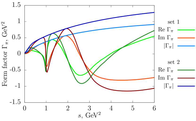
Figure 1: Real, imaginary parts and the absolute value of $\Gamma_{\pi}$ for the fitting sets 1 and 2 of Tab. 2.

Remarkably, both fits at $s\to 0$ approach the leading order prediction of ChPT (11). With $x\equiv M_{S}^{2}/1$ GeV² we obtain a numerical approximation for the average between set 1 and set 2:

$$|\Gamma_{\pi}|=(0.13+0.39x-0.062x^{2}+0.0041x^{3})\text{ GeV}^{2}.$$ (20)

3. The estimated form factor contributes to the total scalar decay rate to pions (the rate to neutral pions is half of the rate to charged ones) as

$$\Gamma(S\to\pi\pi)=\frac{3}{32\pi}\frac{49\xi^{2}\,|\Gamma_{\pi}(M_{S}^{2})|^{2}}{81\,v^{2}M_{S}}\,\beta(M_{S}^{2})$$ (21)

$$=(0.983+6.54x-1.12x^{2}+0.071x^{3})\cdot 10^{-8}\text{ GeV}\,,$$

while the leading order ChPT result is obtained from (21) by replacing $\Gamma_{\pi}\to G_{\pi}$, see (14). Both results are outlined in Fig. 2

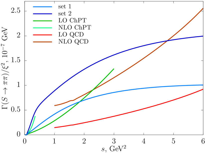
Figure 2: The decay width of hidden scalar to pions calculated using $\Gamma_{\pi}$ from Fig. 1 for the fitting sets 1 and 2 (light and dark blue lines) and ChPT (green line) divided by $\xi^{2}$. Light green line shows the decay width to pions divided by $\xi^{2}$ obtained using the NLO ChPT results for $\Gamma_{\pi}$ and $T_{\pi}$ Gasser and Leutwyler (1984); Kubis and Meissner (2000). The result of LO (NLO Djouadi et al. (1991)) QCD calculation for the decay width of the hidden scalar to gluons is shown in red (dark orange), the renormalization scale is $\sqrt{s}\equiv M_{S}$.

along with the leading-order QCD calculations of the decay rate into gluons (5) and the next-to-leading order ones calculated for the light Higgs boson at the renormalization scale $\mu=M_{S}$ Djouadi et al. (1991). There is also shown the decay width obtained using the NLO ChPT result for $\Gamma_{\pi}$ and $T_{\pi}$ Gasser and Leutwyler (1984); Kubis and Meissner (2000). We observe, that with our estimate of $\Gamma_{\pi}$ the decay rate to pions reasonably matches that into gluons at $M_{S}\simeq$ 1.5-2 GeV (light quark contribution (4) is negligible), and in this mass range the total ChPT leading order estimate reveals similar result. One may therefore speak on ”gluon-hadron” (or in some sense ”quark-gluon”, as the pions are obviously quark states) duality. While the smaller fitting curve seems to be preferable, the deviations by no means may substantially exceed a factor of two, still consisting with uncertainties we expect in the fitting and calculations. One should bear in mind that the ChPT expansion is valid only up to dark scalar masses of order 1 GeV, although we extend the green line in Fig. 2 to higher $s$ in order to demonstrate the overlapping of the results.

Note that the scalar form factor behaviour within dispersion approach and ChPT were systematically compared in Sec. 2 of Colangelo (2002). While both NNLO contribution of ChPT and the dispersion relation provide a decrease of $\Gamma_{\pi}(s)$ at $s\sim(0.5\,\textrm{GeV})^{2}$, there is a quantitative discrepancy due to an underestimate of phase in ChPT. Moreover, at $s\sim 1\,\textrm{GeV}^{2}$ the phase evaluation in the Omnes approach should be strongly violated by the contributions of inelastic channels, in particular, $KK$, making their account rather important. Indeed $\Gamma_{\pi}$ exhibits much lower peak within 2-channels analysis Bezrukov et al. (2018).

Contrary to estimates of Donoghue et al. (1990), our result for the decay rate as a function of scalar mass does not exhibit any peak-like structures, which might be attributed to the impacts of light scalar hadronic resonances. We find that impacts of some, in particular $f_{0}(500)$ and $f_{2}(1270)$, are small, while some, e.g. $f_{0}(980)$, are not seen in the fit Kumano et al. (2018) and hence do not interfere in (8) being most probably bound states of four quarks. Note in passing that operator $m\bar{q}q$ contributes also to $T_{\pi}$. Its account implies the replacement $49/81\to 1$ in eq. (21).

4. The calculated decay rate of the hidden scalar into pions can be used along the decay rates into photons, leptons, etc, see e.g. Bezrukov and Gorbunov (2010), to evaluate the light scalar lifetime and entire pattern of branching ratios of the light scalar decays into the SM particles, see Fig. 3.

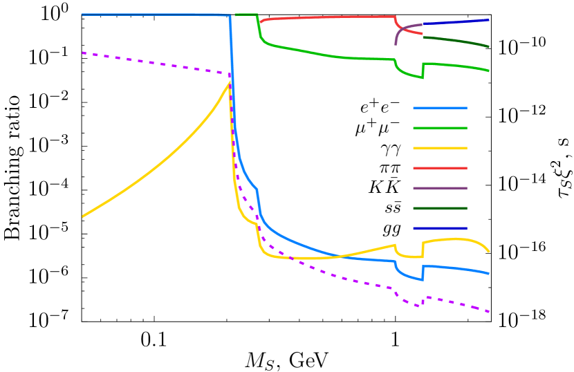
Figure 3: Branching ratios of hidden scalar to leptons, photon pairs, pions (using the result of this work), kaons (within the framework of ChPT), $s\bar{s}$ pairs and gluons (NLO QCD calculation). The branchings are shown with solid lines. The dashed line shows hidden scalar lifetime multiplied by $\xi^{2}$.

Here for $\Gamma_{\pi}(s)$ we use (20). In the mass region $M_{S}\sim 1$ GeV we expect uncertainties by a factor of 2-3 due to uncertainties in the gravitational form factor we used and due to our disregard of the gluonic contribution to the latter. It might be partially accounted along the quark contribution in the analysis of Ref. Kumano et al. (2018), which deserves an elaboration. We do not expect any induced by gluons features in the scalar decay rate to hadrons provided no light scalar resonances consisted of gluons. We use the corrected pattern in Fig. 3 to refine the experimental reach in the model parameter space as presented in Fig. 4.

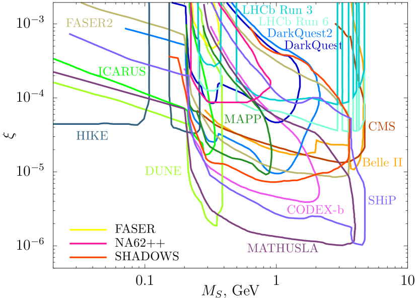
Figure 4: Expected reach of existing and proposed experiments in the model parameter space updated in accordance with the result for decay rate to pions. Peaks of original curves from Batell et al. (2022) corresponding to the resonance enhancement of $\Gamma(S\to\pi\pi)$ have been smoothed accordingly.

To further improve the accuracy in calculation of the scalar decay rates to hadrons, it is worth to infer other hadronic gravitational form factors, possibly from analyses of $\gamma^{*}\gamma\to KK$, $\gamma^{*}\gamma\to\eta\eta$ scatterings or $J/\psi\to\gamma+\pi\pi$, etc, decays collected at $c$- and $b$-factories.