An Empirical Analysis of the Shift and Scale Parameters in BatchNorm

Abstract

Batch Normalization (BatchNorm) is a technique that improves the training of deep neural networks, especially Convolutional Neural Networks (CNN). It has been empirically demonstrated that BatchNorm increases performance, stability, and accuracy, although the reasons for such improvements are unclear. BatchNorm includes a normalization step as well as trainable shift and scale parameters. In this paper, we empirically examine the relative contribution to the success of BatchNorm of the normalization step, as compared to the re-parameterization via shifting and scaling. To conduct our experiments, we implement two new optimizers in PyTorch, namely, a version of BatchNorm that we refer to as AffineLayer, which includes the re-parameterization step without normalization, and a version with just the normalization step, that we call BatchNorm-minus. We compare the performance of our AffineLayer and BatchNorm-minus implementations to standard BatchNorm, and we also compare these to the case where no batch normalization is used. We experiment with four ResNet architectures (ResNet18, ResNet34, ResNet50, and ResNet101) over a standard image dataset and multiple batch sizes. Among other findings, we provide empirical evidence that the success of BatchNorm may derive primarily from improved weight initialization.

1 Introduction

In recent years, computational advances have resulted in the ability to train deeper networks, which has led to increases in classification accuracy on many tasks [2]. This has allowed for the use of deep learning for problems that had previously been considered extremely difficult. One such example is the use of deep Convolutional Neural Networks (CNN) for image classification. CNNs apply filters—also called kernels—to images to extract high level features such as edges. Modern CNNs can use many such layers, which can increase their classification accuracy. However, deeper networks come with a set of challenges [5]. For example, in deep networks, overfitting is often problematic, and convergence can become harder to achieve. In addition, deeper networks are more likely to result in so-called vanishing and exploding gradients. These gradient issues arise due to products of weights that are computed. In order to avoid these pitfalls, a number of approaches have been suggested with, arguably, the most notable being Batch Normalization (BatchNorm).

In a CNN, BatchNorm can be viewed as a layer that we insert between convolutional layers. In effect, BatchNorm is a statistical regularization process, where we obtain a standardized output for each node in a layer. The mean $\mu$ and standard deviation $\sigma$ for a given neuron in a given layer is determined over an entire batch. Then we normalize so that $(\mu,\sigma)=(0,1)$, and we compute the $z$-score. This $z$-score measures how far—in terms of standard deviation units—the input to the neuron is from the norm. The $z$-score is then multiplied by a parameter $\gamma$, added to another parameter $\beta$, and the result of this affine transformation is passed on to the next layer. The parameters $\gamma$ and $\beta$ are learned via training through backpropagation, along with the CNN weights.

When BatchNorm was proposed in 2015, it was hailed as a breakthrough that unlocked the ability to develop networks with much greater complexity that did not experience the degradation in performance that had previously been observed [10]. The use of BatchNorm yields an empirical increase in training accuracy, a reduction in the number of training steps, and it improves overfitting, in the sense of decreasing the number of dropout layers that are required. However, it is not clear why BatchNorm produces such improvements. The original authors of BatchNorm plausibly suggested that the reason for the success of the technique was a reduction in the Internal Covariate Shift (ICS) [10].

ICS is defined as “the change in the distribution of network activations due to the change in network parameters during training” [10]. In effect, each layer “sees” its input as statistically differently, and the more layers, the greater this effect is likely to be. In backpropagation, such differences can lead to inconsistent updates—when gradient descent is used to modify the weights of a layer, there is an implicit assumption that the other layers have remained static [6].

In its original formulation, a BatchNorm layer was placed before an activation function, which would serve to make the input to each layer statistically similar, thus reducing ICS and thereby improving the representational power of the overall network. However, there is empirical evidence that placing the BatchNorm layer after the activation function achieves better results. This contradicts the original justification for BatchNorm, since the statistics of the inputs are not normalized. One attempt at analyzing BatchNorm injected noise into the data before the activation layers to skew the statistics of the layer—and thereby induce ICS—and found that there was no significant reduction in training accuracy as compared to standard BatchNorm [21]. The authors of [21] argue that what BatchNorm is really doing is re-parameterizing the model in a way that serves to smooth the loss surface and thereby accelerate convergence. They further posit that ICS may not even be an issue that needs to be addressed when training a neural network. Another study claimed that the speed and stability of BatchNorm are independent effects [4].

There are many alternatives to BatchNorm, with the normalization procedure taking place over differing attributes, e.g., normalization over layers, weights, and color channels each provide improvement, as compared to a standard model with no normalization. Many of these BatchNorm alternatives include shift and scale parameters, which serve to re-parameterize the data [16, 17, 20, 23, 27].

In this paper, we investigate the relationship between the re-parameterization in BatchNorm, and the normalization itself. The shift and scale parameters provide two additional trainable parameters—and hence two additional degrees of freedom—for each layer, which could account for some of the improvements observed in BatchNorm. To isolate the role of these parameters, we have produced a package that we call AffineLayer, which foregoes the normalization in BatchNorm and only performs the shift and scale re-parametrization step.

We have also produced a package that we call BatchNorm-minus that includes the normalization step of BatchNorm, but not the shift and scale re-parameterization. By comparing our AffineLayer and BatchNorm-minus results to BatchNorm, we hope to obtain insight into the relative contribution of the normalization step, as compared to the re-parameterization step, with the ultimate goal of shedding further light on the mechanism by which BatchNorm improves the training of models.

The remainder of this paper is organized as follows. In Section 2, we discuss relevant background topics, including the development of BatchNorm and previous attempts that have been made to understand why it works. We also discuss several alternatives to BatchNorm that have been previously developed. Section 3 focuses on our experimental design and provides implementation details. In Section 4, we give our experimental results and discuss our findings. We conclude the paper in Section 5, where we also consider directions for possible future work.

2 Background

This section deals with the details of BatchNorm, the principles behind it, some potential reasons for why it works, and alternatives to BatchNorm. We also discuss why ResNet was chosen for this research and the contributions of this research paper.

2.1 How BatchNorm Works

BatchNorm is an optimization and re-parametrization procedure performed per mini-batch. It consists of a normalization step that is based on the statistics of each mini-batch, along with per-layer shift and scale parameters. During the validation phase, the shift and scale parameters from the training phase are used to evaluate inputs.

2.1.1 Mathematics of BatchNorm

BatchNorm operates on every individual feature per mini-batch. For each feature $x_{j}$, we calculate the mean and variance as

$$\mu_{j}=\frac{1}{m}\sum_{i=1}^{m}x_{ij}\mbox{\ \ and\ \ }{\sigma_{j}}^{2}=\frac{1}{m}\sum_{i=1}^{m}{(x_{ij}-\mu_{j})}^{2}$$

respectively. We then uses these values to determine the $z$-score

$$\widehat{x}_{j}=\frac{x_{ij}-\mu_{j}}{\sqrt{{\sigma_{j}}^{2}+\varepsilon}}$$

where $\varepsilon$ is a constant for stabilizing the output Finally, we calculate the output

$$y_{j}=\gamma_{\ell}\kern 1.0pt\widehat{x}_{j}+\beta_{\ell}$$

where $\gamma_{\ell}$ and $\beta_{\ell}$ are per-layer parameters that are updated through backpropagation, alongside the weights.

According to the original BatchNorm paper [10], the purpose of the scale and shift parameters $\gamma$ and $\beta$ is to restore information that may be lost through the normalization process of zeroing the mean. This scale and shift serves to re-parametrize the activations in a way that allows for the same family of functions to be expressed, but with trainable parameter that may make it easier to learn via gradient descent [6].

2.1.2 Internal Covariate Shift

Internal Covariate Shift (ICS) is a known issue for deep neural nets. The more layers the neural network has, the more the statistics of each layer change as a result of the preceding layers and, more specifically, the distribution of the activation functions change as more updates are performed. In backpropagation, when parameters are updated, all layers are updated simultaneously, under the implicit assumption that the statistics of previous layers are static [6]. The “covariate” refers to the way that the inputs to the neural network vary relative to each other, while the “shift” refers to the change in the distributions of the outputs across different layers. The effect of ICS on statistical predictions predates neural networks [22]. In the context of neural networking, ICS has also been discussed with respect to distribution changes between the training and validation domains [11].

2.1.3 What is BatchNorm Trying to Achieve?

There is no rigorous proof as to why BatchNorm improves the performance of deep neural networks, nor is there a consensus on why the technique is so successful. BatchNorm has been shown empirically to regulate overfitting and reduce or eliminate the need for dropout layers.

A large learning rate can cause erratic training behavior, but a learning rate that is too small can cause a model to fail to converge or to require more training epochs. BatchNorm allows for a smaller learning rate with no loss in performance, and it seems to perform better with a batch size of 30 or more. The creators of BatchNorm posited that it could be reducing the ICS and hence it works by reducing the “randomness” that occurs in each batch of data as a consequence of simultaneous updates over many layers [10].

Where to place the BatchNorm layers within a CNN has been a topic of much debate. The original paper places BatchNorm layers before the activation function, which is supposed to improve ICS and thereby reduce vanishing or exploding gradient issues during training. However, in practice it has been observed that BatchNorm performs as well—or even better—when it is applied to the output of the activation function. This would seem to contradict the stated purpose of the parameters $\beta$ and $\gamma$, which are supposed to control the statistics of the layer, since that ability is reduced when the output is passed through the activation function prior to BatchNorm.

There are published research papers, including [9, 10, 11], that argue that BatchNorm works because it reduces ICS and acts like a normalizer. However, there are other papers, such as [8, 21], that provide evidence that ICS is not even a real issue for neural networks, and that BatchNorm is just smoothing the gradient landscape and thereby accelerating convergence. Part of the evidence for this latter perspective is that we can place the BatchNorm layer anywhere and obtain improvements, as compared to no such normalization. Others make the argument that BatchNorm smoothes out the loss surface, which makes it easier to reach a global maximum [21].

In this paper, we conduct experiments that attempt to separate out the relative effect of the two components of BatchNorm, namely, the normalization step and the re-parameterization via the trainable parameters $\gamma$ and $\beta$. By considering these components separately, as detailed in Section 3.2 below, we hope to gain insight into how and why BatchNorm is so effective. As far as the authors are aware, this is a novel approach to analyzing BatchNorm.

2.2 Datasets

The Canadian Institute for Advanced Research 10-class dataset, commonly referred to as CIFAR10 [15], is comprised of 60,000 images, each of which is a $32\times 32$ pixel image. Alongside ImageNet, it is one of the most widely used datasets for machine learning and deep learning research. The CIFAR10 dataset consists of 50,000 training images (5000 from each of the 10 classes), and 10,000 validation images (1000 from each class). The 10 mutually exclusive classes are airplane, automobile, bird, cat, deer, dog, frog, horse, ship, and truck. Also, each image only contains the specified object. This dataset is available as part of the PyTorch [19] package. An example of a CIFAR10 image is given in Figure 1.

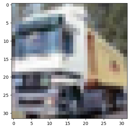
Figure 1: Example of CIFAR10 image of truck

In this paper, we use the CIFAR10 dataset for our experiments. CIFAR10 has been considered in several other research papers that attempt to evaluate BatchNorm.

2.3 ResNet

We use Residual Networks (ResNet) for our experiments, in part because ResNet was developed with BatchNorm built into it. Papers evaluating BatchNorm or its variants typically choose ResNet for this reason, as well as it being one of the current best classifiers [24].

ResNet was developed in 2015 and it can be viewed as a type of Convolutional Neural Network (CNN). As alluded to above, ResNet is considered the current state of the art in computer vision [7], as it consistently outperforms its competitors in competitions involving image tasks. A ResNet architectures uses a series of repeating blocks made from convolution layers that are designed to model the “residual function” instead of the output. Here, the residual function is defined as the difference between the input and the output of a residual block. If the input is $x$ and the output is $F(x)$ then the residual being modeled is $F(x)-x$. The motivation behind ResNet was the observation that deeper networks sometimes performed worse than shallower networks, which is counterintuitive, as “excess” layers should simply model the identity function. By modeling the residual, ResNet blocks model the identity function as 0, which may be easier to learn via backpropagation.

Each residual block in a ResNet has two pathways, namely, the residual mapping or an identity mapping, where the identity mapping implies that the block is, in effective, being skipped over, thus improving gradient flow through the remainder of the network. This makes deeper networks more feasible—ResNets can be trained with vastly more layers as compared to traditional neural networks. Residual blocks also serve to decrease overfitting. In practice, ResNet appears to act as a collection of shallow neural nets—in effect, an ensemble that is trained simultaneously [24].

ResNet uses Rectified Linear Unit (ReLu) activations, which have been empirically shown to decrease the incidence of vanishing gradients. In addition, ResNet makes use of BatchNorm before each activation function. Each specific ResNet architecture is specified as “ResNet$n$”, where $n$ denotes the number of convolution layers in the ResNet. Popular ResNet architectures include ResNet18, ResNet34, ResNet50, ResNet101, ResNet110, ResNet152, ResNet164, and ResNet1202. Note that, in general, the residual block structure in different ResNet architectures differ.

As mentioned above, ResNet architectures utilize BatchNorm within residual blocks, and the contribution of BatchNorm to the success of these architectures is well documented. These factors makes ResNet an ideal candidate for our experiments, where we attempt to understand the relative contributions of the components of BatchNorm (i.e., normalization and re-parameterization).

In this research, we consider ResNet18, ResNet34, ResNet50, and ResNet101. All of these achieve reasonably high accuracies on the CIFAR10 dataset. These architectures use different residual blocks: ResNet18 and ResNet34 use smaller two-convolution layer blocks called basic blocks, while ResNet50 and ResNet101 use three-convolution layer blocks called bottleneck blocks. The bottleneck blocks in ResNet50 and ResNet101 reduce the dimensionality of the 256 dimensional input before applying $3\times 3$ convolution filters, the result of which is then projected back into 256 dimensions. Basic blocks and bottleneck blocks are illustrated in Figures 2.3(a) and (b), respectively.

& (a) Basic block (b) Bottleneck block

Figure 2: Residual blocks in selected ResNet architectures

Since these four architectures perform comparably well on the CIFAR datasets, they will help us to determine whether our empirical results are dependent on the depth of the ResNet. Also, since there are two different block structures among the four architectures under consideration, we can observe the effect of the block type, relative to the components of BatchNorm.

2.4 Related Work

In this section, we consider relevant related research that has attempted to demystify BatchNorm, summarizing the methods used and the results that were obtained. We also consider a few BatchNorm alternatives and discuss how they achieve their results.

2.4.1 Refuting ICS

In the 2018 paper [21], evidence is provided that the success of BatchNorm is not due to ICS at all, and that it might not even be reducing ICS. To support this hypothesis, based on a VGG classifier and CIFAR10, they injected noise into the activations following each BatchNorm layer so that any mitigation of ICS that BatchNorm might have provided was no longer valid. This noise was randomized at each time step so that none of the distributions were identical. These experiments showed that there was no drop in performance between the noise-injected network and the one with standard BatchNorm. In addition, both networks significantly outperformed a VGG neural net that did not use BatchNorm. This contradicts the original BatchNorm paper; if ICS reduction was the main benefit of BatchNorm, then adding ICS to a network would degrade its performance. In contrast, these experiments show that BatchNorm improves the performance of VGG, even when ICS is increasing.

In the paper [21], the authors also proposed a more precise definition for ICS in the context of neural networking. ICS should be reflected in how much a neural networking layer needs to adapt to changes in its inputs. Therefore, they quantify ICS as the difference between $G$ and $G^{\prime}$, where $G$ consists of the gradient parameters before updates and $G^{\prime}$ consists of these same set of parameters after the updates. They measured this difference in terms of the $L_{2}$ norm and cosine similarity.

If BatchNorm was indeed reducing ICS, as defined by the metric in the previous paragraph, then the use of BatchNorm layers would decrease the correlation between $G$ and $G^{\prime}$ since BatchNorm would cause less cross-layer dependency. However, the authors of [21] obtained the surprising result that a network with BatchNorm was increasing the correlation between these variables. The authors believe that this occurs because BatchNorm effectively re-parameterizes the loss function, and hence its impact is likely due to an improvement in this surface. That is, BatchNorm could be smoothing the loss surface, making it easier for gradient descent to reach the desired outcome. To verify this, they considered the “Lipschitzness” of the loss function with and without BatchNorm.

A function $f$ is $K$-Lipschitz provided that ∥ f(x_1) - f(x_2)∥ ≤K ∥ x_1 - x_2 ∥ for all choices of $x_{1}$ and $x_{2}$, where $K$ is real-valued, with $K>0$. Lipschitz continuity means that the function is strongly uniform continuous and $K$ provides a limit on how rapidly it can change. A larger $K$ implies a smoother loss function, which is a good thing with respect to convergence via gradient descent.

The authors of [21] discovered that BatchNorm did not just improve the Lipschitzness of the loss function but also the Lipschitzness of its gradients, which implies increased convexity. This makes a strong case for the underlying mechanics of BatchNorm, but it does not settle which aspects of BatchNorm lead to the improvements. It could simply be the case that the addition of more trainable parameters (i.e., shift and scale) helps, since it is theorized that having more parameters might explain some of the performance disparity between shallow and deep networks [2].

2.4.2 Further Experiments on the ICS

In the 2020 paper [9], the authors claim to improve BatchNorm by using an alternative metric for ICS, and they determine upper and lower bounds for the ICS. They use the so-called earth mover’s distance, a measure that quantifies the distance between two probability distributions. In this case, the distributions being compared are based on the statistics of the gradient values before and after updates. The paper claims to obtain an improvement over BatchNorm, albeit a small one. Interestingly, their normalization step involves an additional parameter $\alpha$, which is trained alongside the $\beta$ and $\gamma$ parameters. They tested their algorithm on various ResNets [1].

2.4.3 Regularization and BatchNorm

In the 2018 paper [18], population statistics were used instead of batch statistics, and a regularization term was included for the $\gamma$ parameter. In these experiments, it was noted that for batches of size larger than 32, the population statistics function as well as the batch statistics. It was also noted that BatchNorm introduces Gaussian noise into the mean and variance parameters. The algorithm in [18] produces accuracies that are comparable to BatchNorm, but unlike the case with BatchNorm, they found that introducing dropout layers improved performance further. They also state that BatchNorm has very similar effects to $L^{p}$ norm regularization where the $p$-norm is defined as ∥x_p∥ = (∑_i=1^n —x_i—^p)^1/p ​.

If $L^{p}$ norm regularization was sufficient, there would be no need for an optimization such as BatchNorm, since regularization is less computationally intensive. However, this regularization claim is not consistent with other empirical studies, such as that presented in the 2018 paper [25].

2.4.4 Weight Normalization and BatchNorm

While BatchNorm deals with the input to activation functions in a layer, it would be reasonable to attempt to normalize the weights of a layer directly [20]. This WeightNorm approach works per batch, similar to BatchNorm but claims to be less noisy and more computationally efficient, especially for shallower networks. In WeightNorm, the weight vector is re-parametrized as w = g∥v∥ v where $g$ is a trainable parameter and $\|v\|$ is the Euclidean norm of $v$. The authors of [20] combine this with a form of BatchNorm, meant only to center the gradients. This is referred to as “mean-only BatchNorm”, where only the mean of the neuron inputs is calculated. The authors of WeightNorm emphasize that one advantage of their normalization is that it decouples the direction of the weight vector from its magnitude, and this has led to speculation that the performance of BatchNorm is also due to this property [14].

2.4.5 Decoupling the Length and Direction of the Weights

In [14], it is shown that the transformations that BatchNorm imposes results in the magnitude of the weight vector being independent of the direction of the vector. The authors hypothesize that this allows BatchNorm to use properties of the optimization landscape in a way that other regularization methods cannot. Using this property in their optimization step, they were able to achieve a linear convergence on a non-convex problem.

2.4.6 Residual Learning without Normalization

Another way in which BatchNorm could be improving deep neural nets is by making the weight initializations more consistent at the start of each epoch. The weight initialization problem had been discussed before the inception of BatchNorm [5]. In 2019, a paper based on research done at Facebook developed a method called Fixup Initialization [28]. This method is another attempt to solve the exploding and vanishing gradient issue, which is related to the fact that the deeper the neural net, the larger the variance of its output will tend to be. Fixup introduces a rescaling of the standard weight initializations and it also includes trainable shift and scale parameter similar to BatchNorm. The authors claim that using their Fixup, they can obtain results that are superior to BatchNorm on the CIFAR10 dataset, based on a ResNet architecture. Given that they also use shift and scale parameters, this does not have clear implications for the effective mechanism behind BatchNorm.

2.4.7 Decorrelated Batch Normalization

One of the motivations behind the development of BatchNorm was the idea that inputs to the activations should be whitened, which requires scaling, standardizing, and decorrelating. BatchNorm however only implements the first two, because it is computationally intensive to decorrelate—this would require computing the inverse square root of the covariance matrix during back propagation [13]. The 2018 paper [8] implements what the authors call “Decorrelated BatchNorm” through a process called Zero Phase Component Analysis. This process involves scaling along eigenvectors, and is similar to Principal Component Analysis, except that it but does not rotate the coordinate axes. The authors use the transformation ^x_i = $\Sigma^{1/2}$(x_i - μ) where $\mu$ is the mean of the mini-batch and $\Sigma$ is the covariance matrix of the mini batch.

Testing on CIFAR10, and the more challenging CIFAR100 dataset, using ResNet the authors of [8] note that the whitening process creates an improvement in performance over vanilla BatchNorm. They also recommend including shift and scale parameters, since these also improved performance. However, the computational cost of whitening is non-trivial.

2.4.8 Adaptive Batch Normalization

Adaptive Batch Normalization (AdaBN) improves on BatchNorm in transfer learning applications [16]. One of the issues with BatchNorm is that there is a disconnect between source and target domains, in the sense that the statistics used for each differ. Here, the source is the data the weights are derived from, while the target is the new data that we are classifying. AdaBN uses the BatchNorm statistics and combines them with weight statistics, with the rationale being that BatchNorm statistics provide information about the source, while the weight statistics provide information about the target. For neuron $j$ and for an image $m$ in the dataset, they calculate y_j(m) = γ_j xj(m) - μjtαjt + β_j where $\mu_{j}^{t}$ and $\alpha_{j}^{t}$ are, respectively, the mean and variance of the outputs of the neuron in the target domain.

2.4.9 AutoDIAL: Automatic DomaIn Alignment Layers

Another transfer learning algorithm is AutoDIAL [3], which attempts to maximize classification accuracy by aligning the source and target domains. They do so by looking at statistics from both domains in advance and designing a parameter $\theta$ that represents the shared weights. They still use BatchNorm layers to bring the two domain together but they do so via a parameter $\alpha$ that quantifies the degree of mixing of both sets of statistics. If $\alpha=1$, then the domains are not aligned while $\alpha=0.5$ indicates that they are partially aligned.

2.4.10 Layer Normalization

LayerNorm functions within a mini-batch, where it is trying to normalize the inputs with respect to the other features in the same layer of the neural network [27]. This approach uses the same statistics as BatchNorm but whereas BatchNorm is based on the same feature, LayerNorm is computed across different features. This works best when the features are similar to each other in scale. LayerNorm has been used successfully in Recurrent Neural Networks (RNN) and transformers-based machine learning models. Since it functions per layer, unlike BatchNorm, there are no dependencies between layers and hence LayerNorm would not be expected to result in any decrease of ICS within a network.

2.4.11 Instance Normalization

InstanceNorm is a variation of LayerNorm that works across RGB channels instead of features [27]. This is an attempt at maximizing contrast within images and it has been applied with success to GANs.

2.4.12 Group Normalization

GroupNorm was created to allow for smaller batch sizes, as compared to standard BatchNorm [26]. For high-resolution images, smaller batches of size one or two are preferred, whereas BatchNorm requires larger batch sizes to perform well. GroupNorm, does not normalize in batches, but instead normalizes along the feature dimension by considering groups of features. GroupNorm has been shown to work well for batches of size two, and it may enhance object segmentation and detection.

2.4.13 SwitchBlade Normalization

SwitchBlade Normalization (SN) combines three approaches that we have discussed above [17]. Specifically, SN combines InstanceNorm (to normalize across each feature), LayerNorm (to normalize across each layer), and BatchNorm (to normalize across each batch). The algorithm learns which of the three types of normalizations works best with the data and can “switch” between any combination of the three that achieves the best result. The authors of SN note that of the three normalizations, BatchNorm is assigned the highest weight during image classification tasks.

3 Experimental Design

In this section, we present our experimental process from a high-level perspective. Specifically, we discuss the design of our BatchNorm variants, our PyTorch implementations, and the hyperparameters selected for the experiments presented in Section 4.

3.1 Architecture Selection

Above, we explained that ResNet was chosen for our experiments because it is the current best image classifier and it is heavily dependent on BatchNorm. ResNet also comes in multiple variants, enabling us to easily experiment with different depths and different residual block structures. Based on preliminary tests, we chose to focus on ResNet18, ResNet34, ResNet50, and ResNet101, since these models are fast to train, and they are sufficient to illustrate the key points of our research. Recall that ResNet18 and ResNet34 use basic residual blocks, while ResNet50 and ResNet101 use bottleneck blocks, as illustrated in Figure 2.3, above. Hence, ResNet34 can be viewed as a deeper version of ResNet18, and the same can be said of the pair ResNet101 and ResNet50. However, ResNet50 is not just a deeper version of ResNet18, for example.

3.2 BatchNorm Variants

As mentioned above, we have implemented two BatchNorm variants that are designed to help us determine the relative contributions of the normalization step, as compared to the re-parameterization step. The first of these, which we refer to as AffineLayer, includes only the affine transformation part of BatchNorm. That is, AffineLayer does not normalize the output, but does include trainable shift and scale parameters ($\gamma$ and $\beta$, respectively). These parameters offer two additional degrees of freedom for each neuron, which may allowing for more expressive models. We also develop and analyze a variant that includes the normalization step of BatchNorm, but not the re-parameterization, which we refer to as BatchNorm-minus. We compare these techniques to standard BatchNorm and to the case where no normalization is use, which we denote as “none” in our tables and graphs. Table 1 summarizes the four variations that we test on the ResNet18, ResNet34, ResNet50, and ResNet101 networks.

Table 1: Normalizations tested

Normalization Re-parameterize Re-normalize ($\beta$ and $\gamma$) BatchNorm ✓ ✓ AffineLayer ✓ ✗ BatchNorm-minus ✗ ✓ None ✗ ✗

Tables 2 and 3 summarize the hyperparameters tested (via grid search) for the ResNet architectures under consideration. In both of these tables, boldface is used to indicate the hyperparameter value that yields the best result. Note that in every case, the Adam optimizer is best, as is a learning rate of $0.001$, while the best choice for batch size varies considerably. Therefore, for all experiments in Section 4, we use the Adam optimizer and a learning rate of $0.001$, and all models are trained for 15 epochs. To reduce the number of potential confounding variables, we only consider batch sizes of 20 and 50. Thus, our experiments will not necessarily yield the best possible accuracies, but that is not our purpose. Instead, our goal to highlight differences between the ResNet models, relative to the four normalization schemes under consideration.

Table 2: Hyperparameters for ResNet18 and ResNet34

Normalization Hyperparameter Values tested Best validation accuracy BatchNorm Learning rate 0.01,0.005,0.001 0.7665 Optimizer Adam, SGD Batch size $20,30,\ldots,100$ (30) AffineLayer Learning rate 0.01,0.005,0.001 0.6904 Optimizer Adam, SGD Batch size $20,30,\ldots,100$ (80) BatchNorm-minus Learning rate 0.01,0.005,0.001 0.7730 Optimizer Adam, SGD Batch size $20,30,\ldots,100$ (20) None Learning rate 0.01,0.005,0.001 0.6877 Optimizer Adam, SGD Batch size $20,30,\ldots,100$ (80)

Table 3: Hyperparameters for ResNet50 and ResNet101

Normalization Hyperparameter Values tested Best validation accuracy BatchNorm Learning rate 0.01,0.005,0.001 0.7469 Optimizer Adam, SGD Batch size $20,30,\ldots,100$ (70) AffineLayer Learning rate 0.01,0.005,0.001 0.6986 Optimizer Adam, SGD Batch size $20,30,\ldots,100$ (80) BatchNorm-minus Learning rate 0.01,0.005,0.001 0.6540 Optimizer Adam, SGD Batch size $20,30,\ldots,100$ (100) None Learning rate 0.01,0.005,0.001 0.6939 Optimizer Adam, SGD Batch size $20,30,\ldots,100$ (70)

3.3 Implementation

We conduct our experiments using PyTorch, an open source machine learning library, which is itself based on the Torch package. For our purposes, the main benefit of PyTorch comes from its use of tensors, which are auto-differentiable numerical arrays that allow GPU parallelized Basic Linear Algebra Subprograms (BLAS) operations [19]. This enables us to implement our AffineLayer as a tensor layer in the form of a custom PyTorch nn.module, which is one of the base classes. The two parameters, $\beta$ and $\gamma$, are tensors and can be multiplied and added to the input layer. Defining $\beta$ and $\gamma$ as nn.Parameter, which is a type of array, makes them part of the computational graph which enables them to be trained via backpropagation. PyTorch is also convenient for our purposes because it offers a ResNet builder function that lets the user select which optimization layer to pass to the builder as an argument.

To implement BatchNorm-minus, we modified the existing BatchNorm layer in PyTorch to make the shift and scale no longer trainable, which leaves them at their initial values of $(\beta,\gamma)=(0,1)$. To train our models without any type of normalization (which is denoted as “none” in our tables and graphs), we simply use an identity layer in place of BatchNorm.

Finally, all of our experiments have been run on an RTX3080Ti GPU and take on average two minutes per epoch to complete. Since our hardware enables fast training, we are able to conduct a large number of experiments.

4 Experimental Results

In this section, we compare the four different normalizations discussed above, namely, BatchNorm, AffineLayer, BatchNorm-minus, and “none” (i.e., no normalization). First, we give results for the ResNet18 and ResNet50 architectures, then we consider ResNet34 and ResNet101. We also provide an in-depth analysis of gradient and weight statistics for our models, and we conclude this section with a discussion of our experimental results.

4.1 ResNet18 and ResNet50 Experiments

As with all of our experiments, for the ResNet18 and ResNet50 models, we use the CIFAR10 dataset. These two architectures are the shallowest of their respective types, with ResNet18 using basic residual blocks and ResNet50 using bottleneck residuals blocks. Our experiments with these models provide a point of comparison between the two types of blocks and also enable us to see how depth affects the results. Following our experiments with these models, we further experiment with the ResNet34 and ResNet101 architectures.

4.1.1 ResNet18 Results

Table 4 compares the four normalization—in terms of validation accuracy—based on the average of four different runs of each. The differences between batch sizes of 20 and 50 are marginal.

Table 4: ResNet18 experimental results

Normalization Validation accuracy Batch size 20 Batch size 50 BatchNorm 0.7665 0.7569 AffineLayer 0.6794 0.6904 BatchNorm-minus 0.7730 0.7644 None 0.6643 0.6877

From Table 4 we observe that BatchNorm-minus achieves slightly better results than BatchNorm. Recall that for BatchNorm-minus we found its optimal batch size to be 20, while 30 was optimal for BatchNorm. This suggests that for ResNet18, it may be better to use BatchNorm-minus, since a smaller batch sizes have been empirically linked to improved convergence properties [12]. Also, for ResNet18, our BatchNorm-minus results provide evidence that the shift and scale parameters are not as important as the normalization step.

4.1.2 ResNet50 Results

As can be observed by comparing Table 5 to Table 4, we obtain much different results with ResNet50 as compared to ResNet18. Specifically, the performance of BatchNorm-minus dropped dramatically, while BatchNorm is the best performer in the ResNet50 case. This could be due to the bottleneck architecture of ResNet50, which projects the convolution layers into a lower dimension before re-projecting them into their original dimensions.

Table 5: ResNet50 experimental results

Normalization Validation accuracy Batch size 20 Batch size 50 BatchNorm 0.7469 0.7424 AffineLayer 0.6957 0.6986 BatchNorm-minus 0.5597 0.6540 None 0.6786 0.6939

In contrast to BatchNorm-minus, the performance of AffineLayer increases for ResNet50, as compared to ResNet18. The parameters $\beta$ and $\gamma$ may be adding expressiveness back to the model. Lacking those additional training parameters, BatchNorm-minus has trouble converging, and even under-performs the case where no normalization is used.

We conjecture that the $1\times 1$ convolution of the ResNet50 bottleneck architecture is stripping the model of information, while the additional shift and scale parameters enable the model to recover some of that information. This would explain why the performance of BatchNorm-minus falls below AffineLayer. Whatever the reason, it appears that for ResNet50, the affine parameters play a much more significant role than in ResNet18. Another takeaway is that AffineLayer, which has no normalization step, is clearly outperforming BatchNorm-minus, regardless of the batch size. These results indicate that the normalization step is not the primary driver of improved performance in this case.

Note that the hypotheses that the success of BatchNorm is due to smoothing the loss surface [21] or decoupling the length and direction of the weight vectors [14] both are related to the normalization step. Since BatchNorm-minus performs poorly on ResNet50, our results indicate that these hypotheses fail to paint a complete picture, at least with respect to ResNet50. In the next section, we shall see that the same comment holds for ResNet101. Since both of these architectures use bottleneck blocks—whereas ResNet18 and ResNet34 do not—it is likely that this is a key factor.

4.2 ResNet34 and ResNet101 Experiments

In the previous section, we observed that BatchNorm-minus performs well with ResNet18, but poorly with ResNet50. One possible explanation for this difference is that the bottleneck block of ResNet50—which is not present in ResNet18—benefits from BatchNorm. To test this hypothesis, in this section we consider a series of experiments involving ResNet34 and ResNet101.

ResNet34 has the same general structure as ResNet50 and the same number of residual blocks but uses basic blocks instead of bottleneck blocks. Thus, other than the difference in depth, the primary difference between ResNet34 and ResNet50 is the block type. ResNet101 is a deeper version of ResNet50 with the same bottleneck block structure.

4.2.1 ResNet34 Results

Comparing the results for ResNet34 in Table 6 to those for ResNet18 in Table 4, we see more similarities than differences. In both cases, BatchNorm-minus marginally outperforms BatchNorm, with the other two cases trailing far behind This provides additional evidence that the bottleneck block affects the way that BatchNorm and its variants work.

Table 6: ResNet34 experimental results

Normalization Validation accuracy Batch size 20 Batch size 50 BatchNorm 0.7717 0.7554 AffineLayer 0.6856 0.6837 BatchNorm-minus 0.7719 0.7557 None 0.6661 0.6782

4.2.2 ResNet101 Results

The results in Table 7 for ResNet101 are analogous to what we observed for ResNet50. In this case, the performance for each normalization is worse than ResNet18 or ResNet34 and, crucially, the drop-off for BatchNorm-minus is large. AffineLayer is the best performer in this case. Since AffineLayer includes the two parameters that bring ICS back into the model, this is additional evidence that ICS reduction is not the reason for the success of BatchNorm. In fact, BatchNorm-minus would provide the tightest ICS control, and it gives us the worst results in this case.

Table 7: ResNet101 experimental results

Normalization Validation accuracy Batch size 20 Batch size 50 BatchNorm 0.6971 0.6746 AffineLayer 0.7032 0.6959 BatchNorm-minus 0.4412 0.4128 None 0.6819 0.6845

4.3 Analysis of Weights and Gradients

For ResNet18, we found that BatchNorm clearly outperformed AffineLayer; see Table 4, above. In an effort to better understand the reasons for the differing performance of these two normalization schemes, we extract the weights and gradients for the first epoch of ResNet18. Specifically, we consider the first and last layers of the ResNet18 model, based on the first 20 updates and the last 20 updates. We refer to these as “input” (first layer), “final” (last layer), “early” (first 20 updates), and “late” (last 20 updates). Here, we extract the weights and gradients for each of input-early, input-late, final-early, and final-late, and we plot various histograms of these distributions.

In Figure 3(a), we see that the weight distribution changes from input-early to final-late are fairly modest for BatchNorm, while Figure 3(b) yields the same conclusion for AffineLayer. In Figure 3(c), we have overlayed the final-late weights of BatchNorm and AffineLayer, while Figure 3(d) gives the analogous result for the gradients. We see that the weights and gradients behave similarly, and hence whatever is causing BatchNorm to outperform AffineLayer does not appear to be distinguishable through this weight and gradient distribution comparison. The bottom line here is that AffineLayer has a similar effect on the gradients as BatchNorm, at least in the all-important first epoch. Since AffineLayer performs significantly worse than BatchNorm, these results cast doubt on the claim that the success of BatchNorm is due to it stabilizing the gradients [10].

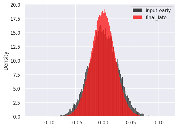
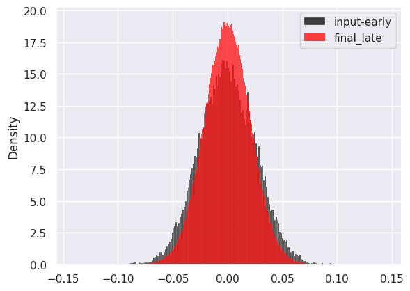
(a) BatchNorm weights		(b) AffineLayer weights
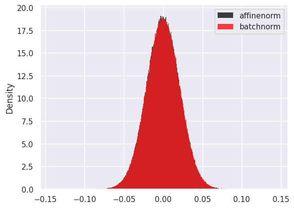
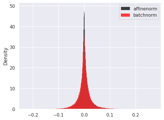
(c) Final-late weights		(d) Final-late gradients

Figure 3: Weight and gradient comparisons

The results in Figure 3 show minimal differences between BatchNorm and AffineLayer. A significant difference between AffineLayer and BatchNorm can be observed by comparing the input-early and input-late updates. Specifically, in Figure 4(a), we compare the input-early gradient with the input-late gradient for BatchNorm, while Figure 4(b) provides the analogous comparison for AffineLayer. We observe from Figure 4(a) that for BatchNorm, the gradient starts spread out and become more tightly focused, whereas Figure 4(b) shows the opposite behavior for the AffineLayer gradient.

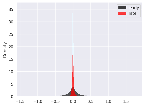
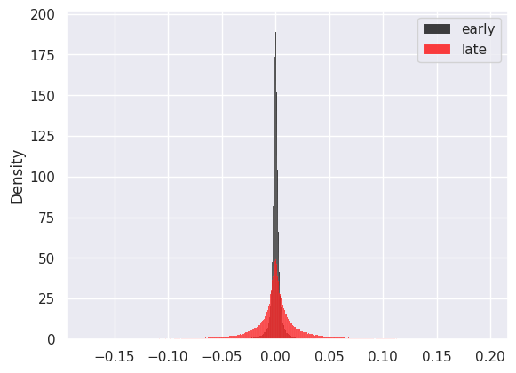
(a) BatchNorm		(b) AffineLayer

Figure 4: Gradients for input-early vs input-late

Figure 4 provides additional evidence that it is the weight normalization at the beginning of each epoch that is causing the observed performance differences between BatchNorm and AffineLayer, at least in the case of ResNet18. We discuss this further in the next section.

4.4 Discussion

In Figure 5, we summarize the results of our ResNet image classification experiments. Since we find minimal differences between the results for batch sizes of 20 and 50, for each model and normalization scheme, we have graphed the better of the results for batch size 20 or 50.

Figure 5: Summary of Results

From Figure 5, we note that for the models tested that employ basic blocks, namely, ResNet18 and ResNet34, BatchNorm-minus performs as well as standard BatchNorm. Since BatchNorm-minus normalizes the weights similarly to BatchNorm, this is consistent with the results in Figure 4, above. Also, since BatchNorm-minus lacks the trainable shift and scale parameters of BatchNorm, it appears that the additional degrees of freedom provided by these parameters are not particularly useful when training ResNet18 or ResNet34, and we conjecture that the same is true of any ResNet model that uses basic blocks. If this is the case, a simpler and more efficient normalization scheme can be used with such models, without any appreciable loss in performance.

On the other hand, for models tested that include bottleneck blocks, namely, ResNet50 and ResNet101, BatchNorm-minus performs relatively poorly. Hence, we conclude that the additional degrees of freedom provided by the shift and scale parameters are critical for these models, and we conjecture that the same is true of any ResNet that utilizes bottleneck blocks. Additional evidence that such is the case is provided by the fact that AffineLayer—which includes trainable shift and scale parameters—performs better on the bottleneck block architectures as compared to the basic block architectures.

5 Conclusion

A considerable body of previous research has focused on BatchNorm, but to the best of our knowledge, none has followed the approach in this paper, where the normalization and re-parameterization steps are separated and analyzed. We applied four distinct normalization schemes to each of ResNet18, ResNet34, ResNet50, and ResNet101, and presented a brief analysis of weights and gradients for ResNet18.

Our main results involve the relative contribution of the normalization and re-parameterization steps for the various ResNet architectures tested. Specifically, we found that for ResNet50 and ResNet101, the trainable shift and scale parameters appear to increase the expressiveness of the model, allowing it to recover more information after the dimensionality reduction step that occurs inside bottleneck residual blocks. In contrast, for ResNet18 and ResNet34 which use basic residual blocks, we found that normalization was beneficial, but that the additional degrees of freedom provided by shift and scale parameters did not improve the accuracy.

We believe that these results for BatchNorm are new and novel, and provide additional insight into the technique. From a practical perspective, our results indicate that BatchNorm should be used with ResNet architectures that employ bottleneck blocks. However, we also found that a simpler and slightly more efficient technique, BatchNorm-minus, can perform as well as BatchNorm on ResNet architectures that use basic residual blocks. When appropriate, the use of the simpler BatchNorm-minus normalization could allow for smaller batch sizes without sacrificing the speed of convergence.

For future work, it would be interesting to develop more customized optimizers for the two types of residual blocks, namely, basic blocks and bottleneck blocks. Given that default implementations of ResNet come with BatchNorm built in, it is possible that there is some reduction in performance caused by assuming that it is optimal for all types of residual blocks. It would also be interesting to consider classifiers where BatchNorm is commonly used that do not rely on residual blocks, and perform similar experiments as presented in this paper.

References

- [1] Kubilay Atasu and Thomas Mittelholzer. Linear-complexity data-parallel earth mover’s distance approximations. In Proceedings of the 36th International Conference on Machine Learning, pages 364–373, 2019. http://proceedings.mlr.press/v97/atasu19a/atasu19a.pdf.
- [2] Lei Jimmy Ba and Rich Caruana. Do deep nets really need to be deep? http://arxiv.org/abs/1312.6184, 2013.
- [3] Fabio Maria Carlucci et al. AutoDIAL: Automatic domain alignment layers. https://arxiv.org/abs/1704.08082, 2017.
- [4] Elaina Chai, Mert Pilanci, and Boris Murmann. Separating the effects of batch normalization on CNN training speed and stability using classical adaptive filter theory. https://arxiv.org/abs/2002.10674, 2020.
- [5] Xavier Glorot and Yoshua Bengio. Understanding the difficulty of training deep feedforward neural networks. In Yee Whye Teh and Mike Titterington, editors, Proceedings of the Thirteenth International Conference on Artificial Intelligence and Statistics, volume 9 of Proceedings of Machine Learning Research, pages 249–256, 2010. http://proceedings.mlr.press/v9/glorot10a/glorot10a.pdf.
- [6] Ian Goodfellow, Yoshua Bengio, and Aaron Courville. Deep Learning. MIT Press, 2016. http://www.deeplearningbook.org.
- [7] Kaiming He, Xiangyu Zhang, Shaoqing Ren, and Jian Sun. Deep residual learning for image recognition. http://arxiv.org/abs/1512.03385, 2015.
- [8] Lei Huang, Dawei Yang, Bo Lang, and Jia Deng. Decorrelated batch normalization. http://arxiv.org/abs/1804.08450, 2018.
- [9] You Huang and Yuanlong Yu. An internal covariate shift bounding algorithm for deep neural networks by unitizing layers’ outputs. In 2020 IEEE/CVF Conference on Computer Vision and Pattern Recognition, CVPR, pages 8462–8470, 2020.
- [10] Sergey Ioffe and Christian Szegedy. Batch normalization: Accelerating deep network training by reducing internal covariate shift. In Proceedings of the 32nd International Conference on International Conference on Machine Learning, volume 37 of ICML’15, pages 448–456, 2015.
- [11] Jing Jiang and ChengXiang Zhai. A two-stage approach to domain adaptation for statistical classifiers. In Proceedings of the Sixteenth ACM Conference on Information and Knowledge Management, CIKM ’07, 2007.
- [12] Ibrahem Kandel and Mauro Castelli. The effect of batch size on the generalizability of the convolutional neural networks on a histopathology dataset. ICT Express, 6(4):312–315, 2020. https://www.sciencedirect.com/science/article/pii/S2405959519303455.
- [13] Agnan Kessy, Alex Lewin, and Korbinian Strimmer. Optimal whitening and decorrelation. The American Statistician, 72(4):309–314, 2018.
- [14] Jonas Kohler et al. Exponential convergence rates for batch normalization: The power of length-direction decoupling in non-convex optimization. https://arxiv.org/abs/1805.10694, 2018.
- [15] Alex Krizhevsky. The CIFAR-10 dataset. http://www.cs.toronto.edu/~kriz/cifar.html, 2009.
- [16] Yanghao Li et al. Revisiting batch normalization for practical domain adaptation. https://arxiv.org/abs/1603.04779, 2016.
- [17] Ping Luo et al. Differentiable learning-to-normalize via switchable normalization. https://arxiv.org/abs/1806.10779, 2018.
- [18] Ping Luo, Xinjiang Wang, Wenqi Shao, and Zhanglin Peng. Towards understanding regularization in batch normalization. https://arxiv.org/abs/1809.00846, 2018.
- [19] Adam Paszke et al. PyTorch: An imperative style, high-performance deep learning library. In 33rd Conference on Neural Information Processing Systems, NeurIPS 2019, pages 8024–8035, 2019. http://papers.neurips.cc/paper/9015-pytorch-an-imperative-style-high-performance-deep-learning-library.pdf.
- [20] Tim Salimans and Diederik P. Kingma. Weight normalization: A simple reparameterization to accelerate training of deep neural networks. In Proceedings of the 30th International Conference on Neural Information Processing Systems, NIPS’16, pages 901–909, 2016.
- [21] Shibani Santurkar, Dimitris Tsipras, Andrew Ilyas, and Aleksander Mkadry. How does batch normalization help optimization? In Proceedings of the 32nd International Conference on Neural Information Processing Systems, NIPS’18, pages 2488–2498, 2018.
- [22] Hidetoshi Shimodaira. Improving predictive inference under covariate shift by weighting the log-likelihood function. Journal of Statistical Planning and Inference, 90:227–244, 2000.
- [23] Dmitry Ulyanov, Andrea Vedaldi, and Victor S. Lempitsky. Instance normalization: The missing ingredient for fast stylization. http://arxiv.org/abs/1607.08022, 2016.
- [24] Ross Wightman, Hugo Touvron, and Hervé Jégou. ResNet strikes back: An improved training procedure in timm. https://arxiv.org/abs/2110.00476, 2021.
- [25] Xiaoxia Wu et al. Implicit regularization and convergence for weight normalization. https://arxiv.org/abs/1911.07956, 2019.
- [26] Yuxin Wu and Kaiming He. Group normalization. http://arxiv.org/abs/1803.08494, 2018.
- [27] Jingjing Xu et al. Understanding and improving layer normalization. http://arxiv.org/abs/1911.07013, 2019.
- [28] Hongyi Zhang, Yann N. Dauphin, and Tengyu Ma. Fixup initialization: Residual learning without normalization. https://arxiv.org/abs/1901.09321, 2019.