Topological phantom AdS black holes in $F(R)$ gravity

Abstract

In this paper, we obtain exact phantom (A)dS black hole solutions in the context of $F(R)$ gravity with topological spacetime in four dimensions. Then, we study the effects of different parameters on the event horizon. In the following, we calculate the conserved and thermodynamic quantities of the system and check the first law of thermodynamics for these kinds of black holes. Next, we evaluate the local stability of the topological phantom (A)dS black holes in $F(R)$ gravity by studying the heat capacity and the geometrothemodynamic, where we show that the two approaches agrees. We extend our study and investigate global stability by employing the Gibbs potential and the Helmholtz free energy. In addition, the effects of different parameters on local and global stabilities will be highlighted.

I introduction

The observational evidence such as the luminosity distance of Supernovae type Ia Perlmutter ; PerlmutterI , wide surveys on galaxies Gal , and the anisotropy of cosmic microwave background radiation CMBR , indicates that our Universe is currently undergoing a period of acceleration. Identifying the cause of this late-time acceleration is a challenging problem in cosmology. To describe this acceleration, some candidates are proposed. One of the simplest ways to address this cosmic acceleration is related to modifying the left-hand side of general relativity (GR) field equations. This approach is known as the modified theory of gravity. Among these modified theories of gravity, $F(R)$ gravity includes some exciting features from both cosmological and astrophysical points of view. The gravitational action in this modified theory of theory is a general function of the scalar curvature $R$ F(R)I ; F(R)II ; F(R)III ; F(R)IV . This theory can be fixed according to the astrophysical and cosmological observations Mod1 ; Mod2 ; Mod3 ; Mod4 ; Mod5 ; Mod6 ; Mod7 . Also, $F(R)$ gravity coincides with Newtonian and post-Newtonian approximations CapozzielloI ; CapozzielloII . It may explain the structure formation of the Universe without considering the dark matter. Moreover, the whole sequence of the Universe’s evolution epochs: inflation, radiation/matter dominance, and dark energy may be extracted in $F(R)$ gravity. Another possibility to explain this accelerated phase of our universe is the introduction of an exotic fluid called dark energy dark , where the fluid is isotropic with a negative pressure. An alternative to describe this fluid is the phantom scalar field scalarphantom , where the energy density is negative, so the pressure is also negative, and can model dark energy.

On the other hand, black holes are exciting objects to study from theoretical and observational points of view. To study the exciting properties of black holes in any theory of gravity, we have to extract them. According to the mentioned features of $F(R)$ gravity, we are interested to extract black hole solutions in this theory. However, the field equations of $F(R)$ gravity are complicated fourth-order differential equations, and it is not easy to find exact black hole solutions, especially in the present matter field. Indeed, adding a matter field to $F(R)$ gravity makes the field equations much more difficult. However, some different (un)charged black hole solutions in $F(R)$ gravity are obtained in Refs. BH1 ; BH2 ; BH3 ; BH4 ; BH5 ; BH6 ; BH7 ; BH8 ; BH9 ; BH10 ; BH11 ; BH12 .

The introduction of phantom fields to describe physical systems is old. In 1935, Einstein and Rose ER introduced the so-called quasicharged bridge, where the Reissner-Nordström solution was used, but with a pure imaginary charge, i.e. $q^{2}\rightarrow-q^{2}$, thus introducing a spin$-1$ phantom field as matter describing this gravitational configuration, even though they did not show the action of the system. Then several situations arose where the kinetic energy was negative or the field was phantom Visser . Phantom black hole solutions are known in the literature PBH ; PBH2 ; PBH3 ; PBH4 . Here, we want to investigate what the contribution to the structure of the solution and its fundamental physical properties is when we couple a spin$-1$ phantom field in a linear manner to the action of the $F(R)$ theory in a topological metric.

The paper is divided as follows: first, in section II, we establish the equations of motion of the $F(R)$ theory, specify the case of constant curvature, and obtain the solution. Subsequently, we define the essential thermodynamic quantities in section III. In section IV, we study local and global thermodynamic stability as well as geomtrothemodynamics. We make our concluding remarks in section V.

II The field equations in F(R) gravity and black hole solutions

Here, we consider $F(R)$ gravity in which coupled with Maxwell field as a matter source. The action of this theory in four-dimensional spacetime is given by

$$\mathcal{I}_{F(R)}=\int_{\partial\mathcal{M}}d^{4}x\sqrt{-g}\left[F(R)+2\kappa^{2}\eta\mathcal{F}\right],$$ (1)

where the first term is related to the theory of $F(R)$ gravity in the form $F(R)=R+f\left(R\right)$, which $R$ is scalar curvature, and also, $f\left(R\right)$ is an arbitrary function of scalar curvature $R$. In addition, the second is the coupling with the Maxwell field, when $\eta=1$, or a phantom field of spin $1$, when $\eta=-1$. It is notable that $\mathcal{F}=$ $F_{\mu\nu}F^{\mu\nu}$ is the Maxwell invariant. Also, $F_{\mu\nu}=\partial_{\mu}A_{\nu}-\partial_{\nu}A_{\mu}$ is the electromagnetic tensor field, and $A_{\mu}$ is the gauge potential. Moreover, $\kappa^{2}=8\pi G$, and $G$ is the Newtonian gravitational constant. In the above action, $g=det(g_{\mu\nu})$ is the determinant of metric tensor $g_{\mu\nu}$. Hereafter, we consider $G=c=1$.

We can obtain the equations of motion of $F(R)$ theory by varying the action (1) with respect to the gravitational field $g_{\mu\nu}$, and the gauge field $A_{\mu}$, lead to the following forms

$$R_{\mu\nu}\left(1+f_{R}\right)-\frac{g_{\mu\nu}F(R)}{2}+\left(g_{\mu\nu}\nabla^{2}-\nabla_{\mu}\nabla_{\nu}\right)f_{R} = 8\pi\mathrm{T}_{\mu\nu},$$ (2)

$$\partial_{\mu}\left(\sqrt{-g}F^{\mu\nu}\right) = 0,$$ (3)

where $f_{R}=\frac{df(R)}{dR}$. Also, $\mathrm{T}_{\mu\nu}$ is the energy-momentum tensor, and for four-dimensional spacetime can be written

$$\mathrm{T}_{\mu\nu}=2\eta\left(\frac{1}{4}g_{\mu\nu}\mathcal{F}-F_{\mu}^{~{}~{}\alpha}F_{\nu\alpha}\right).$$ (4)

We consider a topological four-dimensional static spacetime with the following form

$$ds^{2}=g(r)dt^{2}-\frac{dr^{2}}{g(r)}-r^{2}d\Omega_{k}^{2},$$ (5)

where $g(r)$ is the metric function. Also, in the above equation, $d\Omega_{k}^{2}$ is given by

$$d\Omega_{k}^{2}=\left\{\begin{array}[]{ccc}d\theta^{2}+\sin^{2}\theta d\varphi^{2}&&k=1\\ d\theta^{2}+d\varphi^{2}&&k=0\\ d\theta^{2}+\sinh^{2}\theta d\varphi^{2}&&k=-1\end{array}\right.,$$ (6)

It is notable that the constant $k$ indicates that the boundary of $t=$ constant and $r=$constant can be elliptic ($k=1$), flat ($k=0$) or hyperbolic ($k=-1$) curvature hypersurface.

In the following, we want to obtain the solutions for the constant scalar curvature is $R=R_{0}=$ constant in four-dimensional spacetime. The trace of Eq. (2) yields

$$R_{0}\left(1+f_{R_{0}}\right)-2\left(R_{0}+f(R_{0})\right)=0,$$ (7)

where $f_{R_{0}}=$ $f_{R_{\left|{}_{R=R_{0}}\right.}}$, and the solution for $R_{0}$ gives

$$R_{0}=\frac{2f(R_{0})}{f_{R_{0}}-1}.$$ (8)

Substituting the equation (8) into Eq. (2), we obtain the equations of motion in $F(R)$-Maxwell (or phantom) theory which can be written as

$$R_{\mu\nu}\left(1+f_{R_{0}}\right)-\frac{g_{\mu\nu}}{4}R_{0}\left(1+f_{R_{0}}\right)=8\pi\mathrm{T}_{\mu\nu}.$$ (9)

In order to obtain electrically charged black hole solutions, we consider a radial electric field which its related gauge potential is in the following form

$$A_{\mu}=h\left(r\right)\delta_{\mu}^{t}$$ (10)

We can find the following differential equation by using Eqs. (3) and (5)

$$rh^{\prime\prime}(r)+2h^{\prime}(r)=0,$$ (11)

where the prime and double prime are the first and the second derivatives with respect to $r$, respectively. So the solution of the equation (11) is

$$h(r)=\frac{q}{r},$$ (12)

where $q$ is an integration constant which is related to the electric charge. Considering the obtained $h(r)$ in Eq. (12), the electromagnetic field tensor is given by

$$F_{tr}=\partial_{t}A_{r}-\partial_{r}A_{t}=\frac{q}{r^{2}}.$$ (13)

Using the introduced metric (5) and the field equations (9), we want to obtain exact solutions for the metric function $g\left(r\right)$. After some calculation, we find the following differential equations

$$eq_{tt} = eq_{rr}=2r^{3}\left(1+f_{R_{0}}\right)\left(\frac{rR_{0}}{2}-rg^{\prime\prime}(r)-2g^{\prime}(r)\right)$$ (14)

$$-4\eta q^{2},$$

$$eq_{\theta\theta} = eq_{\varphi\varphi}=4r^{2}\left(1+f_{R_{0}}\right)\left(g\left(r\right)-k-\frac{r^{2}R_{0}}{4}+rg^{\prime}(r)\right)$$ (15)

$$+4\eta q^{2},$$

where $eq_{tt}$, $eq_{rr}$, $eq_{\theta\theta}$ and $eq_{\varphi\varphi}$, respectively, are components of $tt$, $rr$, $\theta\theta$ and $\varphi\varphi$ of field equations (9). We are in a position to obtain exact solutions for the constant scalar curvature ($R=R_{0}$= const). We can extract the following metric function by considering Eqs. (14) and (15) as

$$g(r)=k-\frac{2m}{r}+\frac{R_{0}r^{2}}{12}+\eta\frac{q^{2}}{\left(1+f_{R_{0}}\right)r^{2}},$$ (16)

where $m$ is an integration constant related to the total mass of the black hole. The solution (16) satisfies all components of the field equations (9).

One of quantities that can give us information about the existence of singularity is related to the Kretschmann scalar. Considering the four-dimensional spacetime in Eq. (5), with the metric function (16), we can obtain the Kretschmann scalar in the following form

$$R_{\alpha\beta\gamma\delta}R^{\alpha\beta\gamma\delta} = \frac{R_{0}^{2}}{6}+\frac{48m^{2}}{r^{6}}-\frac{96m\eta q^{2}}{\left(1+f_{R_{0}}\right)r^{7}}$$ (17)

$$+\frac{56\eta^{2}q^{4}}{\left(1+f_{R_{0}}\right)^{2}r^{8}},$$

which indicates that the Kretschmann scalar diverges at $r=0$. In other words, the Kretschmann scalar at $r\rightarrow 0$, leads to

$$\lim_{r\longrightarrow 0}R_{\alpha\beta\gamma\delta}R^{\alpha\beta\gamma\delta}\longrightarrow\infty.$$ (18)

So, there is a curvature singularity located at $r=0$. Also, it is finite for $r\neq 0$.

The asymptotical behavior of the Kretschmann scalar is given by

$$\lim_{r\longrightarrow\infty}R_{\alpha\beta\gamma\delta}R^{\alpha\beta\gamma\delta}\longrightarrow\frac{R_{0}^{2}}{6},$$ (19)

also, the asymptotical behavior of the metric function leads to $\lim_{r\longrightarrow\infty}g\left(r\right)\longrightarrow\frac{R_{0}r^{2}}{12}$, which shows the spacetime will be asymptotically AdS, when we define $R_{0}=-4\Lambda$. It is mentioned that we should restrict ourselves to $f_{R}\neq-1$, to have physical solutions.

To show that there is at least an event horizon in which covers the singularity, we have to find the real roots of the obtained metric function (16). We plot the metric function versus $r$ in Fig. 1. As shown in Fig. 1, there is an event horizon for the obtained metric function. Our findings indicate that the obtained solution in Eq. (16) is related to the black hole solution in $F(R)$ gravity with Maxwell or phantom fields. It is worthwhile to mention that the solution (16) reduces to Reissner-Nordström-(A)dS, when $f_{R_{0}}=1$, $R_{0}=-4\Lambda$ and $\eta=1$. In addition, we encounter with the anti-Reissner-Nordström-(A)dS (or phantom), when $f_{R_{0}}=1$, $R_{0}=-4\Lambda$ and $\eta=-1$. Also, we restrict ourselves to $f_{R_{0}}\neq-1$.

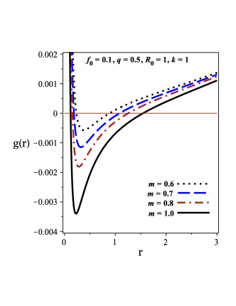
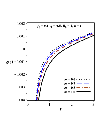
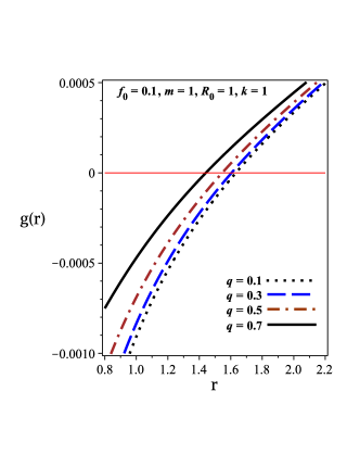
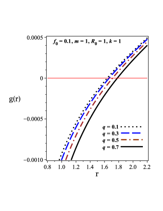
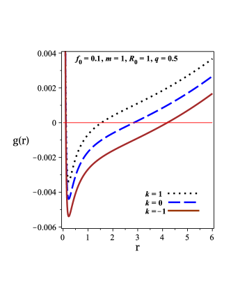
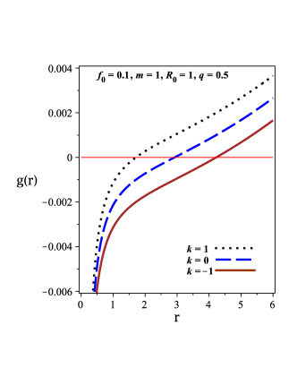
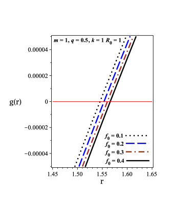
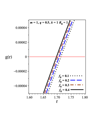
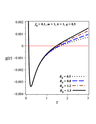
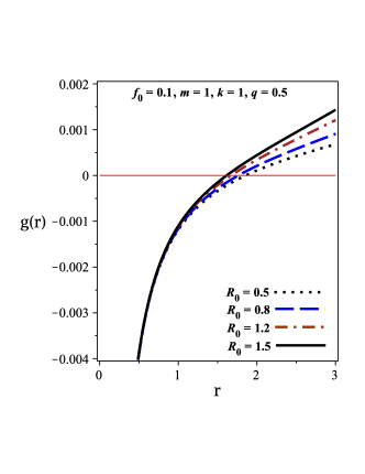
Figure 1: The metric function $g(r)$ versus $r$ for different values of the parameters. Left panels for $\eta=1$, and right panels for $\eta=-1$

III Thermodynamics

Now, we are going to calculate the conserved and thermodynamic quantities of the topological AdS phantom black hole solutions in $F(R)$ gravity to check the first law of thermodynamics.

For studying the thermodynamic properties of the obtained black hole solutions, it is necessary to express the mass ($m$) in terms of the radius of the event horizon $r_{+}$ and the charge $q$ as follows. Equating $g_{tt}=g(r)$ to zero, we have

$$m=\frac{kr_{+}}{2}+\frac{R_{0}r_{+}^{3}}{24}+\frac{\eta q^{2}}{2\left(1+f_{R_{0}}\right)r_{+}}.$$ (20)

Here, we want to obtain the Hawking temperature for these black holes. The superficial gravity of a black hole is given by

$$\kappa=\left.\frac{g_{tt}^{\prime}}{2\sqrt{-g_{tt}g_{rr}}}=\right|_{r=r_{+}}=\left.\frac{g^{\prime}(r)}{2}\right|_{r=r_{+}},$$ (21)

where $r_{+}$ is the radius of the events horizon. Considering the obtained metric function (16), and by substituting the mass (20) within the equation (21), one can calculate the superficial gravity as

$$\kappa=\frac{k}{2r_{+}}+\frac{R_{0}r_{+}}{8}-\frac{\eta q^{2}}{2\left(1+f_{R_{0}}\right)r_{+}^{3}},$$ (22)

and by using the Hawking temperature as $T=\frac{\kappa}{2\pi}$, we can extract it in the following form

$$T=\frac{k}{4\pi r_{+}}+\frac{R_{0}r_{+}}{16\pi}-\frac{\eta q^{2}}{4\pi\left(1+f_{R_{0}}\right)r_{+}^{3}}.$$ (23)

The electric charge of black hole per unit volume, $\mathcal{V}$, can be obtained by using the Gauss law as

$$Q=\frac{\widetilde{Q}}{\mathcal{V}}=\frac{F_{tr}}{4\pi}\int_{0}^{2\pi}\int_{0}^{\pi}\sqrt{g_{k}}d\theta d\varphi=\frac{q}{4\pi}$$ (24)

where $F_{tr}=\frac{q}{r^{2}}$, and for case $t=$ constant and $r=$constant, the determinant of metric tensor $g_{k}$ is $r^{4}\det\left(d\Omega_{k}^{2}\right)$ (i.e., $g_{k}=\det\left(g_{k}\right)=r^{4}\det\left(d\Omega_{k}^{2}\right)$). It is worthwhile to mention that in the above equation, we consider $\mathcal{V}=\int_{0}^{2\pi}\int_{0}^{\pi}\sqrt{\det\left(d\Omega_{k}^{2}\right)}d\theta d\varphi$, where it is the area of a unit volume of constant ($t$, $r$) space. Notable, $\mathcal{V}$ is $4\pi$ for $k=1$.

Considering $F_{\mu\nu}=\partial_{\mu}A_{\nu}-\partial_{\nu}A_{\mu}$, one can find the nonzero component of the gauge potential in which is $A_{t}=-\int F_{tr}dr$, and therefore the electric potential at the event horizon ($U$) with respect to the reference ($r\rightarrow\infty$) is given by

$$U=-\int_{r_{+}}^{+\infty}F_{tr}dr=\frac{q}{r_{+}}.$$ (25)

In order to obtain the entropy of black holes in $F(R)=R+f(R)$ theory, one can use a modification of the area law which means the Noether charge method Cognola2005

$$S=\frac{A(1+f_{R})}{4},$$ (26)

where $A$ is the horizon area and is defined

$$A=\left.\int_{0}^{2\pi}\int_{0}^{\pi}\sqrt{g_{\theta\theta}g_{\varphi\varphi}}\right|_{r=r_{+}}=\left.r^{2}\right|_{r=r_{+}}=r_{+}^{2},$$ (27)

so, the entropy of topological phantom AdS black holes per unit volume, $\mathcal{V}$, in $F(R)$ gravity is given by replacing the horizon area (27) within Eq. (26) as

$$S=\frac{\widetilde{S}}{\mathcal{V}}=\frac{(1+f_{R})r_{+}^{2}}{4},$$ (28)

which indicates that the area law does not hold for the black hole solutions in $R+f(R)$ gravity.

Using Ashtekar-Magnon-Das (AMD) approach AMDI ; AMDII , we find the total mass of these black holes per unit volume, $\mathcal{V}$, in $F(R)$ gravity as

$$M=\frac{\widetilde{M}}{\mathcal{V}}=\frac{m\left(1+f_{R}\right)}{4\pi},$$ (29)

where substituting the mass (20) within the equation (29), yields

$$M=\frac{\left(1+f_{R}\right)r_{+}}{2}\left(k+\frac{R_{0}r_{+}^{2}}{12}\right)+\frac{\eta q^{2}}{2r_{+}}.$$ (30)

It is straightforward to show that the conserved and thermodynamics quantities satisfy the first law of thermodynamics

$$dM=TdS+\eta UdQ,$$ (31)

where $T=\left(\frac{\partial M}{\partial S}\right)_{Q}$, and $\eta U=\left(\frac{\partial M}{\partial Q}\right)_{S}$, and they are in agreement with those of calculated in Eqs. (23) and (25), respectively.

IV Thermal Stability

Considering the black hole as a thermodynamic system, we want to study the local and global stability. In the following, we investigate the effects of the topological constant ($k$), the constant scalar curvature ($R_{0}$), and the parameter of $\eta$ on the local and global stability of the topological phantom (A)dS black holes in $F(R)$ gravity.

IV.1 Local Stability

Here, we would like to study the local stability of the topological phantom (A)dS black holes in the context of $F(R)$ gravity. For this purpose, by considering these black holes we will study the heat capacity and the geometrothemodynamics.

IV.1.1 Heat Capacity

In the canonical ensemble context, a thermodynamic system’s local stability can be studied by heat capacity. The heat capacity carries crucial information regarding the thermal structure of the black holes. This quantity includes three specific exciting pieces of information:

i) The discontinuities of heat capacity mark the possible thermal phase transitions that the system can undergo.

ii) The sign of it determines whether the system is thermally stable or not. In other words, the positivity corresponds to thermal stability while the opposite indicates instability.

iii) The roots of heat capacity are also of interest since they may yield the possible changes between stable/unstable states or bound points.

Due to these important points, we want to calculate the heat capacity of the solutions and investigation of local stability of the black holes by using such quantity.

Before obtaining the heat capacity, let us first re-write the total mass of the black hole (30) in terms of the entropy (28) in the following form

$$M\left(S,Q\right)=\frac{\pi^{2}Q^{2}\left(1+f_{R}\right)\eta+\frac{S\left(SR_{0}+3\left(1+f_{R}\right)k\right)}{12}}{\pi\sqrt{S\left(1+f_{R}\right)}},$$ (32)

using the equation (32), we re-write the temperature in the following form

$$T=\left(\frac{\partial M\left(S,Q\right)}{\partial S}\right)_{Q}=\frac{\frac{S\left(SR_{0}+\left(1+f_{R}\right)k\right)}{4}-\pi^{2}Q^{2}\left(1+f_{R}\right)\eta}{2\pi S^{3/2}\sqrt{1+f_{R}}}.$$ (33)

The heat capacity is defind as

$$C_{Q}=\frac{T}{\left(\frac{\partial T}{\partial S}\right)_{Q}}=\frac{\left(\frac{\partial M\left(S,Q\right)}{\partial\widetilde{S}}\right)_{Q}}{\left(\frac{\partial^{2}M\left(S,Q\right)}{\partial S^{2}}\right)_{Q}},$$ (34)

by considering Eqs. (32) and (33), we can obtain the heat capacity in form

$$C_{Q}=\frac{2S^{2}\left(\frac{SR_{0}}{\left(1+f_{R}\right)}+k\right)-8\pi^{2}Q^{2}S\eta}{12\pi^{2}Q^{2}\eta+S\left(\frac{SR_{0}}{\left(1+f_{R}\right)}-k\right)}.$$ (35)

In the context of black holes, it is argued that the root of heat capacity $\left(C_{Q}=T=0\right)$ is representing a border line between physical $\left(T>0\right)$ and non-physical $\left(T<0\right)$ black holes. We call it a physical limitation point. Indeed, the system in the case of this physical limitation point has a change in sign of the heat capacity. Also, it is believed that the divergences of the heat capacity represent phase transition critical points of black holes. So, the phase transition critical and limitation points of the black holes in the context of the heat capacity are calculated with the following relations

$$\left\{\begin{array}[]{ccc}T=\left(\frac{\partial M\left(S,Q\right)}{\partial S}\right)_{Q}=0,&&\text{physical limitation points}\\ &&\\ \left(\frac{\partial^{2}M\left(S,Q\right)}{\partial S^{2}}\right)_{Q}=0&&\text{phase transition critical points}\end{array}\right..$$ (36)

Using Eq. (33) and solving it in terms of the entropy, we can obtain physical limitation points as

$$\left\{\begin{array}[]{c}S_{root_{1}}=\frac{-\left(1+f_{R}\right)k}{2R_{0}}+\frac{\sqrt{\left[\left(1+f_{R}\right)k^{2}+16\pi^{2}Q^{2}\eta R_{0}\right]\left(1+f_{R}\right)}}{2R_{0}}\\ \\ S_{root_{2}}=\frac{-\left(1+f_{R}\right)k}{2R_{0}}-\frac{\sqrt{\left[\left(1+f_{R}\right)k^{2}+16\pi^{2}Q^{2}\eta R_{0}\right]\left(1+f_{R}\right)}}{2R_{0}}\end{array}\right..$$ (37)

To have the real root(s), we have to respect $\left(1+f_{R}\right)k^{2}+16\pi^{2}Q^{2}\eta R_{0}\geq 0$. This constraint gives us information about the effects of different parameters on the roots of temperature (33). For example, the temperature has one root for $k=0$, provided $\eta R_{0}>0$. For $k=\pm 1$, the temperature has two roots when $\eta R_{0}<0$, provided $R_{0}>\frac{-\left(1+f_{R}\right)k^{2}}{6\pi^{2}Q^{2}\eta}$. In addition, the relation $R_{0}>\frac{-\left(1+f_{R}\right)k^{2}}{6\pi^{2}Q^{2}\eta}$, imposes that for a large value of the electrical charge and $k=\pm 1$, the temperature does not have any root when the constant scalar curvature is negative. Indeed, the temperature of higher-charged black holes does not have any root when $k=\pm 1$ and $R_{0}<0$.

In order to study the phase transition critical points (or divergence points of the heat capacity), we have to solve the relation $\left(\frac{\partial^{2}M\left(S,Q\right)}{\partial S^{2}}\right)_{Q}=0$. So, we have

$$\left\{\begin{array}[]{c}S_{div_{1}}=\frac{\left(1+f_{R}\right)k}{2R_{0}}-\frac{\sqrt{\left[\left(1+f_{R}\right)k^{2}-48\pi^{2}Q^{2}\eta R_{0}\right]\left(1+f_{R}\right)}}{2R_{0}}\\ \\ S_{div_{2}}=\frac{\left(1+f_{R}\right)k}{2R_{0}}+\frac{\sqrt{\left[\left(1+f_{R}\right)k^{2}-48\pi^{2}Q^{2}\eta R_{0}\right]\left(1+f_{R}\right)}}{2R_{0}}\end{array}\right.,$$ (38)

where indicate that we have to respect $\left(1+f_{R}\right)k^{2}-48\pi^{2}Q^{2}\eta R_{0}\geq 0$, for having the real divergent point(s). Our analysis shows that the heat capacity has one divergent point for $k=0$, provided $\eta R_{0}<0$, and also there is no divergent point when $\eta R_{0}>0$. According to Eq. (38), for large values of the electrical charge, the heat capacity does not have any divergent point. In other words, the heat capacity of the higher-charged black holes does not have any divergent point. For $k=+1$ ( $k=-1$), the heat capacity has two divergence points when $\eta>0$ ($\eta<0$) and $R_{0}>0$ ($R_{0}<0$).

Now we can evaluate the local stability by using the behavior of temperature and heat capacity. For this purpose, we plot Fig. 2 and analyze them with more details in Table. 1.

Table 1: The local stability of the black holes for $Q=0.02$, $f_{R}=0.1$, and different values of $k$. First three rows are for $R_{0}=1$, and $\eta=1$. Second three rows are for $R_{0}=-1$, and $\eta=1$. Third three rows are for $R_{0}=1$, and $\eta=-1$. Fourth three rows are for $R_{0}=-1$, and $\eta=-1$.

$k$	number of $S_{root}$	number of $S_{div}$	physical area ($T>0$)	$C_{Q}>0$	local stability and physical area
$+1$	1	2	$S>S_{root}$	$\begin{array}[]{c}S_{root}<S<S_{div_{1}}\\ S>S_{div_{2}}\end{array}$	$\begin{array}[]{c}S_{root}<S<S_{div_{1}}\\ S>S_{div_{2}}\end{array}$
$0$	1	0	$S>S_{root}$	$S>S_{root}$	$S>S_{root}$
$-1$	1	0	$S>S_{root}$	$S>S_{root}$	$S>S_{root}$
$+1$	2	1	$S_{root_{1}}<S<S_{root_{2}}$	$\begin{array}[]{c}S_{root_{1}}<S<S_{div}\\ S>S_{root_{2}}\end{array}$	$S_{root_{1}}<S<S_{div}$
$0$	0	1	no area	$S>S_{div}$	no area
$-1$	0	1	no area	$S>S_{div}$	no area
$+1$	0	1	always positive	$S>S_{div}$	$S>S_{div}$
$0$	0	1	always positive	$S>S_{div}$	$S>S_{div}$
$-1$	2	1	$\begin{array}[]{c}S<S_{root_{1}}\\ S>S_{root_{2}}\end{array}$	$\begin{array}[]{c}S_{root_{1}}<S<S_{div}\\ S>S_{root_{2}}\end{array}$	$S>S_{root_{2}}$
$+1$	1	0	$S<S_{root}$	$S>S_{root}$	no area
$0$	1	0	$S<S_{root}$	$S>S_{root}$	no area
$-1$	1	2	$S<S_{root}$	$\begin{array}[]{c}S_{root}<S<S_{div_{1}}\\ S>S_{div_{2}}\end{array}$	no area

Our findings reveal some interesting behaviors which are:

i) The topological charged AdS black holes in $F(R)$ gravity satisfy the local stability condition when they have large radii (or large entropy), see the first three rows of Table. 1, for more details.

ii) The charged dS black holes with medium radii can be only locally stable for $k=1$ (see the second three rows of Table. 1, for more details).

iii) The phantom AdS large black holes have local stability (see the third three rows of Table. 1, for more details).

iv) There is no local stability area for the phantom AdS black holes with different topological constants (see the fourth three rows in Table. 1, for more details).

We plotted the figure. 2, for more details. Two up panels in Fig. 2 belong to the charged (A)dS black holes in $F(R)$ gravity for $k=+1$ and $k=-1$. Also, the two down panels are related to phantom (A)dS black holes in $F(R)$ gravity for $k=+1$ and $k=-1$. In Fig. 2, the hatched areas belong to the physical and local stability of these black holes.

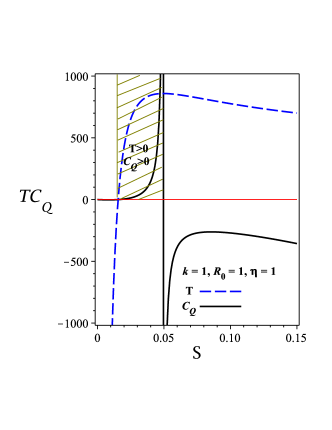
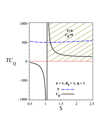
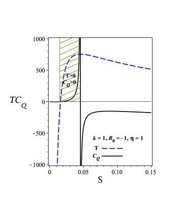
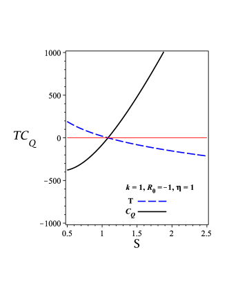
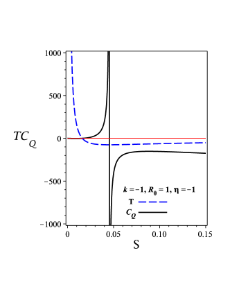
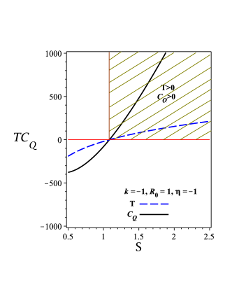
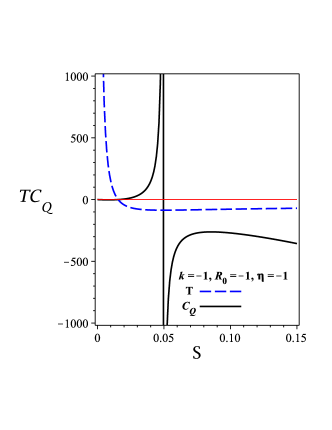
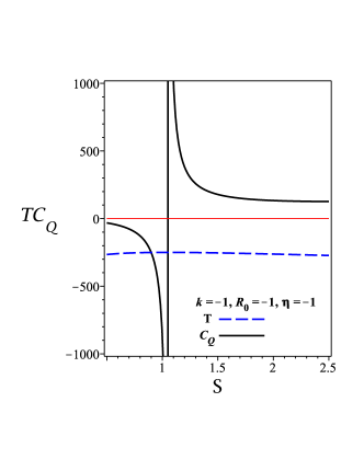
Figure 2: The heat capacity ($C_{Q}$) and temperature ($T$) versus $S$ for $Q=0.02$ and $f_{R}=0.1$. We plot them in different scales in order to be more clear.

IV.1.2 Geometrothermodynamics

Here, we want to study the phase transition of the topological phantom (A)dS black holes in $F(R)$ gravity through geometrothemodynamics. In the geometrothemodynamics method, a thermodynamical metric (thermodynamical phase space) is constructed by considering one of the thermodynamical quantities as thermodynamical potential and other quantities as extensive parameters. By calculating the Ricci scalar of such a thermodynamical metric and determining its divergence point(s), one can obtain the phase transition point(s) of the system. In this regard, several thermodynamical metrics have been introduced in order to build a geometrical phase space by thermodynamical quantities. The famous ones are the Weinhold Weinhold1 ; Weinhold2 , Ruppeiner Ruppeiner1 ; Ruppeiner2 , and Quevedo metrics Quevedo1 ; Quevedo2 . It was previously argued that these metrics may not provide us with a completely flawless mechanism for evaluating the geometrothemodynamics of specific types of black holes (see Refs. HPEM1 ; HPEM2 ; HPEM3 ; HPEM4 ; HPEM5 ; HPEM6 , for more details). Recently, a new metric (which is known as HPEM metric HPEM1 ), was introduced in order to solve the problems that other metrics may confront with it. In this section, we would like to investigate the phase transition of the topological phantom (A)dS black holes in the non-extended phase space via the geometrothemodynamics method which is described by the HPEM metric.

The HPEM metric is given by HPEM1

$$ds^{2}=\frac{SM_{S}}{M_{QQ}^{3}}\left(-M_{SS}dS^{2}+M_{QQ}dQ^{2}\right),$$ (39)

where $M_{S}=\frac{\partial M}{\partial S}$, $M_{SS}=\frac{\partial^{2}M}{\partial S\partial S}$, and $M_{QQ}=\frac{\partial^{2}M}{\partial Q\partial Q}$. Since we are looking for the divergence points of the HPEM’s Ricci scalar and because its numerator is a smooth finite function, we focus on the denominator of the HPEM’s Ricci scalar. The denominator of the HPEM’s Ricci scalar is given by HPEM1

$$denom(R)=2S^{3}M_{S}^{3}M_{SS}^{2}.$$ (40)

To have a proper geometrothemodynamics approach for studying phase transitions, the thermodynamic Ricci scalar should diverge at points which we mentioned before with bound $\left(M=\frac{\partial M}{\partial S}=0\right)$ and phase transition $\left(M_{SS}=\frac{\partial^{2}M}{\partial S^{2}}=0\right)$ points (see Eq. (36), for more details). Regarding Eq. (40), it is evident that the divergence points and root of the heat capacity coincide with divergences of the HPEM’s Ricci scalar. In other words, the denominator of the Ricci scalar of the HPEM metric contains the numerator and denominator of the heat capacity (Eq. (34)). Indeed the divergence points of the Ricci scalar of the HPEM metric coincide with both roots and phase transition critical points of the heat capacity. So, all the physical limitations and the phase transition critical points are included in the divergences of the Ricci scalar of the HPEM metric (see Fig. 3, for more detail). As a result, the HPEM metric provides a successful mechanism for investigating the bound and phase transition points of such black holes.

Looking at the figure. 3, we can find another important behavior of the HPEM metric which is related to the different behavior of the Ricci scalar before and after its divergence points. The behavior of HPEM’s Ricci scalar for divergence points related to the physical limitation and phase transition critical points is different. In other words, the sign of HPEM’s Ricci scalar changes before and after divergencies when the heat capacity is zero. However, the signs of the Ricci scalar are the same when the heat capacity encounters with divergences. These divergences are called $\Lambda$ divergences. Therefore, considering this approach also enable us to distinguish the physical limitation and the phase transition critical points from one another (see Fig. 3, for more details).

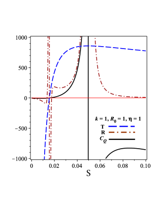
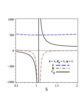
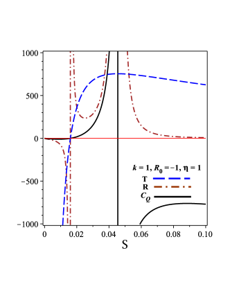
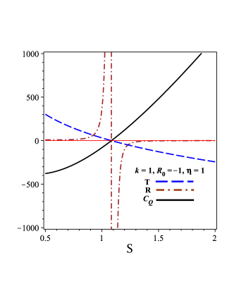
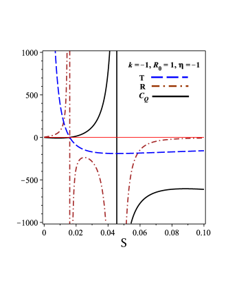
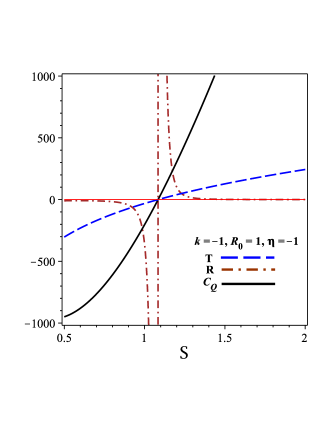
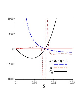
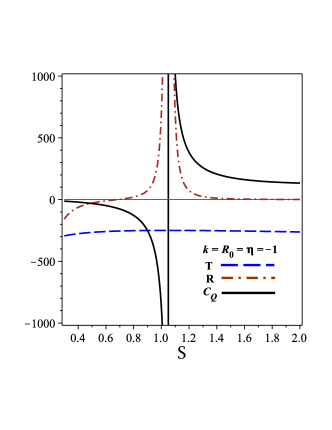
Figure 3: The heat capacity ($C_{Q}$) and temperature ($T$) and Ricci scalar ($R$) versus $S$ for $Q=0.02$ and $f_{R}=0.1$. We plot them in different scales to be more clear.

IV.2 Global Stability

In the context of the grand-canonical ensemble, the global stability of a thermodynamic system can be studied by Gibbs’s potential. In other words, the negative of the Gibbs potential determines the global stability of a thermodynamic system. On the other hand, the negative of the Helmholtz free energy of a thermodynamic system satisfies the global stability in the context of the canonical ensemble. Therefore, by using the Gibbs potential and the Helmholtz free energy, we want to evaluate the global stability of the topological phantom (A)dS black holes in $F(R)$ gravity.

IV.2.1 Gibbs Potential

The Gibbs potential is defined in the following form

$$G=M\left(S,Q\right)-TS-\eta UQ,$$ (41)

by using the relation $\eta U=\left(\frac{\partial M}{\partial Q}\right)_{S}$ and Eqs. (32) and (33), we get the Gibbs potential as

$$G=\frac{\frac{S}{12}\left(3\left(1+f_{R}\right)k-SR_{0}\right)-\pi^{2}Q^{2}\left(1+f_{R}\right)\eta}{2\pi\sqrt{S\left(1+f_{R}\right)}},$$ (42)

where the roots of the Gibbs potential are given by

$$\left\{\begin{array}[]{c}S_{G_{1}}=\frac{3\left(1+f_{R}\right)k}{2R_{0}}-\frac{\sqrt{3\left[3\left(1+f_{R}\right)k^{2}-16\pi^{2}Q^{2}\eta R_{0}\right]\left(1+f_{R}\right)}}{2R_{0}}\\ \\ S_{G_{2}}=\frac{3\left(1+f_{R}\right)k}{2R_{0}}+\frac{\sqrt{3\left[3\left(1+f_{R}\right)k^{2}-16\pi^{2}Q^{2}\eta R_{0}\right]\left(1+f_{R}\right)}}{2R_{0}}\end{array}\right..$$ (43)

In order to study global stability, we must consider $G<0$. In other words, the black holes have a global stable when $G<0$. To evaluate the global stability of the topological phantom (A)dS black holes in $F(R)$ gravity, we plotted four panels in Fig. 4 (see the panels ($4a$), ($4b$), ($4c$), and ($4d$) in Fig. 4). Our analysis reveals some results which are:

i) The charged AdS black holes with $k=0$, and $k=-1$ are stable everywhere (i.e., $S\in\left(0,+\infty\right)$). For $k=1$, the global stability is located in the range $S\in\left(0,S_{G_{1}}\right)\cup\left(S_{G_{2}},+\infty\right)$, see the panel ($4a$) in Fig. 4.

ii) The charged dS black holes with small radii and different topological constants have global stability. In other words, the Gibbs potential is negative for $S<S_{G}$ (see the panel ($4b$) in Fig. 4).

iii) The phantom AdS black holes in $F(R)$ gravity with large radii and different topological constants are stable because the Gibbs potential is negative for $S>S_{G}$ (see the panel ($4c$) in Fig. 4).

iv) Whereas the Gibbs potential is negative in the range $S\in\left(0,S_{G_{1}}\right)\cup\left(S_{G_{2}},+\infty\right)$ for the phantom dS black holes in $F(R)$ gravity with $k=-1$. In other words, these black holes are stable in these areas (i.e., $S\in\left(0,S_{G_{1}}\right)\cup\left(S_{G_{2}},+\infty\right)$), see the panel ($4d$) in Fig. 4.

IV.2.2 Helmholtz Free Energy

Another mechanism for determining the global stability of a thermodynamic system is related to the Helmholtz free energy. It is notable that in the usual case of thermodynamics the Helmholtz free energy is given by $F=U-TS$. However, in the context of the black holes, Helmholtz free energy is defined in the following form

$$F(T,Q)=M\left(S,Q\right)-TS,$$ (44)

where by considering Eqs. (32) and (33), we can obtain the Helmholtz free energy as

$$F(T,Q)=\frac{3\pi^{2}Q^{2}\left(1+f_{R}\right)\eta-\frac{S}{12}\left(SR_{0}-3\left(1+f_{R}\right)k\right)}{2\pi\sqrt{S\left(1+f_{R}\right)}},$$ (45)

and by solving $F(T,Q)=0$, we get the roots of the Helmholtz free energy that are

$$\left\{\begin{array}[]{c}S_{F_{1}}=\frac{3\left(1+f_{R}\right)k}{2R_{0}}-\frac{3\sqrt{\left[\left(1+f_{R}\right)k^{2}+16\pi^{2}Q^{2}\eta R_{0}\right]\left(1+f_{R}\right)}}{2R_{0}}\\ \\ S_{F_{2}}=\frac{3\left(1+f_{R}\right)k}{2R_{0}}+\frac{3\sqrt{\left[\left(1+f_{R}\right)k^{2}+16\pi^{2}Q^{2}\eta R_{0}\right]\left(1+f_{R}\right)}}{2R_{0}}\end{array}\right..$$ (46)

The global stability areas are given when the Helmholtz free energy is negative (i.e., $F<0$). To evaluate the global stability of the topological phantom (A)dS black hole in $F(R)$ gravity, we plot the Helmholtz free versus $S$ in Fig. 4. Our results are:

i) The charged AdS black holes with different topological constants are stable when $S>S_{F_{2}}$. Indeed, the large black holes have global stability (see the panel ($4e$) in Fig. 4).

ii) There are only stable areas for the charged dS black holes with $k=-1$ when the entropy is located between two roots (i.e., $S_{F_{1}}<S<S_{F_{2}}$), see the panel ($4f$) in Fig. 4.

iii) The phantom AdS black holes with $k=0$, and $k=-1$ are stable. Whereas for $k=1$, the global stability areas are located in the range $S\in\left(0,S_{G_{1}}\right)\cup\left(S_{G_{2}},+\infty\right)$, see the panel ($4g$) in Fig. 4.

iv) The phantom dS black holes with different topological constants and small radii are stable (see the panel ($4h$) in Fig. 4).

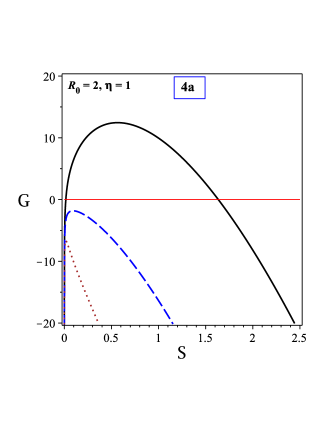
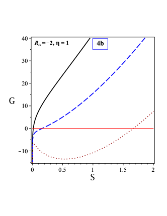
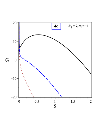
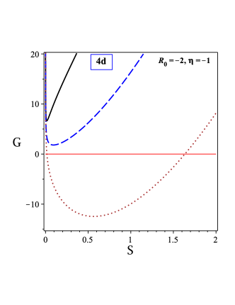
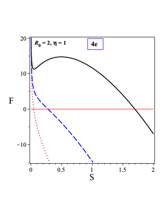
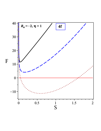
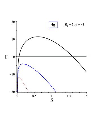
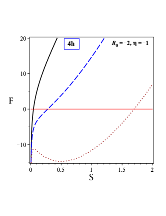
Figure 4: $G$ (and $F$) versus $S$ for $Q=0.02$, and $f_{R}=0.1$. Also, $k=1$ (continuous line), $k=0$ (dashed line), and $k=-1$ (dotted line).

In order to have more details of the global stability from two points of view, we plot the Gibbs potential and the Helmholtz free energy together versus the entropy in Fig. (5).

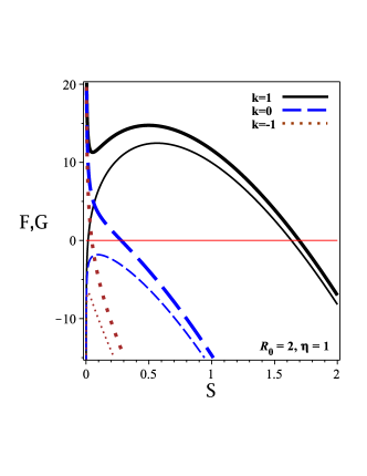
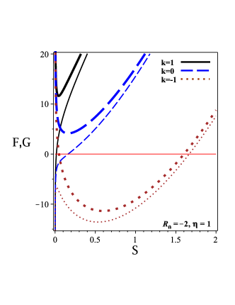
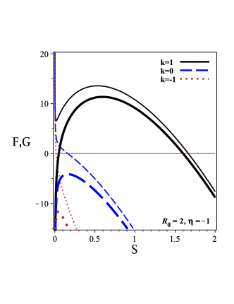
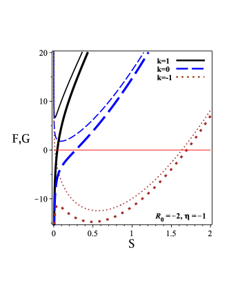
Figure 5: The Gibbs potential and the Helmholtz free energy versus $S$ for $Q=0.02$, and $f_{R}=0.1$. Thin and bold lines are related to $G$ and $F$, respectively.

Comparing these points of view, we find some different behaviors of the global stability for black holes in $F(R)$ gravity. These results are:

i) Generally, by considering the charged AdS black holes with different topological constants, the Gibbs potential covers a large global stability area compared with the Helmholtz free energy. There is the same behavior for the charged AdS black holes with large radii. Indeed, the large black holes with $k=0$, $\pm 1$ in two points of view are stable. However, considering the Gibbs potential, the small charged AdS black holes are stable. Using the two points of view, the charged AdS black holes with different topological constants and large radii are always stable (see the left-up panel in Fig. 5, for more details).

ii) Using the Gibbs potential, the charged dS black holes with small radii and different topological constants are always stable, whereas there is no stable area for small black holes in the viewpoint of the Helmholtz free energy. In addition, from point of view of Helmholtz free energy, the charged dS black holes with medium radii can be stable when $k=-1$. As a common result from both viewpoints, the charged dS black holes with large radii and $k=0$, $\pm 1$ do not have the global stability area (see the right-up panel in Fig. 5, for more details).

iii) In total, the Helmholtz free energy covers a large global stability area compared with the Gibbs potential for the phantom AdS black holes with different topological constants. Our findings indicate that the phantom AdS black holes with large radii are always stable in the two points of view. On the other hand, small phantom AdS black holes are only stable in the viewpoint of the Helmholtz free energy (see the left down panel in Fig. 5, for more details).

iv) The phantom dS black holes with small radii can be always stable in the viewpoint of Helmholtz free energy. However, from point of view of Gibbs’s potential, the phantom dS black holes with medium radii can be only stable when $k=-1$ (see the right down panel in Fig. 5, for more details).

V Conclusions

In section II, we obtain an exact solution of the case of the theory $F(R)$ with constant curvature, for a topological metric in four dimensions, coupling a spin$-1$ phantom field. We show this solution has one or two horizons, depending on the value of the topological constant $k$, the mass, the charge, the coupling constant $\eta$, and the scalar $R_{0}$.

In section III, we define the temperature, electric field, and entropy of the solution, as well as establish the first law of thermodynamics, showing that the term related to thermodynamic work can be positive or negative, depending on whether the field is phantom or not. This property was already known in phantom solutions manuel1 .

In section IV, we first study local thermodynamic stability, through the zeros and divergent points of the heat capacity, as well as the geometrothemodynamics, agreeing between the two approaches. Then we study global thermodynamic stability by analyzing the sign of the Gibbs potential and Helmholtz free energy. In general, the two approaches agree on slightly different ranges of entropy.

We should also analyze, in a future work, the geodesics of this solution, as well as the shadow and stability, checking the absorption and scattering of scalar fields.

We can find astrophysical evidence of the signature of the phantom modification of the electromagnetic contribution in the following situations:

a) the shadow of this black hole must present characteristics of differentiation between the usual Reissner-Nordström one, thus being able to serve as experimental evidence.

b) the new phantom signature must also appear in the gravitational wave ringdown of this solution.

c) observational evidence can also be obtained through gravitational lensing phenomena.

- (1) S. Perlmutter et al., Astrophys. J. 517, 565 (1999);
- (2) A. G. Riess et al., Astrophys. J. 607, 665 (2004).
- (3) D. N. Spergel et al., Astrophys. J. Suppl. 170, 377 (2007).
- (4) S. Cole et al., Mon. Not. Roy. Astron. Soc. 362, 505 (2005).
- (5) H. A. Buchdahl, Mon. Not. Roy. Astron. Soc. 150, 1 (1970).
- (6) S. M. Carroll, V. Duvvuri, M. Trodden, and M. S. Turner, Phys. Rev. D 70, 043528 (2004).
- (7) T. P. Sotiriou and V. Faraoni, Rev. Mod. Phys. 82, 451 (2010).
- (8) S. Nojiri, S. D. Odintsov, and V. K. Oikonomou, Phys. Rept. 692, 1 (2017).
- (9) A. A. Starobinsky, Phys. Lett. B 91, 99 (1980).
- (10) I. Sawicki, and W. Hu, Phys. Rev. D 75, 127502 (2007).
- (11) L. Amendola, and S. Tsujikawa, Phys. Lett. B 660, 125 (2008).
- (12) S. Tsujikawa, Phys. Rev. D 77, 023507 (2008).
- (13) G. Cognola, E. Elizalde, S. Nojiri, S. D. Odintsov, L. Sebastiani, and S. Zerbini, Phys. Rev. D 77, 046009 (2008).
- (14) S. Capozziello, E. Piedipalumbo, C. Rubano, and P. Scudellaro, Astron. Astrophys. 505, 21 (2009).
- (15) A. V. Astashenok, S. Capozziello, and S. D. Odintsov, JCAP 12, 040 (2013).
- (16) S. Capozziello, and A. Troisi, Phys. Rev. D 72, 044022 (2005).
- (17) S. Capozziello, A. Stabile, and A. Troisi, Phys. Rev. D 76, 104019 (2007).
- (18) P. J. E. Peebles and Bharat Ratra, Rev. Mod. Phys. 75, 559 (2003).
- (19) Z. K. Guo, Y. S. Piao, X. Zhang and Y. Z. Zhang. Physics Letters B, 608, 177 (2005).
- (20) A. de la Cruz-Dombriz, A. Dobado, and A. L. Maroto, Phys. Rev. D 80, 124011 (2009).
- (21) T. Moon, Y. S. Myung, and E. J. Son, Gen. Relativ. Gravit 43, 3079 (2011).
- (22) S. H. Hendi, B. Eslam Panah, and S. M. Mousavi, Gen. Relativ. Gravit. 44, 835 (2012).
- (23) S. H. Mazharimousavi, and M. Halilsoy, Phys. Rev. D 84, 064032 (2011).
- (24) D. Bazeia, L. Losano, Gonzalo J. Olmo, and D. Rubiera-Garcia, Phys. Rev. D 90, 044011 (2014).
- (25) M. E. Rodrigues, E. L. B. Junior, G. T. Marques, and V. T. Zanchin, Phys. Rev. D 94, 024062 (2016).
- (26) A. K. Mishra, M. Rahman, and S. Sarkar, Class. Quantum Grav. 35, 145011 (2018).
- (27) G. G. L. Nashed, and S. Capozziello, Phys. Rev. D 99, 104018 (2019).
- (28) M. Zhang, and R. B. Mann, Phys. Rev. D 100, 084061 (2019).
- (29) G. G. L. Nashed, and E. N. Saridakis, Phys. Rev. D 102, 124072 (2020).
- (30) B. Eslam Panah, J. Math. Phys. 63, 112502 (2022).
- (31) M. E. Rodrigues, E. L. B. Junior, G. T. Marques, and Julio C. Fabris, Eur. Phys. J. C 76, 250 (2016).
- (32) A Einstein, N Rosen, Phys. Rev. 48: 73 (1935).
- (33) M. Visser, Lorentzian Wormholes: from Einstein to Hawking. Springer-Verlag, New York (1996),
- (34) G. Clement, J. C. Fabris and M. E. Rodrigues, Phys. Rev. D 79, 064021 (2009).
- (35) K. A. Bronnikov and J. C. Fabris, Phys. Rev. Lett. 96, 251101 (2006).
- (36) M. Azreg-Ainou, G. Clement, J. C. Fabris and M. E. Rodrigues, Phys. Rev. D 83, 124001 (2011).
- (37) D. F. Jardim, M. E. Rodrigues and S. J. M. Houndjo, Eur. Phys. J. Plus 1270: 123 (2012).
- (38) G. Cognola, E. Elizalde, S. Nojiri, S. D. Odintsov and S. Zerbini, JCAP 02, 010 (2005).
- (39) A. Ashtekar, and A. Magnon, Class. Quantum Gravit. 1, L39 (1984).
- (40) A. Ashtekar, and S. Das, Class. Quantum Gravit. 17, L17 (2000).
- (41) F. Weinhold, J. Chem. Phys. 63, 2479 (1075).
- (42) F. Weinhold, J. Chem. Phys. 63, 2484 (1975).
- (43) G. Ruppeiner, Phys. Rev. A 20, 1608 (1979).
- (44) G. Ruppeiner, Rev. Mod. Phys. 67, 605 (1995).
- (45) H. Quevedo, Gen. Relativ. Gravit. 40, 971 (2008).
- (46) H. Quevedo, A. Sanchez, S. Taj, and A. Vazquez, Gen. Relativ. Gravit. 43, 1153 (2011).
- (47) S. H. Hendi, S. Panahiyan, B. Eslam Panah, and M. Momennia, Eur. Phys. J. C 75, 507 (2015).
- (48) S. H. Hendi, S. Panahiyan, and B. Eslam Panah, Adv. High Energy Phys. 2015, 743086 (2015).
- (49) S. H. Hendi, A. Sheykhi, S. Panahiyan, and B. Eslam Panah, Phys. Rev. D 92, 064028 (2015).
- (50) S. H. Hendi, B. Eslam Panah, and S. Panahiyan, JHEP 05, 029 (2016).
- (51) B. Eslam Panah, Phys. Lett. B 787, 45 (2018).
- (52) Kh. Jafarzade, J. Sadeghi, B. Eslam Panah, and S. H. Hendi, Ann. Phys. 432, 168577 (2021).
- (53) M. E. Rodrigues and Z. A.A. Oporto, Phys. Rev. D 85: 104022 (2012).