Granular-ball Optimization Algorithm

Abstract

The existing intelligent optimization algorithms are designed based on the finest granularity, i.e., a point. This leads to weak global search ability and inefficiency. To address this problem, we proposed a novel multi-granularity optimization algorithm, namely granular-ball optimization algorithm (GBO), by introducing granular-ball computing. GBO uses many granular-balls to cover the solution space. Quite a lot of small and fine-grained granular-balls are used to depict the important parts, and a little number of large and coarse-grained granular-balls are used to depict the inessential parts. Fine multi-granularity data description ability results in a higher global search capability and faster convergence speed. In comparison with the most popular and state-of-the-art algorithms, the experiments on twenty benchmark functions demonstrate its better performance. The faster speed, higher approximation ability of optimal solution, no hyper-parameters, and simpler design of GBO make it an all-around replacement of most of the existing popular intelligent optimization algorithms.

1 Introduction

In the field of scientific research and engineering, we often need to calculate the global optimal solution of functions, including unimodal and multi-modal functions. Hussien et al. (2020); Rashedi et al. (2018); Huband et al. (2006); Weile and Michielssen (1997). Multi-modal functions are more difficult, it is easy to fall into local optimal solution and the calculation cost is high. To solve these problems, researchers have put forward a lot of solutions.

In order to avoid falling into a local optimal solution as much as possible, Bergh et al. designed a cooperative particle swarm optimization (CPSO) Van den Bergh and Engelbrecht (2004), which uses multiple populations to work together and shares information. Yang et al. Yang et al. (2016) proposed an adaptive continuous ant colony optimization algorithm, which uses a local search strategy based on Gaussian distribution. It provides a good balance between the global and local, and will not fall into the local optimal solution prematurely. Zhang et al. proposed an adaptive particle swarm optimization (IDPSO) Zhang et al. (2013), which dynamically set the evolution direction of each particle by adjusting three parameters. Zhang et al. Zhang et al. (2020) proposed a particle swarm optimization algorithm based on dynamic neighborhood. It use a dynamic neighborhood selection mechanism to determine the position update direction of particles. It is better balance the relationship between global exploration and local exploitation. Wang et al. Wang et al. (2013) used an adaptive mutation strategy to help the captured particles escape from the local optimal solutions, which can improve the mutation performance of PSO effectively. Qu et al.Qu et al. (2012) designed a new local search technique, which improves the probability of finding the global optimal solution.

To reduce the computational cost, Song et al. improved the three components of individual selection, population diversity, and adaptive parameters in the particle swarm optimization algorithm Song et al. (2019). Different particles performs different search tasks, and they shares information. Zhou et al. proposed a bee algorithm Zhou et al. (2016) used a local search method to speed up the local search. It showed faster computational speed and higher computational accuracy in computing multi-modal functions. Cheng et al. Cheng et al. (2017) designed an adaptive peak detection method. First, they find out the peaks where the optimal solution may exist. Then, they do a fine search in this region and a coarse search in other regions. The method can reduce unnecessary computations in some regions. Li et al.Li et al. (2020) proposed a multi-modal whale optimization algorithm. They used localization and Gaussian sampling to improve searchability. Li et al. Li and Tan (2017) designed a competition-based fireworks algorithm. It uses competition as an interactive way and compares fireworks according to their current status and progress, continuously eliminating the losers. This method greatly improves the computational efficiency of multi-modal functions.

Our world is displayed in a multi-granularity way. From the perspective of granular computing or granular computing Xia et al. (2019); Wang (2017), the existing intelligent optimization algorithms are optimized based on the most fine-grained points, so they do not have the efficiency and global characterization ability of multi-granularity. To this end, we propose a novel optimization algorithm inspired by granular-ball computing. The main contributions of the paper are as follows:

• We propose a multi-granularity optimization algorithm GBO which can simulate the multi-granularity distribution of data. Different from the existing intelligence optimization algorithms, its optimization process is based on granular-balls with different sizes, rather than sampling points. This leads to better convergence performance than other algorithms.

• In GBO, the unimportant part of the solution space is covered by a small amount of coarse-grained granular-balls, which makes GBO avoid a large number of search calculations. So, it has a faster convergence speed than the existing intelligent optimization algorithms.

• In GBO, the important part of the solution space is covered by a large amount of fine-grained granular-balls, which makes GBO have better search ability of the optimal solution than the existing intelligent optimization algorithms.

• GBO contains no hyper-parameters. So, GBO is completely adaptive, which is a characteristics that the existing intelligence optimization algorithms do not have. Not relying on any hyper-parameters also lead to higher stability than the existing algorithms.

• GBO is very simple, and easy to be implemented.

The rest of this paper is organized as follows: we introduce related works in Section 2. Section 3 introduces the structure and details of granular-ball optimization algorithm. Experimental results and analysis are provided in Section 4. We conclude the whole work and discuss the future work in Section 5.

2 Related Work about Granular-ball Computing

In 1982, Chen Chen (1982) pointed out that the brain gives priority to recognizing a “wide range” of contour information in image recognition, and human cognition has the characteristics of “global precedence”. It is different from the major existing artificial intelligence algorithms, which take the most fine-grained points as input. The human brain’s global precedence cognition is efficient and robust, and is very beneficial for improving the performance of the existing artificial intelligence algorithms. Wang Wang (2017) first introduced the large-scale cognitive rule into granular computing and proposed multi-granular cognitive computing. Xia and Wang Xia et al. (2020, 2022c, 2022a) further used hyperspheres of different sizes to represent ”grains”, and proposed granular-ball computing, in which a large granular-ball represents coarse granularity, while a small granular-ball represents fine granularity. Granular-ball computing was initially used to deal with classification problems successfully. A schematic diagram of appling granular-ball computing into classification problems is shown in Fig. 1.

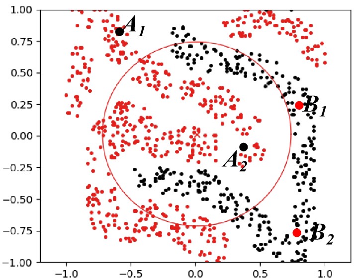
(a)

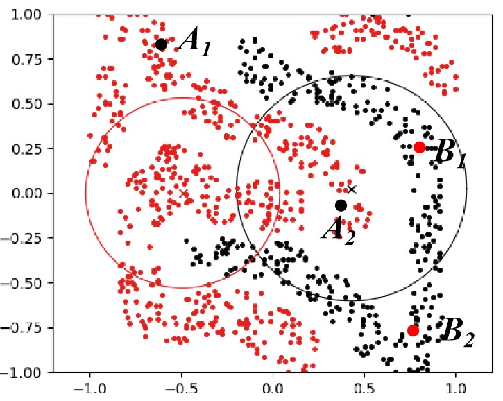
(b)

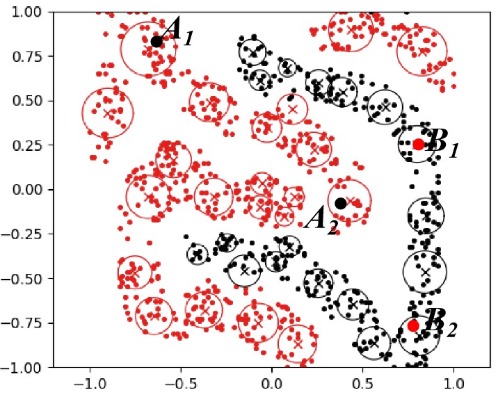
(c)

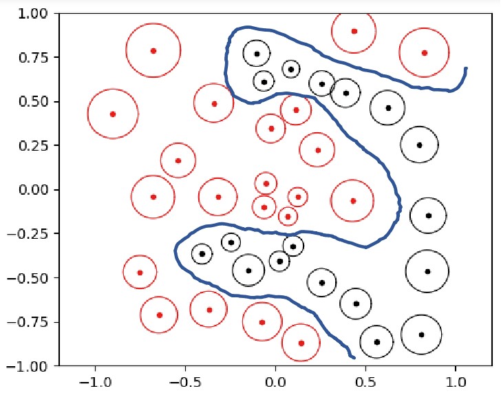
(d)

Figure 1: The granular-ball splitting generation process. $A_{1}$, $A_{2}$, $B_{1}$, and $B_{2}$ are noise points.

As shown in Fig. 1, the granular-ball in Fig. 1(1(a)) is the coarsest one. At this time, its quality of is not high and continues to split into two fine granular-balls(as shown in Fig. 1(1(b))). At this point, the quality of the granular-ball still cannot meet the requirements, and it will continue to split until the splitting process converges (as shown in Fig. 1(1(c)). Fig. 1(1(d)) is the result after the data is transformed into granular-balls, and the blue is the decision curve obtained after the training and learning of granular-balls. Since the four fine-grained noise points in Fig. 1(1(c)) do not affect the label of the coarse-grained granular-ball, the learning process based on granular-ball is robust. As the number of granular-balls in Fig. 1(1(d)) is far less than the number of samples in Fig. 1(1(a)), the learning based on granular-ball is efficient. The generation model of granular-ball is as follows.

Given a data set $D={x_{i}(i=1,2,\dots,n)}$, where $n$ is the number of samples on $D$. Granular balls $GB_{1},GB_{2},\dots,GB_{m}$ are used to cover and represent the data set $D$. Suppose the number of samples in the $j^{th}$ granular-ball $GB_{j}$ is expressed as $|GB_{j}|$, then its coverage degree can be expressed as ${\textstyle\sum_{i=1}^{m}}\left(\left|GB_{j}\right|\right)/n$. The basic model of granular-ball coverage can be expressed as

$$\begin{split}min\ \ \lambda_{1}\ast n/{\sum_{j=1}^{m}}\left(\left|GB_{j}\right|\right)/n+\lambda_{2}\ast m,\\ s.t.\ \ quality(GB_{j})\geq T,\ \ \ \ \ \ \ \ \ \ \ \ \ \ \ \ \ \ \ \ \ \ \ \ \end{split}$$ (1)

where $\lambda_{1}$ and $\lambda_{2}$ are the corresponding weight coefficients, and $m$ the number of granular balls. When other factors remain unchanged, the higher the coverage, the less the sample information is lost, and the more the number of granular-balls, the the characterization is more accurate. Therefore, the minimum number of granular-balls should be considered to obtain the maximum coverage degree when generating granular-balls. By adjusting the parameters $\lambda_{1}$ and $\lambda_{2}$, the optimal granular-ball generation results can be obtained to minimize the value of the whole equation. In most cases, the two items in the objective function do not affect each other and do not need trade off, so $\lambda_{1}$ and $\lambda_{2}$ are set to 1 by default. Granular-ball computing can fit arbitrarily distributed data Xia et al. (2019, 2022c).

Shuyin Xia and Guoyin Wang et al. proposed the GBSVM method Xia et al. (2019, 2022c). There is no the finest granularity point $x_{i}$ in GBSVM, and $x_{i}$ is replaced with a granular-ball with a center $c_{i}$ and radius $r_{i}$. A large $r_{i}$ represents a coarse granularity, and a smaller value represents a fine granularity. GBSVM is the first multi-granularity classifier model that is not based on point-input (i.e., containing $x_{i}$), and exhibits better efficiency and robustness than the traditional classifier at the same time. Granulular-ball computing is also applied into many other learning methods to improve their generalizability or efficiency, such as rough sets Shuyin et al. (2022), sampling for classification Xia et al. (2021), fuzzy sets Xia et al. (2022b), and so on. In this paper, we want to propose a multi-granularity optimization algorithm based on the idea of granular computing, and make it have the multi-granularity global optimization ability and high performance in efficiency.

3 Method

3.1 Motivation

The comparison between traditional intelligent optimization algorithms and GBO is shown in Fig. 2. As shown in Fig. 2(2(a)), the existing intelligent optimization algorithms are designed based on the finest granularity, i.e., point samples. By continuously generating new samples, the objective function value of the optimal sample is constantly close to the optimal solution. In the minimum optimization problem, the value of the minimum sample function is decreasing. The whole process is based on the calculation of the most fine-grained samples. In contrast, granular-ball optimization is based on coarse-grained and multi-grained. The same number of granular-balls can better describe and cover the solution space. Therefore, in comparison with those traditional optimization algorithms based on the most fine-grained sample, it can obtain higher convergence speed and approximation ability of the optimal solution.

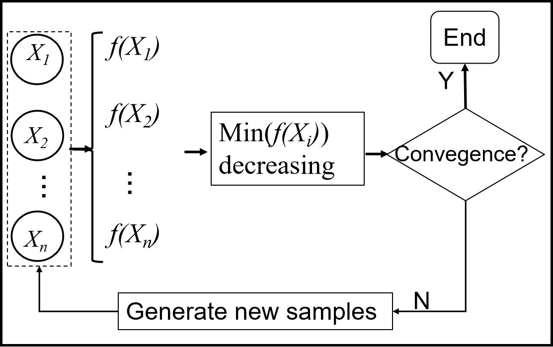
(a)

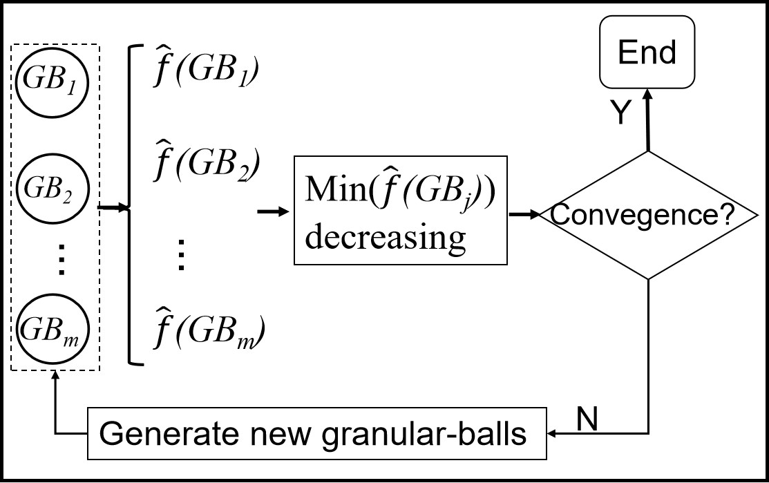
(b)

Figure 2: Comparison between traditional intelligent optimization algorithms and GBO in a minimum optimization problem. (2(a)) $X_{i}$ and $f(X_{i}),i=1,2,\dots,n$ denote a sampled point and its function value. (2(b)) GBO based on coarse granularity. $GB_{j}$ and $\hat{f}(GB_{j}),j=1,2,\dots,m$ denote a granular-ball and its function value.

In order to simulate the global precedence characteristics of human cognition at the beginning of the algorithm. As the process decribed in Fig. 1. First, we use a granular-ball to cover the whole solution space of the function. Then, with the idea from coarse-grained to fine-grained, the granular-balls are split. In granular-ball computing, the larger the granular-ball, the higher the efficiency, but it is more likely to lead to the neglect of details and the loss of precision. The smaller the granular-ball, the more times repeated calculation will reduce the efficiency. Therefore, the whole process involves three research issues including how to represents a granular-ball, how to measure the quality of each granular-ball, and how to design the splitting strategy of granular-ball.

3.2 GBO algorithm Framework

Aiming at dealing with three above problems involved in GBO, we firstly designed the quality evaluation method of a granular-ball.

3.2.1 Quality Evaluation of a Granular-ball

Our goal is to search the global minimum of the function, so the smaller the objective function value of a granular-ball, the higher its quality. Assuming that the center of the granular-ball is the origin of the coordinate axis, and the intersection points between the granular-ball and the coordinate axis are boundary points. A granular-ball can be represented using its boundary points Xia et al. (2021), which can be expressed in a parsed way. The optimal value of a granular-ball is the minimum function value of all the boundary points. The objective function value of a granular-ball is defined as follows.

Definition 1.

Given a granular-ball $GB$, its radius and center are $r$ and $c=[c_{1},c_{2},\dots,c_{d}]$, respectively, where $c_{i}$ represents the value on the $i^{th}$ dimension. Then, the boundary points on the $i^{th}$ dimension, $BP_{i}(GB)$ is defined as:

$$\begin{split}BP_{i}(GB)=[c_{1},c_{2},\dots,c_{i}+r,\dots,c_{d}]\\ \cup[c_{1},c_{2},\dots,c_{i}-r,\dots,c_{d}].\end{split}$$ (2)

The objective function value of $GB$, $\hat{f}(GB)$, can be expressed as:

$$\begin{split}\hat{f}(GB)=min(f(bp)),bp\in BP_{i}(GB),i=1,2,\dots,d.\end{split}$$ (3)

According to (2), for a granular-ball $GB$, the center of $GB$ is used as the origin and moves distance $r$ along the coordinate axis on the $i^{th}$ dimension; as the direction of movement includes positive and negative, two boundary points are generated on the dimension. According to (3), $\hat{f}(GB)$ is equal to the minimum function value of its boundary points. As the minimum optimization problem is dealt with in this paper, the reciprocal of the objective function value of a granular-ball can be used as its quality. The smaller the objective function value of a granular-ball, the higher its quality. If the maximum optimization problem is dealt with, the quality of a granular-ball can be directly set to its objective function value.

3.2.2 Granular-ball Splitting Strategy

Like Fig. 1, the splitting process is shown in Fig. 3. At the beginning of GBO, it generates an initial granular-ball to fully cover the solution space, and performs the first round of granular-ball splitting. Given a $d$-dimension object function $f(x_{1},x_{2},\dots,x_{d}),x_{k}=[-a_{k},a_{k}],k=1,2,\dots,d$, the radius of the initial granular-ball is equal to $R_{0}=\sqrt[k]{a_{1}^{2}+a_{2}^{2}+\dots+a_{k}^{2}}$. In the whole splitting process, for a granular-ball $GB$ with its center $c$ and radius $r$, its splitting is in its boundary points. In order to cover the solution space of $GB$ with some smallest balls as possible, its sub-ball is defined in Def. (5). According to Def. (5), the radius of its $j^{th}$ sub-ball $r_{j}$ is equal to $0.5*r$. Besides, the center point of a sub-ball $c_{j}$ is set as the midpoint of the line between the $j^{th}$ boundary point in $BP_{j}(GB)$ and the center point of $GB$, i.e., $0.5*(c+p),p\in BP_{j}(GB)$. As the number of its boundary points is equal to $2d$, $GB$ will be split into $2d$ sub-balls. Then, by comparing the quality of each sub-ball and the granular-ball, to decide whether to continue splitting. If the quality of a sub-ball is worse than $GB$, the sub-ball will stop splitting; in contrary, the sub-ball will be split. The splitting process will be converged until each sub-ball stop splitting.

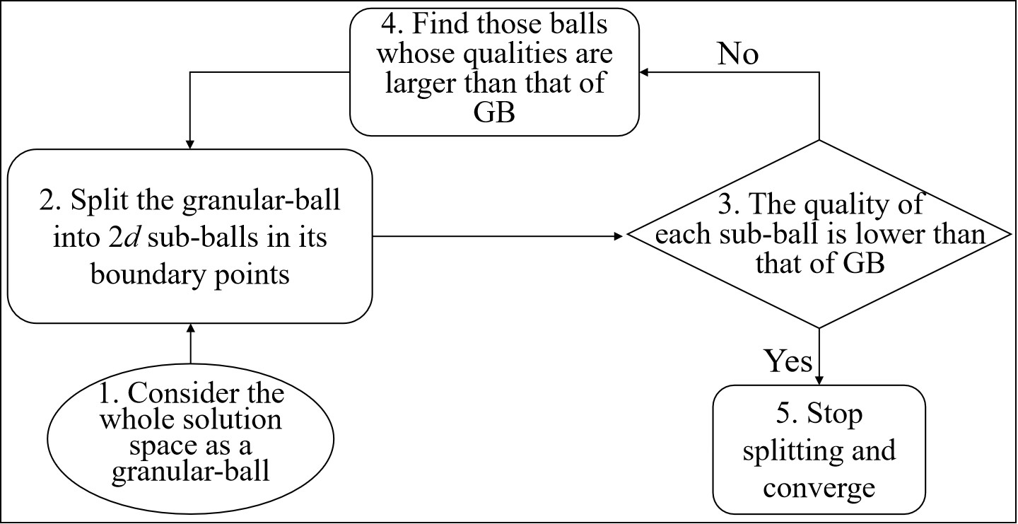
Figure 3: Flow chart of single round splitting of granular-ball.

Definition 2.

Given a granlar-ball $GB$ with its center as $c$ and radius as $r$ respectively. A granular-ball with its center as $sc$ and radius as $sr$ is called a sub-ball of $GB$ if:

$$sc=1/2*(c+bp),bp\in BP_{i}(GB),i=1,2,\dots,d$$ (4)

$$sr=1/2*r.$$ (5)

Take the function of one variable $y=x^{2}+2x-1,x\in[-3,3]$ as an example. First, as shown in Fig. 4(4(a)), at the beginning of the algorithm, a granular-ball $A$ is used to cover the whole solution space and its function value is calculated according to (4). Then, as shown in Fig. 4(4(b)), we split the initial granular-ball into four sub-balls, $A_{1}$, $A_{2}$, $A_{3}$, and $A_{4}$, in its four boundary points and calculate their function values respectively according to (4). As only $\hat{f}(A_{3})$ is not larger than $\hat{f}(A)$, $A_{3}$ is continuously split in Fig. 4(4(c)). As only $\hat{f}(A_{32})$ is not larger than $\hat{f}(A_{3})$, $A_{32}$ is continuously split in Fig. 4(4(d)). As $\hat{f}(A_{31})$, $\hat{f}(A_{33})$, and $\hat{f}(A_{34})$ are all larger than $\hat{f}(A_{3})$, GBO converges and all granular balls stop splitting. At this time, it can be observed that many small granular-balls are distributed at the minimum value of the function curve, and the objective function values of those balls can describe the minimum value of the function well.

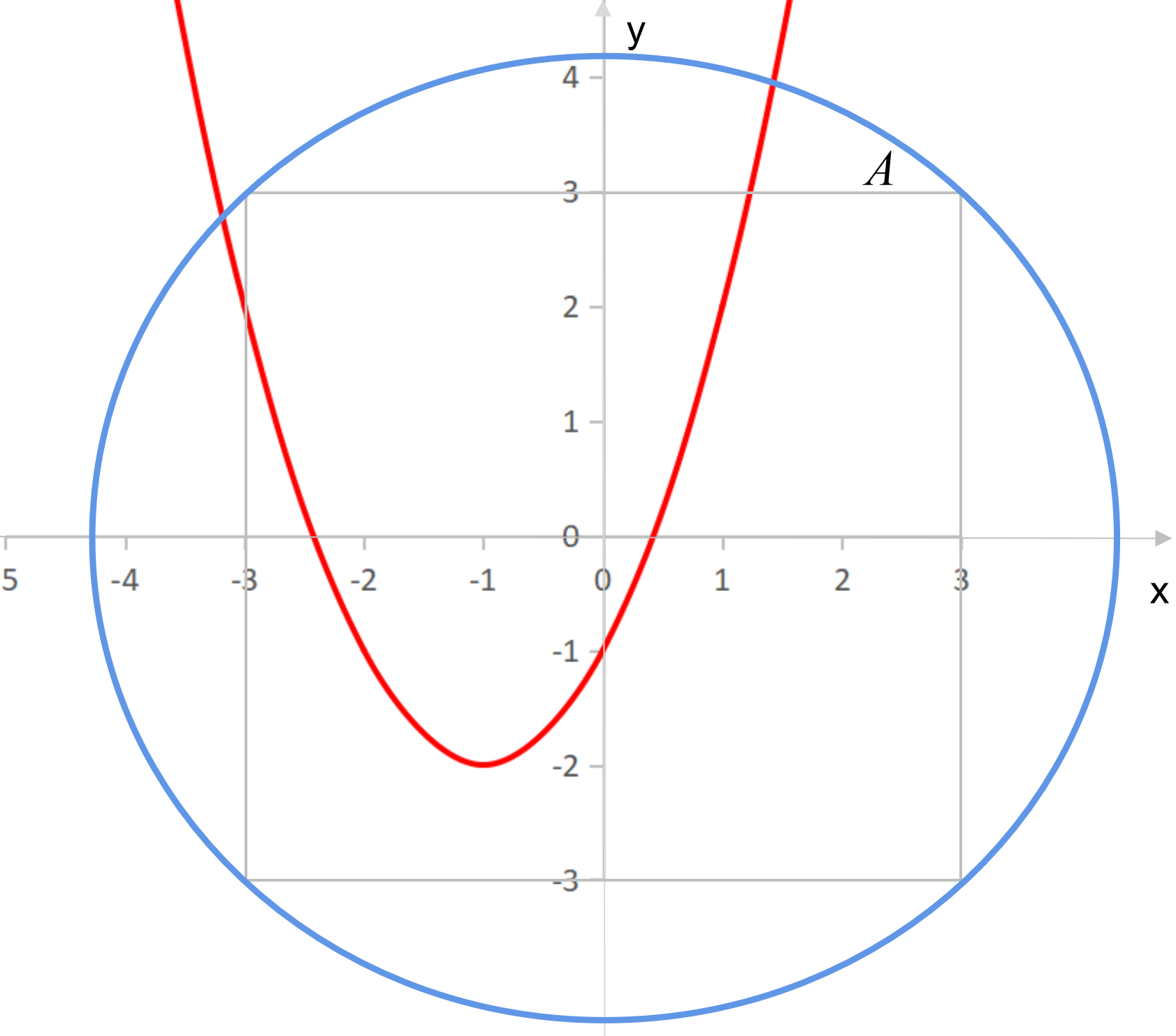
(a)

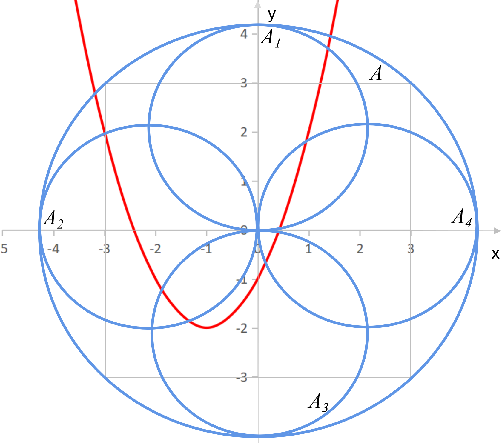
(b)

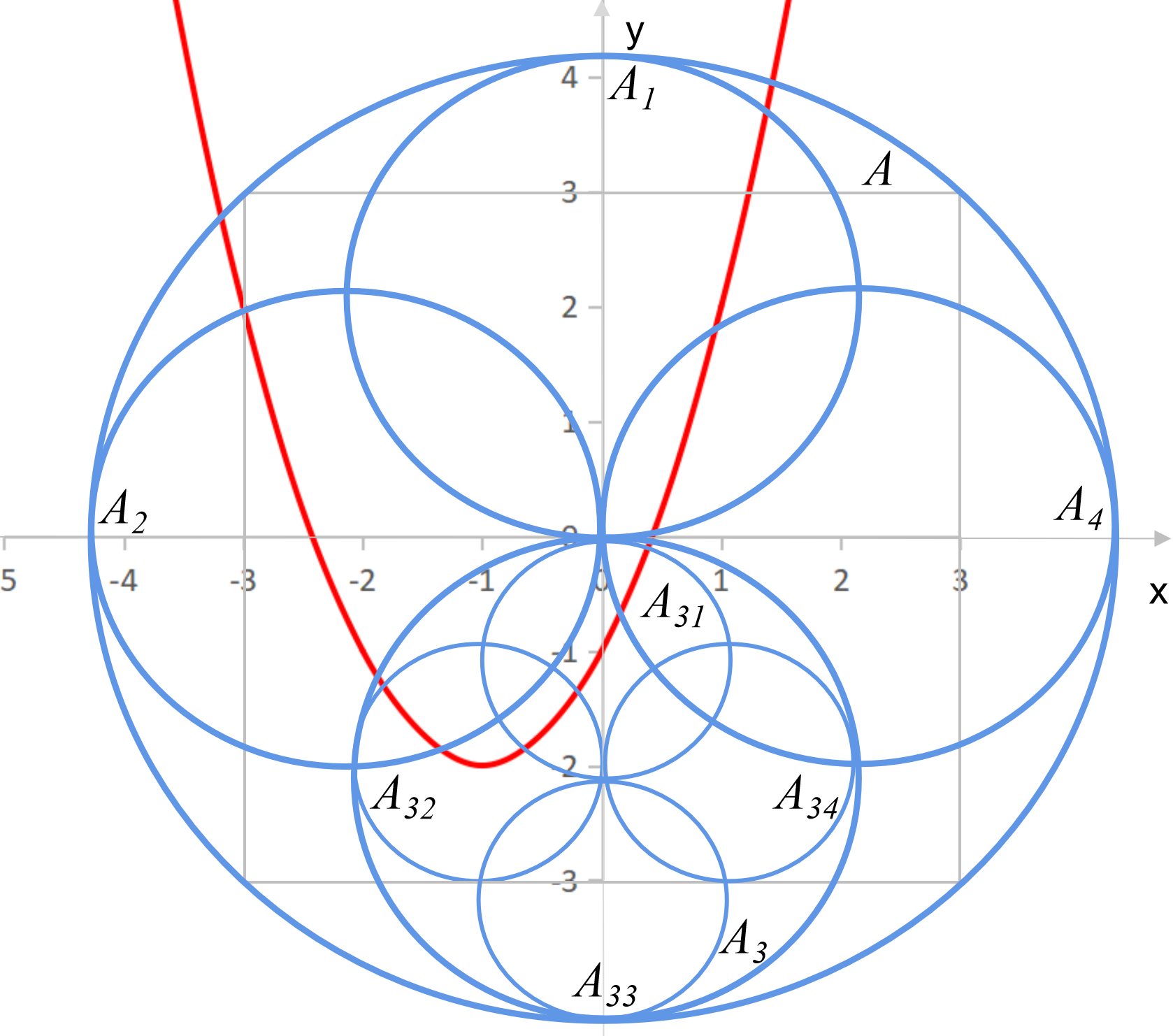
(c)

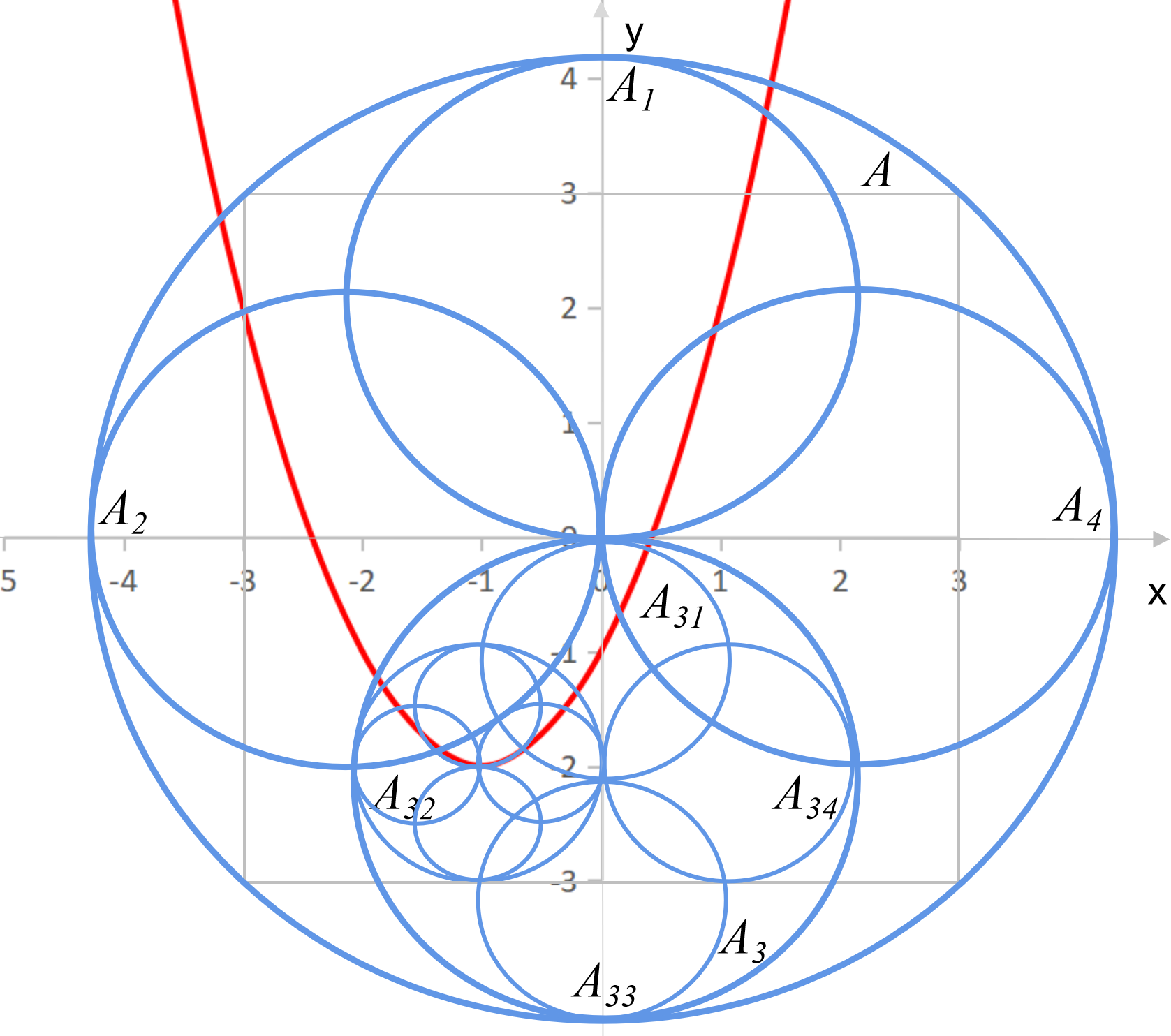
(d)

Figure 4: The diagram of granular-ball splitting. (4(a)) The initial granular-ball $A$. (4(b)) The result after $A$ is split. (4(c)) The result after $A_{3}$ is split. (4(d)) The result after $A_{32}$ is split.

GBO uses coarse-grained granular-balls instead of fine-grained sample points to search in the solution space, so the optimization process is more efficient than the existing methods. Besides, this coarse-to-fine splitting process covers the entire solution space, and can describe the overall multi-granularity distribution characteristics of data. As shown in Fig. 4(4(d)), the unimportant solution space is represented by a small number of coarse granular-balls, while the important solution space is represented by a large number of fine granular-balls. This multi-granularity description ability enables GBO to obtain better solutions than the existing methods. In addition, the whole process has no parameters. To sum up, the multi-granularity optimization process makes GBO efficient, accurate and adaptive. This will be further demonstrated in the experimental results. The GBO algorithm is provided in Algorithm 1.

Algorithm 1 Granular-ball Optimization Algorithm.

Input: The objective function $f(x_{1},x_{2},\dots,x_{d})$, $x_{i}\in[-a_{i},a_{i}]$;
Output: The minimum function value $f^{*}$ and the corresponding boundary point $bp^{*}$;

1:  $CurrentSet$ =Ø; $SubSet$ = Ø;

2:  Generate initial granular-ball $GB$ to cover the solution space, and $CurrentSet$ = $CurrentSet\cup GB$;

3:  $f^{*}$ = $\hat{f}(GB)$; ${bp}^{*}$= the boundary point that generates $\hat{f}(GB)$;

4:  for each granular-ball $GB_{i}$ in $CurrentSet$ do

5:     if $\hat{f}(GB_{i})<f^{*}$ then

6:        $f^{*}=\hat{f}(GB_{i})$; ${bp}^{*}$= the corresponding boundary point that generates $\hat{f}(GB)$;

7:     end if

8:     Split $GB_{i}$ and its sub-balls are denoted $GB_{i}Sub$;

9:     for each granular-ball $GB_{i}Sub_{j}$ in $GB_{i}Sub$ do

10:        if $\hat{f}(GB_{i}Sub_{j})<\hat{f}(GB_{i})$ then

11:           $SubSet$ = $SubSet\cup GB_{i}Sub_{j}$;

12:        end if

13:     end for

14:  end for

15:  if $SubSet$ $\neq$ Ø  then

16:     $CurrentSet=SubSet$; $SubSet=\text{\O}$; goto Step 4;

17:  else

18:     return $f^{*}$ and $bp^{*}$;

19:  end if

3.2.3 Improved Quality Evaluation of a Granular-ball

In Def. (2), the quality of a granular-ball is determined by its boundary points. However, in this way, the ability to describe the solution space inside the granular-ball may not be good enough. Therefore, more sub-balls are used to improve the quality of a granular-ball, the improved objective function value of a granular-ball is defined as follows.

Table 1: The twenty benchmark functions used in our experiment. Opt represents the theoretical global minimum of the function.

Function Name	Function Expression	Define Fields	Opt
Sphere Model	$f_{1}=\sum_{i=1}^{n}x_{i}^{2}$	$x_{i}\in[-100,100]$	0
Schwefel’s Problem 1.2	$f_{2}={\textstyle\sum_{i=1}^{n}}({\textstyle\sum_{j=1}^{i}}x_{j})^{2}$	$x_{i}\in[-100,100]$	0
Generalized Rosenbrock’s Function	$f_{3}={\textstyle\sum_{i=1}^{n-1}}[100(x_{i+1}-x_{i}^{2})^{2}+(x_{i}-1)^{2}]$	$x_{i}\in[-30,30]$	0
Quartic Function i.e. Noise	$f_{4}={\textstyle\sum_{i=1}^{n}}ix_{i}^{4}+random[0,1)$	$x_{i}\in[-1.28,1.28]$	0
Drop-Wave Function	$f_{5}=-\frac{1+\cos(12\sqrt{x_{1}^{2}+x_{2}^{2}})}{0.5(x_{1}^{2}+x_{2}^{2})+2}$	$x_{i}\in[-5.12,5.12]$	-1
Levy Function N. 13	$f_{6}=\sin^{2}(3\pi x_{1})+(x_{1}-1)^{2}\left[1+sin^{2}(3\pi x_{2})\right]+(x_{2}-1)^{2}[1+sin^{2}(2\pi x_{2})]$	$x_{1}\in[-10,10]$	0
Matyas Function	$f_{7}=0.26(x_{1}^{2}+x_{2}^{2})-0.48x_{1}x_{2}$	$x_{i}\in[-10,10]$	0
Three-Hump Camel Function	$f_{8}=2x_{1}^{2}-1.05x_{1}^{4}+\frac{x_{1}^{6}}{6}+x_{1}x_{2}+x_{2}^{2}$	$x_{i}\in[-10,10]$	0
Goldstein-Price Function	$f_{9}=[1+(x_{1}+x_{2}+1)^{2}(19-14x_{1}+3x_{1}^{2}-14x_{2}+6x_{1}x_{2}+3x_{2}^{2})]\times[30+(2x_{1}-3x_{2})^{2}(18-32x_{1}+12x_{1}^{2}+48x_{2}-36x_{1}x_{2}+27x_{2}^{2})]$	$x_{i}\in[-2,2]$	3
Schaffer Function N. 2	$f_{10}=0.5+\frac{\sin^{2}(x_{1}^{2}-x_{2}^{2})-0.5}{[1+0.001(x_{1}^{2}+x_{2}^{2})]^{2}}$	$x_{i}\in[-100,100]$	0
Generalized Rastrigin’s Function	$f_{11}=\sum_{i=1}^{30}\left[x_{i}^{2}-10\cos(2\pi x_{i})+10\right]$	$x_{i}\in[-5.12,5.12]$	0
Easom Function	$f_{12}=-\cos(x_{1})\cos(x_{2})\exp(-(x_{1}-\pi)^{2}-(x_{2}-\pi)^{2})$	$x_{i}\in[-100,100]$	-1
Sum of Different Powers Function	$f_{13}=\sum_{i=1}^{d}|x_{i}|^{i+1}$	$x_{i}\in[-1,1]$	0
Rastrigin Function	$f_{14}=10d+\sum_{i=1}^{d}[x_{i}^{2}-10\cos(2\pi x_{i})]$	$x_{i}\in[-5.12,5.12]$	0
Sum Squares Function	$f_{15}=\sum_{i=1}^{d}ix_{i}^{2}$	$x_{i}\in[-10,10]$	0
Generalized Griewank’s Function	$f_{16}=\frac{1}{4000}\sum_{i=1}^{30}x_{i}^{2}-\prod_{i=1}^{30}\cos(\frac{x_{i}}{\sqrt{i}})+1$	$x_{i}\in[-600,600]$	0
Rotated Hyper-Ellipsoid Function	$f_{17}=\sum_{i=1}^{d}\sum_{j=1}^{i}x_{j}^{2}$	$x_{i}\in[-65.536,65.536]$	0
Bohachevsky Function1	$f_{18}=x_{1}^{2}+2x_{2}^{2}-0.3\cos(3\pi x_{1})-0.4\cos(4\pi x_{2})+0.7$	$x_{i}\in[-100,100]$	0
Bohachevsky Function2	$f_{19}=x_{1}^{2}+2x_{2}^{2}-0.3\cos(3\pi x_{1})\cos(4\pi x_{2})+0.3$	$x_{i}\in[-100,100]$	0
Bohachevsky Function3	$f_{20}=x_{1}^{2}+2x_{2}^{2}-0.3\cos(3\pi x_{1}+4\pi x_{2})+0.3$	$x_{i}\in[-100,100]$	0

Definition 3.

Given a granular-ball $GB$ with its radius and center as $r$ and $c$. A granular-ball $GB^{{}^{\prime}}$ with its radius $r^{\prime}$ and $c^{\prime}$ is called the concentric sub-ball of $GB$ if $r^{\prime}<r$ and $c^{\prime}=c$. The concentric sub-balls of $GB$ contains $GB_{1}^{{}^{\prime}},GB_{2}^{{}^{\prime}},\dots,GB_{p}^{{}^{\prime}}$, where $p$ denotes the number of the sub-balls. The improved objective function value of $GB$, $\tilde{f}(GB)$, can be expressed as:

$$\tilde{f}(GB)=min(\hat{f}(GB_{i}^{{}^{\prime}})),i=1,2,\dots,p.$$ (6)

In Def. 3, for a granular-ball, its concentric sub-balls can be used to improve the description of the solution space in the granular-ball. For a granular-ball with center as $c$ and radius as $r$, its concentric sub-balls can be generated in the following ways: their centers are set to $c$, and their radii are generated by increasing from 0 to $r$ in a certain step. So, the core problem is how to set the step size. An intuitive way, as shown in Fig. 5(5(a)), is to set the step length to a fixed value, 1. However, this method will cause a lot of repeated calculations.

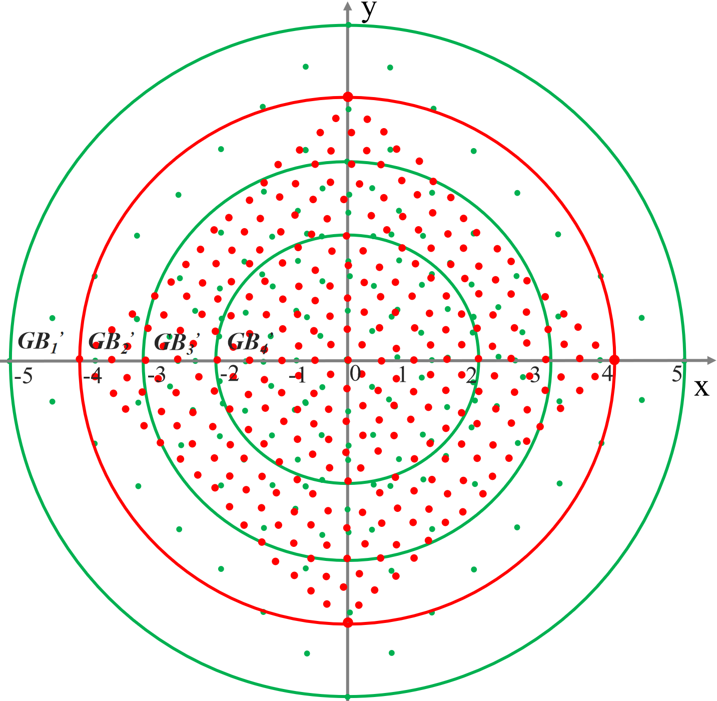
(a)

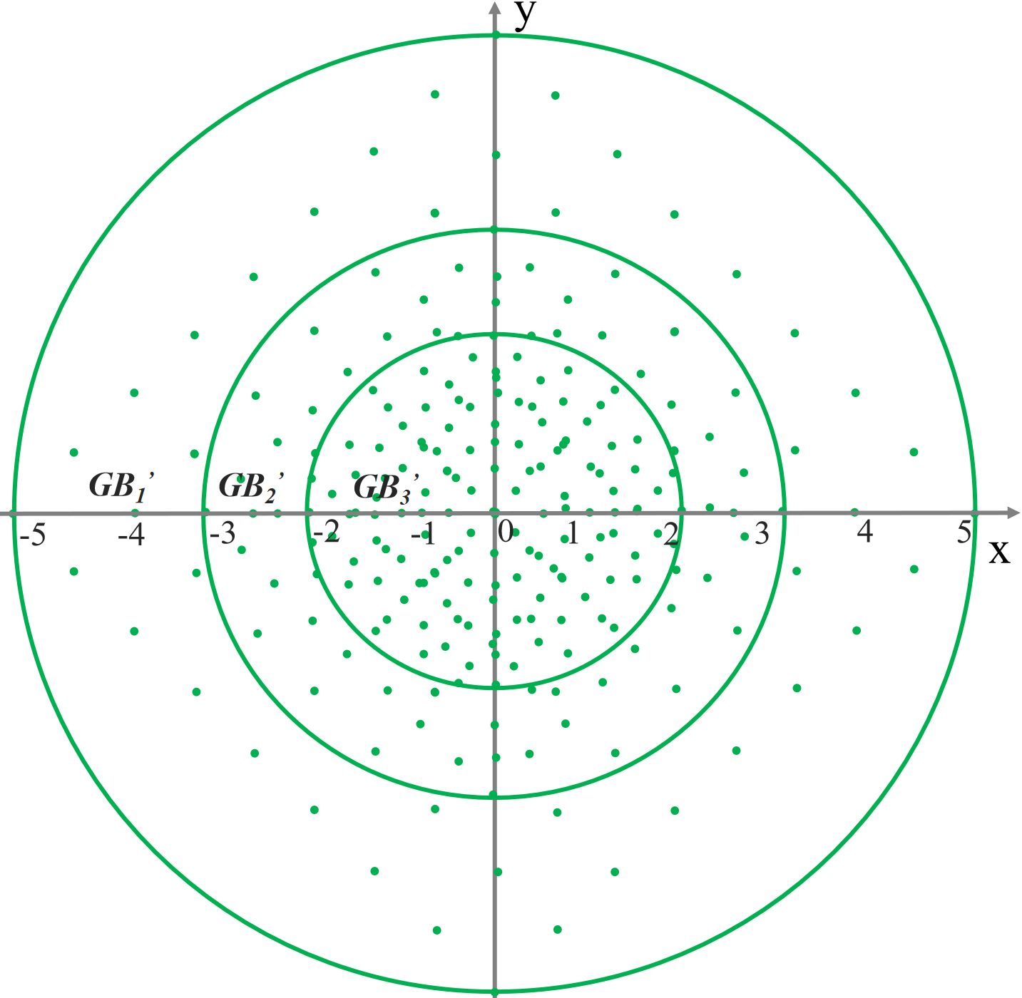
(b)

Figure 5: (5(a)) Schematic diagram of granular-ball splitting with fixed step size of $1$. (5(b)) Schematic diagram of granular-ball splitting based on primes. All points represent the boundary points of those sub-balls generated in multiple rounds splitting. All the computations of the objective function are in these points. Repeated calculation occur in those red points, and not in the green points.

In Fig. 5(5(a)), all calculated points in $r=2$ will be re-computed in $r=8$. Similarly, all points of $r=8$ will be repeated in $r=16$. In order to reduce double counting, we design a radius generation method based on prime numbers. In this method, for a granular-ball with radius as $R$, all primes of the range $(0,R)$ are respectively selected as the radii of its concentric granular-balls. As a prime is divisible only by $1$ and itself, there is no double computing; as shown in (5(b)), there are no red points.

4 Experiments

We evaluate the performance of the algorithms on twenty benchmark functions in comparison with those most widely used and the-state-of-the-art evolutionary algorithms, including PSOKennedy and Eberhart (1995),DEStorn (1996), AFSALi (2003), GAHolland (1992), SAVan Laarhoven and Aarts (1987) and FWALi and Tan (2017). Tab. 1 lists the basic information of the twenty benchmark functions including function name, function expression, define fields, and optimal value. A more detailed description for each function is provided in Appendix. $f_{1}$-$f_{4}$ are unimodal functions; $f_{4}$ is a noisy quartic function, and the variable $random$ in $f_{4}$ is uniformly distributed in $(0,1)$. $f_{5}$-$f_{20}$ are multi-modal functions. The hardware environment of the experiments is a PC with an Intel Core i7-6700HQ CPU @3.4GHz with 8G RAM; the experimental software is Python 3.9.All the results are conducted under the same conditions. To reduce the influence of the randomness of the bionic algorithm, we run ten times for each function and take the average, and the best results are displayed in bold.

4.1 Parameter Setting

The parameters of the comparison algorithms used in the experiments are shown in Tab. 2. All parameters of the comparison algorithms are set to default values. It should be noted that GBO does not contain any hyper-parameters. This leads to better performance of GBO in stability and adaptiveness in comparison with other algorithms.

Table 2: Parameter information. N denotes the number of parameters.

Algorithms	N	Parameter items
GBO	0	-
PSO	7	$size\_pop$, $max\_iter$, $w$, $c_{1}$, $c_{2}$, $lb$, $ub$
DE	6	$size\_pop$, $max\_iter$, $prob\_mut$, $F$, $lb$, $ub$
AFSA	7	$size\_pop$, $max\_iter$, $max\_try\_num$, $step$, $visual$, $q$, $delta$
GA	6	$size\_pop$, $max\_iter$, $prob\_mut$, $lb$, $ub$, $precision$
SA	7	$x_{0}$, $T\_max$, $T\_min$, $L$, $max\_stay\_counter$, $lb$, $ub$
FWA	7	$size\_pop$, $max\_iter$, $\lambda$, $\alpha$, $mu\_rate$, $c_{a}$, $c_{r}$

4.2 Effectiveness

In this section, the convergence error of the algorithms is compared, and the experimental results are shown in Tab. 3. The convergence error represents the difference between the optimization result and the theoretical optimal value. The smaller the error, the better the optimization result.

Table 3: Solution comparison between GBO and baselines on $f_{1}$–$f_{20}$. Min denotes the theoretical minimum.

Func	Min	GBO	PSO	DE	AFSA	GA	SA	FWA
$f_{1}$	0	0	7.98E-14	9.32E-20	1.85E-09	4.31E-04	8.83E-09	6.20E-31
$f_{2}$	0	0	1.23E-13	1.91E-09	8.22E-10	1.76E-01	8.54E-09	6.42E-31
$f_{3}$	0	0	4.09E+00	3.11E-02	5.60E-08	3.31E+00	0.00E+00	2.55E-30
$f_{4}$	0	2.30E-05	5.85E-04	4.08E-01	4.63E-03	6.12E-01	2.98E-04	3.70E-01
$f_{5}$	-1	-1	-9.94E-01	-9.99E-01	-9.41E-01	-9.04E-01	-9.94E-01	-1.00E+00
$f_{6}$	0	1.35E-31	9.86E-15	5.80E-22	3.16E-08	4.40E-02	1.35E-31	2.42E-31
$f_{7}$	0	0	3.27E-16	2.39E-09	1.18E-10	2.88E-02	2.26E-09	1.63E-33
$f_{8}$	0	0	5.22E-16	2.07E-16	2.86E-09	8.98E-02	2.00E-09	2.05E-32
$f_{9}$	3	3	3.00E+00	3.00E+00	3.00E+00	5.70E+00	3.00E+00	3.00E+00
$f_{10}$	0	0	2.22E-17	1.76E-06	1.31E-12	8.37E-02	1.04E-09	0.00E+00
$f_{11}$	0	0	2.13E-14	0.00E+00	4.73E-07	1.09E+00	7.15E-09	0.00E+00
$f_{12}$	-1	-6.78E-01	-1.00E+00	-1.00E+00	-2.15E-05	-2.00E-01	-7.09E-01	-3.18E-01
$f_{13}$	0	0	1.18E-18	4.75E-28	2.41E-11	5.90E-08	1.35E-10	1.27E-20
$f_{14}$	0	0	1.15E-13	0.00E+00	9.29E-07	1.09E+00	4.46E-09	0.00E+00
$f_{15}$	0	0	6.23E-16	5.64E-22	1.82E-09	5.22E-05	1.73E-09	2.27E-32
$f_{16}$	0	0	3.70E-03	5.76E-06	2.23E-09	2.34E-01	2.96E-03	4.14E-04
$f_{17}$	0	0	1.50E-14	1.02E-20	1.23E-09	1.51E-03	8.34E-09	2.83E-31
$f_{18}$	0	0	6.87E-13	0.00E+00	9.26E-08	1.88E-01	3.90E-08	0.00E+00
$f_{19}$	0	0	1.01E-12	1.59E-14	1.02E-09	1.79E-01	4.54E-08	0.00E+00
$f_{20}$	0	0	4.39E-12	6.24E-08	1.86E-09	2.00E-01	4.22E-08	0.00E+00

As shown in Tab. 3, the errors of GBO for $f_{1}$-$f_{3}$, $f_{5}$, $f_{7}$-$f_{11}$, and $f_{13}$-$f_{20}$ functions are all equal to $0$, which indicates the solutions of GBO are exactly consistent with the theoretical optimal values; in comparison, all other algorithms can not achieve this point. Besides, the solutions of GBO are much better than those of other comparison algorithms in almost all cases only except the case on $f_{12}$, no matter on which unimodal and multi-modal functions. Furthermore, even on $f_{12}$, the converge performance in the error has reached above average level, and better than those of AFSA, GA, SA, and FWA. In general, as shown in Tab. 3, the convergence accuracy of GBO algorithm is significantly higher than that of other algorithms. The reason is that, as GBO can simulate the multi-granularity distribution of data, the important part of the solution space is covered by a large amount of fine-grained granular-balls, which makes GBO have better search ability of the optimal solution than the existing intelligent optimization algorithms. In addition, another phenomenon is that the error of FWA is the closest to GBO and less than other algorithms. But at the same time, our subsequent experiments show that the time cost of FWA is also the highest due to the high frequency of optimization search; in contrast, while maintaining the minimum error, GBO is also significantly ahead of other algorithms in efficiency.

4.3 Efficiency

In this section, the convergence speed of the algorithms is compared, and their running time is shown in Tab. 4. As shown in Tab. 4, it can be observed that GBO is much faster than other algorithms on almost all the datasets except $f_{13}$ and $f_{16}$. Even on $f_{13}$ and $f_{16}$, the running time of GBO on the two functions (i.e.,$0.11s$ and $0.08s$ respectively) is also far below the average level, and only very close to the best case, ranking second. The reason is that, as GBO can simulate the multi-granularity distribution of data, the unimportant part of the solution space is covered by a small amount of coarse-grained granular-balls, which makes GBO avoid a large number of search calculations. So, it has a faster convergence speed than the existing intelligent optimization algorithms.

Table 4: The comparison of running time (s).

Func	GBO	PSO	DE	AFSA	GA	SA	FWA
$f_{1}$	0.00	0.02	0.07	7.96	0.16	0.52	73.64
$f_{2}$	0.01	0.02	0.06	7.71	0.15	0.57	77.95
$f_{3}$	0.00	0.02	0.08	7.32	0.16	0.57	86.98
$f_{4}$	0.00	0.02	0.07	2.75	0.14	0.55	89.92
$f_{5}$	0.00	0.04	0.15	3.14	0.19	0.62	132.86
$f_{6}$	0.03	0.05	0.16	12.43	0.20	0.69	161.20
$f_{7}$	0.00	0.02	0.07	8.30	0.15	0.55	83.18
$f_{8}$	0.00	0.03	0.09	9.29	0.15	0.59	95.65
$f_{9}$	0.04	0.04	0.14	10.17	0.19	0.66	150.97
$f_{10}$	0.01	0.03	0.12	11.74	0.17	0.57	118.19
$f_{11}$	0.00	0.04	0.13	10.71	0.18	0.58	127.70
$f_{12}$	0.03	0.04	0.14	2.70	0.18	0.55	137.22
$f_{13}$	0.11	0.03	0.11	10.41	0.17	0.51	108.52
$f_{14}$	0.00	0.03	0.13	10.82	0.19	0.56	126.30
$f_{15}$	0.00	0.02	0.07	8.02	0.15	0.49	79.80
$f_{16}$	0.08	0.05	0.17	14.95	0.21	0.65	150.48
$f_{17}$	0.00	0.02	0.07	8.39	0.15	0.50	81.94
$f_{18}$	0.01	0.04	0.13	10.22	0.20	0.58	125.41
$f_{19}$	0.01	0.03	0.12	9.65	0.21	0.56	122.22
$f_{20}$	0.04	0.04	0.11	9.63	0.20	0.55	105.82

4.4 Stability and Adaptiveness

In this section, two unimodal functions $f_{3}$ and $f_{4}$, and two complex multi-modal functions $f_{5}$ and $f_{11}$ are selected for verify the stability of the comparison algorithms. The function diagram of $f_{3}$, $f_{4}$, $f_{5}$, and $f_{11}$ are shown in Fig. 6. Each algorithm is executed for 10 rounds in four functions and count its optimization error in Fig. 7, and the average error of the ten rounds in Fig. 8. As the running time of different algorithms is quite different, in order to display conveniently in the same figure, we have taken the logarithm of the running time with base 10 and displayed it in Fig. 7. Besides, as some convergence error values of GBO are equal to $0$, we add a minimum value $1E-31$ to all errors in the process of taking logarithm. The raw data of running time is provided in Tab. 1 in the appendix.

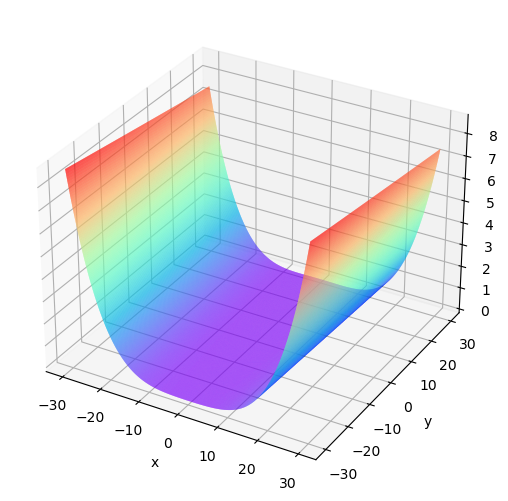
(a)

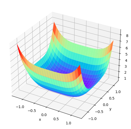
(b)

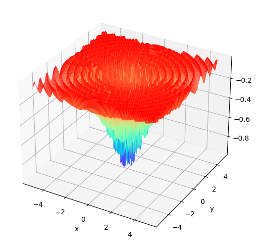
(c)

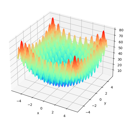
(d)

Figure 6: Function diagrams of $f_{3}$, $f_{4}$, $f_{5}$, and $f_{11}$, corresponding to (6(a)), (6(b)), (6(c)) and (6(d)) respectively.

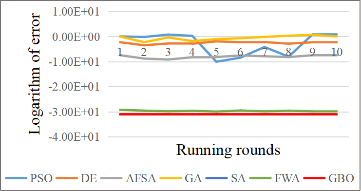
(a)

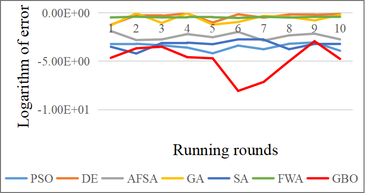
(b)

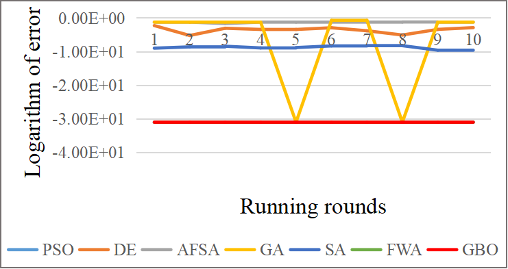
(c)

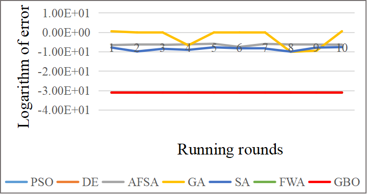
(d)

Figure 7: The error of GBO and baselines running ten times on function $f_{3}$, $f_{4}$, $f_{5}$, and $f_{11}$, corresponding to (7(a)), (7(b)), (7(c)) and (7(d)).

As shown in Fig. 7(7(a)), (7(c)), and (7(d)), the error of GBO is much smaller and stable than other algorithms. The instability of GBO in Fig. 7(7(b)) comes from the using of a random function in $f_{4}$. In general, GBO has the best performance in stability. The experimental results about the average error in Fig. 8 also support this conclusion. The reason is that GBO does not contain any hyper-parameters and random factors. In addition, not containing any hyper-parameters also makes GBO completely adaptive, which is an important characteristics that other intelligence optimization algorithms does not have.

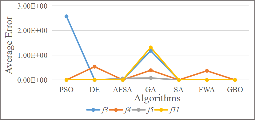
Figure 8: The average error of running ten rounds of the comparison algorithms for $f_{3}$, $f_{4}$, $f_{5}$, and $f_{11}$ functions.

5 Conclusions and Future Work

This paper presents a multi-granularity optimization algorithm GBO which can simulate the multi-granularity distribution of data. Different from the existing intelligence optimization algorithms, its optimization process is based on granular-balls with different sizes, rather than sampling points. This leads to better convergence performance both in convergence speed and convergence accuracy than the existing algorithms. GBO contains no hyper-parameters, so it is completely adaptive and more stable than other algorithms. The experimental results in 20 benchmark functions show that GBO is significantly better than the existing algorithms in terms of both convergence speed and accuracy.

At present, GBO is just a new and simple basic method. In future work, we will further develop it and improve its performance to solve high-dimensional and multi-modal function optimization. In addition, a better ball splitting strategy may bring higher convergence accuracy, which deserves further study.

6 Appendix

• Sphere Model

  $$\begin{split}f_{1}(x)=\sum_{i=1}^{n}x_{i}^{2},\ \ x_{i}\in[-100,100]\ \ \ \ \ \ \\ min(f_{1})=f_{1}(0,0)=0.\ \ \ \ \ \ \ \ \ \ \ \ \end{split}$$

• Schwefel’s Problem 2.22

  $$\begin{split}f_{2}(x)={\textstyle\sum_{i=1}^{n}}({\textstyle\sum_{j=1}^{i}}x_{j})^{2},\ \ x_{i}\in[-100,100]\\ min(f_{2})=f_{2}(0,0)=0.\ \ \ \ \ \ \ \ \ \ \ \ \ \ \ \ \ \ \end{split}$$

• Generalized Rosenbrock’s Function

  $$\begin{split}f_{3}(x)={\textstyle\sum_{i=1}^{n-1}}[100(x_{i+1}-x_{i}^{2})^{2}+(x_{i}-1)^{2}],\\ x_{i}\in[-30,30],min(f_{3})=f_{3}(1,1)=0.\ \ \ \ \ \ \end{split}$$

• Quartic Function i.e. Noise

  $$\begin{split}f_{4}(x)={\textstyle\sum_{i=1}^{n}}ix_{i}^{4}+random[0,1),\ \ \ \ \ \ \ \ \ \\ x_{i}\in[-1.28,1.28],min(f_{4})=f_{4}(0,0)=0.\end{split}$$

• Cross-in-Tray Function

  $$\begin{split}f_{5}(x)=-\frac{1+\cos(12\sqrt{x_{1}^{2}+x_{2}^{2}})}{0.5(x_{1}^{2}+x_{2}^{2})+2}\ \ \ \ \ \ \ \ \ \ \ \ \ \\ x_{i}\in[-5.12,5.12],\ \ min(f_{5})=f_{5}(0,0)=-1.\end{split}$$

• Levy Function N. 13

  $$\begin{split}f_{6}(x)=\sin^{2}(3\pi x_{1})+(x_{1}-1)^{2}\left[1+sin^{2}(3\pi x_{2})\right]\\ +(x_{2}-1)^{2}[1+sin^{2}(2\pi x_{2})]\ \ \ \ \ \ \ \ \ \ \ \ \ \ \ \ \ \ \ \ \\ x_{i}\in[-10,10],\ \ min(f_{6})=f_{6}(1,1)=0.\ \ \ \ \ \ \ \ \ \end{split}$$

• Matyas Function

  $$\begin{split}f_{7}(x)=0.26(x_{1}^{2}+x_{2}^{2})-0.48x_{1}x_{2}\ \ \ \ \ \ \\ x_{i}\in[-10,10],\ \ min(f_{7})=f_{7}(0,0)=0.\end{split}$$

• Three-Hump Camel Function

  $$\begin{split}f_{8}(x)=2x_{1}^{2}-1.05x_{1}^{4}+\frac{x_{1}^{6}}{6}+x_{1}x_{2}+x_{2}^{2}\ \ \ \ \ \\ x_{i}\in[-10,10],\ \ min(f_{8})=f_{8}(0,0)=0.\ \ \ \ \end{split}$$

• Goldstein-Price Function

  $$\begin{split}f_{9}(x)=[1+(x_{1}+x_{2}+1)^{2}(19-14x_{1}+3x_{1}^{2}\\ -14x_{2}+6x_{1}x_{2}+3x_{2}^{2})]\times[30+(2x_{1}-3x_{2})^{2}\\ (18-32x_{1}+12x_{1}^{2}+48x_{2}-36x_{1}x_{2}+27x_{2}^{2})]\\ x_{i}\in[-2,2],\ \ min(f_{9})=f_{9}(0,-1)=3.\ \ \ \ \ \end{split}$$

• Styblinski-Tang Function

  $$\begin{split}f_{10}(x)=0.5+\frac{\sin^{2}(x_{1}^{2}-x_{2}^{2})-0.5}{[1+0.001(x_{1}^{2}+x_{2}^{2})]^{2}}\ \ \ \ \ \ \\ x_{i}\in[-100,100],\ \ min(f_{10})=f_{10}(0,0)=0.\end{split}$$

• Generalized Rastrigin’s Function

  $$\begin{split}f_{18}(x)=\sum_{i=1}^{30}\left[x_{i}^{2}-10\cos(2\pi x_{i})+10\right]\ \ \ \ \ \ \ \ \\ x_{i}\in[-5.12,5.12],\ \ min(f_{18})=f_{18}(0,0)=0.\end{split}$$

• Easom Function

  $$\begin{split}f_{12}(x)=-\cos(x_{1})\cos(x_{2})\exp(-(x_{1}-\pi)^{2}-(x_{2}-\pi)^{2})\\ x_{i}\in[-100,100],\ \ min(f_{12})=f_{12}(\pi,\pi)=-1.\ \ \ \ \ \ \ \ \ \ \end{split}$$

• Sum of Different Powers Function

  $$\begin{split}f_{13}(x)=\sum_{i=1}^{d}|x_{i}|^{i+1},x_{i}\in[-1,1]\ \ \ \ \ \ \\ min(f_{13})=f_{13}(0,0)=0.\ \ \ \ \ \ \ \ \ \ \ \end{split}$$

• Rastrigin Function

  $$\begin{split}f_{14}(x)=10d+\sum_{i=1}^{d}[x_{i}^{2}-10\cos(2\pi x_{i})]\ \ \ \ \ \ \ \ \\ x_{i}\in[-5.12,5.12],\ \ \ \ \ \ \ \ \ \ \ \ \ \ \ \ \ \ \ \ \ \ \ \ \ \ \\ min(f_{14})=f_{14}(0.00034,0.00014)=0.\ \ \ \ \ \ \ \end{split}$$

• Sum Squares Function

  $$\begin{split}f_{15}(x)=\sum_{i=1}^{d}ix_{i}^{2},\ \ x_{i}\in[-10,10]\ \ \ \ \ \\ min(f_{15})=f_{15}(0,0)=0.\ \ \ \ \ \ \ \ \ \ \end{split}$$

• Generalized Griewank’s Function

  $$\begin{split}f_{16}(x)=\frac{1}{4000}\sum_{i=1}^{30}x_{i}^{2}-\prod_{i=1}^{30}\cos(\frac{x_{i}}{\sqrt{i}})+1\ \ \ \ \ \ \\ x_{i}\in[-600,600],\ \ min(f_{16})=f_{16}(0,0)=0.\end{split}$$

• Rotated Hyper-Ellipsoid Function

  $$\begin{split}f_{17}(x)=\sum_{i=1}^{d}\sum_{j=1}^{i}x_{j}^{2},\ \ x_{i}\in[-65.536,65.536]\\ min(f_{17})=f_{17}(0,0)=0.\ \ \ \ \ \ \ \ \ \ \ \ \end{split}$$

• Bohachevsky Function1

  $$\begin{split}f_{11}(x)=x_{1}^{2}+2x_{2}^{2}-0.3\cos(3\pi x_{1})-0.4\cos(4\pi x_{2})+0.7\\ x_{i}\in[-100,100],\ \ min(f_{11})=f_{11}(0,0)=0.\ \ \ \ \ \ \ \ \ \ \end{split}$$

• Bohachevsky Function2

  $$\begin{split}f_{19}(x)=x_{1}^{2}+2x_{2}^{2}-0.3\cos(3\pi x_{1})\cos(4\pi x_{2})+0.3\\ x_{i}\in[-100,100],\ \ min(f_{19})=f_{19}(0,0)=0.\ \ \ \ \ \ \end{split}$$

• Bohachevsky Function3

  $$\begin{split}f_{20}(x)=x_{1}^{2}+2x_{2}^{2}-0.3\cos(3\pi x_{1}+4\pi x_{2})+0.3\\ x_{i}\in[-100,100],\ \ min(f_{20})=f_{20}(0,0)=0.\ \ \ \end{split}$$

References

- Chen [1982] Lin Chen. Topological structure in visual perception. Science, 218(4573):699–700, 1982.
- Cheng et al. [2017] Ran Cheng, Miqing Li, Ke Li, and Xin Yao. Evolutionary multiobjective optimization-based multimodal optimization: Fitness landscape approximation and peak detection. IEEE Transactions on Evolutionary Computation, 22(5):692–706, 2017.
- Holland [1992] John H Holland. Genetic algorithms. Scientific american, 267(1):66–73, 1992.
- Huband et al. [2006] Simon Huband, Philip Hingston, Luigi Barone, and Lyndon While. A review of multiobjective test problems and a scalable test problem toolkit. IEEE Transactions on Evolutionary Computation, 10(5):477–506, 2006.
- Hussien et al. [2020] Abdelazim G Hussien, Mohamed Amin, and Mohamed Abd El Aziz. A comprehensive review of moth-flame optimisation: variants, hybrids, and applications. Journal of Experimental & Theoretical Artificial Intelligence, 32(4):705–725, 2020.
- Kennedy and Eberhart [1995] James Kennedy and Russell Eberhart. Particle swarm optimization. In Proceedings of ICNN’95-international conference on neural networks, volume 4, pages 1942–1948. IEEE, 1995.
- Li and Tan [2017] Junzhi Li and Ying Tan. Loser-out tournament-based fireworks algorithm for multimodal function optimization. IEEE Transactions on Evolutionary Computation, 22(5):679–691, 2017.
- Li et al. [2020] Hui Li, Peng Zou, Zhiguo Huang, Chenbo Zeng, and Xiao Liu. Multimodal optimization using whale optimization algorithm enhanced with local search and niching technique. Mathematical Biosciences and Engineering, 17(1):1–27, 2020.
- Li [2003] XL Li. A new intelligent optimization-artificial fish swarm algorithm. Doctor thesis, Zhejiang University of Zhejiang, China, 27, 2003.
- Qu et al. [2012] Bo-Yang Qu, Jing J Liang, and Ponnuthurai N Suganthan. Niching particle swarm optimization with local search for multi-modal optimization. Information Sciences, 197:131–143, 2012.
- Rashedi et al. [2018] Esmat Rashedi, Elaheh Rashedi, and Hossein Nezamabadi-Pour. A comprehensive survey on gravitational search algorithm. Swarm and evolutionary computation, 41:141–158, 2018.
- Shuyin et al. [2022] Xia Shuyin, Wang Cheng, Wang GuoYing, Gao XinBo, Elisabeth Giem, and Yu JianHang. Gbrs: An unified model of pawlak rough set and neighborhood rough set. arXiv preprint arXiv:2201.03349, 2022.
- Song et al. [2019] Zhaoyun Song, Bo Liu, and Hao Cheng. Adaptive particle swarm optimization with population diversity control and its application in tandem blade optimization. Proceedings of the Institution of Mechanical Engineers, Part C: Journal of Mechanical Engineering Science, 233(6):1859–1875, 2019.
- Storn [1996] Rainer Storn. Differential evolution design of an iir-filter. In Proceedings of IEEE international conference on evolutionary computation, pages 268–273. IEEE, 1996.
- Van den Bergh and Engelbrecht [2004] Frans Van den Bergh and Andries P Engelbrecht. A cooperative approach to particle swarm optimization. IEEE transactions on evolutionary computation, 8(3):225–239, 2004.
- Van Laarhoven and Aarts [1987] Peter JM Van Laarhoven and Emile HL Aarts. Simulated annealing. In Simulated annealing: Theory and applications, pages 7–15. Springer, 1987.
- Wang et al. [2013] Hui Wang, Wenjun Wang, and Zhijian Wu. Particle swarm optimization with adaptive mutation for multimodal optimization. Applied Mathematics and Computation, 221:296–305, 2013.
- Wang [2017] Guoyin Wang. Dgcc: data-driven granular cognitive computing. Granular Computing, 2(4):343–355, 2017.
- Weile and Michielssen [1997] Daniel S Weile and Eric Michielssen. Genetic algorithm optimization applied to electromagnetics: A review. IEEE Transactions on Antennas and Propagation, 45(3):343–353, 1997.
- Xia et al. [2019] Shuyin Xia, Yunsheng Liu, Xin Ding, Guoyin Wang, Hong Yu, and Yuoguo Luo. Granular ball computing classifiers for efficient, scalable and robust learning. Information Sciences, 483:136–152, 2019.
- Xia et al. [2020] Shuyin Xia, Daowan Peng, Deyu Meng, Changqing Zhang, Guoyin Wang, Elisabeth Giem, Wei Wei, and Zizhong Chen. A fast adaptive k-means with no bounds. IEEE Transactions on Pattern Analysis and Machine Intelligence, 2020.
- Xia et al. [2021] Shuyin Xia, Shaoyuan Zheng, Guoyin Wang, Xinbo Gao, and Binggui Wang. Granular ball sampling for noisy label classification or imbalanced classification. IEEE Transactions on Neural Networks and Learning Systems, 2021.
- Xia et al. [2022a] Shuyin Xia, Xiaochuan Dai, Guoyin Wang, Xinbo Gao, and Elisabeth Giem. An efficient and adaptive granular-ball generation method in classification problem. arXiv preprint arXiv:2201.04343, 2022.
- Xia et al. [2022b] Shuyin Xia, Xiaoyu Lian, and Yabin Shao. Fuzzy granular-ball computing framework and its implementation in svm. arXiv preprint arXiv:2210.11675, 2022.
- Xia et al. [2022c] Shuyin Xia, Guoyin Wang, Xinbo Gao, and Xiaoli Peng. Gbsvm: Granular-ball support vector machine. arXiv preprint arXiv:2210.03120, 2022.
- Yang et al. [2016] Qiang Yang, Wei-Neng Chen, Zhengtao Yu, Tianlong Gu, Yun Li, Huaxiang Zhang, and Jun Zhang. Adaptive multimodal continuous ant colony optimization. IEEE Transactions on Evolutionary Computation, 21(2):191–205, 2016.
- Zhang et al. [2013] YingChao Zhang, Xiong Xiong, and QiDong Zhang. An improved self-adaptive pso algorithm with detection function for multimodal function optimization problems. Mathematical Problems in Engineering, 2013, 2013.
- Zhang et al. [2020] Xu-Tao Zhang, Biao Xu, Wei Zhang, Jun Zhang, and Xin-fang Ji. Dynamic neighborhood-based particle swarm optimization for multimodal problems. Mathematical Problems in Engineering, 2020, 2020.
- Zhou et al. [2016] ZD Zhou, YQ Xie, DT Pham, Silah Kamsani, and Marco Castellani. Bees algorithm for multimodal function optimisation. Proceedings of the Institution of Mechanical Engineers, Part C: Journal of Mechanical Engineering Science, 230(5):867–884, 2016.