LON³LO

IFIC/23-11

FTUV-23-0321.0606

Drell–Yan lepton-pair production:
$\bf q_{T}$ resummation at approximate N⁴LL+N⁴LO accuracy

Stefano Camarda^(a), Leandro Cieri^(b) and Giancarlo Ferrera^(c)

^(a) CERN, CH-1211 Geneva, Switzerland

^(b) Instituto de Física Corpuscular, Universitat de València - Consejo Superior de Investigaciones Científicas, Parc Científic, E-46980 Paterna, Valencia, Spain

^(c) Dipartimento di Fisica, Università di Milano and

INFN, Sezione di Milano, I-20133 Milan, Italy

Abstract

We consider Drell–Yan lepton pairs produced in hadronic collisions. We present high-accuracy QCD predictions for the transverse-momentum ($q_{T}$) distribution and fiducial cross sections in the small $q_{T}$ region. We resum to all perturbative orders the logarithmically enhanced contributions up to the next-to-next-to-next-to-next-to-leading logarithmic (N⁴LL) accuracy and we include the hard-virtual coefficient at the next-to-next-to-next-to-leading order (N³LO) (i.e. $\mathcal{O}(\alpha_{S}^{3})$) with an approximation of the N⁴LO coefficients. The massive axial-vector and vector contributions up to three loops have also been consistently included. The resummed partonic cross section is convoluted with approximate N³LO parton distribution functions. We show numerical results at LHC energies of resummed $q_{T}$ distributions for $Z/\gamma^{*},W^{\pm}$ production and decay, including the $W^{\pm}$ and $Z/\gamma^{*}$ ratio, estimating the corresponding uncertainties from missing higher orders corrections and from incomplete or missing perturbative information coefficients at N⁴LL and N⁴LO. Our resummed calculation has been encoded in the public numerical program DYTurbo.

March 2023

The production of high invariant mass ($M$) lepton pairs in hadronic collision, through the Drell–Yan (DY) mechanism [1, 2], is extremely important for physics studies at hadron colliders and attracted a great deal of attention from the experimental and theory communities. Since the early days of QCD remarkable efforts have been devoted to detailed calculations of the dominant QCD higher-order radiative corrections of fiducial cross sections and kinematical distributions.

A sufficiently inclusive cross section can be perturbatively computable as an expansion in the QCD coupling $\alpha_{S}=\alpha_{S}(\mu_{R}^{2})$ where the normalization scale $\mu_{R}$ is of the order of the invariant mass $M$. However the bulk of experimental data lies in the small transverse momentum ($q_{T}$) region $q_{T}\ll M$ where the fixed-order expansion is spoiled by the presence of enhanced logarithmic corrections, $\alpha_{S}^{n}\ln^{m}(M^{2}/q_{T}^{2})$ of soft and collinear origin. In order to obtain reliable predictions, these logarithmic terms have to be systematically resummed to all orders in perturbation theory [3, 4, 5] (resummed calculation and studies applying different formalism and various levels of theoretical accuracy have been performed in Refs. [6, 7, 8, 9, 10, 11, 12, 13, 14, 15, 16, 17, 18, 19, 20, 21, 22, 23, 24, 25, 26, 27, 28, 29, 30, 31, 32].

In this paper we consider the Drell–Yan lepton pair production in the small $q_{T}$ region and we apply the QCD transverse-momentum resummation formalism developed in Refs. [6, 8, 17]. We resum all the logarithmically enhanced contributions up to the next-to-next-to-next-to-next-to-leading logarithmic (N⁴LL) accuracy and we include the hard-virtual coefficient at the next-to-next-to-next-to-leading order (N³LO) (i.e. $\mathcal{O}(\alpha_{S}^{3})$) with an estimate of the N⁴LO effects.

In the $Z$ boson case, because of the axial coupling, Feynman diagrams with quark loops contribute to the cross-section at $\mathcal{O}(\alpha_{S}^{2})$ and $\mathcal{O}(\alpha_{S}^{3})$. These contributions, also known as singlet contributions, cancel out for each isospin multiplet when massless quarks are considered. The effect of a finite top-quark mass in the third generation has been considered at $\mathcal{O}(\alpha_{S}^{2})$ in Refs. [33, 34] and has been found extremely small compared to the NNLO corrections. However these effects are not completely negligible when compared to the N³LO corrections [30]. We have considered the effect of a finite top-quark mass including in our calculation the singlet contributions up to $\mathcal{O}(\alpha_{S}^{3})$ by using the calculation of the quark axial form factor in QCD up to three loops [35]. We consistently included also the quark-loop mediated three-loop singlet corrections which contribute, via vector coupling, both to $Z$ and $\gamma^{*}$ production at $\mathcal{O}(\alpha_{S}^{3})$  [36, 37]

At large value of $q_{T}$ ($q_{T}\sim M$) fixed-order perturbative expansion is fully justified. In this region, the QCD radiative corrections are known up to $\mathcal{O}(\alpha_{S}^{3})$ numerically through the fully exclusive NNLO calculation of vector boson production in association with jets [38, 39, 40, 41, 42, 43, 44, 45, 31]. In particular the calculation of $Z+jet$ production at NNLO has been encoded in the public code MCFM [31]. Resummed and fixed-order calculation have to be consistently (i.e. avoiding double counting) matched at intermediate values of $q_{T}$ in order to obtain theoretical predictions with uniform accuracy over the entire range of $q_{T}$.

Our resummed calculation for $Z/\gamma^{*}$ and $W^{\pm}$ production and decay up to approximated N⁴LL+N⁴LO accuracy, together with the asymptotic expansion up to $\mathcal{O}(\alpha_{S}^{3})$, has been implemented in the public numerical program DYTurbo [46, 47] which provides fast and numerically precise predictions including the full kinematical dependence of the decaying lepton pair with the corresponding spin correlations and the finite value of the $Z$ boson width.

In this paper we are focusing on the impact of the N⁴LL resummed logarithmic terms. We thus consider only the the small $q_{T}$ region and we not include the matching with fixed-order predictions which can be implemented starting from the results of Refs. [38, 39, 40, 41, 42, 43, 44, 45, 31] and subtracting the asymptotic expansion of the resummed calculation at the same perturbative order as encoded in DYTurbo. Resummed results at N³LL +N³LO matched with the NNLO calculation at large $q_{T}$ have been presented in Refs. [48]. Here we extend the results of Ref. [48] by extending the resummation accuracy at approximated N⁴LL+N⁴LO and by presenting results for $W^{\pm}$ boson production and decay. A brief review of the resummation formalism of Refs. [6, 8, 17] is given in Appendix A together with a collection of the numerical coefficients needed at N⁴LL+N⁴LO accuracy.

In the following we consider $Z/\gamma^{*},W^{\pm}$ production and leptonic decay at the Large Hadron Collider (LHC). We present resummed predictions up to N⁴LL accuracy including the hard-virtual coefficient up to N³LO together with an approximation of the N⁴LO ones. The hadronic cross section is obtained by convoluting the partonic cross section in Eq. (7) with the parton densities functions (PDFs) from MSHT20aN3LO set [49] at the approximate N³LO with $\alpha_{S}(m_{Z}^{2})=0.118$ where we have evaluated $\alpha_{S}(\mu_{R}^{2})$ at $(n\!+\!1)$-loop order at NⁿLL accuracy. We use the so called $G_{\mu}$ scheme for EW couplings with input parameters $G_{F}=1.1663787\times 10^{-5}$ GeV^-2, $m_{Z}=91.1876$ GeV, $\Gamma_{Z}=2.4952$ GeV, $m_{W}=80.379$ GeV, $\Gamma_{W}=2.091$ GeV. In the case of $W$ production, we use the following CKM matrix elements: $V_{ud}=0.97427$, $V_{us}=0.2253$, $V_{ub}=0.00351$, $V_{cd}=0.2252$, $V_{cs}=0.97344$, $V_{cb}=0.0412$. We work with $N_{f}=5$ massless quarks and we use $m_{top}=173$ GeV for the top-loop mediated singlet contributions. Our calculation implements the leptonic decays $Z/\gamma^{*}\to l^{+}l^{-}$, $W\pm\to l\nu$ and we include the effects of the $Z/\gamma^{*}$ interference and of the finite widths of the $W$ and $Z$ boson with the corresponding spin correlations and the full dependence on the kinematical variables of final state leptons. This allows us to take into account the typical kinematical cuts on final state leptons that are considered in the experimental analysis. The resummed calculation at fixed lepton momenta requires a $q_{T}$-recoil procedure. We implement the general procedure described in Ref. [17] which is equivalent to compute the Born level distribution $d{\sigma}^{(0)}$ of Eq. (8) in the Collins–Soper rest frame [50].

As for the non-perturbative (NP) effects at very small transverse momenta we introduced, in the conjugated $b$-space, a NP form factor of the form [16]

$$S_{NP}(b)=\exp\{-g_{1}b^{2}-g_{K}(b)\,\ln(M^{2}/Q_{0}^{2})\}$$ (1)

where

$$g_{K}(b)=g_{0}\left(1-\exp\left[-\frac{C_{F}\alpha_{S}((b_{0}/b_{\star})^{2})b^{2}}{\pi g_{0}b_{\textrm{lim}}^{2}}\right]\right)\,,$$ (2)

with $g_{1}=0.5$ GeV², $Q_{0}=1$ GeV, $g_{0}=0.3$, $b_{\textrm{lim}}=1.5$ GeV^-1 and

$$b_{\star}^{2}=b^{2}b_{\textrm{lim}}^{2}/(b^{2}+b_{\textrm{lim}}^{2})\,.$$ (3)

The variable $b_{\star}$ is also used to regularize the perturbative form factor at very large value of $b$ ($b\raisebox{-2.58334pt}{\hbox to0.0pt{$\,\sim\,$\hss}}\raisebox{1.72218pt}{$\,>\,$}1/\Lambda_{QCD}$, where $\Lambda_{QCD}$ is the scale of the Landau pole of the perturbative running coupling $\alpha_{S}(q^{2})$) which correspond to very small values of $q_{T}$ ($q_{T}\raisebox{-2.58334pt}{\hbox to0.0pt{$\,\sim\,$\hss}}\raisebox{1.72218pt}{$\,<\,$}\Lambda_{QCD}$) through the so-called ‘$b_{\star}$ prescription’ [51, 5] which consist in the freezing of the integration over $b$ below the upper limit $b_{\textrm{lim}}$ through the replacement $b\to b_{\star}$. An alternative regularization procedure of the Landau singularity, which have also been implemented in the DYTurbo numerical program, is the so-called Minimal Prescription [52, 53, 54].

We have thus considered the production of $l^{+}l^{-}$ pairs from $Z/\gamma^{*}$ decay at the LHC ($\sqrt{s}=13\,$TeV) with the following fiducial cuts: the leptons are required to have transverse momentum $p_{T}>25\,$GeV, pseudo-rapidity $|\eta|<2.5$ while the lepton pair system is required to have an invariant mass of $80<M_{l^{+}l^{-}}<100\,$GeV with transverse momentum $q_{T}<30$ GeV.

In order to estimate the size of yet uncalculated higher-order terms and the ensuing perturbative uncertainties we consider the dependence of the results from the auxiliary scales $\mu_{F}$, $\mu_{R}$ and $Q$. We thus perform an independent variation of $\mu_{F}$, $\mu_{R}$ and $Q$ in the range $M/2\leq\{\mu_{F},\mu_{R},Q\}\leq 2M$ with the constraints $0.5\leq\{\mu_{F}/\mu_{R},Q/\mu_{R},Q/\mu_{F}\}\leq 2$.

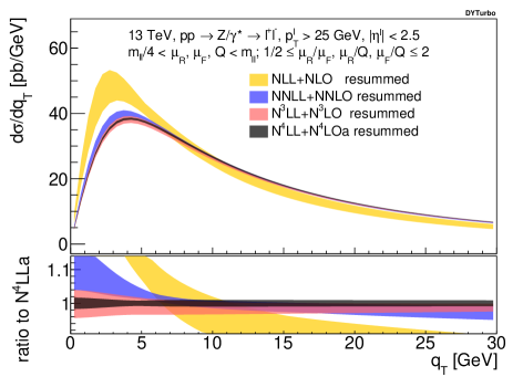
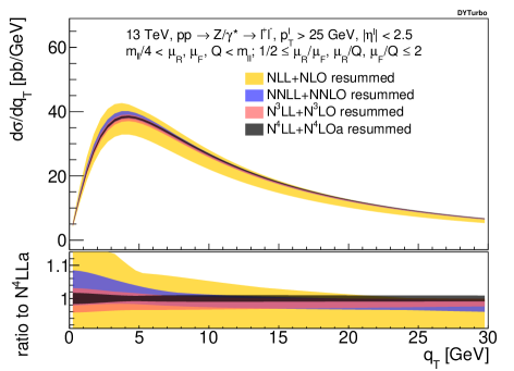
Figure 1: The $q_{T}$ spectrum of $Z/\gamma^{*}$ bosons with lepton selection cuts at the LHC ($\sqrt{s}=13$ TeV) at various perturbative orders. Resummed component (see Eq. (7)) of the hadronic cross-section with scale variation bands as defined in the text. The order of the parton density evolution is set consistently with the order of the resummation (left) or with the order of the PDFs (right).

In Fig. 1 we consider $Z/\gamma^{*}$ production and decay and we show the resummed component (see Eq. (7)) of the transverse-momentum distribution in the small-$q_{T}$ region. The label NⁿLL+NⁿLO ($n=1,2,3$) indicates that we perform the resummation of logarithmic enhanced contribution at NⁿLL accuracy including the hard-virtual coefficient at NⁿLO while the label N⁴LL+N⁴LOa indicate that we perform the resummation at N⁴LL accuracy with the hard-virtual coefficient at N⁴LO and an estimate of yet not known N⁴LO corrections .

In the left panel of Fig. 1 we show the resummed predictions following the original formalism of Refs. [6, 8, 17]. The lower panel shows the ratio of the distribution with respect to the N⁴LLa prediction at the central value of the scales $\mu_{F}=\mu_{R}=Q=M$. We observe that the NLL+NLO and NNLL+NNLO scale dependence bands do not overlap thus showing that the NLL+NLO scale variation underestimates the true perturbative uncertainty. This feature was already observed and discussed in Refs.[17, 48]. In the present case the lack of overlap can be ascribed to the fact that we are using the same N³LO parton densities set at NLL, NNLL, N³LL and N⁴LL accuracy. This choice introduce a formal mismatch between the N³LO Altarelli-Parisi evolution as encoded in the N³LO parton densities functions and the corresponding N^kLO evolution included in the N^k+1LL partonic resummed formula.

In order to show that this is indeed the case, in the right panel of Fig. 1 we show the resummed predictions in which we set the order of Altarelli-Parisi evolution in the resummed prediction to be equal to the order of the parton densities (i.e. both at approximated N³LO). In practice, with this choice, we are modifying the NLL, NNLL and N³LL predictions by including formally subleading logarithmic corrections . We observe that with this choice the scale dependence bands show a nice overlap at subsequent orders thus indicating that the lack of overlap of the previous case is indeed related to the mismatch in the order of the evolution of parton densities. However we also note that by keeping fixed the evolution of the parton densities at subsequent orders inevitably underestimates the impact of higher order corrections included in the PDFs.

Finally, we observe that the choice of the order in the the evolution of parton densities only affects the NLL+NLO and, with a minor extent, NNLO+NNLO theoretical predictions and corresponding uncertainties. Its impact is negligible at N³LL+N³LO (the N⁴LL+N⁴LOa prediction is independent by the choice). Since we are mainly interested on the impact of N⁴LL+N⁴LOa corrections with respect to the N³LL+N³LO results in the following we show numerical results only for the case in which the order of evolution of parton densities is set consistently with the order of the PDF set.

In both the left and right panel of Fig. 1 the scale dependence is consistently reduced increasing the perturbative order, in particular it is roughly reduced by a factor of 2 going from N³LL to N⁴LLa. The scale variation at N⁴LLa accuracy is around $\pm 1.5\%$ at $q_{T}\sim 1\,$GeV, then it reduces at $\pm 1\%$ level at the peak ($q_{T}\sim 4\,$GeV) and remains roughly constant up to $q_{T}\sim 30\,$GeV.

In the results of Fig. 1 we considered the effect of a finite top-quark mass including the singlet contributions mediated by heavy-quark loops at NNLO and N³LO. As already found in the literature [33, 34] the impact of these contribution is extremely small, the effect is of $-0.04\%$ at NNLO and less than $+0.001\%$ at N³LO.

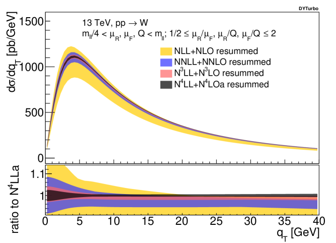
Figure 2: The $q_{T}$ spectrum of $W^{+}$ and $W^{-}$ bosons with inclusive leptonic decay at the LHC ($\sqrt{s}=13$ TeV) at various perturbative orders. Resummed component (see Eq. (7)) of the hadronic cross-section with scale variation bands as defined in the text.

In Fig. 2 we consider $W$ boson production and decay into a $l\nu_{l}$ pair showing the resummed component of the transverse-momentum distribution in the small-$q_{T}$ region at different perturbative orders. In this case we do not consider kinematical selection cuts apart a lower limit of $50$ GeV on the invariant mass of the vector boson (lepton pair) which is necessary in order to fix a hard scale for the process. Also in this case we observe that the scale dependence is consistently reduced increasing the perturbative order. The scale variation at N⁴LLa accuracy is around $\pm 2\%$ at $q_{T}\sim 1\,$GeV, then it reduces at $\pm 1\%$ level at the peak ($q_{T}\sim 4\,$GeV), it further decrease to $\pm 0.5\%$ for $q_{T}\sim 7\,$GeV and remains below $\pm 1\%$ level up to $q_{T}\sim 30\,$GeV.

The knowledge of the shape of the $W$ boson $q_{T}$ distribution and its uncertainty is particularly important since it affects the measurement of the $W$ mass. However the $W$ boson $q_{T}$ spectrum is not directly experimental accessible with good resolution due to the neutrino in final state of the leptonic $W$ decay. Conversely, the $q_{T}$ spectrum of the $Z$ boson has been measured with great precision. Therefore a precise theoretical prediction of the ratio of $W$ and $Z$ $q_{T}$ distributions, together with the measurement of the $Z$ boson $q_{T}$ spectrum, gives stringent information on the $W$ spectrum.

In Fig. 3 we consider the ratio of $q_{T}$ distributions for $Z/\gamma^{*}$ and $W^{\pm}$ production and decay. We consider the quantity

$$R(q_{T})=\frac{\sigma_{Z}}{\sigma_{W}}\,\frac{d\sigma_{W}}{dq_{T}}\Big{/}\frac{d\sigma_{Z}}{dq_{T}},$$ (4)

where $\frac{1}{\sigma_{V}}\,\frac{d\sigma_{V}}{dq_{T}}$ with $V=W,Z$ is the normalized $q_{T}$ distribution for $W$ and $Z/\gamma^{*}$ production and decay inclusive over the leptonic final state kinematics, apart for a selection cut on the invariant mass of the lepton pair: $80<M_{l^{+}l^{-}}<100\,$GeV and $M_{l\nu}>50\,$GeV.

In Fig. 3 we show the resummed component of the transverse-momentum distribution of Eq. 4 for the ratio $W^{+}/Z$ (left panel) and $W^{-}/Z$ (right panel) in the small-$q_{T}$ region. From the results of Fig. 3 (left and right panels) we observe that the scale dependence is greatly reduced (roughly by one order of magnitude) with respect to the distributions shown in Figs. 1,2. The scale variation at N⁴LL+N⁴LOa accuracy is around $\pm 0.3\%-0.4\%$ at $q_{T}\sim 1\,$GeV, then it reduces at $\pm 0.1\%$ level at the peak ($q_{T}\sim 4\,$GeV), it further decrease below $0.05\%$ level for $q_{T}\sim 7\,$GeV and then it slightly increase up to $\pm 0.2\%$ for $q_{T}\sim 30\,$GeV. This reduction of scale uncertainty is not unexpected because in the ratio correlated uncertainties on $W$ and $Z$ distributions cancel. In particular higher order QCD predictions for the resummed component of the cross section has a high degree of universalities and the process dependence is mainly due to the different flavour content of the partonic subprocesses for $W$ and $Z$ production.

One may wonder if correlated scale variation for the ratio of $W$ and $Z$ distribution can underestimate the true perturbative uncertainty. However the overlap of the scale uncertainty band indicates that correlated scale variation at NLL+NLO, NNLL+NNLO and N³LL+N³LO correctly estimate the size of higher-order corrections. An alternative, and more robust, perturbative uncertainty can be obtained considering the size of the difference between the prediction at a given order with respect to the prediction at the previous order. In this way we obtain an uncertainty which is even smaller than the one obtained through the perturbative scale variation method.

However we stress that the predictions presented in Fig. 3 are far from being complete since at such level of theoretical precision several effects cannot be neglected. In particular also very small effects which however are different in the $W$ and $Z$ case can give not negligible effects on the $W/Z$ ratio. For instance the impact of the process dependent finite component of the cross section, the (flavour dependent) non-perturbative intrinsic $k_{T}$ effects[55], the QED and electroweak effects [56, 57, 58, 59, 60], the heavy-quark mass effects [61, 62].

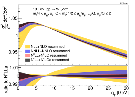
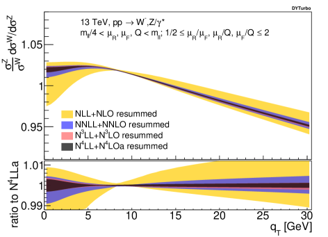
Figure 3: The normalized ratio of $q_{T}$ spectra of $W$ and $Z/\gamma^{*}$ bosons at the LHC ($\sqrt{s}=13$ TeV) at various perturbative orders for $W^{+}/Z$ (left) and $W^{-}/Z$ (right). Resummed component (see Eq. (7)) of the hadronic cross-section with scale variation bands as defined in the text.

In conclusion, in this paper we have presented the implementation of the $q_{T}$ resummation formalism of Refs. [6, 8, 17] for Drell–Yan processes up to N⁴LL+N⁴LO approximated accuracy in the DYTurbo numerical program [46, 47]. We have illustrated explicit numerical results for the resummed component of the transverse-momentum distribution for the case of $Z/\gamma^{*},W^{\pm}$ production and leptonic decay at LHC energies. We also considered theoretical predictions for the ratio of $W^{\pm}$ and $Z/\gamma^{*}$ $q_{T}$ distributions. Perturbative uncertainties have been estimated through a study of the scale variation band.

The DYTurbo numerical code allows the user to apply arbitrary kinematical cuts on the vector boson and the final-state leptons, and to compute the corresponding relevant distributions in the form of bin histograms. These features make the DYTurbo a useful tool for Drell–Yan studies at hadron colliders such as the Tevatron and the LHC.

Appendix A Transverse-momentum resummation up to N⁴LL+N⁴LO accuracy

We consider the process

$$h_{1}+h_{2}\to V+X\to l_{3}+l_{4}+X,$$ (5)

where $V$ denotes the vector boson produced by the colliding hadrons $h_{1}$ and $h_{2}$ with a centre–of–mass energy $s$, while $l_{3}$ and $l_{4}$ are the final state leptons produced by the $V$ decay. The lepton kinematics is completely specified in terms of the transverse-momentum ${\bf q_{T}}$ (with $q_{T}=\sqrt{{\bf q_{T}}^{2}}$), the rapidity $y$ and the invariant mass $M$ of the lepton pair, and by two additional variables ${\bf\Omega}$ that specify the angular distribution of the leptons with respect to the vector boson momentum.

We consider the Drell–Yan cross section fully differential in the leptonic final state. According to the factorization theorem we can write

$$\frac{d{\sigma}_{h_{1}h_{2}\to l_{3}l_{4}}}{d^{2}{\bf q_{T}}dM^{2}dyd\bf{\Omega}}({\bf q_{T}},M^{2},y,s,{\bf\Omega}) = \sum_{a_{1},a_{2}}\int_{0}^{1}dx_{1}\int_{0}^{1}dx_{2}\,f_{a_{1}/h_{1}}(x_{1},\mu_{F}^{2})\,f_{a_{2}/h_{2}}(x_{2},\mu_{F}^{2})$$ (6)

$$\times \,{\frac{d{\hat{\sigma}}_{a_{1}a_{2}\to l_{3}l_{4}}}{d^{2}{\bf q_{T}}\,d{M^{2}}\,d\hat{y}\,d{\bf\Omega}}}({\bf q_{T}},M,\hat{y},\hat{s},{\bf\Omega};\alpha_{S},\mu_{R}^{2},\mu_{F}^{2})\,,$$

where $f_{a/h}(x,\mu_{F}^{2})$ ($a=q_{f},\bar{q}_{f},g$) are the parton distribution functions of the hadron $h$, $\hat{s}=x_{1}x_{2}s$ is the partonic centre–of–mass energy squared, $\hat{y}=y-\ln\sqrt{x_{1}/x_{2}}$ is the vector boson rapidity with respect to the colliding partons while $\mu_{R}$ and $\mu_{F}$ are the renormalization and factorization scales. The last factor in the right-hand side of Eq. (6) is multi-differential partonic cross sections, computable in perturbative QCD as a series expansion in the strong coupling $\alpha_{S}=\alpha_{S}(\mu_{R})$, which will be denoted in the following by the shorthand notation $[d\hat{\sigma}_{a_{1}a_{2}\to l_{3}l_{4}}]$.

The partonic cross section can be decomposed as

$$[d\hat{\sigma}_{a_{1}a_{2}\to l_{3}l_{4}}]=[d\hat{\sigma}^{({\rm res.})}_{a_{1}a_{2}\to l_{3}l_{4}}]+[d\hat{\sigma}^{({\rm fin.})}_{a_{1}a_{2}\to l_{3}l_{4}}]$$ (7)

where the first term on the right-hand side of Eq. (7) is the resummed component which dominates in the small $q_{T}$ region while the second term is the finite component which is needed at large $q_{T}$.

We briefly review the impact-parameter space $b$ [4] resummation formalism of Refs. [6, 8, 17]. The resummed component in the r.h.s. of Eq. 7 can then be written as

$$\left[{d{\hat{\sigma}}_{a_{1}a_{2}\to l_{3}l_{4}}^{(\rm res.)}}\right]=\sum_{b_{1},b_{2}=q,{\bar{q}}}\!\!\frac{{d{\hat{\sigma}}^{(0)}_{b_{1}b_{2}\to l_{3}l_{4}}}}{d{\bf{\Omega}}}\;\frac{1}{\hat{s}}\;\int_{0}^{\infty}\frac{db}{2\pi}\;b\,J_{0}(bq_{T})\;{\cal W}_{a_{1}a_{2},b_{1}b_{2}\to V}(b,M,\hat{y},\hat{s};\alpha_{S},\mu_{R}^{2},\mu_{F}^{2})\;,$$ (8)

where $J_{0}(x)$ is the $0$th-order Bessel function and the factor $d{\hat{\sigma}}^{(0)}_{b_{1}b_{2}\to l_{3}l_{4}}$ is the Born level differential cross section for the partonic subprocess $q\bar{q}\to V\to l_{3}l_{4}$.

The function ${\cal W}_{V}(b,M,\hat{y},\hat{s})$ can be expressed in an exponential form by considering the ‘double’ $(N_{1},N_{2})$ Mellin moments with respect to the variables $z_{1}=e^{+\hat{y}}M/{\sqrt{\hat{s}}}$ and $z_{2}=e^{-\hat{y}}M/{\sqrt{\hat{s}}}$ at fixed $M$  [6, 63]

$${\cal W}_{V}(b,M;\alpha_{S},\mu_{R}^{2},\mu_{F}^{2})={\cal H}_{V}\left(\alpha_{S};M/\mu_{R},M/\mu_{F},M/Q\right)\times\exp\{{\cal G}(\alpha_{S},L;M/\mu_{R},M/Q)\}\,,$$ (9)

where we have introduced the logarithmic expansion parameter

$$L\equiv\ln({Q^{2}b^{2}}/{b_{0}^{2}})$$ (10)

with $b_{0}=2e^{-\gamma_{E}}$ ($\gamma_{E}=0.5772...$ is the Euler number). The scale $Q\sim M$ is the resummation scale [64], which parameterizes the arbitrariness in the resummation procedure.

The process dependent function ${\cal H}_{V}(\alpha_{S})$ [65, 66] includes the hard-collinear contributions and it can be written in term of a process dependent hard factor $H_{V}(\alpha_{S})$ and two process independent functions ${C}(\alpha_{S})$ associated to collinear emissions from the initial state colliding partons 

$${\cal H}_{V}(\alpha_{S})=H_{V}(\alpha_{S})\,{C}(\alpha_{S})\,{C}(\alpha_{S})\,.$$ (11)

The functions in Eq.(11) have a standard perturbative expansion

$${\cal H}_{V}(\alpha_{S}) = 1+\sum_{n=1}^{\infty}\left(\frac{\alpha_{S}}{\pi}\right)^{n}\,{\cal H}_{V}^{(n)},$$ (12)

$$H_{V}(\alpha_{S}) = 1+\sum_{n=1}^{\infty}\left(\frac{\alpha_{S}}{\pi}\right)^{n}\,{H}_{V}^{(n)},$$ (13)

$$C(\alpha_{S}) = 1+\sum_{n=1}^{\infty}\left(\frac{\alpha_{S}}{\pi}\right)^{n}\,{C}^{(n)}\,,$$ (14)

therefore up to the fourth order we have the following relations

$${\cal H}_{V}^{(1)} = {H}_{V}^{(1)}+{C}^{(1)}+{C}^{(1)},$$ (15)

$${\cal H}_{V}^{(2)} = {H}_{V}^{(2)}+{C}^{(2)}+{C}^{(2)}+{H}_{V}^{(1)}({C}^{(1)}+{C}^{(1)})+{C}^{(1)}{C}^{(1)},$$ (16)

$${\cal H}_{V}^{(3)} = {H}_{V}^{(3)}+{C}^{(3)}+{C}^{(3)}+{H}_{V}^{(2)}({C}^{(1)}+{C}^{(1)})+{H}_{V}^{(1)}({C}^{(2)}+{C}^{(2)}+{C}^{(1)}{C}^{(1)})$$ (17)

$$+ {C}^{(2)}{C}^{(1)}+{C}^{(2)}{C}^{(1)},$$

$${\cal H}_{V}^{(4)} = {H}_{V}^{(4)}+{C}^{(4)}+{C}^{(4)}+{H}_{V}^{(3)}({C}^{(1)}+{C}^{(1)})+{H}_{V}^{(2)}({C}^{(2)}+{C}^{(2)}+{C}^{(1)}{C}^{(1)})$$ (18)

$$+ {H}_{V}^{(1)}({C}^{(3)}+{C}^{(3)}+{C}^{(2)}{C}^{(1)}+{C}^{(2)}{C}^{(1)})+{C}^{(3)}{C}^{(1)}+{C}^{(3)}{C}^{(1)}+{C}^{(2)}{C}^{(2)}\,.$$

The universal (process independent) form factor $\exp\{{\cal G}\}$ in the right-hand side of Eq. (9) contains all the terms that order-by-order in $\alpha_{S}$ are logarithmically divergent as $b\to\infty$ (i.e. $q_{T}\to 0$). The resummed logarithmic expansion of ${\cal G}$ reads [6]

$${\cal G}(\alpha_{S},L) = -\int_{b_{0}^{2}/b^{2}}^{Q^{2}}\frac{dq^{2}}{q^{2}}\left[A(\alpha_{S}(q^{2}))\ln\frac{M^{2}}{q^{2}}+\widetilde{B}(\alpha_{S}(q^{2}))\right]$$ (19)

$$= L\,g^{(1)}(\alpha_{S}L)+g^{(2)}(\alpha_{S}L)+\sum_{n=1}^{\infty}\left(\frac{\alpha_{S}}{\pi}\right)^{n}\,{g}^{(n+2)}(\alpha_{S}L)\,,$$

where the functions $g^{(n)}$ control and resum the $\alpha_{S}^{k}L^{k}$ (with $k\geq 1$) logarithmic terms in the exponent of Eq. (9) due to soft and collinear radiation. The perturbative functions $A(\alpha_{S})$ and $\widetilde{B}(\alpha_{S})$ can be expanded as

$$A(\alpha_{S}) = \sum_{n=1}^{\infty}\left(\frac{\alpha_{S}}{\pi}\right)^{n}\,{A}^{(n)}\,,$$ (20)

$$\widetilde{B}(\alpha_{S}) = \sum_{n=1}^{\infty}\left(\frac{\alpha_{S}}{\pi}\right)^{n}\,{\widetilde{B}}^{(n)}\,.$$ (21)

The function $\widetilde{B}(\alpha_{S})$ can be written as follows

$$\widetilde{B}(\alpha_{S}) = B(\alpha_{S})+2\beta(\alpha_{S})\frac{d\ln C(\alpha_{S})}{d\ln\alpha_{S}}+2\gamma(\alpha_{S})\,,$$ (23)

in terms of the resummation coefficient $B(\alpha_{S})$, the collinear functions $C(\alpha_{S})$ (see Eq.(14)), the functions $\gamma(\alpha_{S})$ (the Mellin moments of the Altarelli–Parisi splitting functions ) and the QCD $\beta$ function

$$\frac{d\ln\alpha_{S}(\mu^{2})}{d\ln\mu^{2}}=\beta(\alpha_{S})=-\sum_{n=0}^{+\infty}\beta_{n}\left(\frac{\alpha_{S}}{\pi}\right)^{n+1}\,.$$ (24)

By explicit integration of Eq.(19) we obtain the following $g^{(i)}$ for $1\leq i\leq 5$

$$g^{(1)}(\alpha_{S}L) =\frac{A^{(1)}}{\beta_{0}}\frac{\lambda+\ln(1-\lambda)}{\lambda}\;\;,$$ (25)

$$g^{(2)}(\alpha_{S}L) =\frac{{\overline{B}}^{(1)}}{\beta_{0}}\ln(1-\lambda)-\frac{A^{(2)}}{\beta_{0}^{2}}\left(\frac{\lambda}{1-\lambda}+\ln(1-\lambda)\right)$$

$$+\frac{A^{(1)}}{\beta_{0}}\left(\frac{\lambda}{1-\lambda}+\ln(1-\lambda)\right)\ln\frac{Q^{2}}{\mu_{R}^{2}}$$

$$+\frac{A^{(1)}\beta_{1}}{\beta_{0}^{3}}\left(\frac{1}{2}\ln^{2}(1-\lambda)+\frac{\ln(1-\lambda)}{1-\lambda}+\frac{\lambda}{1-\lambda}\right)\;,$$ (26)

$$g^{(3)}(\alpha_{S}L) =-\frac{A^{(3)}}{2\beta_{0}^{2}}\frac{\lambda^{2}}{(1-\lambda)^{2}}-\frac{{\overline{B}}^{(2)}}{\beta_{0}}\frac{\lambda}{1-\lambda}+\frac{A^{(2)}\beta_{1}}{\beta_{0}^{3}}\left(\frac{\lambda(3\lambda-2)}{2(1-\lambda)^{2}}-\frac{(1-2\lambda)\ln(1-\lambda)}{(1-\lambda)^{2}}\right)$$

$$+\frac{{\overline{B}}^{(1)}\beta_{1}}{\beta_{0}^{2}}\left(\frac{\lambda}{1-\lambda}+\frac{\ln(1-\lambda)}{1-\lambda}\right)-\frac{A^{(1)}}{2}\frac{\lambda^{2}}{(1-\lambda)^{2}}\ln^{2}\frac{Q^{2}}{\mu_{R}^{2}}$$

$$+\ln\frac{Q^{2}}{\mu_{R}^{2}}\left({\overline{B}}^{(1)}\frac{\lambda}{1-\lambda}+\frac{A^{(2)}}{\beta_{0}}\frac{\lambda^{2}}{(1-\lambda)^{2}}+A^{(1)}\frac{\beta_{1}}{\beta_{0}^{2}}\left(\frac{\lambda}{1-\lambda}+\frac{1-2\lambda}{(1-\lambda)^{2}}\ln(1-\lambda)\right)\right)$$

$$+A^{(1)}\left(\frac{\beta_{1}^{2}}{2\beta_{0}^{4}}\frac{1-2\lambda}{(1-\lambda)^{2}}\ln^{2}(1-\lambda)+\ln(1-\lambda)\left[\frac{\beta_{0}\beta_{2}-\beta_{1}^{2}}{\beta_{0}^{4}}+\frac{\beta_{1}^{2}}{\beta_{0}^{4}(1-\lambda)}\right]\right.$$

$$\left.+\frac{\lambda}{2\beta_{0}^{4}(1-\lambda)^{2}}(\beta_{0}\beta_{2}(2-3\lambda)+\beta_{1}^{2}\lambda)\right)\;,$$ (27)

$$g^{(4)}(\alpha_{S}L) =-\frac{A^{(4)}}{6\beta_{0}^{2}}\frac{(3-\lambda)\lambda^{2}}{(1-\lambda)^{3}}-\frac{{\overline{B}}^{(3)}}{2\beta_{0}}\frac{(2-\lambda)\lambda}{(1-\lambda)^{2}}-\frac{A^{(3)}}{2\beta_{0}}\Bigg{(}\frac{\beta_{1}}{\beta_{0}^{2}}\bigg{[}\frac{(6-15\lambda+5\lambda^{2})\lambda}{6(1-\lambda)^{3}}\;\;$$

$$+\frac{(1-3\lambda)}{(1-\lambda)^{3}}\ln(1-\lambda)\bigg{]}-\frac{(3-\lambda)\lambda^{2}}{(1-\lambda)^{3}}\ln\frac{Q^{2}}{\mu_{R}^{2}}\Bigg{)}+{\overline{B}}^{(2)}\Bigg{(}\frac{\beta_{1}}{\beta_{0}^{2}}\bigg{[}\frac{(2-\lambda)\lambda}{2(1-\lambda)^{2}}+\frac{\ln(1-\lambda)}{(1-\lambda)^{2}}\bigg{]}\;\;$$

$$+\frac{(2-\lambda)\lambda}{(1-\lambda)^{2}}\ln\frac{Q^{2}}{\mu_{R}^{2}}\Bigg{)}+A^{(2)}\Bigg{(}-\frac{2\beta_{2}}{3\beta_{0}^{3}}\frac{\lambda^{3}}{(1-\lambda)^{3}}+\frac{\beta_{1}^{2}}{2\beta_{0}^{4}}\bigg{(}\frac{\lambda(6-9\lambda+11\lambda^{2})}{6(1-\lambda)^{3}}+\frac{\ln(1-\lambda)}{(1-\lambda)^{2}}\;\;$$

$$+\frac{1-3\lambda}{(1-\lambda)^{3}}\ln^{2}(1-\lambda)\bigg{)}+\bigg{[}\frac{\beta_{1}}{2\beta_{0}^{2}}\frac{(2-\lambda)\lambda}{(1-\lambda)^{2}}+\frac{\beta_{1}}{\beta_{0}^{2}}\frac{1-3\lambda}{(1-\lambda)^{3}}\ln(1-\lambda)\bigg{]}\ln\frac{Q^{2}}{\mu_{R}^{2}}\;\;$$

$$-\frac{(3-\lambda)\lambda^{2}}{2(1-\lambda)^{3}}\ln^{2}\frac{Q^{2}}{\mu_{R}^{2}}\Bigg{)}+{\overline{B}}^{(1)}\Bigg{(}\frac{\beta_{1}^{2}}{2\beta_{0}^{3}}\bigg{[}\frac{\lambda^{2}}{(1-\lambda)^{2}}-\frac{\ln^{2}(1-\lambda)}{(1-\lambda)^{2}}\bigg{]}-\frac{\beta_{2}}{2\beta_{0}^{2}}\frac{\lambda^{2}}{(1-\lambda)^{2}}\;\;$$

$$-\frac{\beta_{1}}{\beta_{0}}\frac{\ln(1-\lambda)}{(1-\lambda)^{2}}\ln\frac{Q^{2}}{\mu_{R}^{2}}-\frac{\beta_{0}}{2}\frac{(2-\lambda)\lambda}{(1-\lambda)^{2}}\,\ln^{2}\frac{Q^{2}}{\mu_{R}^{2}}\Bigg{)}+A^{(1)}\Bigg{(}-\frac{\beta_{1}^{3}}{\beta_{0}^{5}}\bigg{(}\frac{\lambda^{3}}{6(1-\lambda)^{3}}\;\;$$

$$+\frac{(1+\lambda)\lambda^{2}}{2(1-\lambda)^{3}}\ln(1-\lambda)+\frac{\lambda}{2(1-\lambda)^{3}}\ln^{2}(1-\lambda)+\frac{(1-3\lambda)}{6(1-\lambda)^{3}}\ln^{3}(1-\lambda)\bigg{)}\;\;$$

$$-\frac{\beta_{1}\beta_{2}}{2\beta_{0}^{4}}\bigg{(}\frac{\lambda(6-15\lambda+5\lambda^{2})}{6(1-\lambda)^{3}}+\frac{(1-3\lambda+2\lambda^{2}-2\lambda^{3})}{(1-\lambda)^{3}}\ln(1-\lambda)\bigg{)}\;\;$$

$$+\frac{\beta_{3}}{2\beta_{0}^{3}}\bigg{(}\frac{\lambda(6-15\lambda+7\lambda^{2})}{6(1-\lambda)^{3}}+\ln(1-\lambda)\bigg{)}+\Bigg{[}-\frac{\beta_{1}^{2}}{\beta_{0}^{3}}\bigg{(}\frac{\lambda^{2}(1+\lambda)}{2(1-\lambda)^{3}}+\frac{\lambda}{(1-\lambda)^{3}}\ln(1-\lambda)\;\;$$

$$+\frac{1-3\lambda}{2(1-\lambda)^{3}}\ln^{2}(1-\lambda)\bigg{)}+\frac{\beta_{2}}{2\beta_{0}^{2}}\frac{\lambda^{2}(1+\lambda)}{(1-\lambda)^{3}}\Bigg{]}\ln\frac{Q^{2}}{\mu_{R}^{2}}-\frac{\beta_{1}}{2\beta_{0}}\Bigg{[}\frac{\lambda}{(1-\lambda)^{3}}\;\;$$

$$+\frac{1-3\lambda}{(1-\lambda)^{3}}\ln(1-\lambda)\Bigg{]}\ln^{2}\frac{Q^{2}}{\mu_{R}^{2}}+\frac{\beta_{0}}{6}\frac{(3-\lambda)\lambda^{2}}{(1-\lambda)^{3}}\ln^{3}\frac{Q^{2}}{\mu_{R}^{2}}\Bigg{)}\;,$$ (28)

$$g^{(5)}(\alpha_{S}L) =-\frac{A^{(5)}}{12\beta_{0}^{2}}\frac{\lambda^{2}(6-4\lambda+\lambda^{2})}{(1-\lambda)^{4}}-\frac{{\overline{B}}^{(4)}}{3\beta_{0}}\frac{\lambda(3-3\lambda+\lambda^{2})}{(1-\lambda)^{3}}\;\;$$

$$+\frac{A^{(4)}}{3\beta_{0}}\Bigg{(}\frac{\beta_{1}}{\beta_{0}^{2}}\Bigg{[}\frac{\lambda(-12+42\lambda-28\lambda^{2}+7\lambda^{3})}{12(1-\lambda)^{4}}-\frac{1-4\lambda}{(1-\lambda)^{4}}\ln(1-\lambda)\Bigg{]}\;\;$$

$$+\frac{\lambda^{2}(6-4\lambda+\lambda^{2})}{(1-\lambda)^{4}}\ln\frac{Q^{2}}{\mu_{R}^{2}}\Bigg{)}+{\overline{B}}^{(3)}\Bigg{(}\frac{\beta_{1}}{\beta_{0}^{2}}\Bigg{[}\frac{\lambda(3-3\lambda+\lambda^{2})}{3(1-\lambda)^{3}}+\frac{\ln(1-\lambda)}{(1-\lambda)^{3}}\Bigg{]}\;\;$$

$$+\frac{\lambda(3-3\lambda+\lambda^{2})}{(1-\lambda)^{3}}\ln\frac{Q^{2}}{\mu_{R}^{2}}\Bigg{)}+A^{(3)}\Bigg{(}-\frac{\beta_{2}}{4\beta_{0}^{3}}\frac{\lambda^{3}(4-\lambda)}{(1-\lambda)^{4}}\;\;$$

$$+\frac{\beta_{1}^{2}}{\beta_{0}^{4}}\Bigg{[}\frac{\lambda(12-24\lambda+52\lambda^{2}-13\lambda^{3})}{36(1-\lambda)^{4}}+\frac{\ln(1-\lambda)}{3(1-\lambda)^{3}}+\frac{1-4\lambda}{2(1-\lambda)^{4}}\ln^{2}(1-\lambda)\Bigg{]}\;\;$$

$$+\frac{\beta_{1}}{\beta_{0}^{2}}\Bigg{[}\frac{\lambda(3-3\lambda+\lambda^{2})}{3(1-\lambda)^{3}}+\frac{1-4\lambda}{(1-\lambda)^{4}}\ln(1-\lambda)\Bigg{]}\ln\frac{Q^{2}}{\mu_{R}^{2}}\;\;$$

$$-\frac{\lambda^{2}(6-4\lambda+\lambda^{2})}{2(1-\lambda)^{4}}\ln^{2}\frac{Q^{2}}{\mu_{R}^{2}}\Bigg{)}+{\overline{B}}^{(2)}\Bigg{(}-\frac{\beta_{2}}{3\beta_{0}^{2}}\frac{(3-\lambda)\lambda^{2}}{(1-\lambda)^{3}}+\frac{\beta_{1}^{2}}{\beta_{0}^{3}}\bigg{(}\frac{(3-\lambda)\lambda^{2}}{3(1-\lambda)^{3}}\;\;$$

$$-\frac{\ln^{2}(1-\lambda)}{(1-\lambda)^{3}}\bigg{)}-\frac{2\beta_{1}}{\beta_{0}}\frac{\ln(1-\lambda)}{(1-\lambda)^{3}}\ln\frac{Q^{2}}{\mu_{R}^{2}}-\beta_{0}\frac{\lambda(3-3\lambda+\lambda^{2})}{(1-\lambda)^{3}}\ln^{2}\frac{Q^{2}}{\mu_{R}^{2}}\Bigg{)}\;\;$$

$$+A^{(2)}\Bigg{(}-\frac{\beta_{3}}{12\beta_{0}^{3}}\frac{\lambda^{3}(8-5\lambda)}{(1-\lambda)^{4}}+\frac{\beta_{1}\beta_{2}}{3\beta_{0}^{4}}\bigg{(}\frac{\lambda(6-21\lambda+44\lambda^{2}-20\lambda^{3})}{6(1-\lambda)^{4}}\;\;$$

$$+\frac{1-4\lambda+9\lambda^{2}}{(1-\lambda)^{4}}\ln(1-\lambda)\bigg{)}+\frac{\beta_{1}^{3}}{\beta_{0}^{5}}\bigg{(}\frac{\lambda(-12+42\lambda-64\lambda^{2}+25\lambda^{3})}{36(1-\lambda)^{4}}\;\;$$

$$-\frac{(1-4\lambda+9\lambda^{2})}{3(1-\lambda)^{4}}\ln(1-\lambda)-\frac{\lambda}{(1-\lambda)^{4}}\ln^{2}(1-\lambda)-\frac{1-4\lambda}{3(1-\lambda)^{4}}\ln^{3}(1-\lambda)\bigg{)}\;\;$$

$$+\Bigg{[}\frac{\beta_{2}}{3\beta_{0}^{2}}\frac{(3+4\lambda-\lambda^{2})\lambda^{2}}{(1-\lambda)^{4}}+\frac{\beta_{1}^{2}}{\beta_{0}^{3}}\bigg{(}-\frac{(3+4\lambda-\lambda^{2})\lambda^{2}}{3(1-\lambda)^{4}}-\frac{2\lambda}{(1-\lambda)^{4}}\ln(1-\lambda)\;\;$$

$$-\frac{1-4\lambda}{(1-\lambda)^{4}}\ln^{2}(1-\lambda)\bigg{)}\Bigg{]}\ln\frac{Q^{2}}{\mu_{R}^{2}}+\frac{\beta_{1}}{\beta_{0}}\Bigg{[}-\frac{\lambda}{(1-\lambda)^{4}}-\frac{1-4\lambda}{(1-\lambda)^{4}}\ln(1-\lambda)\Bigg{]}\ln^{2}\frac{Q^{2}}{\mu_{R}^{2}}\;\;$$

$$+\frac{\beta_{0}}{3}\frac{\lambda^{2}(6-4\lambda+\lambda^{2})}{(1-\lambda)^{4}}\ln^{3}\frac{Q^{2}}{\mu_{R}^{2}}\Bigg{)}+{\overline{B}}^{(1)}\Bigg{(}-\frac{\beta_{3}}{6\beta_{0}^{2}}\frac{(3-2\lambda)\lambda^{2}}{(1-\lambda)^{3}}+\frac{\beta_{1}\beta_{2}}{\beta_{0}^{3}}\bigg{(}\frac{(3-2\lambda)\lambda^{2}}{3(1-\lambda)^{3}}\;\;$$

$$+\frac{\lambda}{(1-\lambda)^{3}}\ln(1-\lambda)\bigg{)}+\frac{\beta_{1}^{3}}{\beta_{0}^{4}}\bigg{(}-\frac{(3-2\lambda)\lambda^{2}}{6(1-\lambda)^{3}}-\frac{\lambda}{(1-\lambda)^{3}}\ln(1-\lambda)-\frac{\ln^{2}(1-\lambda)}{2(1-\lambda)^{3}}\;\;$$

$$+\frac{\ln^{3}(1-\lambda)}{3(1-\lambda)^{3}}\bigg{)}+\Bigg{[}\frac{\beta_{2}}{\beta_{0}}\frac{\lambda}{(1-\lambda)^{3}}+\frac{\beta_{1}^{2}}{\beta_{0}^{2}}\bigg{(}-\frac{\lambda}{(1-\lambda)^{3}}-\frac{\ln(1-\lambda)}{(1-\lambda)^{3}}+\frac{\ln^{2}(1-\lambda)}{(1-\lambda)^{3}}\bigg{)}\Bigg{]}\ln\frac{Q^{2}}{\mu_{R}^{2}}\;\;$$

$$+\beta_{1}\Bigg{[}-\frac{\lambda(3-3\lambda+\lambda^{2})}{2(1-\lambda)^{3}}+\frac{\ln(1-\lambda)}{(1-\lambda)^{3}}\Bigg{]}\ln^{2}\frac{Q^{2}}{\mu_{R}^{2}}+\beta_{0}^{2}\frac{\lambda(3-3\lambda+\lambda^{2})}{3(1-\lambda)^{3}}\ln^{3}\frac{Q^{2}}{\mu_{R}^{2}}\Bigg{)}\;\;$$

$$+A^{(1)}\Bigg{(}\frac{\beta_{2}^{2}}{3\beta_{0}^{4}}\bigg{(}\frac{\lambda(-12+42\lambda-52\lambda^{2}+7\lambda^{3})}{12(1-\lambda)^{4}}-\ln(1-\lambda)\bigg{)}\;\;$$

$$+\frac{\beta_{4}}{3\beta_{0}^{3}}\bigg{(}\frac{\lambda(12-42\lambda+40\lambda^{2}-13\lambda^{3})}{12(1-\lambda)^{4}}+\ln(1-\lambda)\bigg{)}+\frac{\beta_{1}\beta_{3}}{6\beta_{0}^{4}}\bigg{(}-\frac{\lambda(2-5\lambda)}{3}\frac{(3-3\lambda+\lambda^{2})}{(1-\lambda)^{4}}\;\;$$

$$-\frac{2-8\lambda+9\lambda^{2}-10\lambda^{3}+4\lambda^{4}}{(1-\lambda)^{4}}\ln(1-\lambda)\bigg{)}+\frac{\beta_{1}^{2}\beta_{2}}{\beta_{0}^{5}}\bigg{(}\frac{\lambda(12-42\lambda+52\lambda^{2}+5\lambda^{3})}{36(1-\lambda)^{4}}\;\;$$

$$-\frac{(-1+3\lambda-3\lambda^{2}+3\lambda^{3})}{3(1-\lambda)^{3}}\ln(1-\lambda)-\frac{3\lambda^{2}}{2(1-\lambda)^{4}}\ln^{2}(1-\lambda)\bigg{)}+\frac{\beta_{1}^{4}}{2\beta_{0}^{6}}\bigg{(}-\frac{\lambda^{3}(2+3\lambda)}{6(1-\lambda)^{4}}\;\;$$

$$+\frac{\lambda^{2}(-3+2\lambda-2\lambda^{2})}{3(1-\lambda)^{4}}\ln(1-\lambda)-\frac{(1-3\lambda)\lambda}{(1-\lambda)^{4}}\ln^{2}(1-\lambda)-\frac{1-6\lambda}{3(1-\lambda)^{4}}\ln^{3}(1-\lambda)\;\;$$

$$+\frac{1-4\lambda}{6(1-\lambda)^{4}}\ln^{4}(1-\lambda)\bigg{)}+\Bigg{[}-\frac{\beta_{3}}{6\beta_{0}^{2}}\frac{\lambda^{2}(-3-2\lambda+2\lambda^{2})}{(1-\lambda)^{4}}-\frac{\beta_{1}\beta_{2}}{\beta_{0}^{3}}\bigg{(}\frac{2\lambda^{3}}{3(1-\lambda)^{3}}+\frac{3\lambda^{2}}{(1-\lambda)^{4}}\ln(1-\lambda)\bigg{)}\;\;$$

$$+\frac{\beta_{1}^{3}}{\beta_{0}^{4}}\bigg{(}-\frac{\lambda^{2}(3-2\lambda+2\lambda^{2})}{6(1-\lambda)^{4}}-\frac{(1-3\lambda)\lambda}{(1-\lambda)^{4}}\ln(1-\lambda)-\frac{1-6\lambda}{2(1-\lambda)^{4}}\ln^{2}(1-\lambda)\;\;$$

$$+\frac{1-4\lambda}{3(1-\lambda)^{4}}\ln^{3}(1-\lambda)\bigg{)}\Bigg{]}\ln\frac{Q^{2}}{\mu_{R}^{2}}+\Bigg{[}-\frac{3\beta_{2}}{2\beta_{0}}\frac{\lambda^{2}}{(1-\lambda)^{4}}+\frac{\beta_{1}^{2}}{2\beta_{0}^{2}}\bigg{(}-\frac{(1-3\lambda)\lambda}{(1-\lambda)^{4}}-\frac{(1-6\lambda)}{(1-\lambda)^{4}}\ln(1-\lambda)\;\;$$

$$+\frac{(1-4\lambda)}{(1-\lambda)^{4}}\ln^{2}(1-\lambda)\bigg{)}\Bigg{]}\ln^{2}\frac{Q^{2}}{\mu_{R}^{2}}+\frac{\beta_{1}}{3}\Bigg{[}\frac{\lambda(2+6\lambda-4\lambda^{2}+\lambda^{3})}{2(1-\lambda)^{4}}+\frac{1-4\lambda}{(1-\lambda)^{4}}\ln(1-\lambda)\Bigg{]}\ln^{3}\frac{Q^{2}}{\mu_{R}^{2}}\;\;$$

$$-\frac{\beta_{0}^{2}}{12}\frac{(6-4\lambda+\lambda^{2})\lambda^{2}}{(1-\lambda)^{4}}\ln^{4}\frac{Q^{2}}{\mu_{R}^{2}}\Bigg{)}\;,$$ (29)

where

$$\lambda=\frac{1}{\pi}\,\beta_{0}\,\alpha_{S}(\mu_{R}^{2})\,L\;\;,$$ (30)

$${\overline{B}}^{(n)}={\widetilde{B}}^{(n)}+A^{(n)}\ln\frac{M^{2}}{Q^{2}}\;\;.$$ (31)

The $g^{(1)}$, $g^{(2)}$ and $g^{(3)}$ resummation functions can be found in Ref. [6]. The $g^{(4)}$ function can be found in Ref. [67] for the related case of direct transverse momentum space resummation. The explicit expression of the first five coefficients of the $\beta$ function, can be found in the following references: $\beta_{0}$, $\beta_{1}$ and $\beta_{2}$ in Refs. [68, 69], $\beta_{3}$ in Ref. [70] and $\beta_{4}$ in [71].

At NLL+NLO we include the functions $g^{(1)}$, $g^{(2)}$ and ${\cal H}_{V}^{(1)}$, at NNLL+NNLO we also include the functions $g^{(3)}$ and ${\cal H}_{V}^{(2)}$ [72, 73], at N³LL+N³LO the functions $g^{(4)}$ and ${\cal H}_{V}^{(3)}$  [74, 75] and finally at N⁴LL+N³LO the function $g^{(5)}$ and ${\cal H}_{V}^{(4)}$.

We consider uncertainties in the numerical approximations of the N⁴LL coefficients, and estimate uncertainties arising from the incomplete knowledge of the N⁴LO perturbative coefficients. The $B^{(4)}$ coefficient and the non-singlet four-loop splitting functions are known with good numerical approximation [76, 77, 78], the corresponding relative uncertainties on the $q_{T}$ distribution are at the level of $10^{-6}$ or smaller, and considered negligible. The numerical approximations of $A^{(5)}$ [79, 80, 81, 82, 83, 84, 85] and of the 4-loop singlet splitting functions [86, 87] are the dominant uncertainties in the N⁴LL approximation, and they amount to $1$–$3\cdot 10^{-3}$ relative uncertainty. In order to estimate the size of the unknown the $C^{(4)}$ coefficients [88] we perform a Levin transform of the corresponding perturbative series [89, 90] to guess the value of the fourth term in these series, and assign to it a $100\%$ uncertainty. This is equivalent to assuming that the Levin transform is able to estimate the sign and the order of magnitude of these unknown coefficients. The corresponding uncertainty is at the level of $1$–$2\cdot 10^{-3}$, and affects mostly the overall normalization. The uncertainties in the N⁴LL+N⁴LO approximation are shown in Fig. 4, and found to be 5 to 10 times smaller compared to the missing higher order uncertainties estimated through scale variations.

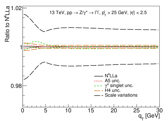
Figure 4: Uncertainties arising from numerical approximations or incomplete knowledge of the perturbative coefficients at N⁴LL+N⁴LOa, compared to missing higher order uncertainties estimated with scale variations at this order.

References

- [1] S. D. Drell and Tung-Mow Yan. Massive Lepton Pair Production in Hadron-Hadron Collisions at High-Energies. Phys. Rev. Lett., 25:316–320, 1970. [Erratum: Phys.Rev.Lett. 25, 902 (1970)].
- [2] J. H. Christenson, G. S. Hicks, L. M. Lederman, P. J. Limon, B. G. Pope, and E. Zavattini. Observation of massive muon pairs in hadron collisions. Phys. Rev. Lett., 25:1523–1526, Nov 1970.
- [3] Yuri L. Dokshitzer, Dmitri Diakonov, and S. I. Troian. On the Transverse Momentum Distribution of Massive Lepton Pairs. Phys. Lett. B, 79:269–272, 1978.
- [4] G. Parisi and R. Petronzio. Small Transverse Momentum Distributions in Hard Processes. Nucl. Phys. B, 154:427–440, 1979.
- [5] John C. Collins, Davison E. Soper, and George F. Sterman. Transverse Momentum Distribution in Drell-Yan Pair and W and Z Boson Production. Nucl. Phys. B, 250:199–224, 1985.
- [6] Giuseppe Bozzi, Stefano Catani, Daniel de Florian, and Massimiliano Grazzini. Transverse-momentum resummation and the spectrum of the Higgs boson at the LHC. Nucl. Phys. B, 737:73–120, 2006.
- [7] Giuseppe Bozzi, Stefano Catani, Giancarlo Ferrera, Daniel de Florian, and Massimiliano Grazzini. Transverse-momentum resummation: A Perturbative study of Z production at the Tevatron. Nucl. Phys. B, 815:174–197, 2009.
- [8] Giuseppe Bozzi, Stefano Catani, Giancarlo Ferrera, Daniel de Florian, and Massimiliano Grazzini. Production of Drell-Yan lepton pairs in hadron collisions: Transverse-momentum resummation at next-to-next-to-leading logarithmic accuracy. Phys. Lett. B, 696:207–213, 2011.
- [9] Stefano Catani and Massimiliano Grazzini. QCD transverse-momentum resummation in gluon fusion processes. Nucl. Phys. B, 845:297–323, 2011.
- [10] Thomas Becher and Matthias Neubert. Drell-Yan Production at Small , Transverse Parton Distributions and the Collinear Anomaly. Eur. Phys. J. C, 71:1665, 2011.
- [11] Thomas Becher, Matthias Neubert, and Daniel Wilhelm. Electroweak Gauge-Boson Production at Small : Infrared Safety from the Collinear Anomaly. JHEP, 02:124, 2012.
- [12] John Collins. Foundations of perturbative QCD. Camb. Monogr. Part. Phys. Nucl. Phys. Cosmol., 32:1–624, 2011.
- [13] John C. Collins and Ted C. Rogers. Equality of Two Definitions for Transverse Momentum Dependent Parton Distribution Functions. Phys. Rev. D, 87(3):034018, 2013.
- [14] Andrea Banfi, Mrinal Dasgupta, Simone Marzani, and Lee Tomlinson. Predictions for Drell-Yan and observables at the LHC. Phys. Lett., B715:152–156, 2012.
- [15] Marco Guzzi, Pavel M. Nadolsky, and Bowen Wang. Nonperturbative contributions to a resummed leptonic angular distribution in inclusive neutral vector boson production. Phys. Rev. D, 90(1):014030, 2014.
- [16] John Collins and Ted Rogers. Understanding the large-distance behavior of transverse-momentum-dependent parton densities and the Collins-Soper evolution kernel. Phys. Rev. D, 91(7):074020, 2015.
- [17] Stefano Catani, Daniel de Florian, Giancarlo Ferrera, and Massimiliano Grazzini. Vector boson production at hadron colliders: transverse-momentum resummation and leptonic decay. JHEP, 12:047, 2015.
- [18] Markus A. Ebert and Frank J. Tackmann. Resummation of Transverse Momentum Distributions in Distribution Space. JHEP, 02:110, 2017.
- [19] Francesco Coradeschi and Thomas Cridge. reSolve — A transverse momentum resummation tool. Comput. Phys. Commun., 238:262–294, 2019.
- [20] Ignazio Scimemi and Alexey Vladimirov. Analysis of vector boson production within TMD factorization. Eur. Phys. J. C, 78(2):89, 2018.
- [21] Wojciech Bizoń, Xuan Chen, Aude Gehrmann-De Ridder, Thomas Gehrmann, Nigel Glover, Alexander Huss, Pier Francesco Monni, Emanuele Re, Luca Rottoli, and Paolo Torrielli. Fiducial distributions in Higgs and Drell-Yan production at N3LL+NNLO. JHEP, 12:132, 2018.
- [22] Wojciech Bizon, Aude Gehrmann-De Ridder, Thomas Gehrmann, Nigel Glover, Alexander Huss, Pier Francesco Monni, Emanuele Re, Luca Rottoli, and Duncan M. Walker. The transverse momentum spectrum of weak gauge bosons at N3LLNNLO. 2019.
- [23] Thomas Becher and Monika Hager. Event-Based Transverse Momentum Resummation. 2019.
- [24] Valerio Bertone, Ignazio Scimemi, and Alexey Vladimirov. Extraction of unpolarized quark transverse momentum dependent parton distributions from Drell-Yan/Z-boson production. JHEP, 06:028, 2019.
- [25] Alessandro Bacchetta, Valerio Bertone, Chiara Bissolotti, Giuseppe Bozzi, Filippo Delcarro, Fulvio Piacenza, and Marco Radici. Transverse-momentum-dependent parton distributions up to N3LL from Drell-Yan data. JHEP, 07:117, 2020.
- [26] Markus A. Ebert, Johannes K. L. Michel, Iain W. Stewart, and Frank J. Tackmann. Drell-Yan Resummation of Fiducial Power Corrections at N3LL. 6 2020.
- [27] Thomas Becher and Tobias Neumann. Fiducial resummation of color-singlet processes at N3LL+NNLO. 9 2020.
- [28] Emanuele Re, Luca Rottoli, and Paolo Torrielli. Fiducial Higgs and Drell-Yan distributions at N3LL′+NNLO with RadISH. 4 2021.
- [29] Simone Alioli, Christian W. Bauer, Alessandro Broggio, Alessandro Gavardi, Stefan Kallweit, Matthew A. Lim, Riccardo Nagar, Davide Napoletano, and Luca Rottoli. Matching NNLO to parton shower using N3LL colour-singlet transverse momentum resummation in GENEVA. 2 2021.
- [30] Wan-Li Ju and Marek Schönherr. The qT and spectra in W and Z production at the LHC at N3LL’+N2LO. JHEP, 10:088, 2021.
- [31] Tobias Neumann and John Campbell. Fiducial Drell-Yan production at the LHC improved by transverse-momentum resummation at N4LLp+N3LO. Phys. Rev. D, 107(1):L011506, 2023.
- [32] Xuan Chen, Thomas Gehrmann, E. W. N. Glover, Alexander Huss, Pier Francesco Monni, Emanuele Re, Luca Rottoli, and Paolo Torrielli. Third-Order Fiducial Predictions for Drell-Yan Production at the LHC. Phys. Rev. Lett., 128(25):252001, 2022.
- [33] Duane A. Dicus and Scott S. D. Willenbrock. Radiative Corrections to the Ratio of and Boson Production. Phys. Rev. D, 34:148, 1986.
- [34] P. J. Rijken and W. L. van Neerven. Heavy flavor contributions to the Drell-Yan cross-section. Phys. Rev. D, 52:149–161, 1995.
- [35] Long Chen, Michał Czakon, and Marco Niggetiedt. The complete singlet contribution to the massless quark form factor at three loops in QCD. JHEP, 12:095, 2021.
- [36] R. N. Lee, A. V. Smirnov, and V. A. Smirnov. Analytic Results for Massless Three-Loop Form Factors. JHEP, 04:020, 2010.
- [37] T. Gehrmann, E. W. N. Glover, T. Huber, N. Ikizlerli, and C. Studerus. Calculation of the quark and gluon form factors to three loops in QCD. JHEP, 06:094, 2010.
- [38] Radja Boughezal, Christfried Focke, Xiaohui Liu, and Frank Petriello. -boson production in association with a jet at next-to-next-to-leading order in perturbative QCD. Phys. Rev. Lett., 115(6):062002, 2015.
- [39] A. Gehrmann-De Ridder, T. Gehrmann, E. W. N. Glover, A. Huss, and T. A. Morgan. Precise QCD predictions for the production of a Z boson in association with a hadronic jet. Phys. Rev. Lett., 117(2):022001, 2016.
- [40] Radja Boughezal, John M. Campbell, R. Keith Ellis, Christfried Focke, Walter T. Giele, Xiaohui Liu, and Frank Petriello. Z-boson production in association with a jet at next-to-next-to-leading order in perturbative QCD. Phys. Rev. Lett., 116(15):152001, 2016.
- [41] Radja Boughezal, Xiaohui Liu, and Frank Petriello. W-boson plus jet differential distributions at NNLO in QCD. Phys. Rev. D, 94(11):113009, 2016.
- [42] Radja Boughezal, Xiaohui Liu, and Frank Petriello. Phenomenology of the Z-boson plus jet process at NNLO. Phys. Rev. D, 94(7):074015, 2016.
- [43] Aude Gehrmann-De Ridder, T. Gehrmann, E. W. N. Glover, A. Huss, and T. A. Morgan. The NNLO QCD corrections to Z boson production at large transverse momentum. JHEP, 07:133, 2016.
- [44] A. Gehrmann-De Ridder, T. Gehrmann, E. W. N. Glover, A. Huss, and T. A. Morgan. NNLO QCD corrections for Drell-Yan and observables at the LHC. JHEP, 11:094, 2016. [Erratum: JHEP 10, 126 (2018)].
- [45] A. Gehrmann-De Ridder, T. Gehrmann, E. W. N. Glover, A. Huss, and D. M. Walker. Next-to-Next-to-Leading-Order QCD Corrections to the Transverse Momentum Distribution of Weak Gauge Bosons. Phys. Rev. Lett., 120(12):122001, 2018.
- [46] Stefano Camarda et al. DYTurbo: Fast predictions for Drell-Yan processes. Eur. Phys. J. C, 80(3):251, 2020. [Erratum: Eur.Phys.J.C 80, 440 (2020)].
- [47] Stefano Camarda et al. https://dyturbo.hepforge.org/.
- [48] Stefano Camarda, Leandro Cieri, and Giancarlo Ferrera. Drell–Yan lepton-pair production: qT resummation at N3LL accuracy and fiducial cross sections at N3LO. Phys. Rev. D, 104(11):L111503, 2021.
- [49] J. McGowan, T. Cridge, L. A. Harland-Lang, and R. S. Thorne. Approximate N3LO parton distribution functions with theoretical uncertainties: MSHT20aN3LO PDFs. Eur. Phys. J. C, 83(3):185, 2023.
- [50] John C. Collins and Davison E. Soper. Angular Distribution of Dileptons in High-Energy Hadron Collisions. Phys. Rev. D, 16:2219, 1977.
- [51] John C. Collins and Davison E. Soper. Back-To-Back Jets: Fourier Transform from B to K-Transverse. Nucl. Phys. B, 197:446–476, 1982.
- [52] Stefano Catani, Michelangelo L. Mangano, Paolo Nason, and Luca Trentadue. The Resummation of soft gluons in hadronic collisions. Nucl. Phys. B, 478:273–310, 1996.
- [53] Eric Laenen, George F. Sterman, and Werner Vogelsang. Higher order QCD corrections in prompt photon production. Phys. Rev. Lett., 84:4296–4299, 2000.
- [54] Anna Kulesza, George F. Sterman, and Werner Vogelsang. Joint resummation in electroweak boson production. Phys. Rev. D, 66:014011, 2002.
- [55] Andrea Signori, Alessandro Bacchetta, Marco Radici, and Gunar Schnell. Investigations into the flavor dependence of partonic transverse momentum. JHEP, 11:194, 2013.
- [56] Luca Barze, Guido Montagna, Paolo Nason, Oreste Nicrosini, and Fulvio Piccinini. Implementation of electroweak corrections in the POWHEG BOX: single W production. JHEP, 04:037, 2012.
- [57] Luca Barze, Guido Montagna, Paolo Nason, Oreste Nicrosini, Fulvio Piccinini, and Alessandro Vicini. Neutral current Drell-Yan with combined QCD and electroweak corrections in the POWHEG BOX. Eur. Phys. J. C, 73(6):2474, 2013.
- [58] S. Alioli et al. Precision studies of observables in and processes at the LHC. Eur. Phys. J. C, 77(5):280, 2017.
- [59] Leandro Cieri, Giancarlo Ferrera, and German F. R. Sborlini. Combining QED and QCD transverse-momentum resummation for Z boson production at hadron colliders. JHEP, 08:165, 2018.
- [60] Andrea Autieri, Leandro Cieri, Giancarlo Ferrera, and German F. R. Sborlini. Combining QED and QCD transverse-momentum resummation for W and Z boson production at hadron colliders. 2 2023.
- [61] Emanuele Bagnaschi, Fabio Maltoni, Alessandro Vicini, and Marco Zaro. Lepton-pair production in association with a pair and the determination of the boson mass. JHEP, 07:101, 2018.
- [62] Piotr Pietrulewicz, Daniel Samitz, Anne Spiering, and Frank J. Tackmann. Factorization and Resummation for Massive Quark Effects in Exclusive Drell-Yan. JHEP, 08:114, 2017.
- [63] Giuseppe Bozzi, Stefano Catani, Daniel de Florian, and Massimiliano Grazzini. Higgs boson production at the LHC: Transverse-momentum resummation and rapidity dependence. Nucl. Phys. B, 791:1–19, 2008.
- [64] G. Bozzi, S. Catani, D. de Florian, and M. Grazzini. The q(T) spectrum of the Higgs boson at the LHC in QCD perturbation theory. Phys. Lett. B, 564:65–72, 2003.
- [65] Stefano Catani, Daniel de Florian, and Massimiliano Grazzini. Universality of nonleading logarithmic contributions in transverse momentum distributions. Nucl. Phys. B, 596:299–312, 2001.
- [66] Stefano Catani, Leandro Cieri, Daniel de Florian, Giancarlo Ferrera, and Massimiliano Grazzini. Universality of transverse-momentum resummation and hard factors at the NNLO. Nucl. Phys. B, 881:414–443, 2014.
- [67] Wojciech Bizon, Pier Francesco Monni, Emanuele Re, Luca Rottoli, and Paolo Torrielli. Momentum-space resummation for transverse observables and the Higgs p⟂ at N3LL+NNLO. JHEP, 02:108, 2018.
- [68] O. V. Tarasov, A. A. Vladimirov, and A. Yu. Zharkov. The Gell-Mann-Low Function of QCD in the Three Loop Approximation. Phys. Lett. B, 93:429–432, 1980.
- [69] S. A. Larin and J. A. M. Vermaseren. The Three loop QCD Beta function and anomalous dimensions. Phys. Lett. B, 303:334–336, 1993.
- [70] T. van Ritbergen, J. A. M. Vermaseren, and S. A. Larin. The Four loop beta function in quantum chromodynamics. Phys. Lett. B, 400:379–384, 1997.
- [71] F. Herzog, B. Ruijl, T. Ueda, J. A. M. Vermaseren, and A. Vogt. The five-loop beta function of Yang-Mills theory with fermions. JHEP, 02:090, 2017.
- [72] Stefano Catani, Leandro Cieri, Daniel de Florian, Giancarlo Ferrera, and Massimiliano Grazzini. Vector boson production at hadron colliders: hard-collinear coefficients at the NNLO. Eur. Phys. J. C, 72:2195, 2012.
- [73] Thomas Gehrmann, Thomas Lubbert, and Li Lin Yang. Transverse parton distribution functions at next-to-next-to-leading order: the quark-to-quark case. Phys. Rev. Lett., 109:242003, 2012.
- [74] Ming-xing Luo, Tong-Zhi Yang, Hua Xing Zhu, and Yu Jiao Zhu. Quark Transverse Parton Distribution at the Next-to-Next-to-Next-to-Leading Order. Phys. Rev. Lett., 124(9):092001, 2020.
- [75] Markus A. Ebert, Bernhard Mistlberger, and Gherardo Vita. Transverse momentum dependent PDFs at N3LO. JHEP, 09:146, 2020.
- [76] Goutam Das, Sven-Olaf Moch, and Andreas Vogt. Soft corrections to inclusive deep-inelastic scattering at four loops and beyond. JHEP, 03:116, 2020.
- [77] Ian Moult, Hua Xing Zhu, and Yu Jiao Zhu. The four loop QCD rapidity anomalous dimension. JHEP, 08:280, 2022.
- [78] S. Moch, B. Ruijl, T. Ueda, J. A. M. Vermaseren, and A. Vogt. Four-Loop Non-Singlet Splitting Functions in the Planar Limit and Beyond. JHEP, 10:041, 2017.
- [79] F. Herzog, S. Moch, B. Ruijl, T. Ueda, J. A. M. Vermaseren, and A. Vogt. Five-loop contributions to low-N non-singlet anomalous dimensions in QCD. Phys. Lett. B, 790:436–443, 2019.
- [80] Johannes M. Henn, Gregory P. Korchemsky, and Bernhard Mistlberger. The full four-loop cusp anomalous dimension in super Yang-Mills and QCD. JHEP, 04:018, 2020.
- [81] Andreas von Manteuffel, Erik Panzer, and Robert M. Schabinger. Cusp and collinear anomalous dimensions in four-loop QCD from form factors. Phys. Rev. Lett., 124(16):162001, 2020.
- [82] Ye Li and Hua Xing Zhu. Bootstrapping Rapidity Anomalous Dimensions for Transverse-Momentum Resummation. Phys. Rev. Lett., 118(2):022004, 2017.
- [83] Alexey A. Vladimirov. Correspondence between Soft and Rapidity Anomalous Dimensions. Phys. Rev. Lett., 118(6):062001, 2017.
- [84] S. Moch, J. A. M. Vermaseren, and A. Vogt. The Three loop splitting functions in QCD: The Nonsinglet case. Nucl. Phys. B, 688:101–134, 2004.
- [85] Ye Li, Andreas von Manteuffel, Robert M. Schabinger, and Hua Xing Zhu. Soft-virtual corrections to Higgs production at N3LO. Phys. Rev. D, 91:036008, 2015.
- [86] S. Moch, B. Ruijl, T. Ueda, J. A. M. Vermaseren, and A. Vogt. Low moments of the four-loop splitting functions in QCD. Phys. Lett. B, 825:136853, 2022.
- [87] G. Falcioni, F. Herzog, S. Moch, and A. Vogt. Four-loop splitting functions in QCD – The quark-quark case. 2 2023.
- [88] Roman N. Lee, Andreas von Manteuffel, Robert M. Schabinger, Alexander V. Smirnov, Vladimir A. Smirnov, and Matthias Steinhauser. Quark and Gluon Form Factors in Four-Loop QCD. Phys. Rev. Lett., 128(21):212002, 2022.
- [89] André David and Giampiero Passarino. How well can we guess theoretical uncertainties? Phys. Lett. B, 726:266–272, 2013.
- [90] David Levin. Development of non-linear transformations for improving convergence of sequences. International Journal of Computer Mathematics, 3:371–388, 1972.