Viscous heat backflow and temperature resonances in extreme thermal conductors

Abstract

We demonstrate that non-diffusive, fluid-like heat transport, such as heat backflowing from cooler to warmer regions, can be induced, controlled, and amplified in extreme thermal conductors such as graphite and hexagonal boron nitride. We employ the viscous heat equations, i.e. the thermal counterpart of the Navier-Stokes equations in the laminar regime, to show with first-principles quantitative accuracy that a finite thermal viscosity yields steady-state heat vortices, and governs the magnitude of transient temperature waves. Finally, we devise strategies that exploit devices’ boundaries and resonance to amplify and control heat hydrodynamics, paving the way for novel experiments and applications in next-generation electronic and phononic technologies.

Introduction.—Crystals with ultrahigh thermal conductivity, such as graphite[1, 2, 3, 4] and monoisotopic layered hexagonal boron nitride (h¹¹BN) [25, 27], are critical for copious thermal-management applications in e.g. electronics and phononics [7, 8]. These materials are also of fundamental scientific interest, since they can host heat-transport phenomena that violate Fourier’s diffusive law [9, 10, 16, 14]. For example, striking hydrodynamic-like phenomena such as temperature waves—where heat transiently backflows from cooler to warmer regions—have recently been observed in graphite up to $\sim$200 K [15]. While these phenomena hold great potential for heat-management technologies [7, 9], they are weak and challenging to observe; thus, exploiting them requires unraveling the fundamental physics determining their emergence, and understanding how to amplify them.

Hitherto, the theoretical investigation of heat hydrodynamics has been done relying on the linearized Peierls-Boltzmann equation (LBTE) [15] and on first-principles simulations [16, 7, 9, 22, 18, 19, 20]. These works have provided microscopic insights on hydrodynamic-like heat transport in layered [3, 21, 22, 15, 23, 24, 25] and two-dimensional [25, 20, 3, 19, 26, 27, 28, 29, 30] materials, quantitatively discussing how the predominance of momentum-conserving (normal) phonons’ collisions over momentum-relaxing (Umklapp) phonons’ collisions can give rise to a non-diffusive, fluid-like behavior for heat, with hallmarks such as second sound (temperature oscillations) [25, 16, 15] and Poiseuille-like heat flow [19, 31, 32, 33, 23, 10]. However, the complexity of the microscopic LBTE makes it unpractical to explore how to induce and control macroscopic hallmarks of heat hydrodynamics. Recent research has been focused on developing and testing mesoscopic models (partial-differential equations having reduced complexity compared to the integro-differential microscopic LBTE) for heat hydrodynamics [34, 35, 36, 9, 38] that can be parametrized from first-principles.

Here, we employ the mesoscopic viscous heat equations (VHE)—the thermal counterpart of the Navier-Stokes equations in the laminar regime [9]—to shed light on the necessary and sufficient conditions to induce viscous-heat-hydrodynamic phenomena, thus to devise strategies to amplify and control them. Specifically, we discuss temperature inversion in steady-state heat vortices and viscous temperature waves, showing that these can be amplified by engineering device’s boundary conditions or exploiting resonance. We demonstrate analytically that viscosity has been neglected in all the past mesoscopic studies on temperature waves based on the dual-phase-lag equation (DPLE) [1, 2] (which also encompasses Cattaneo’s second-sound [41] equation as a special case). Thus, we show—with first-principles quantitative accuracy—that it is necessary to account for such viscosity to rationalize the relaxation timescales [14] and lengthscales [16, 15] observed in recent, pioneering experiments in graphite. Finally, we discuss how these results inspire novel experimental setups and applications in thermal-management technologies for electronics, also predicting from first principles the appearance of viscous heat hydrodynamics in h¹¹BN.

Viscous heat equations.—We start by summarizing the salient features of the VHE, a set of partial differential equations for the temperature, $T({\bm{r}},t)$, and phonon drift-velocity, $\bm{u}({\bm{r}},t)$ [9]:

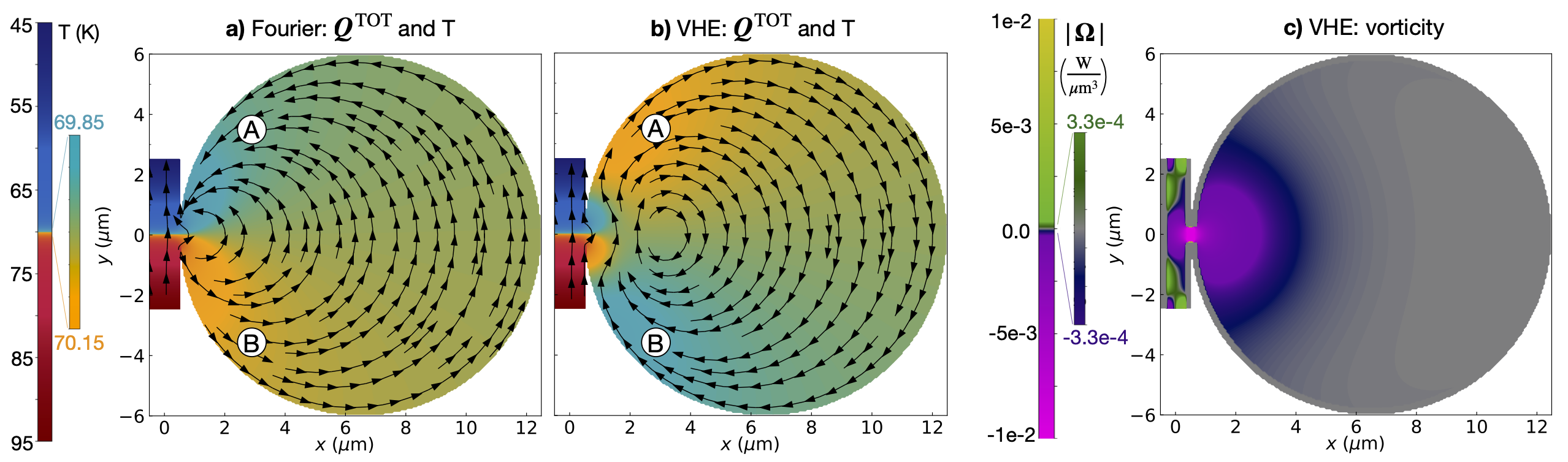
Figure 1: Signature of viscous heat backflow in graphite. In-plane ($x{-}y$) heat flux (streamlines) and temperature profile (colormap) for a tunnel-chamber device made of graphite. Panel a (b) shows the solution of Fourier’s equation (VHE) in the presence of a temperature gradient applied at the tunnel’s boundaries ($70{\pm}25$ K at $y{=}{\pm}2.5\mu m$), and considering the other boundaries as adiabatic (i.e. $\nabla T{\cdot}\bm{\hat{n}}{=}0$, where $\bm{\hat{n}}$ is the versor orthogonal to the boundary) and, in the VHE, "slipping" ($\bm{u}{\cdot}\bm{\hat{n}}{=}0$). In Fourier’s case (a), the direction of the temperature gradient in the chamber mirrors that in the tunnel ($T_{A}{<}T_{B}$). In contrast, the VHE (b) account for an additional viscous component for the heat flux—not directly related to the temperature gradient, see text—allowing the emergence of viscous backflow and temperature gradient in the chamber reversed compared to the tunnel ($T_{A}{>}T_{B}$). Panel c), vorticity of the VHE heat flux, $\nabla{\times}\bm{Q}^{\rm TOT}$; the vorticity for Fourier’s flux (not reported) is trivially zero.

$$C\frac{\partial T({\bm{r}},t)}{\partial t}+\sum_{i,j=1}^{3}\alpha^{ij}\frac{\partial u^{j}({\bm{r}},t)}{\partial r^{i}}-\sum_{i,j=1}^{3}\kappa^{ij}\frac{\partial^{2}T({\bm{r}},t)}{\partial r^{i}\partial r^{j}}=\dot{q}({\bm{r}},t),$$ (1)

$$A^{i}\frac{\partial u^{i}({\bm{r}},t)}{\partial t}+\sum_{j=1}^{3}\beta^{ij}\frac{\partial T({\bm{r}},t)}{\partial r^{j}}-\sum_{j,k,l=1}^{3}\mu^{ijkl}\frac{\partial^{2}u^{k}({\bm{r}},t)}{\partial r^{j}\partial r^{l}}=-\sum_{j=1}^{3}\gamma^{ij}u^{j}({\bm{r}},t).$$ (2)

In these equations, $T({\bm{r}},t)$ and $\bm{u}({\bm{r}},t)$ emerge from the conservation of energy and quasi-conservation of crystal momentum in microscopic phonon collisions in the hydrodynamic regime, respectively [9]. The terminology “quasi-conservation” is used because momentum-dissipating Umklapp collisions are always present in real materials at finite temperature—in practice the magnitude of hydrodynamic effects depends on the relative strength between normal and Umklapp collisions—and the presence of Umklapp collisions is taken into account by the dissipative term $-\gamma^{ij}u^{j}({\bm{r}},t)$. The term $\dot{q}({\bm{r}},t)$ accounts for the space- and time-dependent energy exchange with an external heat source. The thermal conductivity $\kappa^{ij}$ and viscosity $\mu^{ijkl}$ quantify the response of the crystal to a perturbation of temperature and drift-velocity, respectively [9]. The coupling coefficients $\alpha^{ij}$ and $\beta^{ij}$ originate from the relation between energy and crystal momentum for phonons. All these parameters are determined exactly from the LBTE (i.e. accounting for the actual phonon band structure and full collision matrix) and with first-principles accuracy, details are reported in the Supplementary Material (SM). Finally, we recall that in the VHE framework the total heat flux ($\bm{Q}^{TOT}$) is determined by temperature gradient and drift velocity [9], i.e., $\bm{Q}^{TOT}{=}\bm{Q}^{\delta}{+}\bm{Q}^{D}$ where ${Q}^{\delta,i}{=}{-}\sum_{j}\kappa^{ij}\nabla^{j}T$ and ${Q}^{D,i}{=}\sum_{j}\alpha^{ij}u^{j}$.

The VHE encompass Fourier’s law and temperature waves [1, 2] as special limiting cases. Specifically, it can be shown that in the limit of strong crystal-momentum dissipation and negligible viscous effects ($\mu_{\mathrm{max}}{\to}0$ and $[\gamma_{\mathrm{max}}]^{-1}{\to}0$, where $\mu_{\mathrm{max}}$ and $\gamma_{\mathrm{max}}$ are the maximum component of the viscosity and Umklapp dissipation tensors) the VHE yield Fourier’s diffusive behavior [9], which is trivially irrotational. In contrast, we show in Sec. I of the SM that in the time-dependent regime and inviscid limit ($\mu{=}0$) the VHE reduce to the DPLE [1, 2] for temperature waves. Both the known Fourier and DPLE special limiting cases are obtained when viscous effects are negligible, the former in the steady-state and the latter in the transient domain. In the following we use first-principles calculations to parametrize the VHE for natural and isotopically purified graphite, as well in h¹¹BN ; thus we explore how viscosity affects the emergence of non-diffusive, hydrodynamic behavior for heat both in the steady-state and transient regimes.

Steady-state viscous heat backflow.—In Fig. 1 we investigate how viscosity affects steady-state thermal transport by comparing the numerical solution of Fourier’s (inviscid) equation (panel a) with that of the viscous VHE (panel b). We consider a graphitic device having tunnel-chamber geometry, i.e. a form that promotes vortical hydrodynamic behavior [44]. We highlight that the VHE temperature profile in the chamber is reversed compared to the temperature profile in the tunnel, a behavior completely opposite to that predicted by Fourier’s law. Panel c shows that this temperature inversion—which in principle can be detected in thermal-imaging experiments [45, 46, 47, 11, 49]—occurs in the presence of viscous vortical flow, as a consequence of heat backflowing against the temperature gradient. Importantly, in SM II we show that heat vortices are not limited to graphite, predicting their appearance also in h¹¹BN around 60 K.

To see how the vortex and consequent heat backflow in Fig. 1 require the presence of a finite thermal viscosity to emerge, we start by noting that in general the behavior of the device is described by Eqs. (1,2) in the steady-state. Then, if we consider the inviscid limit ($\mu^{ijkl}{=}0\;\forall\;i,j,k,l$), Eq. (2) for an isotropic material such as graphite and h¹¹BN in the in-plane direction (hereafter tensor indexes will be omitted for tensors that are proportional to the identity in the in-plane directions, see SM. VIII) reduces to $\beta\nabla T({\bm{r}},t){=}{-}\gamma\bm{u}({\bm{r}},t)$. This equation can be inserted into Eq. (1) to readily show that this inviscid limit is governed by a Fourier-like irrotational equation, where the total heat flux is solely determined by the gradient of the temperature field and thus backflow and vorticity cannot emerge . In contrast, when a non-zero thermal viscosity tensor is considered in Eq. (2), the drift velocity is no longer proportional to the temperature gradient, and thus the total heat flux $\bm{Q}^{TOT}{=}\bm{Q}^{\delta}{+}\bm{Q}^{D}{=}{-}\kappa\nabla T{+}\alpha\bm{u}$ cannot be simplified to an irrotational expression depending only on the gradient of a scalar temperature field. This demonstrates that the presence of a non-zero viscosity is a necessary condition to have non-zero vorticity and observe steady-state viscous heat backflow. However, having non-zero thermal viscosity is necessary but not sufficient to observe heat backflow; in fact, one also needs a device’s geometry and boundary conditions that ensure the presence of non-zero second derivative of the drift velocity, i.e., of a total heat flux with non-zero vorticity. In this regard, the tunnel-chamber geometry promotes non-homogeneities in the drift-velocity field, and we show in SM III that having at least partially ‘slipping’ boundaries (i.e., corresponding to reflective phonon-boundary scattering [51, 18, 52], ) is also necessary to observe temperature inversion due to viscous heat backflow. We note that the simulations in Fig. 1 have been performed at conditions where the Fourier Deviation Number (FDN) [9] predicted steady-state hydrodynamic deviations from Fourier law to be largest in graphite (at natural isotopic concentration), i.e., in a device having size 10 $\mu$m and around 70 K. SM IV discusses how viscous backflow depends on device’s size, average temperature, and isotopic disorder in graphite.

Transient viscous heat backflow.—Recent experiments in graphite have observed heat backflowing against the temperature gradient only in the time-dependent domain, in the form of second sound [16, 15] or lattice cooling [14]. The pioneering theoretical analyses have been performed relying on the microscopic LBTE [54, 16, 15, 55, 14] without resolving effects induced by a macroscopic (experimentally observable) thermal viscosity, or relying on the inviscid mesoscopic DPLE [1, 2, 3, 4, 5, 6, 7, 8]. It is therefore natural to wonder how the viscous heat backflow emerging from the VHE behaves in the time domain, and more precisely if there is a relationship between temperature waves and transient viscous heat backflow.

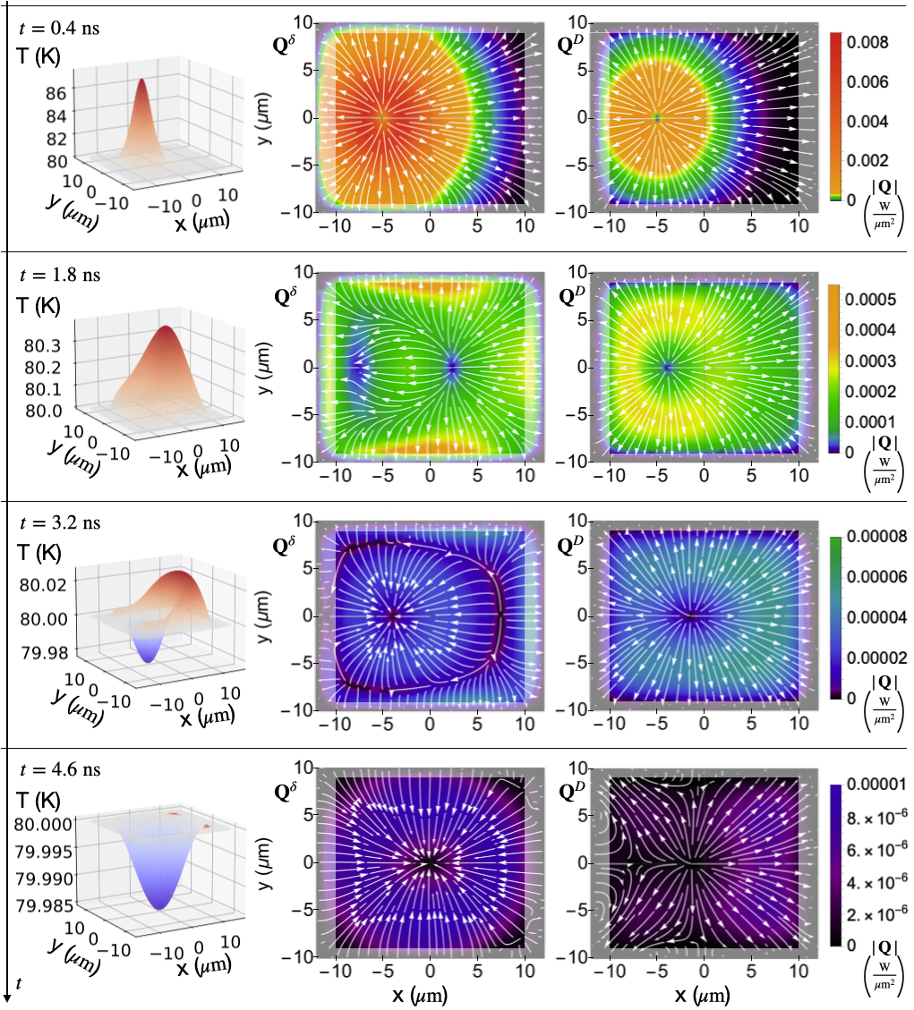
Figure 2: Transient hydrodynamic heat backflow and lattice cooling. We show the VHE predictions for the relaxation in time of a temperature perturbation (obtained applying a localized heater to the device for $0.0<t<0.4ns$) in a graphitic device thermalised at 80 K the boundaries (thermalisation occurs in shaded regions, see SM V). Rows show different instants in time for temperature (left column), temperature-gradient heat-flux component ($\bm{Q}^{\delta}$, central column), and drifting heat-flux component ($\bm{Q}^{D}$, right column). The emergence of transient heat backflow (temperature waves) originates from the lagged coupled evolution of $\bm{Q}^{\delta}$ and $\bm{Q}^{D}$, and is quantitatively affected by thermal viscosity, as discussed in the text. In the 2D plots, the heat-flux streamlines are shown in white, while the colormap shows the magnitude of the heat flux.

Therefore, we perform the time-dependent simulation shown in Fig. 2. We consider a rectangular device that is at equilibrium at $t{=}0\ \mathrm{ns}$ ($T{=}80$ K and $\bm{u}{=}0$ everywhere); we perturb it with a heater localized at $(x_{c},0)$ for $0{<}t{<}t_{\rm heat}{=}0.4\ \mathrm{ns}$ ($\dot{q}(\bm{r},t){=}\mathcal{H}\theta(t_{\rm heat}{-}t)\exp\left[{-}\tfrac{(x+x_{c})^{2}}{2\sigma_{x}^{2}}{-}\tfrac{y^{2}}{2\sigma_{y}^{2}}\right]$, see Eq. (1) and note [63]); at $t{=}t_{\rm heat}$ we switch off the heater and monitor the relaxation to equilibrium. The device is always thermalised at the boundaries ($T{=}80K$ and $\bm{u}{=}0$), see Ref. [11] for an experimental example of this boundary condition, and SM V for details on how boundary conditions (average temperature and thermalisation lengthscale), size, and isotopic-mass disorder affect the relaxation. The evolution of the temperature field (first column in Fig. 2) shows an oscillatory behavior, also termed “lattice cooling” [14] because of the transient and local appearance of temperature values lower than the initial equilibrium temperature. Such an oscillatory behavior is in sharp contrast with that predicted by Fourier’s diffusive equation (see SM VI), whose smoothing property [17] implies that the evolution of a smooth, positive temperature perturbation relaxes to equilibrium remaining non-negative with respect to the initial equilibrium values. The appearance of lattice cooling from the VHE can be understood by inspecting the time evolution of the two aforementioned components of the VHE’s heat flux ($\bm{Q}^{\delta}$ and $\bm{Q}^{D}$). The heat-flow streamlines in the second and third column of Fig. 2 show that the heat fluxes $\bm{Q}^{\delta}$ and $\bm{Q}^{D}$ can assume opposite directions during the relaxation, with the drifting flux $\bm{Q}^{D}{\propto}\bm{u}$ backflowing against the temperature-gradient flux $\bm{Q}^{\delta}{\propto}{-}\nabla T$. This is a consequence of the lagged (delayed) coupling between $\bm{Q}^{\delta}$ and $\bm{Q}^{D}$ in the VHE (1,2), which in the inviscid limit ($\mu{=}0$) reduces exactly to the lagged relationship between heat flux and temperature gradient discussed in the context of the dual-phase-lag model [2]. Specifically, we show in SM I that in the inviscid limit $\bm{Q}^{TOT}(\bm{r},t{+}\tau_{Q}){=}{-}\kappa\nabla T(\bm{r},t{+}\tau_{T})$, where $\tau_{Q}{=}A/\gamma$ is the delay between the application of a temperature gradient and the appearance of a heat flux, and $\tau_{T}{=}\kappa A/(\alpha\beta{+}\kappa\gamma)$ is the time needed to create temperature gradient from an established heat flux (here tensor/vector indexes are omitted because in-plane transport in graphite is isotropic [3, 9]). Thus, heat backflow can be observed in the time-dependent domain as a consequence of different characteristic timescales for the evolution of $\bm{Q}^{\delta}$ and $\bm{Q}^{D}$, which allow these two heat-flux components to flow in opposite directions and yield in the inviscid limit a behavior analytically equivalent to the lagged DPLE. This also shows that while steady-state hydrodynamic heat backflow can emerge exclusively as a consequence of a finite thermal viscosity, time-dependent hydrodynamic backflow (i.e., temperature oscillations) do not necessarily require viscosity to appear (see SM VI for details). Nevertheless, we show in the following and in SM VII that accounting for a finite thermal viscosity is necessary to obtain quantitative agreement between the hydrodynamic relaxation lengthscales and timescales predicted from theory and observed in experiments.

Resonant amplification of temperature waves.—The temperature waves observed in Fig. 2 have a small amplitude and consequently are difficult to be detected in experiments. Nevertheless, they are expected to exhibit resonant amplification when driven with a perturbation periodic in time, and this could be exploited to facilitate their experimental detection. Therefore, we investigate quantitatively the behavior of the device in Fig. 2 when driven with a periodic perturbation. Considering the analogies between temperature and mechanical waves, we applied to the device in Fig. 2 a perturbation mathematically similar to the $(1,2)$ mode of a loaded rectangular membrane, i.e. $\dot{q}(\bm{r},t){=}\mathcal{H}[\sin(\omega t){+}1]\exp\big{[}{-}\tfrac{(x{+}x_{c})^{2}}{2\sigma_{x}^{2}}{-}\tfrac{y^{2}}{2\sigma_{y}^{2}}\big{]}{+}$ ${+}\mathcal{H}[\sin(\omega t{+}\pi){+}1]\exp\big{[}{-}\tfrac{(x-x_{c})^{2}}{2\sigma_{x}^{2}}{-}\tfrac{y^{2}}{2\sigma_{y}^{2}}\big{]}$. This perturbation is always non-negative, representing the laser heating employed in experiments [16, 14, 15]. Then, we monitored how the amplitude of the temperature oscillation, $a$, varies as a function of frequency, $f$. Fig. 3 shows that the solution of the periodically driven VHE in natural graphite displays resonant behavior, i.e. plotting the oscillation amplitude as a function of frequency, $a(f)$, we see a peak reminiscent of that observed in the frequency response of a driven underdamped oscillator. We highlight how the resonant behavior obtained from the viscous VHE is weaker than that obtained from the inviscid DPLE, while Fourier’s law completely lacks resonant response (analogously to an overdamped mechanical oscillator). We also note that the analysis in Fig. 3 improves upon previous studies based on the inviscid DPLE [10, 3, 7] by providing insights into how the resonant behavior of temperature waves is affected by thermal viscosity. Finally, the inset shows that reducing isotopic-mass disorder in graphite yields a stronger VHE resonant response, and that analogous signatures are expected to emerge in h¹¹BN around $T{=}60K$ and in slightly smaller (15$\mu m$-long) devices.

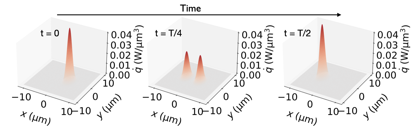
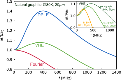
Figure 3: Resonant amplification of temperature waves. Top, two-spots periodic perturbation ($\dot{q}(\bm{r},t)$ in Eq. 1) applied to rectangular device made of graphite and having dimension and boundary conditions as in Fig. 2. Bottom, resonant amplification, of temperature oscillations around $T{=}80K$ predicted by the VHE (green) and DPLE (blue). Red is Fourier’s law, lacking amplification. The main plot refers to graphite at natural-abundance isotopic-mass disorder (98.9% ${}^{12}C$, 1.1% ${}^{13}C$). Inset, the VHE predict that isotopically pure samples of graphite (99.9% ${}^{12}C$, 0.1% ${}^{13}C$, dashed dark green) feature a stronger resonant amplification compared to natural graphite (green, same as in the main plot); in addition, analogous signatures are predicted to appear in h¹¹BN, around $T{=}60K$ and in slightly smaller (15$\mu m$-long) devices.

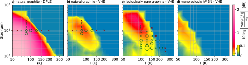
Figure 4: Maximum resonant amplification as a function of size, temperature, and isotopic disorder. The colormaps show the maximum resonant amplification (see text) as a function of the characteristic size of the rectangle [66] and of the average temperature around which the perturbation is applied. Panels a,b) refer to natural graphite, a) is the DPLE and b) the VHE. Empty green circles have an area proportional to the hydrodynamic strength [67] measured in experiments by Huberman et al. [16] for natural samples, and by Ding et al. [15] for isotopically pure samples; the red crosses correspond to conditions under which experiments observed diffusive behavior (lack of hydrodynamics). We highlight how the VHE (b) capture the temperatures and lengthscales at which hydrodynamic behavior was observed; in contrast, the inviscid DPLE misses the disappearance of hydrodynamic behavior at low temperature. Panel c), VHE hydrodynamic behavior in isotopically pure graphite, in broad agreement with experiments from Ref. [15]. Panel d), VHE resonant behavior predicted in h¹¹BN.

Next, we systematically investigate how the maximum resonant amplification vary as a function of device size, average temperature, and type of material. We performed simulations analogous to Fig. 3 varying device’s size and equilibrium temperature, computing for every simulation the maximum resonant amplification as ${\rm max}_{f}[a(f)]/a_{0}$ (where $a_{0}{=}\lim_{f{\to}0}a(f)$, see Fig. 3). In Fig 4a,b we compare the inviscid DPLE (a) with the VHE (b) in natural graphite. We see that the temperatures and lengthscales at which the VHE predict the emergence of hydrodynamic resonant behavior in natural samples are in broad agreement with the temperatures and lengthscales for the emergence of heat hydrodynamics discussed by Huberman et al. [16]; in contrast, the DPLE fails to capture the reduction of hydrodynamic behavior as temperature is decreased below 100 K. Turning our attention to isotopically pure graphite (Fig. 4c), we see that here the VHE resonant response is stronger than in natural graphite, and it also persists up to larger lengthscales and higher temperatures, in broad agreement with the experiments by Ding et al. [15]. Finally, Fig. 4d predicts that resonant behavior for viscous temperature waves occurs also in h¹¹BN, with a magnitude slightly weaker than in natural graphite.

Conclusion.—We have shed light on the fundamental physics determining the emergence of viscous heat hydrodynamics, discussing with quantitative first-principles accuracy how to induce temperature inversion in steady-state heat vortices, and viscous temperature waves in extreme thermal conductors such as graphite and layered h¹¹BN. We have demonstrated that these phenomena can be amplified by engineering the device’s boundary conditions or exploiting resonance, paving the way for applications in next-generation electronic and phononic technologies. We have provided novel, fundamental insights on temperature waves, showing that the viscous temperature waves emerging from the VHE differ fundamentally from the inviscid DPLE heat waves [1, 2, 10, 3, 7]. Most importantly, we have quantitatively demonstrated that viscous effects determine the hydrodynamic relaxation timescales [14] and lengthscales [16, 15] measured in pioneering experiments. These results share fundamental common underpinnings with other quasiparticle’s fluid-like transport phenomena in solids—involving, e.g., electron-phonon bifluids [44, 70, 71, 72, 73, 74, 75, 76], magnons [77], skyrmions [78]—thus will potentially inspire analogous developments and applications. Finally, our findings may also directly translate to fluids flowing in porous media, and are thus relevant for soil science, groundwater hydrology, and petroleum engineering [79].

We thank Dr Miguel Beneitez, Dr Gareth Conduit, and Dr Orazio Scarlatella for the useful discussions. M. S. acknowledges support from Gonville and Caius College, and from the SNSF project P500PT_203178. J. D. thanks Prof Hrvoje Jasak for his hospitality in Cambridge. The first-principles calculations of conductivity and viscosity were performed on the Sulis Tier 2 HPC platform, funded by EPSRC Grant EP/T022108/1 and the HPC Midlands+consortium.

Supplementary material

I DPLE as inviscid limit of the VHE

In this section we show analytically that the dual-phase-lag equation (DPLE) [1, 2], widely used to describe temperature waves [3, 4, 5, 6, 7, 8], emerges from the viscous heat equations (VHE) [9] in the limit of vanishing viscosity. To see this, we start from the VHE without the viscosity and source term,

$$C\frac{\partial T(\bm{r},t)}{\partial t}{+}\!\!\sum_{ij}\alpha^{ij}\frac{\partial u^{j}(\bm{r},t)}{\partial x^{i}}{-}\!\!\sum_{ij}\kappa^{ij}\frac{\partial^{2}}{\partial x^{i}\partial x^{j}}T(\bm{r},t){=}0,\hskip 17.07164pt$$ (S1)

$$A_{k}\frac{\partial u_{k}(\bm{r},t)}{\partial t}+\sum_{i}\gamma^{i}_{k}u^{i}(\bm{r},t)+\sum_{i}\beta^{i}_{k}\frac{\partial T(\bm{r},t)}{\partial x^{i}}=0,\hskip 28.45274pt$$ (S2)

where the indexes $i,k$ denote Cartesian directions. Then we consider a setup where the tensors appearing in Eqs. (S1,S2) can be considered diagonal and isotropic (as is the case for a device mode of graphite or h¹¹BN with non-homogeneities exclusively in the basal plane, see Sec. VIII). Thus, writing the second equation by components for the $2$-dimensional case we have:

$$C\frac{\partial T}{\partial t}+\alpha\left(\frac{\partial u_{x}}{\partial x}+\frac{\partial u_{y}}{\partial y}\right)-\kappa\left(\frac{\partial^{2}T}{\partial x^{2}}+\frac{\partial^{2}T}{\partial y^{2}}\right)=0,\hskip 22.76219pt$$ (S3)

$$A\frac{\partial u_{x}}{\partial t}+\gamma u_{x}+\beta\frac{\partial T}{\partial x}=0,\hskip 56.9055pt$$ (S4)

$$A\frac{\partial u_{y}}{\partial t}+\gamma u_{y}+\beta\frac{\partial T}{\partial y}=0.\hskip 56.9055pt$$ (S5)

Deriving both sides of Eq. (S4) with respect to $x$, and both sides of Eq. (S5) with respect to $y$, we obtain:

$$\left(A\frac{\partial}{\partial t}+\gamma\right)\frac{\partial u_{x}}{\partial x}=-\beta\frac{\partial^{2}T}{\partial x^{2}};$$ (S6)

$$\left(A\frac{\partial}{\partial t}+\gamma\right)\frac{\partial u_{y}}{\partial y}=-\beta\frac{\partial^{2}T}{\partial y^{2}}.$$ (S7)

Then, we sum Eq. (S6) and Eq. (S7), obtaining:

$$\left(A\frac{\partial}{\partial t}{+}\gamma\right)\!\!\left(\frac{\partial u_{x}}{\partial x}{+}\frac{\partial u_{y}}{\partial y}\right)\!{=}{-}\beta\bigg{(}\frac{\partial^{2}T}{\partial x^{2}}{+}\frac{\partial^{2}T}{\partial y^{2}}\bigg{)}.\hskip 14.22636pt$$ (S8)

Now we notice that applying the operator $\hat{\mathcal{O}}=\left(A\frac{\partial}{\partial t}{+}\gamma\right)$ to both sides of Eq. (S3), and by using Eq. (S8), allows us to write an equation for temperature only:

$$\begin{gathered}\frac{CA}{\gamma}\frac{\partial^{2}T}{\partial t^{2}}+C\frac{\partial T}{\partial t}-\left(\frac{\alpha\beta}{\gamma}+\kappa\right)\left(\frac{\partial^{2}T}{\partial x^{2}}+\frac{\partial^{2}T}{\partial y^{2}}\right)\\ -\frac{\kappa A}{\gamma}\frac{\partial}{\partial t}\left(\frac{\partial^{2}T}{\partial x^{2}}+\frac{\partial^{2}T}{\partial y^{2}}\right)=0.\end{gathered}$$ (S9)

Eq. (S9) is exactly the DPLE equation discussed by Joseph and Preziosi [1] and Tzou [2]. We can now see the relationship between the constants appearing in the VHE, and the time lags appearing in the DPLE [2] and discussed in the main text: $\tau_{T}=\frac{\kappa A}{\alpha\beta+\kappa\gamma}$, $\tau_{Q}=\frac{A}{\gamma}$. We conclude by noting that the thermal diffusivity appearing in the DPLE is $\alpha_{E}=\frac{\alpha\beta+\kappa\gamma}{C\gamma}$. It can be readily seen that in the limit $\tau_{T}=\tau_{Q}$, as well as in the steady-state, the DPLE becomes equivalent to Fourier’s law, while in the limit $\tau_{T}=0$ it becomes equivalent to Cattaneo’s second-sound equation [2].

In summary, the above derivation demonstrates that the viscous temperature waves emerging from the VHE are fundamentally different from the inviscid DPLE heat waves previously discussed in the literature [1, 2, 10, 3, 7].

II Steady-state viscous heat backflow in ${\rm h}^{11}$BN

In this section we show that the emergence of heat vortices is not limited to graphite, predicting their appearance also in a device made of h¹¹BN (Fig. S1).

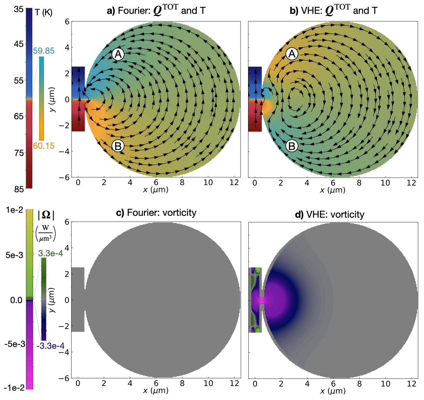
Figure S1: Signature of viscous heat backflow in h¹¹BN. In-plane ($x{-}y$) heat flux (streamlines) and temperature profile (colormap) for a tunnel-chamber device made of h¹¹BN. Panel a (b) shows the solution of Fourier’s equation (VHE) in the presence of a temperature gradient applied at the tunnel’s boundaries ($60{\pm}25$ K at $y{=}{\pm}2.5\mu m$), and considering the other boundaries as adiabatic (i.e. $\nabla T{\cdot}\bm{\hat{n}}{=}0$, where $\bm{\hat{n}}$ is the versor orthogonal to the boundary) and, in the VHE, "slipping" ($\bm{u}{\cdot}\bm{\hat{n}}{=}0$). In Fourier’s case (a), the direction of the temperature gradient in the chamber mirrors that in the tunnel ($T_{A}{<}T_{B}$). In contrast, the VHE (b) account for an additional viscous component for the heat flux—not directly related to the temperature gradient, see main text—allowing the emergence of viscous backflow and temperature gradient in the chamber reversed compared to the tunnel ($T_{A}{>}T_{B}$). Panel c), the vorticity Fourier’s heat flux is trivially zero; panel d) shows the non-zero vorticity of the total VHE heat flux, $\nabla{\times}\bm{Q}^{\rm TOT}$.

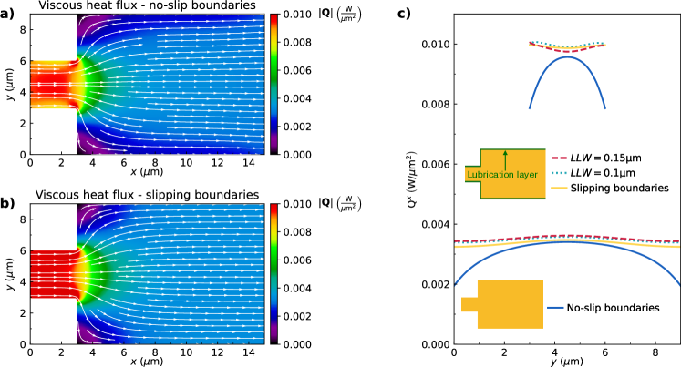
Figure S2: Effects of boundary conditions on the heat-flux profile. In-plane (x-y) heat fluxes in graphite, obtained solving the VHE imposing a temperature of $80\ \mathrm{K}$ on the left side ($x=0\ \mathrm{\mu m}$) and $60\ \mathrm{K}$ on the right side ($x=15\ \mathrm{\mu m}$), assuming all boundaries at $x\neq 0\ \mathrm{\mu m}$ and $x\neq 15\ \mathrm{\mu m}$ to be adiabatic, and using no-slip boundary conditions for the drift velocity ($\bm{u}{=}\bm{0}$ at the boundary) in a) [9], and a perfectly slipping boundary condition ($\bm{u}\cdot\bm{\hat{n}}=0$, where $\bm{\hat{n}}$ is the versor orthogonal to the boundary) in panel b). Panel c), differences between the heat-flow profile along the vertical sections $x=1.5\ \mathrm{\mu m}$ and $x=9\ \mathrm{\mu m}$ for different boundary conditions. We highlight how the lubrication-layer approach, used to model slipping boundaries in a numerically convenient way, allows to obtain results practically indistinguishable from those obtained exactly implementing the slipping boundaries. The insets in panel c) show schematically how the lubrication layer is implemented.

III Boundary conditions used in steady-state simulations

III.1 Lubrication layer and slipping boundaries

In this section we discuss the numerical techniques used to simulate different boundary conditions for the drift velocity. Specifically, in order to model boundary conditions different from no-slip ($\bm{u}{=}\bm{0}$ at the boundary), which correspond to boundaries that are completely dissipating the crystal momentum, we introduce a "lubrication layer", i.e. a region in proximity of the actual boundary in which the viscosity is greatly reduced ($\mu^{ijkl}_{\rm lub}=\mu^{ijkl}/F$, where $F{\geq}1$). By imposing a no-slip condition on the actual boundary of the device, choosing a lubrication layer width (LLW) to be small ($\lesssim 5\%$ of the device’s characteristic size), and varying the factor $F$ from 1 to an arbitrarily large number, one can mimic the effect of boundary conditions ranging from no-slip ($\bm{u}{=}\bm{0}$, $F{=}1$) to perfectly slipping ($F{\to}\infty$). In fact, by reducing the viscosity in the lubrication layer, one reduces the viscous stresses due to presence of the boundary, with the limit $F{=}1$ representing no reduction and yielding the no-slip condition, and the limit $F{\to}\infty$ representing infinite reduction, i.e. perfectly slipping boundaries.

We show in Fig. S2 that, in analogy to standard fluid-dynamics, no-slip boundary conditions (panel a, also discussed in Ref. [9]) yield a Poiseuille-like heat-flow profile. In contrast, using slipping boundaries yield much weaker (negligible) variations of the heat-flux profile (panel b). The lubrication-layer approach is particularly advantageous from a numerical viewpoint. In fact, in standard solvers such as Wolfram Mathematica, implementing perfectly slipping boundary conditions is straightforward in simple geometries such as that in Fig. S2, where the Cartesian components of the drift velocity are always aligned or orthogonal to the boundaries. However, in complex geometries such as that in Fig. 1, it is not possible to find a coordinate system which is always aligned or orthogonal to the boundaries, rendering the numerical implementation of the slipping boundary conditions much more complex. We show in Fig. S2c) that by choosing a sufficiently small LLW, and a sufficiently large value for the viscosity reduction factor ($F=10^{4}$), one obtains practically indistinguishable results by using the lubrication layer or the exact slipping boundary conditions.

Thus, the test reported in Fig. S2 justifies the usage of the lubrication layer to simulate slipping boundary conditions in a numerically affordable way. Such an approach has been used to model the complex geometry shown in Fig. 1, in particular we chose a LLW=0.1 $\mu m$ and a viscosity reduction factor $F=1000$ for the lubrication layer. We conclude by noting that in Fig. S2 a) and b) the area where viscosity assumes the physical value has exactly the same size.

III.2 Slipping boundaries and heat vortices

After having shown in Sec. III.1 that the lubrication layer allows to model boundary conditions for the drift velocity ranging from no-slip to perfectly slipping, we use this approach to study how the inversion of the temperature gradient observed in Fig. 1 depends on the boundary conditions. Fig. S3 shows how the lubrication layer and external baths at fixed temperature are applied to the tunnel-chamber geometry of Fig. 1.

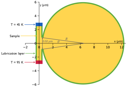
Figure S3: Channel-chamber geometry for observation of steady-state viscous heat backflow. The yellow region is the simulation domain where all the parameters entering in the VHE assume physical values; the green area is the lubrication-layer region, where the viscosity is reduced by a factor $F$ to account for partially reflective boundaries. The width of the lubrication layer (0.1 $\mu m$), and of the opening connecting the tunnel and the chamber (0.52 $\mu m$), are represented in an exaggerated way for graphical clarity. The opening angle used here and in Fig. 1 is $\theta=4.9672^{\circ}$. A temperature of 95 K (45 K) is applied at the lower (upper) opening of the tunnel, all the other boundaries are adiabatic.

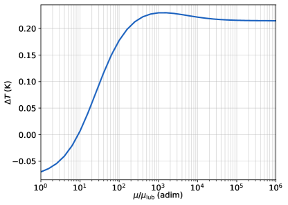
Figure S4: Dependence of the temperature inversion due to viscous backflow on the boundary conditions. We plot the temperature difference $\Delta T=T_{\mathrm{A}}-T_{\mathrm{B}}$, where $A=(3,3.5)\mu m$ and $B=(3,-3.5)\mu m$, measured in the circular chamber of Fig. 1 as a function of the reduction of viscosity in the lubrication layer with LLW=$0.1\mu m$. As the viscosity in the lubrication layer is reduced, the drifting component of the heat flow encounters less resistance when flowing tangential to the circular boundary. This analysis was performed simulating samples with isotopic-mass disorder at natural concentration.

The large temperature gradient applied at the extremities of the tunnel creates a drift velocity, thanks to the coupling between temperature gradient and drift-velocity shown in Eq. (2). Therefore, significant values for both the temperature-gradient ($\bm{Q}^{\delta}$) and drift-velocity ($\bm{Q}^{D}$) heat fluxes are present at the opening of the circular chamber. When these heat fluxes leak into the chamber they are subject to a significant gradient; for the drift-velocity component of the heat flux, a significant gradient causes viscous shear, and the vortex forms to minimize such shear. In contrast, as discussed in the main text, viscous forces are absent in Fourier’s law, which trivially yields an irrotational flow.

Now we want to investigate how the signature of viscous heat backflow discussed in Fig. 1, i.e. the temperature gradient in the chamber reversed compared to the tunnel, depends on the boundary conditions. To this aim, we look at how the temperature difference between two points in the chamber $A=(3,3.5)\mu m$ and $B=(3,-3.5)\mu m$ depends on the boundary conditions adopted. Positive temperature difference $\Delta T=T_{A}-T_{B}$ is observed when viscous heat backflow causes a behavior analogous to Fig. 1b, while negative temperature difference is obtained when the system displays a behavior analogous to Fourier’s law (Fig. 1a). We show in Fig. S4 how such temperature difference changes as a function of the viscosity reduction in the lubrication layer. We see that as the viscosity in the lubrication layer is reduced, $\Delta T$ switches from negative (Fourier-like) to positive (vortex-like), indicating that (at least partially) slipping boundaries are needed to observe the temperature inversion related to viscous heat backflow. We highlight how, in the limit of vanishingly low viscosity for the lubrication layer, the temperature inversion $\Delta T$ converges to a constant, indicating that the viscosity in the lubrication layer is so reduced that the overall effect is that of perfectly slipping boundaries.

In summary, the results in Fig. S4 suggest that smooth boundaries are needed to observe heat vortices and related temperature inversion, and conversely measurements of hydrodynamic heat transport may be used to characterize the roughness of devices’ boundaries, i.e. their capability to reflect phonon’s crystal momentum.

IV Effects of temperature, size, and isotopes on viscous heat backflow

In this section we explore how the temperature inversion due to viscous heat backflow depends on the size of the device, the average temperature around which the temperature gradient is applied, and the presence of isotopic-mass disorder in graphite (this latter affects the parameters such as intrinsic thermal conductivity and intrinsic thermal viscosity of the sample). We show in S5 that the temperature inversion due to viscous heat backflow is maximized at average temperatures below 100 K for natural graphite (98.9 % ¹²C, 1.1 % ¹³C) and below 110 K for isotopically purified graphite (99.9 % ¹²C, 0.1 % ¹³C).

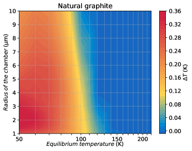
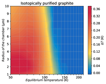
Figure S5: Effects of temperature, size, and isotopic disorder on viscous heat backflow. The colormap shows how the temperature inversion due to viscous backflow, computed as the difference between the maximum temperature in the upper part of the chamber ($y>0\mu m$) and the minimum temperature in the lower part in the chamber ($y<0\mu m$), depends on the radius of the chamber and on the average temperature ${T}_{\rm eq}$ of the tunnel (a perturbation of $\delta T={T}_{\rm eq}\pm 25K$ is always used at the extremities of the tunnel). The upper panel refers to samples with natural-abundance isotopic disorder, the lower panel shows isotopically pure samples.

Moreover, the temperature inversion is not significantly affected by the chamber’s radius, and it is slightly larger in isotopically pure samples compared to natural samples. We note finite-size effects on the parameters entering in the VHE have been taken into account following the approach detailed in Ref. [9] and considering a grain size equal to the diameter of the chamber.

V Boundary conditions for time-dependent simulations

V.1 Thermalisation lengthscale

In actual experimental devices thermalisation is not perfectly localized in space, but occurs over a finite lengthscale [11], i.e. there is a smooth transition from the device interior to the thermal bath. Therefore, we model the boundaries relying on a compact sigmoid function [12] to smoothly connect the a thermal bath region, where temperature is fixed and drift velocity is zero (since at equilibrium phonons are distributed according to the Bose-Einstein distribution, which has zero drift velocity [9]), and the device’s interior, where the evolution of temperature and drift velocity is governed by the viscous heat equations. Specifically, we used the smooth-step function [13] that is ubiquitously employed in numerical calculations, i.e. a sigmoid Hermite interpolation between $0$ and $1$ of a polynomial of order $5$:

$$f(r){=}\begin{cases}0,&{\rm if\;}\hskip 14.22636ptd(r)<0\\ 1,&{\rm if\;}\hskip 14.22636ptd(r)>1\\ {6[d(r)]^{5}{-}15[d(r)]^{4}{+}10[d(r)]^{3},}&{\rm otherwise}\end{cases}$$ (S10)

where $d(r)=\left(\frac{r{-}R_{in}}{R_{out}{-}R_{in}}\right)$ and $r>0$, as well as $R_{\text{in}}>0$ and $R_{\text{out}}>0$. The function is second order continuous and saturates exactly to zero and one at the points $R_{\text{in}}$ and $R_{\text{out}}$, respectively. We show in Fig. S6 the sigmoid function (S10) for $R_{\text{in}}=10\mu m$ and $R_{\text{out}}$ ranging from 11 to 20 $\mu m$: $R_{\text{out}}{\simeq}R_{\text{in}}$ simulates an ideal thermalisation (occurring over a negligible lengthscale), while $R_{\text{out}}{\gg}R_{\text{in}}$ simulates a very inefficient (non-ideal) thermalisation that occurs over a very large lengthscale. Then, relying on the sigmoid (S10) we connected smoothly the thermal bath region, where $f(\bm{r})=1$, $T({\bm{r}},t)={T}_{\rm eq}$, and $\bm{u}({\bm{r}},t)=\bm{0}$, with the device’s interior region, where $f(\bm{r})=0$ and the evolution of $T({\bm{r}},t)$ and $\bm{u}({\bm{r}},t)$ is governed by the VHE.

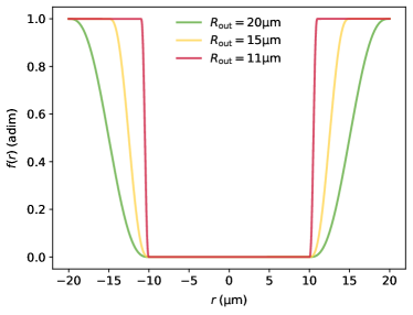
Figure S6: Sigmoid function to model realistic thermalisation. The sigmoid function (S10) is plotted for $R_{\text{in}}=10\mu m$ and various values of $R_{\text{out}}$. $R_{\text{out}}=11\mu m$ (red) simulates a thermalisation that occurs over a very short lengthscale and is thus close to ideal, $R_{\text{out}}=15\mu m$ (orange) is an estimate of a realistic thermalisation length [11], and $R_{\text{out}}=20\mu m$ (green) represents thermalisation less efficient than in the previous cases.

In formulas, we have that

$$f(\bm{r})[T({\bm{r}},t)-{T}_{\rm eq}]+[1-f(\bm{r})]\left(C\frac{\partial T({\bm{r}},t)}{\partial t}+\sum_{i,j=1}^{3}\alpha^{ij}\frac{\partial u^{j}({\bm{r}},t)}{\partial r^{i}}-\sum_{i,j=1}^{3}\kappa^{ij}\frac{\partial^{2}T({\bm{r}},t)}{\partial r^{i}\partial r^{j}}-\dot{q}({\bm{r}},t)\right)=0,$$ (S11)

$$f(\bm{r})u^{i}({\bm{r}},t)+[1-f(\bm{r})]\left(A^{i}\frac{\partial u^{i}({\bm{r}},t)}{\partial t}+\sum_{j=1}^{3}\beta^{ij}\frac{\partial T({\bm{r}},t)}{\partial r^{j}}-\sum_{j,k,l=1}^{3}\mu^{ijkl}\frac{\partial^{2}u^{k}({\bm{r}},t)}{\partial r^{j}\partial r^{l}}+\sum_{j=1}^{3}\gamma^{ij}u^{j}({\bm{r}},t)\right)=0.$$ (S12)

Details on how the non-ideal thermalisation affects the magnitude of signatures of heat hydrodynamics are reported later in this document.

V.2 Modeling realistic thermalisation in a rectangular geometry

In order to apply the realistic-thermalisation boundary conditions discussed in Sec. V.1 to the rectangular device of Fig. 2, we employed a smoothed rectangular domain, since we noted that smooth simulation domains yielded better computational performances (faster convergence with respect to the discretization mesh, reduced numerical noise) compared to non-smoothed rectangular domains. The equation defining the smoothed rectangular domain employed in Figs. 2,3,4 is:

$$\left(\frac{|x|}{a_{\rm out}}\right)^{\frac{2a_{\rm out}}{\lambda}}+\left(\frac{|y|}{b_{\rm out}}\right)^{\frac{2b_{\rm out}}{\lambda}}=1,$$

where $a_{\rm out}$ and $b_{\rm out}$ are the sides of the rectangular domain where the thermalisation is perfect (outside the dashed-lime region in Fig. S7); $\lambda$ controls the smoothness of the corners, and we used $\lambda=\frac{a_{\rm out}}{3}$ to obtain a domain smooth enough for numerical purposes and sharp enough to practically model a rectangular device. We note that the sigmoid function (S10) has to be adapted be employed in a rectangular geometry. Specifically, in Eq. (S10) in place of the distance $r$ we used a distance of the form

$$\tilde{r}(x,y)=\left[\left(\frac{|x|}{a_{\rm out}}\right)^{\frac{2a_{\rm out}}{\lambda}}+\left(\frac{|y|}{b_{\rm out}}\right)^{\frac{2b_{\rm out}}{\lambda}}\right]^{1/p},$$ (S13)

where $p$ controls the nonlinearity in which the two terms in Eq. (S13) are combined, and we chose $p=20$ (this value will be justified later).

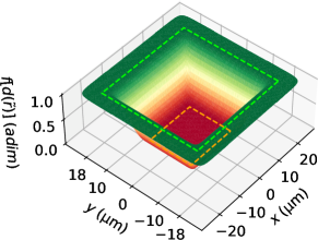
Figure S7: Sigmoid function to model realistic thermalisation in rectangular geometry. Green (outside the dahsed-lime line) is the perfectly thermalised region, where the sigmoid function $f\big{(}d(\tilde{r})\big{)}=1$, and the thermal reservoir ensures that temperature is perfectly constant and the drift velocity is zero. Red (inside the dashed-orange line) represents the inner "free" region where $f\big{[}d(\tilde{r})\big{]}=0$ and the evolution of temperature and drift velocity is determined by the VHE.

Then, the distance (S13) is nested into the function $d(\tilde{r})=\left(\frac{\tilde{r}(x,y){-}R_{in}}{R_{out}{-}R_{in}}\right)$. It is evident that $d(\tilde{r})<0$ when $\tilde{r}(x,y){<}R_{\rm in}$, and $d(\tilde{r})>1$ when $\tilde{r}(x,y){>}R_{\rm out}$. Therefore, if one sets $R_{\text{in}}=\tilde{r}(a_{\text{in}},b_{\text{in}})$, and $R_{\text{out}}=\tilde{r}(a_{\text{out}},b_{\text{out}})$, and inserts $d(\tilde{r})$ into Eq. (S10), the resulting function $f[d(\tilde{r})]$ is exactly zero inside the rectangle having sides $a_{\text{in}},b_{\text{in}}$ (red region in Fig. S7, where the evolution of temperature and drift velocity is determined by the VHE) and exactly one outside the rectangle having side $a_{\text{out}},b_{\text{out}}$ (green region in Fig. S7, where the thermal reservoir ensures that temperature is perfectly constant and the drift velocity is zero). The value of $p$ in Eq. (S13) affects how the sigmoid function goes from zero to one between the dashed-orange and dashed-green rectangles, and the aforementioned value $p=20$ was chosen after checking that the overall transition was sufficiently smooth for numerical purposes (Fig. S7). In the next section we investigate how the thermalisation lengthscale, $a_{\rm out}{-}a_{\rm in}$, affects lattice cooling (this investigation will be done varying only $a_{\rm out}$, $b_{\rm out}$ in the above equations and keeping all the other parameters fixed).

V.3 Dependence of VHE lattice cooling on the boundary conditions

In this section we investigate how the magnitude of the viscous temperature oscillations discussed in Fig. 2 depends on the thermalisation lengthscale at the boundaries. In order to quantify the magnitude of temperature oscillations, we define a descriptor to capture the “lattice cooling stregth” (LCS)

$$LCS=\frac{T_{\mathrm{eq}}-T_{\mathrm{min}}}{T_{\mathrm{max}}-T_{\mathrm{min}}},$$ (S14)

where $T_{\mathrm{max}}=\max_{t}[T(\bm{r}_{c},t)]$ and $T_{\mathrm{min}}=\min_{t}[T(\bm{r}_{c},t)]$ are the maximum and minimum temperatures, respectively, observed during the relaxation in the point $\bm{r}_{c}{=}(x_{c},0)$, where the perturbation

$$\dot{q}(\bm{r},t){=}\mathcal{H}\;\theta(t_{\rm heat}{-}t)\exp\left[-\tfrac{(x+x_{c})^{2}}{2\sigma_{x}^{2}}{-}\tfrac{y^{2}}{2\sigma_{y}^{2}}\right]$$ (S15)

is centered. We recall that we used $\mathcal{H}=0.013\tfrac{W}{\mu m^{3}}$, $t_{\rm heat}=0.4ns$, $x_{c}=5\mu m$, $\sigma_{x}=2\mu m$, $\sigma_{y}=2.8\mu m$, to ensure that the perturbation created causes variations within 10% of the equilibrium temperature ($T_{eq}=80K$).

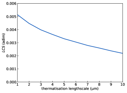
Figure S8: Dependence of lattice cooling strength on the thermalisation lengthscale. We show how LCS in a device having non-thermalised region equal to $20\ \mathrm{\mu m}{\times}16\ \mathrm{\mu m}$ (as in Fig. 2) depends on the thermalisation lengthscale, i.e. the length over which the sigmoid function shown in Fig. S6 goes from zero to one. Even if LCS decreases as the thermalisation lengthscale increases, LCS remains appreciable even at thermalisation lengthscales as large as 10 $\mu m$.

Clearly, LCS is zero if lattice cooling does not take place, and assumes a positive value if lattice cooling occurs. To gain insights on how lattice cooling is affected by the thermalisation lengthscale, we fixed the size of the non-thermalised region (where the sigmoid function (S10) is zero) to $20\ \mathrm{\mu m}\times 16\ \mathrm{\mu m}$ (i.e. exactly as in Fig. 2), thus we tested how the LCS emerging from the VHE varies by thermalising the boundaries with a different lengthscale, as discussed in Sec. V.1. We show in Fig. S8 that LCS assumes smaller values as the thermalisation becomes weaker. We highlight how lattice cooling is visible for thermalisation lengthscales as large as $10\ \mu m$ (equal to half the size of the simulated device). In Figs. 2,S10,S11, and in the following, we use a thermalisation lengthscale of 2 $\mu m$, a value that is expected to be a realistic representation of experimental conditions [11].

V.4 Effects of isotopic disorder, average temperature, and size on VHE lattice cooling

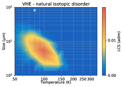
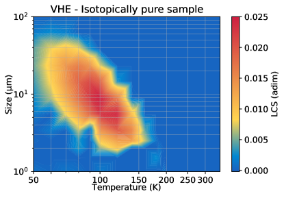
Figure S9: Lattice cooling strength as a function of size, temperature, and isotopic disorder. The lattice cooling strength (S14) is reported as a function of the characteristic size of the rectangle and equilibrium temperature around which the perturbation is applied. The white cross in the upper panel represent the simulation conditions which are closest to the single-spot experiments discussed in Sec. 3 of the Supplementary Material of Ref. [14]—the lack of lattice cooling predicted under these conditions agrees with the experiments. We note that lattice cooling in natural samples (upper panel) is weaker compared to isotopically pure samples (bottom panel).

In this section we discuss how isotopic-mass disorder, size of the sample, and temperature affect the LCS emerging from the VHE in graphite. The effect of isotopic-mass disorder is taken into account by the parameters appearing in the VHE. These were computed from first principles for graphite with natural concentration of isotopes (98.9% ¹²C, 1.1% ¹³C) and for isotopically purified samples (99.9% ¹²C, 0.1% ¹³C), see Sec. VIII for details. The effect of sample size was considered by uniformly rescaling the simulation domain (V.2) and the perturbation (S15). We accounted for grain-boundary scattering as discussed in Ref. [9], considering a grain size of $20\mu m$ that is realistic for high-quality samples [14, 15]. The temperature was monitored in the same point where the perturbation was applied. The effect of equilibrium temperature was taken into account through the temperature dependence of the parameters entering in the viscous heat equations, as shown by Table I in Ref. [9] and Table. 1 at the end of this manuscript.

We show in Fig. S9 that in natural samples lattice cooling is maximized at temperatures around 70-120 K and is significant in devices having size 5-20 $\mu m$. Importantly, LCS becomes negligible in devices having size larger than 30 $\mu m$. We note that Ref. [14] performed pump-probe experiments in graphite using heaters with radius equal to 6 $\mu m$ (details are reported in the Supplementary Material of that reference). When we used a simulation setup similar to the experiments of Ref. [14], i.e. $\sigma_{x}=6\mu m$ in Eq. (S15) and simulation boundaries separated by a large distance (80 $\mu m$), we did not find temperature oscillations (LCS=0 in the point highlighted with the white cross in the upper panel of Fig. S9), in agreement with the experiments of Ref. [14]. We also simulated the ring-shaped geometry used by Jeong et al. [14], finding very good agreement between the theoretical relaxation timescales and the experimental ones, as we will show in Sec. VII.

VI Comparison between viscous, inviscid, and diffusive relaxation

VI.1 Inviscid (DPLE) relaxation

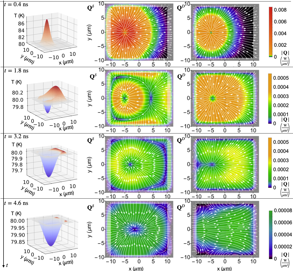
Figure S10: Transient hydrodynamic heat backflow and lattice cooling in the DPLE (inviscid) limit. We show the DPLE predictions for the relaxation in time of a temperature perturbation (obtained applying a localized heater to a device in the time interval from 0 to 0.4 ns) in a graphitic device thermalised at 80 K the boundaries (thermalisation occurs in shaded regions, see SM V.1). Rows show different instants in time for temperature (left column), temperature-gradient heat-flux component ($\bm{Q}^{\delta}$, central column), and drifting heat-flux component ($\bm{Q}^{D}$, right column). The emergence of lattice cooling, i.e. a temperature locally and transiently lower than the initial value $T{=}80$ K, is evident and originates from the lagged coupled evolution of $\bm{Q}^{\delta}$ and $\bm{Q}^{D}$.

In this section we discuss how the thermal viscosity affects temperature oscillations. Fig. S10 shows that solving the viscous heat equations in the inviscid limit ($\mu=0$)—which is analytically equivalent to solving the DPLE equation, see Sec. I—yields temperature oscillations with a higher magnitude compared to those obtained in the case of the viscous heat equations (Fig. 2). Therefore, Fig. S10 shows that a finite viscosity is not necessary to observe transient heat backflow, since a lagged response between temperature gradient and heat flux can emerge also in the inviscid limit, as detailed in Sec. I. However, we will show later in Sec. VII that accounting for the thermal viscous is needed to obtain quantitative agreement between the relaxation timescales predicted from theory and those measured in experiments [14]. Fig. 4 in the main text discusses how accounting for thermal viscosity is necessary to capture lengthscales at which hydrodynamic behavior was observed by Huberman et al. [16] and Ding et al. [15].

VI.2 Diffusive (Fourier) relaxation

We show in Fig. S11 that temperature oscillations do not emerge from Fourier’s law. This behavior was trivially expected from an analytical analysis of Fourier’s diffusive equation, $C\frac{\partial T}{\partial t}{-}\sum_{ij}\kappa^{ij}\frac{\partial^{2}T}{\partial r^{i}r^{y}}=0$, whose smoothing property [17] implies that the evolution of a positive temperature perturbation relaxes to equilibrium decaying in a monotonic way. Also, within Fourier’s law the heat flux has one single component proportional to the temperature gradient, so heat backflow is impossible.

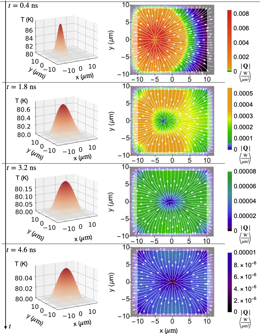
Figure S11: Temporal evolution of a localized temperature perturbation according to Fourier’s law. Rows show different instants in time for the temperature profile (left) and heat flux (right).

VI.3 Comparing VHE, DPLE & Fourier’s relaxations

The device geometry, the transient perturbation, and the boundary conditions used in Figs. 2,S10,S11 are exactly the same. In Fig. S12, we compare the predictions from the viscous VHE, the inviscid DPLE, and the diffusive Fourier’s law for the evolution in time of the temperature in the point $\bm{r}_{c}{=}(5\mu m,0\mu m$), where the temperature perturbation is centered. We see that both DPLE and VHE yield a wave-like relaxation for temperature, the inviscid (DPLE) relaxation is faster and yields stronger oscillatory behavior compared to the VHE relaxation. In contrast, an oscillatory relaxation for temperature is absent in Fourier’s law.

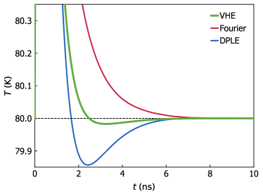
Figure S12: Temperature relaxation from VHE, DPLE, and Fourier’s law. The temporal evolution of the temperature in the center ($5\mu m,0\mu m$) of the external heat source (switched off at t=0.4 ns, see text for details) is shown in red for Fourier’s law, in blue for the DPLE, and in green for the VHE. Temperature oscillations are visible both in the viscous VHE and inviscid DPLE cases (with a larger amplitude in the inviscid case), and are absent in Fourier’s law.

VII Lattice cooling in a ring-shaped geometry

In this section we simulate a ring-shaped perturbation, representing the experimental setup by Jeong et al. [14]. We use a 15-$\mu m$-diameter ring-shape pump, with Gaussian profile having full width at half a maximum equal to $3\ \mathrm{\mu m}$ (these values were confirmed also by analyzing Fig. 1c in Ref. [14]):

$$\dot{q}(\bm{r},t){=}\mathcal{H}\;\theta(t_{\rm heat}{-}t)\exp\left[-\tfrac{(|\bm{r}|-r_{\rm{heater}})^{2}}{2\sigma_{r}^{2}}\right].$$ (S16)

We used a circular simulation domain with diameter equal to $30\ \mathrm{\mu m}$. We simulated thermalisation with an external heat bath happening in the annular region having inner diameter $20\ \mathrm{\mu m}$ and the outer diameter equal to $30\ \mathrm{\mu m}$, using the approach to describe thermalisation with the environment in a realistic way discussed in Sec. V.1. We used the parameters for graphite at natural isotopic concentration (computed from first-principles and reported in Table I of Ref. [9]), considering a grain size of $20\mu m$ (estimated from the largest grains in Fig. S1 of Ref. [14]).

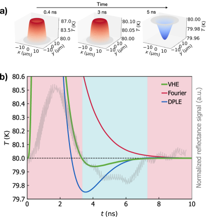
Figure S13: Lattice cooling in a ring-shaped geometry. a), time evolution of the temperature profile from the viscous heat equations. b), evolution of the temperature measured in the center of the ring obtained from the VHE (green), DPLE (blue), or Fourier (red). Grey, normalized reflectance measured by Jeong et al. [14] (grey); the sign of the normalized reflectance signal is indicated by the background color: red is positive and blue is negative. The experimental relaxation timescale, i.e. the time instant at which the normalized reflectance signal becomes lower than the initial value, is in agreement with the relaxation timescale predicted by the VHE (see text).

The ring-shaped perturbation was applied for $0.4\ ns$ and then switched off, as in the experiments. We report in Fig. S13 the temporal evolution of the temperature measured in the center of the ring, computed from the viscous VHE, the inviscid DPLE, and from Fourier’s law. The relaxation timescales emerging from the VHE match the experimental relaxation timescales discussed by Jeong et al. [14]. In particular, we note that the time at which the normalised reflectance signal changes sign matches the time at which the temperature computed by the VHE changes sign. In contrast, the DPLE (i.e. the VHE with $\mu=0$) predict the relaxation to be faster than that observed in experiments. We conclude by noting that the pioneering experiments of Ref. [14] showed a non-negligible noise in the normalized reflectance signal (see Fig. 2 in Ref. [14]) and for this reason they focused exclusively on the sign of the normalized reflectance (shown by the background color in Fig. S13) rather than on the absolute reflectance values. For these reasons, we focused on comparing the times at which $T(\bm{r},t)-T_{eq}$ changes sign, and the time at which the experimental normalized reflectance changes sign. Our results suggest that it is necessary to account for the thermal viscosity in order to obtain agreement between the experimental and theoretical timescales that characterize lattice cooling.

VIII Parameters entering the viscous heat equations

In order to simplify the notation for the paramenters entering in the viscous heat equations (1,2), we defined the following parameters: $\alpha^{ji}{=}W_{0j}^{i}\sqrt{\overline{T}A^{j}C}$, $\beta^{ij}{=}\sqrt{\frac{CA^{i}}{\overline{T}}}W_{i0}^{j}$, $\gamma^{ij}{=}\sqrt{A^{i}A^{j}}D_{U}^{ij}$. In these expressions, $C$ is the specific heat, ${W}_{0j}^{i}$ is the velocity tensor that arises from the non-diagonal form of the diffusion operator in the basis of the eigenvectors of the normal part of the scattering matrix, $\bar{T}$ is the reference (equilibrium) temperature on which a perturbation is applied, $A^{i}$ is the specific momentum in direction $i$. More details on these parameters can be found in Ref. [9].

VIII.1 Graphite

Table 1: Parameters entering the viscous heat equations for isotopically purified graphite (99.9 % ¹²C, 0.1 % ¹³C). We report here only the in-plane components of the tensors needed to perform the calculations: $\kappa^{ij}_{\rm P}=\kappa_{\rm P}\delta^{ij}$, $\kappa^{ij}_{\rm C}=\kappa_{\rm C}\delta^{ij}$ (see Refs. [18, 19, 20, 21] for details on $\kappa_{\rm C}$), $K^{ij}_{S}=K_{S}\delta^{ij}$, ${D}_{U,{\rm bulk}}^{ij}={D}_{U,{\rm bulk}}\delta^{ij}$, ${F}_{U}^{ij}={F}_{U}\delta^{ij}$, $A=A^{i}\;\forall\;i$, $W^{j}_{0i}=W^{j}_{i0}=W\delta^{ij}$, where the indexes $i,j$ represent the in-plane directions $x,y$ only ($i,j=1,2$ and $i\neq j$).

T [K]	$\kappa_{\rm P}\;\big{[}\rm\frac{W}{m{\cdot}K}\big{]}$	$\kappa_{\rm C}\;\big{[}\rm\frac{W}{m{\cdot}K}\big{]}$	${K_{S}\;\big{[}\rm\frac{W}{m^{2}{\cdot}K}\big{]}}$	$\mu^{iiii}_{\rm bulk}\;[\rm Pa{\cdot}s]$	$\mu^{ijij}_{\rm bulk}\;[\rm Pa{\cdot}s]$	$\mu^{ijji}_{\rm bulk}\;[\rm Pa{\cdot}s]$	$M^{iiii}\;[\rm\frac{Pa{\cdot}s}{m}]$	$M^{ijij}\;[\rm\frac{Pa{\cdot}s}{m}]$	$M^{ijji}\;[\rm\frac{Pa{\cdot}s}{m}]$	${D}_{U,{\rm bulk}}\;[\rm ns^{-1}]$	${F}_{U}\;[\rm\frac{m}{s}]$	A $\big{[}\rm\frac{pg}{\mu m^{3}}\big{]}$	$C$ $\big{[}\rm\frac{pg}{\mu m{\cdot}ns^{2}{\cdot}K}\big{]}$	W $\big{[}\rm\frac{\mu m}{ns}\big{]}$
50	3.34175e+04	8.17849e-05	2.57075e+08	1.11244e-03	5.62103e-04	2.71810e-04	4.39176e+02	1.46638e+02	1.46269e+02	2.41659e-02	4.26877e+03	1.53433e-04	1.00900e-04	2.72761e+00
60	3.52935e+04	1.44119e-04	3.95197e+08	1.09365e-03	5.84333e-04	2.51162e-04	7.15578e+02	2.39244e+02	2.38166e+02	4.34202e-02	4.59801e+03	2.29498e-04	1.41101e-04	3.00647e+00
70	3.24978e+04	2.40448e-04	5.59073e+08	1.09700e-03	6.15163e-04	2.37329e-04	1.07264e+03	3.59308e+02	3.56661e+02	8.50411e-02	4.88642e+03	3.20256e-04	1.84524e-04	3.25249e+00
80	2.74850e+04	4.06335e-04	7.45726e+08	1.11813e-03	6.50051e-04	2.30398e-04	1.51011e+03	5.07190e+02	5.01440e+02	1.68503e-01	5.13608e+03	4.25102e-04	2.30997e-04	3.45924e+00
90	2.25348e+04	7.19062e-04	9.52361e+08	1.15613e-03	6.86615e-04	2.31108e-04	2.02532e+03	6.82641e+02	6.71286e+02	3.18608e-01	5.34894e+03	5.43532e-04	2.80534e-04	3.62371e+00
100	1.84465e+04	1.30478e-03	1.17648e+09	1.21344e-03	7.23418e-04	2.41404e-04	2.61392e+03	8.85021e+02	8.64331e+02	5.63474e-01	5.52812e+03	6.75030e-04	3.33160e-04	3.74625e+00
120	1.27814e+04	3.97919e-03	1.66857e+09	1.39850e-03	7.94571e-04	2.98592e-04	3.98943e+03	1.36695e+03	1.31087e+03	1.45053e+00	5.80204e+03	9.74775e-04	4.47442e-04	3.88006e+00
140	9.33971e+03	9.87325e-03	2.20653e+09	1.67560e-03	8.59931e-04	4.04889e-04	5.59088e+03	1.94459e+03	1.82232e+03	3.02867e+00	5.99201e+03	1.31862e-03	5.72512e-04	3.90257e+00
160	7.14426e+03	2.01725e-02	2.77638e+09	2.00642e-03	9.18230e-04	5.41712e-04	7.37504e+03	2.60822e+03	2.38191e+03	5.43535e+00	6.12653e+03	1.70002e-03	7.05946e-04	3.85826e+00
180	5.66903e+03	3.55200e-02	3.36529e+09	2.33991e-03	9.69102e-04	6.83651e-04	9.30496e+03	3.34736e+03	2.97640e+03	8.74395e+00	6.22525e+03	2.11243e-03	8.44946e-04	3.78035e+00
185	5.37644e+03	4.01659e-02	3.51416e+09	2.41895e-03	9.80665e-04	7.17548e-04	9.80654e+03	3.54269e+03	3.12927e+03	9.71528e+00	6.24592e+03	2.21967e-03	8.80257e-04	3.75825e+00
190	5.10779e+03	4.51306e-02	3.66336e+09	2.49541e-03	9.91776e-04	7.50384e-04	1.03149e+04	3.74191e+03	3.28357e+03	1.07442e+01	6.26529e+03	2.32838e-03	9.15719e-04	3.73558e+00
195	4.86054e+03	5.04083e-02	3.81277e+09	2.56902e-03	1.00244e-03	7.82019e-04	1.08297e+04	3.94485e+03	3.43919e+03	1.18304e+01	6.28349e+03	2.43848e-03	9.51302e-04	3.71251e+00
200	4.63247e+03	5.59919e-02	3.96223e+09	2.63960e-03	1.01267e-03	8.12350e-04	1.13505e+04	4.15136e+03	3.59604e+03	1.29735e+01	6.30063e+03	2.54990e-03	9.86974e-04	3.68920e+00
220	3.87676e+03	8.11890e-02	4.55837e+09	2.88966e-03	1.04937e-03	9.19634e-04	1.34874e+04	5.01005e+03	4.23388e+03	1.80998e+01	6.36031e+03	3.00734e-03	1.13005e-03	3.59566e+00
240	3.30876e+03	1.10363e-01	5.14699e+09	3.08900e-03	1.07987e-03	1.00459e-03	1.56967e+04	5.91420e+03	4.88503e+03	2.40671e+01	6.40897e+03	3.48061e-03	1.27276e-03	3.50487e+00
260	2.87089e+03	1.42551e-01	5.72314e+09	3.24372e-03	1.10492e-03	1.06990e-03	1.79634e+04	6.85568e+03	5.54605e+03	3.07981e+01	6.44952e+03	3.96638e-03	1.41411e-03	3.41888e+00
280	2.52599e+03	1.76706e-01	6.28327e+09	3.36215e-03	1.12530e-03	1.11933e-03	2.02756e+04	7.82758e+03	6.21450e+03	3.82043e+01	6.48385e+03	4.46204e-03	1.55341e-03	3.33828e+00
300	2.24925e+03	2.11805e-01	6.82487e+09	3.45227e-03	1.14175e-03	1.15650e-03	2.26238e+04	8.82402e+03	6.88860e+03	4.61938e+01	6.51324e+03	4.96554e-03	1.69010e-03	3.26300e+00
350	1.75530e+03	2.98054e-01	8.08784e+09	3.59424e-03	1.16993e-03	1.21399e-03	2.86057e+04	1.13924e+04	8.59059e+03	6.81463e+01	6.57048e+03	6.24865e-03	2.01775e-03	3.09612e+00
400	1.43431e+03	3.74983e-01	9.21271e+09	3.66698e-03	1.18574e-03	1.24278e-03	3.46848e+04	1.40297e+04	1.03064e+04	9.20012e+01	6.61114e+03	7.55350e-03	2.32135e-03	2.95575e+00

All the parameters for graphite were computed from first principles, see Ref. [9] for computational details. The parameters for graphite with natural-abundance isotopic-mass disorder (98.9 % ¹²C, 1.1 % ¹³C) are reported in Table I of Ref. [9]. The parameters for isotopically pure samples (99.9 % ¹²C, 0.1 % ¹³C) are reported in Table. 1. We conclude by noting that in this work we employed the approximation of considering the parameters entering in the VHE, DPLE, and Fourier’s equation to be independent from frequency. This approximation is realistic in the MHz range considered here, as discussed by Ref. [22].

VIII.2 Monoisotopic hexagonal boron nitride

First-principles calculations have been performed with the Quantum ESPRESSO distribution [23, 24] using the the local-density approximation (LDA) for the exchange-correlation energy functional, since it has been shown to accurately describe the vibrational and thermal properties of hBN [25, 26, 27]. The pseudopotentials have been taken from the pseudo Dojo library [28] (specifically, we have used norm-conserving and scalar-relativistic pseudopotentials with accuracy “stringent” and of type ONCVPSP v0.4). The crystal structure of hBN has been taken from [29] (Crystallographic Open Database  [30] id 2016170). Kinetic energy cutoffs of 90 and 360 Ry have been used for the wave functions and for the charge density; the Brillouin zone (BZ) is integrated with a Monkhorst-Pack mesh of $8{\times}8{\times}3$ points, with a (1,1,1) shift. The equilibrium crystal structure has been computed performing a “vc-relax” calculation with Quantum ESPRESSO and the DFT-optimized lattice parameters are $a=2.489089$ Å and $c/a=2.604045$. Second-order force constants have been computed on a $8{\times}8{\times}3$ mesh using density-functional perturbation theory  [31] and accounting for the non-analytic term correction due to the dielectric tensor and Born effective charges. Third-order force constants have been computed using the finite-difference method implemented in ShengBTE [32], on a $4{\times}4{\times}2$ supercell, integrating the BZ with a $2{\times}2{\times}1$ Monkhorst-Pack mesh, and considering interactions up to 3.944 Å (which corresponds to the 6th nearest neighbor). Then, anharmonic force constants have been converted from ShengBTE format to mat3R format using the interconversion software d3_import_shengbte.x provided with the D3Q package  [33, 34], including interactions up to the second neighbouring cell for the re-centering of the third-order force constants (parameter NFAR=2). All the parameters entering in the VHE have been computed using a q-point mesh equal to $49{\times}49{\times}3$ and a Gaussian smearing of $6\;{\rm cm}^{-1}$, and are reported in Table 2.

Table 2: Parameters entering the viscous heat equations for h¹¹BN. We report here only the in-plane components of the tensors needed to perform the calculations: $\kappa^{ij}_{\rm P}=\kappa_{\rm P}\delta^{ij}$, $\kappa^{ij}_{\rm C}=\kappa_{\rm C}\delta^{ij}$, $K^{ij}_{S}=K_{S}\delta^{ij}$, ${D}_{U,{\rm bulk}}^{ij}={D}_{U,{\rm bulk}}\delta^{ij}$, ${F}_{U}^{ij}={F}_{U}\delta^{ij}$, $A=A^{i}\;\forall\;i$, $W^{j}_{0i}=W^{j}_{i0}=W\delta^{ij}$, where the indexes $i,j$ represent the in-plane directions $x,y$ only ($i,j=1,2$ and $i\neq j$).

T [K]	$\kappa_{\rm P}\;\big{[}\rm\frac{W}{m{\cdot}K}\big{]}$	$\kappa_{\rm C}\;\big{[}\rm\frac{W}{m{\cdot}K}\big{]}$	${K_{S}\;\big{[}\rm\frac{W}{m^{2}{\cdot}K}\big{]}}$	$\mu^{iiii}_{\rm bulk}\;[\rm Pa{\cdot}s]$	$\mu^{ijij}_{\rm bulk}\;[\rm Pa{\cdot}s]$	$\mu^{ijji}_{\rm bulk}\;[\rm Pa{\cdot}s]$	$M^{iiii}\;[\rm\frac{Pa{\cdot}s}{m}]$	$M^{ijij}\;[\rm\frac{Pa{\cdot}s}{m}]$	$M^{ijji}\;[\rm\frac{Pa{\cdot}s}{m}]$	${D}_{U,{\rm bulk}}\;[\rm ns^{-1}]$	${F}_{U}\;[\rm\frac{m}{s}]$	A $\big{[}\rm\frac{pg}{\mu m^{3}}\big{]}$	$C$ $\big{[}\rm\frac{pg}{\mu m{\cdot}ns^{2}{\cdot}K}\big{]}$	W $\big{[}\rm\frac{\mu m}{ns}\big{]}$
50	5.08496e+03	4.39299e-04	3.18233e+08	7.09609e-04	4.61623e-04	1.24381e-04	6.97634e+02	2.33387e+02	2.32121e+02	3.15987e-01	3.70983e+03	2.73574e-04	1.49113e-04	2.40299e+00
60	3.94420e+03	6.91660e-04	4.77290e+08	7.07393e-04	4.76252e-04	1.16007e-04	1.15258e+03	3.86399e+02	3.83081e+02	7.48719e-01	3.87655e+03	4.26806e-04	2.08230e-04	2.56422e+00
75	2.87382e+03	1.19669e-03	7.48233e+08	7.07296e-04	4.91045e-04	1.08615e-04	2.04154e+03	6.87240e+02	6.77105e+02	1.93310e+00	4.01963e+03	7.19449e-04	3.03986e-04	2.71119e+00
100	1.89907e+03	2.58860e-03	1.24792e+09	7.20155e-04	4.98382e-04	1.11402e-04	3.92792e+03	1.33705e+03	1.29525e+03	5.71441e+00	4.10962e+03	1.33990e-03	4.71727e-04	2.79944e+00
125	1.37164e+03	5.21646e-03	1.78806e+09	7.79727e-04	5.01978e-04	1.39347e-04	6.13109e+03	2.12395e+03	2.00311e+03	1.19136e+01	4.14080e+03	2.07076e-03	6.44647e-04	2.78843e+00
150	1.06699e+03	9.66905e-03	2.36077e+09	8.91251e-04	5.12533e-04	1.89739e-04	8.52906e+03	3.02013e+03	2.75353e+03	2.02022e+01	4.16302e+03	2.86999e-03	8.22855e-04	2.73368e+00
175	8.83008e+02	1.62740e-02	2.95342e+09	1.02915e-03	5.30428e-04	2.49625e-04	1.10622e+04	4.00902e+03	3.52496e+03	3.01303e+01	4.18665e+03	3.71435e-03	1.00492e-03	2.66425e+00
200	7.65123e+02	2.51062e-02	3.55061e+09	1.16741e-03	5.52319e-04	3.07683e-04	1.36961e+04	5.07502e+03	4.30804e+03	4.13328e+01	4.21210e+03	4.58997e-03	1.18813e-03	2.59391e+00
225	6.83803e+02	3.60584e-02	4.13896e+09	1.29214e-03	5.74869e-04	3.58660e-04	1.64072e+04	6.20280e+03	5.09861e+03	5.35343e+01	4.23792e+03	5.48778e-03	1.37008e-03	2.52756e+00
250	6.23329e+02	4.88988e-02	4.70873e+09	1.39919e-03	5.95930e-04	4.01553e-04	1.91773e+04	7.37844e+03	5.89459e+03	6.65173e+01	4.26281e+03	6.40150e-03	1.54901e-03	2.46616e+00
275	5.75413e+02	6.33176e-02	5.25353e+09	1.48916e-03	6.14491e-04	4.37170e-04	2.19921e+04	8.59015e+03	6.69477e+03	8.01021e+01	4.28596e+03	7.32669e-03	1.72367e-03	2.40940e+00
300	5.35638e+02	7.89685e-02	5.76951e+09	1.56429e-03	6.30300e-04	4.66758e-04	2.48404e+04	9.82843e+03	7.49827e+03	9.41385e+01	4.30696e+03	8.26014e-03	1.89306e-03	2.35678e+00
325	5.01567e+02	9.55019e-02	6.25468e+09	1.62704e-03	6.43502e-04	4.91475e-04	2.77130e+04	1.10858e+04	8.30433e+03	1.08503e+02	4.32573e+03	9.19946e-03	2.05633e-03	2.30792e+00
350	4.71776e+02	1.12591e-01	6.70835e+09	1.67963e-03	6.54418e-04	5.12263e-04	3.06029e+04	1.23564e+04	9.11232e+03	1.23095e+02	4.34233e+03	1.01428e-02	2.21279e-03	2.26256e+00

References

- Schmidt et al. [2008] A. J. Schmidt, X. Chen, and G. Chen, Pulse accumulation, radial heat conduction, and anisotropic thermal conductivity in pump-probe transient thermoreflectance, Rev. Sci. Instrum. 79, 114902 (2008).
- Balandin [2011] A. A. Balandin, Thermal properties of graphene and nanostructured carbon materials, Nat. Mater. 10, 569 (2011).
- Fugallo et al. [2014] G. Fugallo, A. Cepellotti, L. Paulatto, M. Lazzeri, N. Marzari, and F. Mauri, Thermal Conductivity of Graphene and Graphite: Collective Excitations and Mean Free Paths, Nano Lett. 14, 6109 (2014).
- Machida et al. [2020] Y. Machida, N. Matsumoto, T. Isono, and K. Behnia, Phonon hydrodynamics and ultrahigh–room-temperature thermal conductivity in thin graphite, Science 367, 309 (2020).
- Jiang et al. [2018] P. Jiang, X. Qian, R. Yang, and L. Lindsay, Anisotropic thermal transport in bulk hexagonal boron nitride, Phys. Rev. Materials 2, 064005 (2018).
- Yuan et al. [2019] C. Yuan, J. Li, L. Lindsay, D. Cherns, J. W. Pomeroy, S. Liu, J. H. Edgar, and M. Kuball, Modulating the thermal conductivity in hexagonal boron nitride via controlled boron isotope concentration, Commun. Phys. 2 (2019).
- Qian et al. [2021] X. Qian, J. Zhou, and G. Chen, Phonon-engineered extreme thermal conductivity materials, Nat. Mater. 20, 1188 (2021).
- Moon et al. [2023] S. Moon, J. Kim, J. Park, S. Im, J. Kim, I. Hwang, and J. K. Kim, Hexagonal Boron Nitride for Next-Generation Photonics and Electronics, Adv. Mater. 35, 2204161 (2023).
- Chen [2021] G. Chen, Non-Fourier phonon heat conduction at the microscale and nanoscale, Nat. Rev. Phys. 3, 555 (2021).
- Huang et al. [2023] X. Huang, Y. Guo, Y. Wu, S. Masubuchi, K. Watanabe, T. Taniguchi, Z. Zhang, S. Volz, T. Machida, and M. Nomura, Observation of phonon Poiseuille flow in isotopically purified graphite ribbons, Nat. Commun. 14, 2044 (2023).
- Huberman et al. [2019] S. Huberman, R. A. Duncan, K. Chen, B. Song, V. Chiloyan, Z. Ding, A. A. Maznev, G. Chen, and K. A. Nelson, Observation of second sound in graphite at temperatures above 100 K, Science 364, 375 (2019).
- Jeong et al. [2021] J. Jeong, X. Li, S. Lee, L. Shi, and Y. Wang, Transient hydrodynamic lattice cooling by picosecond laser irradiation of graphite, Phys. Rev. Lett. 127, 085901 (2021).
- Ding et al. [2022] Z. Ding, K. Chen, B. Song, J. Shin, A. A. Maznev, K. A. Nelson, and G. Chen, Observation of second sound in graphite over 200 k, Nat. Commun. 13, 285 (2022).
- Note [1] Specifically, Ref. [15] observed temperature oscillations at temperatures as high as 200 K in isotopically purified graphite, while the pioneering works [16, 14] observed temperature oscillations around 80-100 K in graphite at natural isotopic abundance.
- Peierls [1955] R. E. Peierls, Quantum theory of solids (Oxford university press, 1955).
- Lindsay et al. [2019] L. Lindsay, A. Katre, A. Cepellotti, and N. Mingo, Perspective on ab initio phonon thermal transport, J. Appl. Phys. 126, 050902 (2019).
- Chaput [2013] L. Chaput, Direct Solution to the Linearized Phonon Boltzmann Equation, Phys. Rev. Lett. 110, 265506 (2013).
- Fugallo et al. [2013] G. Fugallo, M. Lazzeri, L. Paulatto, and F. Mauri, Ab initio variational approach for evaluating lattice thermal conductivity, Phys. Rev. B 88, 045430 (2013).
- Lee et al. [2015] S. Lee, D. Broido, K. Esfarjani, and G. Chen, Hydrodynamic phonon transport in suspended graphene, Nat. Commun. 6, 6290 (2015).
- Cepellotti and Marzari [2016] A. Cepellotti and N. Marzari, Thermal Transport in Crystals as a Kinetic Theory of Relaxons, Phys. Rev. X 6, 041013 (2016).
- Ding et al. [2018] Z. Ding, J. Zhou, B. Song, V. Chiloyan, M. Li, T.-H. Liu, and G. Chen, Phonon hydrodynamic heat conduction and knudsen minimum in graphite, Nano Lett. 18, 638 (2018).
- Guo et al. [2021a] Y. Guo, Z. Zhang, M. Bescond, S. Xiong, M. Wang, M. Nomura, and S. Volz, Size effect on phonon hydrodynamics in graphite microstructures and nanostructures, Phys. Rev. B 104, 075450 (2021a).
- Li et al. [2022] X. Li, H. Lee, E. Ou, S. Lee, and L. Shi, Reexamination of hydrodynamic phonon transport in thin graphite, J. Appl. Phys. 131, 075104 (2022).
- Huang et al. [2022] X. Huang, Y. Guo, S. Volz, and M. Nomura, Mapping phonon hydrodynamic strength in micrometer-scale graphite structures, Appl. Phys. Express 15, 105001 (2022).
- Cepellotti et al. [2015] A. Cepellotti, G. Fugallo, L. Paulatto, M. Lazzeri, F. Mauri, and N. Marzari, Phonon hydrodynamics in two-dimensional materials, Nat. Commun. 6, 6400 (2015).
- Majee and Aksamija [2018] A. K. Majee and Z. Aksamija, Dynamical thermal conductivity of suspended graphene ribbons in the hydrodynamic regime, Phys. Rev. B 98, 024303 (2018).
- Raya-Moreno et al. [2022] M. Raya-Moreno, J. Carrete, and X. Cartoixà, Hydrodynamic signatures in thermal transport in devices based on two-dimensional materials: An ab initio study, Phys. Rev. B 106, 014308 (2022).
- Guo et al. [2021b] Y. Guo, Z. Zhang, M. Nomura, S. Volz, and M. Wang, Phonon vortex dynamics in graphene ribbon by solving Boltzmann transport equation with ab initio scattering rates, Int. J. Heat Mass Transf. 169, 120981 (2021b).
- Zhang et al. [2022] C. Zhang, S. Huberman, and L. Wu, On the emergence of heat waves in the transient thermal grating geometry, J. Appl. Phys. 132, 085103 (2022).
- Han and Ruan [2023] Z. Han and X. Ruan, Is Thermal Conductivity of Graphene Divergent and Higher Than Diamond?, arXiv: 2302.12216 (2023).
- Cepellotti and Marzari [2017a] A. Cepellotti and N. Marzari, Boltzmann Transport in Nanostructures as a Friction Effect, Nano Lett. 17, 4675 (2017a).
- Machida et al. [2018] Y. Machida, A. Subedi, K. Akiba, A. Miyake, M. Tokunaga, Y. Akahama, K. Izawa, and K. Behnia, Observation of Poiseuille flow of phonons in black phosphorus, Sci. Adv. 4, eaat3374 (2018).
- Sendra et al. [2022] L. Sendra, A. Beardo, J. Bafaluy, P. Torres, F. X. Alvarez, and J. Camacho, Hydrodynamic heat transport in dielectric crystals in the collective limit and the drifting/driftless velocity conundrum, Phys. Rev. B 106, 155301 (2022).
- Li and Lee [2018] X. Li and S. Lee, Role of hydrodynamic viscosity on phonon transport in suspended graphene, Phys. Rev. B 97, 094309 (2018).
- Guo et al. [2018] Y. Guo, D. Jou, and M. Wang, Nonequilibrium thermodynamics of phonon hydrodynamic model for nanoscale heat transport, Phys. Rev. B 98, 104304 (2018).
- Shang et al. [2020] M.-Y. Shang, C. Zhang, Z. Guo, and J.-T. Lü, Heat vortex in hydrodynamic phonon transport of two-dimensional materials, Sci. Rep. 10, 8272 (2020).
- Simoncelli et al. [2020] M. Simoncelli, N. Marzari, and A. Cepellotti, Generalization of fourier’s law into viscous heat equations, Phys. Rev. X 10, 011019 (2020).
- Sendra et al. [2021] L. Sendra, A. Beardo, P. Torres, J. Bafaluy, F. X. Alvarez, and J. Camacho, Derivation of a hydrodynamic heat equation from the phonon Boltzmann equation for general semiconductors, Phys. Rev. B 103, L140301 (2021).
- Joseph and Preziosi [1989] D. D. Joseph and L. Preziosi, Heat waves, Rev. Mod. Phys. 61, 41 (1989).
- Tzou [1995] D. Y. Tzou, A Unified Field Approach for Heat Conduction From Macro- to Micro-Scales, J Heat Transf 117, 8 (1995).
- Cattaneo [1958] C. Cattaneo, A form of heat-conduction equations which eliminates the paradox of instantaneous propagation, Comptes Rendus 247, 431 (1958).
- Note [2] In order to simplify the notation, here we defined , , , where is the temperature at which thermal conductivity and viscosity are determined, is the velocity tensor arising from the non-diagonal form of the diffusion operator in the basis of the eigenvectors of the normal part of the scattering matrix discussed in Ref. [9], and the Umklapp-dissipation timescale discussed in Ref. [9].
- Note [3] We investigate monoisotopic h11BN because Refs. [27, 81] suggest that head hydrodynamics in h11BN is stronger than in hexagonal boron nitride with natural isotopic-mass disorder (19.9% 10B and 80.1% 11B).
- Aharon-Steinberg et al. [2022] A. Aharon-Steinberg, T. Völkl, A. Kaplan, A. K. Pariari, I. Roy, T. Holder, Y. Wolf, A. Y. Meltzer, Y. Myasoedov, M. E. Huber, B. Yan, G. Falkovich, L. S. Levitov, M. Hücker, and E. Zeldov, Direct observation of vortices in an electron fluid, Nature 607, 74 (2022).
- Menges et al. [2016] F. Menges, H. Riel, A. Stemmer, and B. Gotsmann, Nanoscale thermometry by scanning thermal microscopy, Rev. Sci. Instrum. 87, 074902 (2016).
- Cheng et al. [2022] Z. Cheng, X. Ji, and D. G. Cahill, Battery absorbs heat during charging uncovered by ultra-sensitive thermometry, J. Power Sources 518, 230762 (2022).
- Cahill et al. [2014] D. G. Cahill, P. V. Braun, G. Chen, D. R. Clarke, S. Fan, K. E. Goodson, P. Keblinski, W. P. King, G. D. Mahan, A. Majumdar, H. J. Maris, S. R. Phillpot, E. Pop, and L. Shi, Nanoscale thermal transport. II. 2003–2012, Appl. Phys. Rev. 1, 011305 (2014).
- Braun et al. [2022] O. Braun, R. Furrer, P. Butti, K. Thodkar, I. Shorubalko, I. Zardo, M. Calame, and M. L. Perrin, Spatially mapping thermal transport in graphene by an opto-thermal method, NPJ 2D Mater. Appl. 6, 1 (2022).
- Ziabari et al. [2018] A. Ziabari, P. Torres, B. Vermeersch, Y. Xuan, X. Cartoixà, A. Torelló, J.-H. Bahk, Y. R. Koh, M. Parsa, P. D. Ye, F. X. Alvarez, and A. Shakouri, Full-field thermal imaging of quasiballistic crosstalk reduction in nanoscale devices, Nat. Commun. 9, 255 (2018).
- Note [4] We recall that the curl of a gradient is zero, thus Fourier’s heat flux is irrotational.
- Ziman [1960] J. M. Ziman, Electrons and phonons: the theory of transport phenomena in solids (Oxford university press, 1960).
- Ravichandran et al. [2018] N. K. Ravichandran, H. Zhang, and A. J. Minnich, Spectrally Resolved Specular Reflections of Thermal Phonons from Atomically Rough Surfaces, Phys. Rev. X 8, 041004 (2018).
- Note [5] From a mathematical viewpoint, slipping boundaries correspond to having drift-velocity component orthogonal to the boundary equal to zero while allowing the component parallel to the boundary to be non-zero.
- Cepellotti and Marzari [2017b] A. Cepellotti and N. Marzari, Transport waves as crystal excitations, Phys. Rev. Materials 1, 045406 (2017b).
- Zhang and Guo [2021] C. Zhang and Z. Guo, A transient heat conduction phenomenon to distinguish the hydrodynamic and (quasi) ballistic phonon transport, Int. J. Heat Mass Transf. 181, 121847 (2021).
- Xu and Wang [2002] M. Xu and L. Wang, Thermal oscillation and resonance in dual-phase-lagging heat conduction, Int. J. Heat Mass Transf. 45, 1055 (2002).
- Ordóñez-Miranda and Alvarado-Gil [2010] J. Ordóñez-Miranda and J. J. Alvarado-Gil, Exact solution of the dual-phase-lag heat conduction model for a one-dimensional system excited with a periodic heat source, Mech. Res. Commun. 37, 276 (2010).
- Kang et al. [2017] Z. Kang, P. Zhu, D. Gui, and L. Wang, A method for predicting thermal waves in dual-phase-lag heat conduction, Int. J. Heat Mass Transf. 115, 250 (2017).
- Gandolfi et al. [2019] M. Gandolfi, G. Benetti, C. Glorieux, C. Giannetti, and F. Banfi, Accessing temperature waves: A dispersion relation perspective, Int. J. Heat Mass Transf. 143, 118553 (2019).
- Xu [2021] M. Xu, Thermal oscillations, second sound and thermal resonance in phonon hydrodynamics, Proc. Math. Phys. Eng. 477, 20200913 (2021).
- Mazza et al. [2021] G. Mazza, M. Gandolfi, M. Capone, F. Banfi, and C. Giannetti, Thermal dynamics and electronic temperature waves in layered correlated materials, Nat. Commun. 12, 6904 (2021).
- Note [6] In this time-dependent simulation we choose an equilibrium temperature of 80 K to match the temperature at which transient hydrodynamic heat propagation has been observed in recent experiments [16, 14].
- foo [a] To ensure that the perturbation created causes variations within 10% of the equilibrium temperature, we used the following parameters: , , , , .
- [64] D. Skinner, Mathematical Methods, University of Cambridge.
- Barletta and Zanchini [1996] A. Barletta and E. Zanchini, Hyperbolic heat conduction and thermal resonances in a cylindrical solid carrying a steady-periodic electric field, Int. J. Heat Mass Transf. 39, 1307 (1996).
- foo [b] We report the length of the longest side, the shortest side is 0.8 times shorter.
- foo [c] Refs. [16, 15] quantified the hydrodynamic strength as the dip depth of the TTG signal, see e.g. Fig. 1a in Ref. [15].
- Note [7] All the simulations shown in Fig. 3 were performed accounting for grain-boundary scattering as in Ref. [9], and considering a grain size of 20 m. This value was estimated considering the largest grains in Fig. S3 of Ref. [16], Fig. S1 of Ref. [14], Fig. S11 of Ref. [15], and Fig. 1e of Ref. [27], which are all in broad agreement with 20 m.
- Note [8] Experiments [15] for isotopically purified graphite are available only at temperatures higher than 100 K, preventing us to compare VHE and DPLE in the low-temperature limit, where Fig. 4a,b show that viscous effects are largest.
- Vool et al. [2021] U. Vool, A. Hamo, G. Varnavides, Y. Wang, T. X. Zhou, N. Kumar, Y. Dovzhenko, Z. Qiu, C. A. C. Garcia, A. T. Pierce, J. Gooth, P. Anikeeva, C. Felser, P. Narang, and A. Yacoby, Imaging phonon-mediated hydrodynamic flow in WTe2, Nat. Phys 17, 1216 (2021).
- Yang et al. [2021] H.-Y. Yang, X. Yao, V. Plisson, S. Mozaffari, J. P. Scheifers, A. F. Savvidou, E. S. Choi, G. T. McCandless, M. F. Padlewski, C. Putzke, P. J. W. Moll, J. Y. Chan, L. Balicas, K. S. Burch, and F. Tafti, Evidence of a coupled electron-phonon liquid in NbGe2, Nat. Commun. 12, 5292 (2021).
- Jaoui et al. [2022] A. Jaoui, A. Gourgout, G. Seyfarth, A. Subedi, T. Lorenz, B. Fauqué, and K. Behnia, Formation of an Electron-Phonon Bifluid in Bulk Antimony, Phys. Rev. X 12, 031023 (2022).
- Huang and Lucas [2021] X. Huang and A. Lucas, Electron-phonon hydrodynamics, Phys. Rev. B 103, 155128 (2021).
- Protik et al. [2022] N. H. Protik, C. Li, M. Pruneda, D. Broido, and P. Ordejón, The elphbolt ab initio solver for the coupled electron-phonon Boltzmann transport equations, NPJ Comput. Mater 8, 28 (2022).
- Levchenko and Schmalian [2020] A. Levchenko and J. Schmalian, Transport properties of strongly coupled electron–phonon liquids, Ann. Phys. 419, 168218 (2020).
- Coulter et al. [2018] J. Coulter, R. Sundararaman, and P. Narang, Microscopic origins of hydrodynamic transport in the type-II Weyl semimetal WP2, Phys. Rev. B 98, 115130 (2018).
- Wei et al. [2022] X.-Y. Wei, O. A. Santos, C. H. S. Lusero, G. E. W. Bauer, J. Ben Youssef, and B. J. van Wees, Giant magnon spin conductivity in ultrathin yttrium iron garnet films, Nat. Mater. , 1352 (2022).
- Rosales et al. [2023] H. D. Rosales, F. A. G. Albarracín, P. Pujol, and L. D. C. Jaubert, Skyrmion fluid and bimeron glass protected by a chiral spin liquid on a kagome lattice, Phys. Rev. Lett. 130, 106703 (2023).
- Bear [2013] J. Bear, Dynamics of fluids in porous media (Courier Corporation, 2013).
- Note [9] We note that the VHE have a mathematical form mathematically analogous to the damped and diffusion-extended Navier-Stokes equations, used to describe rarefied fluids flowing in porous media in isothermal and laminar conditions, with VHE’s temperature mapping to fluid’s pressure and VHE’s drift velocity mapping to fluid velocity. To see this, we highlight how the linear damping term appearing in the second VHE (2) is analogous to the dissipative term appearing in the linearized “damped” Navier-Stokes equations [82, 83, 84, 85, 86] used e.g. to describe a fluid flowing through a porous media. Then, the diffusive term appearing in the first VHE (1) is analogous to the self-diffusion term appearing for pressure in the extended Navier-Stokes equations [87, 88, 89] used to describe the flow of an isothermal, compressible, and rarefied gas [90, 91].
- Simoncelli [2021] M. Simoncelli, Thermal transport beyond Fourier, and beyond Boltzmann, Ph.D. thesis, École polytechnique fédérale de Lausanne (2021).
- Balasubramanian et al. [1987] K. Balasubramanian, F. Hayot, and W. F. Saam, Darcy’s law from lattice-gas hydrodynamics, Phys. Rev. A 36, 2248 (1987).
- Dardis and McCloskey [1998] O. Dardis and J. McCloskey, Lattice Boltzmann scheme with real numbered solid density for the simulation of flow in porous media, Phys. Rev. E 57, 4834 (1998).
- Bresch and Desjardins [2003] D. Bresch and B. Desjardins, Existence of Global Weak Solutions for a 2D Viscous Shallow Water Equations and Convergence to the Quasi-Geostrophic Model, Commun. Math. Phys 238, 211 (2003).
- Cai and Jiu [2008] X. Cai and Q. Jiu, Weak and strong solutions for the incompressible Navier–Stokes equations with damping, J. Math. Anal. 343, 799 (2008).
- Zhang et al. [2011] Z. Zhang, X. Wu, and M. Lu, On the uniqueness of strong solution to the incompressible Navier–Stokes equations with damping, J. Math. Anal. 377, 414 (2011).
- Brenner [2005] H. Brenner, Navier–Stokes revisited, Physica A 349, 60 (2005).
- Sambasivam et al. [2014] R. Sambasivam, S. Chakraborty, and F. Durst, Numerical predictions of backward-facing step flows in microchannels using extended Navier–Stokes equations, Microfluid. Nanofluid. 16, 757 (2014).
- Schwarz et al. [2023] J. Schwarz, K. Axelsson, D. Anheuer, M. Richter, J. Adam, M. Heinrich, and R. Schwarze, An OpenFOAM solver for the extended Navier–Stokes equations, SoftwareX 22, 101378 (2023).
- Maurer et al. [2003] J. Maurer, P. Tabeling, P. Joseph, and H. Willaime, Second-order slip laws in microchannels for helium and nitrogen, Phys. Fluids 15, 2613 (2003).
- Dongari et al. [2009] N. Dongari, A. Sharma IITK, and F. Durst, Pressure-driven diffusive gas flows in micro-channels: From the Knudsen to the continuum regimes, Microfluid. Nanofluid. 6, 679 (2009).

References

- Joseph and Preziosi [1989] D. D. Joseph and L. Preziosi, Heat waves, Rev. Mod. Phys. 61, 41 (1989).
- Tzou [1995] D. Y. Tzou, A Unified Field Approach for Heat Conduction From Macro- to Micro-Scales, J Heat Transf 117, 8 (1995).
- Xu and Wang [2002] M. Xu and L. Wang, Thermal oscillation and resonance in dual-phase-lagging heat conduction, Int. J. Heat Mass Transf. 45, 1055 (2002).
- Ordóñez-Miranda and Alvarado-Gil [2010] J. Ordóñez-Miranda and J. J. Alvarado-Gil, Exact solution of the dual-phase-lag heat conduction model for a one-dimensional system excited with a periodic heat source, Mech. Res. Commun. 37, 276 (2010).
- Kang et al. [2017] Z. Kang, P. Zhu, D. Gui, and L. Wang, A method for predicting thermal waves in dual-phase-lag heat conduction, Int. J. Heat Mass Transf. 115, 250 (2017).
- Gandolfi et al. [2019] M. Gandolfi, G. Benetti, C. Glorieux, C. Giannetti, and F. Banfi, Accessing temperature waves: A dispersion relation perspective, Int. J. Heat Mass Transf. 143, 118553 (2019).
- Xu [2021] M. Xu, Thermal oscillations, second sound and thermal resonance in phonon hydrodynamics, Proc. Math. Phys. Eng. 477, 20200913 (2021).
- Mazza et al. [2021] G. Mazza, M. Gandolfi, M. Capone, F. Banfi, and C. Giannetti, Thermal dynamics and electronic temperature waves in layered correlated materials, Nat. Commun. 12, 6904 (2021).
- Simoncelli et al. [2020] M. Simoncelli, N. Marzari, and A. Cepellotti, Generalization of fourier’s law into viscous heat equations, Phys. Rev. X 10, 011019 (2020).
- Barletta and Zanchini [1996] A. Barletta and E. Zanchini, Hyperbolic heat conduction and thermal resonances in a cylindrical solid carrying a steady-periodic electric field, Int. J. Heat Mass Transf. 39, 1307 (1996).
- Braun et al. [2022] O. Braun, R. Furrer, P. Butti, K. Thodkar, I. Shorubalko, I. Zardo, M. Calame, and M. L. Perrin, Spatially mapping thermal transport in graphene by an opto-thermal method, NPJ 2D Mater. Appl. 6, 1 (2022).
- Tu [2008] L. W. Tu, An Introduction to Manifolds (Springer Science + Business Media, LLC, 2008) pp. 127–130.
- Phillips [2019] F. Phillips, SmootherStep: An improved sigmoidal interpolation function, https://resources.wolframcloud.com/FunctionRepository/resources/SmootherStep/ (2019).
- Jeong et al. [2021] J. Jeong, X. Li, S. Lee, L. Shi, and Y. Wang, Transient hydrodynamic lattice cooling by picosecond laser irradiation of graphite, Phys. Rev. Lett. 127, 085901 (2021).
- Ding et al. [2022] Z. Ding, K. Chen, B. Song, J. Shin, A. A. Maznev, K. A. Nelson, and G. Chen, Observation of second sound in graphite over 200 k, Nat. Commun. 13, 285 (2022).
- Huberman et al. [2019] S. Huberman, R. A. Duncan, K. Chen, B. Song, V. Chiloyan, Z. Ding, A. A. Maznev, G. Chen, and K. A. Nelson, Observation of second sound in graphite at temperatures above 100 K, Science 364, 375 (2019).
- [17] D. Skinner, Mathematical Methods, University of Cambridge.
- Simoncelli, M. and Marzari, N. and Mauri, F. [2019] Simoncelli, M. and Marzari, N. and Mauri, F., Unified theory of thermal transport in crystals and glasses, Nat. Phys. 15, 809 (2019).
- Simoncelli et al. [2022] M. Simoncelli, N. Marzari, and F. Mauri, Wigner formulation of thermal transport in solids, Phys. Rev. X 12, 041011 (2022).
- Caldarelli et al. [2022] G. Caldarelli, M. Simoncelli, N. Marzari, F. Mauri, and L. Benfatto, Many-body Green’s function approach to lattice thermal transport, Phys. Rev. B 106, 024312 (2022).
- Di Lucente et al. [2023] E. Di Lucente, M. Simoncelli, and N. Marzari, Crossover from Boltzmann to Wigner thermal transport in thermoelectric skutterudites, arXiv: 2303.07019 (2023).
- Chaput [2013] L. Chaput, Direct Solution to the Linearized Phonon Boltzmann Equation, Phys. Rev. Lett. 110, 265506 (2013).
- Giannozzi et al. [2009] P. Giannozzi, S. Baroni, N. Bonini, M. Calandra, R. Car, C. Cavazzoni, D. Ceresoli, G. L. Chiarotti, M. Cococcioni, I. Dabo, et al., QUANTUM ESPRESSO: a modular and open-source software project for quantum simulations of materials, J. Phys. Condens. Matter 21, 395502 (2009).
- Giannozzi et al. [2017] P. Giannozzi, O. Andreussi, T. Brumme, O. Bunau, M. B. Nardelli, M. Calandra, R. Car, C. Cavazzoni, D. Ceresoli, M. Cococcioni, N. Colonna, I. Carnimeo, A. D. Corso, S. de Gironcoli, P. Delugas, R. A. D. Jr, A. Ferretti, A. Floris, G. Fratesi, G. Fugallo, R. Gebauer, U. Gerstmann, F. Giustino, T. Gorni, J. Jia, M. Kawamura, H.-Y. Ko, A. Kokalj, E. Küçükbenli, M. Lazzeri, M. Marsili, N. Marzari, F. Mauri, N. L. Nguyen, H.-V. Nguyen, A. O. de-la Roza, L. Paulatto, S. Poncé, D. Rocca, R. Sabatini, B. Santra, M. Schlipf, A. P. Seitsonen, A. Smogunov, I. Timrov, T. Thonhauser, P. Umari, N. Vast, X. Wu, and S. Baroni, Advanced capabilities for materials modelling with Quantum ESPRESSO, J. Phys. Condens. Matter 29, 465901 (2017).
- Jiang et al. [2018] P. Jiang, X. Qian, R. Yang, and L. Lindsay, Anisotropic thermal transport in bulk hexagonal boron nitride, Phys. Rev. Materials 2, 064005 (2018).
- Cuscó et al. [2018] R. Cuscó, L. Artús, J. H. Edgar, S. Liu, G. Cassabois, and B. Gil, Isotopic effects on phonon anharmonicity in layered van der waals crystals: Isotopically pure hexagonal boron nitride, Phys. Rev. B 97, 155435 (2018).
- Yuan et al. [2019] C. Yuan, J. Li, L. Lindsay, D. Cherns, J. W. Pomeroy, S. Liu, J. H. Edgar, and M. Kuball, Modulating the thermal conductivity in hexagonal boron nitride via controlled boron isotope concentration, Commun. Phys. 2 (2019).
- Van Setten et al. [2018] M. Van Setten, M. Giantomassi, E. Bousquet, M. J. Verstraete, D. R. Hamann, X. Gonze, and G.-M. Rignanese, The pseudodojo: Training and grading a 85 element optimized norm-conserving pseudopotential table, Comput. Phys. Commun. 226, 39 (2018).
- Kurakevych and Solozhenko [2007] O. O. Kurakevych and V. L. Solozhenko, Rhombohedral boron subnitride, BN2, by X-ray powder diffraction, Acta Crystallogr., Sect. C 63, i80 (2007).
- Gražulis et al. [2009] S. Gražulis, D. Chateigner, R. T. Downs, A. F. T. Yokochi, M. Quirós, L. Lutterotti, E. Manakova, J. Butkus, P. Moeck, and A. Le Bail, Crystallography Open Database – an open-access collection of crystal structures, J. Appl. Crystallogr. 42, 726 (2009).
- Baroni et al. [2001] S. Baroni, S. de Gironcoli, A. Dal Corso, and P. Giannozzi, Phonons and related crystal properties from density-functional perturbation theory, Rev. Mod. Phys. 73, 515 (2001).
- Li et al. [2014] W. Li, J. Carrete, N. A. Katcho, and N. Mingo, ShengBTE: A solver of the Boltzmann transport equation for phonons, Comput. Phys. Commun. 185, 1747 (2014).
- Paulatto et al. [2013] L. Paulatto, F. Mauri, and M. Lazzeri, Anharmonic properties from a generalized third-order ab initio approach: Theory and applications to graphite and graphene, Phys. Rev. B 87, 214303 (2013).
- Paulatto et al. [2015] L. Paulatto, I. Errea, M. Calandra, and F. Mauri, First-principles calculations of phonon frequencies, lifetimes, and spectral functions from weak to strong anharmonicity: The example of palladium hydrides, Phys. Rev. B 91, 054304 (2015).