Spherical Transformer for LiDAR-based 3D Recognition

Abstract

LiDAR-based 3D point cloud recognition has benefited various applications. Without specially considering the LiDAR point distribution, most current methods suffer from information disconnection and limited receptive field, especially for the sparse distant points. In this work, we study the varying-sparsity distribution of LiDAR points and present SphereFormer to directly aggregate information from dense close points to the sparse distant ones. We design radial window self-attention that partitions the space into multiple non-overlapping narrow and long windows. It overcomes the disconnection issue and enlarges the receptive field smoothly and dramatically, which significantly boosts the performance of sparse distant points. Moreover, to fit the narrow and long windows, we propose exponential splitting to yield fine-grained position encoding and dynamic feature selection to increase model representation ability. Notably, our method ranks 1^st on both nuScenes and SemanticKITTI semantic segmentation benchmarks with $81.9\%$ and $74.8\%$ mIoU, respectively. Also, we achieve the 3^rd place on nuScenes object detection benchmark with $72.8\%$ NDS and $68.5\%$ mAP. Code is available at https://github.com/dvlab-research/SphereFormer.git.

1 Introduction

Nowadays, point clouds can be easily collected by LiDAR sensors. They are extensively used in various industrial applications, such as autonomous driving and robotics. In contrast to 2D images where pixels are arranged densely and regularly, LiDAR point clouds possess the varying-sparsity property — points near the LiDAR are quite dense, while points far away from the sensor are much sparser, as shown in Fig. 2 (a).

However, most existing work [24, 25, 13, 70, 55, 12, 69, 71] does not specially consider the the varying-sparsity point distribution of outdoor LiDAR point clouds. They inherit from 2D CNNs or 3D indoor scenarios, and conduct local operators (e.g., SparseConv [24, 25]) uniformly for all locations. This causes inferior results for the sparse distant points. As shown in Fig. 1, although decent performance is yielded for the dense close points, it is difficult for these methods to deal with the sparse distant points optimally.

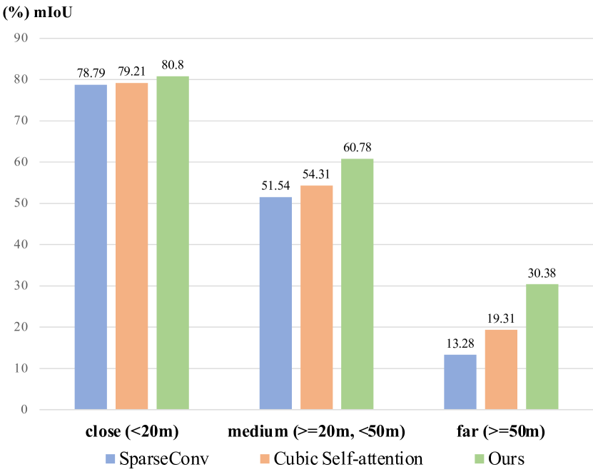
Figure 1: Semantic segmentation performance on nuScenes val set for points at different distances.

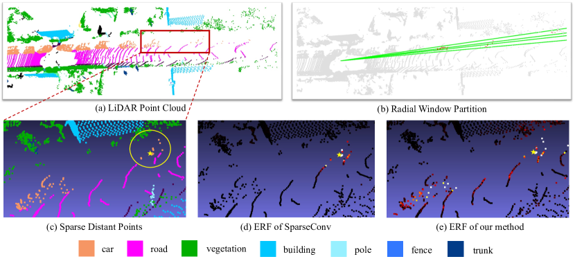
Figure 2: Effective Receptive Field (ERF) of SparseConv and ours. (a) LiDAR point cloud. (b) Radial window partition. Only a single radial window is shown. Points inside the window are marked in red. (c) Zoom-in sparse distant points. A sparse car is circled in yellow. (d) ERF of SparseConv, given the point of interest (with yellow star). White and red denote high contribution. (e) ERF of ours.

We note that the root cause lies in limited receptive field. For sparse distant points, there are few surrounding neighbors. This not only results in inconclusive features, but also hinders enlarging receptive field due to information disconnection. To verify this finding, we visualize the Effective Receptive Field (ERF) [40] of the given feature (shown with the yellow star) in Fig. 2 (d). The ERF cannot be expanded due to disconnection, which is caused by the extreme sparsity of the distant car.

Although window self-attention [30, 22], dilated self-attention [42], and large-kernel CNN [10] have been proposed to conquer the limited receptive field, these methods do not specially deal with LiDAR point distribution, and remain to enlarge receptive field by stacking local operators as before, leaving the information disconnection issue still unsolved. As shown in Fig. 1, the method of cubic self-attention brings a limited improvement.

In this paper, we take a new direction to aggregate long-range information directly in a single operator to suit the varying-sparsity point distribution. We propose the module of SphereFormer to perceive useful information from points 50+ meters away and yield large receptive field for feature extraction. Specifically, we represent the 3D space using spherical coordinates $(r,\theta,\phi)$ with the sensor being the origin, and partition the scene into multiple non-overlapping windows. Unlike the cubic window shape, we design radial windows that are long and narrow. They are obtained by partitioning only along the $\theta$ and $\phi$ axis, as shown in Fig. 2 (b). It is noteworthy that we make it a plugin module to conveniently insert into existing mainstream backbones.

The proposed module does not rely on stacking local operators to expand receptive field, thus avoiding the disconnection issue, as shown in Fig. 2 (e). Also, it facilitates the sparse distant points to aggregate information from the dense-point region, which is often semantically rich. So, the performance of the distant points can be improved significantly (i.e., +17.1% mIoU) as illustrated in Fig. 1.

Moreover, to fit the long and narrow radial windows, we propose exponential splitting to obtain fine-grained relative position encoding. The radius $r$ of a radial window can be over 50 meters, which causes large splitting intervals. It thus results in coarse position encoding when converting relative positions into integer indices. Besides, to let points at varying locations treat local and global information differently, we propose dynamic feature selection to make further improvements.

In total, our contribution is three-fold.

• We propose SphereFormer to directly aggregate long-range information from dense-point region. It increases the receptive field smoothly and helps improve the performance of sparse distant points.

• To accommodate the radial windows, we develop exponential splitting for relative position encoding. Our dynamic feature selection further boosts performance.

• Our method achieves new state-of-the-art results on multiple benchmarks of both semantic segmentation and object detection tasks.

2 Related Work

2.1 LiDAR-based 3D Recognition

Semantic Segmentation.

Segmentation [49, 82, 6, 31, 32, 59, 60, 61, 15, 14, 34] is a fundamental task for vision perception. Approaches for LiDAR-based semantic segmentation can be roughly grouped into three categories, i.e., view-based, point-based, and voxel-based methods. View-based methods either transform the LiDAR point cloud into a range view [67, 68, 3, 43, 46], or use a bird-eye view (BEV) [79] for a 2D network to perform feature extraction. 3D geometric information is simplified.

Point-based methods [44, 45, 58, 72, 28, 56, 30] adopt the point features and positions as inputs, and design abundant operators to aggregate information from neighbors. Moreover, the voxel-based solutions [24, 25, 13] divide the 3D space into regular voxels and then apply sparse convolutions. Further, methods of [70, 55, 88, 12, 37, 29, 17] propose various structures for improved effectiveness. All of them focus on capturing local information. We follow this line of research, and propose to directly aggregate long-range information.

Recently, RPVNet [69] combines the three modalities by feature fusion. Furthermore, 2DPASS [71] incorporates 2D images during training, and [48] fuses multi-modal features. Despite extra 2D information, the performance of these methods still lags behind compared to ours.

Object Detection.

3D object detection frameworks can be roughly categorized into single-stage [75, 84, 26, 83, 36, 11] and two-stage [51, 19, 50, 41] methods. VoxelNet [85] extracts voxel features by PointNet [44] and applies RPN [47] to obtain the proposals. SECOND [73] is efficient thanks to the accelerated sparse convolutions. VoTr [42] applies cubic window attention to voxels. LiDARMultiNet [77] unifies semantic segmentation, panoptic segmentation, and object detection into a single multi-task network with multiple types of supervision. Our experiments are based on CenterPoint [78], which is a widely used anchor-free framework. It is effective and efficient. We aim to enhance the features of sparse distant points, and our proposed module can be conveniently inserted into existing frameworks.

2.2 Vision Transformer

Recently, Transformer [64] become popular in various 2D image understanding tasks [21, 62, 63, 66, 65, 38, 16, 74, 20, 54, 5, 87, 42, 80]. ViT [21] tokenizes every image patch and adopts a Transformer encoder to extract features. Further, PVT [66] presents a hierarchical structure to obtain a feature pyramid for dense prediction. It also proposes Spatial Reduction Attention to save memory. Also, Swin Transformer [38] uses window-based attention and proposes the shifted window operation in the successive Transformer block. Moreover, methods of [16, 74, 20] propose different designs to incorporate long-range dependencies. There are also methods [81, 42, 30, 22, 53] that apply Transformer into 3D vision. Few of them consider the point distribution of LiDAR point cloud. In our work, we utilize the varying-sparsity property, and design radial window self-attention to capture long-range information, especially for the sparse distant points.

3 Our Method

In this section, we first elaborate on radial window partition in Sec. 3.1. Then, we propose the improved position encoding and dynamic feature selection in Sec. 3.2 and 3.3.

3.1 Spherical Transformer

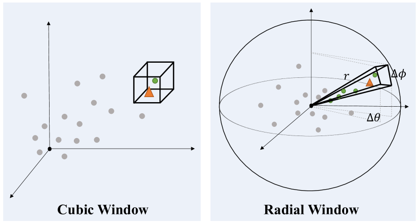
Figure 3: Cubic vs. Radial window partition. The radial window can directly harvest information from the dense-point region, especially for the sparse distant points.

To model the long-range dependency, we adopt the window-attention [38] paradigm. However, unlike the cubic window attention [42, 22, 30], we take advantage of the varying-sparsity property of LiDAR point cloud and present the SphereFormer module, as shown in Fig. 3.

Radial Window Partition.

Specifically, we represent LiDAR point clouds using the spherical coordinate system $(r,\theta,\phi)$ with the LiDAR sensor being the origin. We partition the 3D space along the $\theta$ and $\phi$ axis. We, thus, obtain a number of non-overlapping radial windows with a long and narrow ’pyramid’ shape, as shown in Fig. 3. We obtain the window index for the token at ($r_{i}$, $\theta_{i}$, $\phi_{i}$) as

$$\footnotesize win\_index_{i}=(\lfloor\frac{\theta_{i}}{\Delta\theta}\rfloor,\lfloor\frac{\phi_{i}}{\Delta\phi}\rfloor),$$ (1)

where $\Delta\theta$ and $\Delta\phi$ denote the window size corresponding to the $\theta$ and $\phi$ dimension, respectively.

Tokens with the same window index would be assigned to the same window. The multi-head self-attention [64] is conducted within each window independently as follows.

$$\footnotesize\mathbf{\hat{q}}=\mathbf{f}\cdot\mathbf{W}_{q},\quad\mathbf{\hat{k}}=\mathbf{f}\cdot\mathbf{W}_{k},\quad\mathbf{\hat{v}}=\mathbf{f}\cdot\mathbf{W}_{v},$$ (2)

where $\mathbf{f}\in\mathbb{R}^{n\times c}$ denotes the input features of a window, $\mathbf{W}_{q},\mathbf{W}_{k},\mathbf{W}_{v}\in\mathbb{R}^{c\times c}$ are the linear projection weights, and $\mathbf{\hat{q}},\mathbf{\hat{k}},\mathbf{\hat{v}}\in\mathbb{R}^{n\times c}$ are the projected features. Then, we split the projected features $\mathbf{\hat{q}},\mathbf{\hat{k}},\mathbf{\hat{v}}$ into $h$ heads (i.e., $\mathbb{R}^{n\times(h\times d)}$), and reshape them as $\mathbf{q},\mathbf{k},\mathbf{v}\in\mathbb{R}^{h\times n\times d}$. For each head, we perform dot product and weighted sum as

$$\footnotesize\mathbf{attn}_{k}=\mathbf{softmax}(\mathbf{q}_{k}\cdot\mathbf{k}_{k}^{T}),\vspace{-0.4cm}$$ (3)

$$\footnotesize\hat{\mathbf{z}}_{k}=\mathbf{attn}_{k}\cdot\mathbf{v}_{k},\vspace{0.1cm}$$ (4)

where $\mathbf{q}_{k},\mathbf{k}_{k},\mathbf{v}_{k}\in\mathbb{R}^{n\times d}$ denote the features of the $k$-th head, and $\mathbf{attn}_{k}\in\mathbb{R}^{n\times n}$ is the corresponding attention weight. Finally, we concatenate the features from all heads and apply the final linear projection with weight $\mathbf{W}_{proj}\in\mathbb{R}^{c\times c}$ to yield the output $\mathbf{z}\in\mathbb{R}^{n\times c}$ as

$$\footnotesize\hat{\mathbf{z}}=\mathbf{concat}(\{\hat{\mathbf{z}}_{0},\hat{\mathbf{z}}_{1},...,\hat{\mathbf{z}}_{h-1}\}).\vspace{-0.3cm}$$ (5)

$$\footnotesize\mathbf{z}=\hat{\mathbf{z}}\cdot\mathbf{W}_{proj}.\vspace{0.1cm}$$ (6)

SphereFormer serves as a plugin module and can be conveniently inserted into existing mainstream models, e.g., SparseConvNet [24, 25], MinkowskiNet [13], local window self-attention [42, 30, 22]. In this paper, we find that inserting it into the end of each stage works well, and the network structure is given in the supplementary material. The resulting model can be applied to various downstream tasks, such as semantic segmentation and object detection, with strong performance as produced in experiments.

SphereFormer is effective for the sparse distant points to get long-range information from the dense-point region. Therefore, the sparse distant points overcome the disconnection issue, and increase the effective receptive field.

Comparison with Cylinder3D.

Although both Cylinder3D [88] and ours use polar or spherical coordinates to match LiDAR point distribution, there are two essential differences yet. First, Cylinder3D aims at a more balanced point distribution, while our target is to enlarge the receptive field smoothly and enable the sparse distant points to directly aggregate long-range information from the dense-point region. Second, what Cylinder3D does is replace the cubic voxel shape with the fan-shaped one. It remains to use local neighbors as before and still suffers from limited receptive field for the sparse distant points. Nevertheless, our method changes the way we find neighbors in a single operator (i.e., self-attention) and it is not limited to local neighbors. It thus avoids information separation between near and far objects and connects them in a natural way.

3.2 Position Encoding

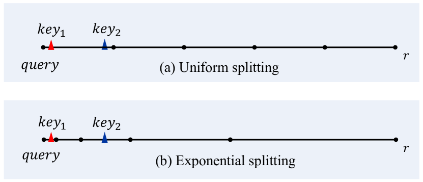
Figure 4: Comparison between (a) uniform splitting and (b) exponential splitting. The $query$ is at the leftmost point.

For the 3D point cloud network, the input features have already incorporated the absolute $xyz$ position. Therefore, there is no need to apply absolute position encoding. Also, we notice that Stratified Transformer [30] develops the contextual relative position encoding. It splits a relative position into several discrete parts uniformly, which converts the continuous relative positions into integers to index the positional embedding tables.

This method works well with local cubic windows. But in our case, the radial window is narrow and long, and its radius $r$ can take even more than 50 meters, which could cause large intervals during discretization and thus coarse-grained positional encoding. As shown in Fig. 4 (a), because of the large interval, $key_{1}$ and $key_{2}$ correspond to the same index. But there is still a considerable distance between them.

Exponential Splitting.

Specifically, since the $r$ dimension covers long distances, we propose exponential splitting for the $r$ dimension as shown in Fig. 4 (b). The splitting interval grows exponentially when the index increases. In this way, the intervals near the $query$ are much smaller, and the $key_{1}$ and $key_{2}$ can be assigned to different position encodings. Meanwhile, we remain to adopt the uniform splitting for the $\theta$ and $\phi$ dimensions. In notation, we have a query token $q_{i}$ and a key token $k_{j}$. Their relative position $(r_{ij},\theta_{ij},\phi_{ij})$ is converted into integer index $(\mathbf{idx}^{r}_{ij},\mathbf{idx}^{\theta}_{ij},\mathbf{idx}^{\phi}_{ij})$ as

$$\mathbf{idx}^{r}_{ij}=\left\{\begin{array}[]{lcl}-\max(0,\lceil\log_{2}(\frac{-r_{ij}}{a})\rceil)-1&&r_{ij}<0\\ 0&&r_{ij}=0\\ \max(0,\lceil\log_{2}(\frac{r_{ij}}{a})\rceil)&&r_{ij}>0\\ \end{array}\right.,$$

$$\mathbf{idx}^{\theta}_{ij}=\lfloor\frac{\theta_{ij}}{\mathbf{inteval}_{\theta}}\rfloor,\quad\mathbf{idx}^{\phi}_{ij}=\lfloor\frac{\phi_{ij}}{\mathbf{inteval}_{\phi}}\rfloor,$$

$$\mathbf{idx}^{x}=\mathbf{idx}^{x}+\frac{L}{2},\quad x\in\{r,\theta,\phi\},$$

where $a$ is a hyper-parameter to control the starting splitting interval, and $L$ is the length of the positional embedding tables. Note that we also add the indices with $\frac{L}{2}$ to make sure they are non-negative.

The above indices ($\mathbf{idx}^{r}_{ij},\mathbf{idx}^{\theta}_{ij},\mathbf{idx}^{\phi}_{ij}$) are then used to index their positional embedding tables $\mathbf{t}_{r},\mathbf{t}_{\theta},\mathbf{t}_{\phi}\in\mathbb{R}^{L\times(h\times d)}$ to find the corresponding position encoding $\mathbf{p}^{r}_{ij},\mathbf{p}^{\theta}_{ij},\mathbf{p}^{\phi}_{ij}\in\mathbb{R}^{h\times d}$, respectively. Then, we sum them up to yield the resultant positional encoding $\mathbf{p}\in\mathbb{R}^{h\times d}$, which then performs dot product with the features of $q_{i}$ and $k_{j}$, respectively. The original Eq. (3) is updated to

$$\mathbf{p} =\mathbf{p}^{r}_{ij}+\mathbf{p}^{\theta}_{ij}+\mathbf{p}^{\phi}_{ij},$$

$$\mathbf{pos\_bias}_{k,i,j} =\mathbf{q}_{k,i}\cdot\mathbf{p}_{k}^{T}+\mathbf{k}_{k,j}\cdot\mathbf{p}_{k}^{T},$$

$$\mathbf{attn}_{k} =\mathbf{softmax}(\mathbf{q}_{k}\cdot\mathbf{k}_{k}^{T}+\mathbf{pos\_bias}_{k}),$$

where $\mathbf{pos\_bias}\in\mathbb{R}^{h\times n\times n}$ is the positional bias to the attention weight, $\mathbf{q}_{k,i}\in\mathbb{R}^{d}$ means the the $k$-th head of the $i$-th query feature, and $\mathbf{p}_{k}\in\mathbb{R}^{d}$ is the $k$-th head of the position encoding $\mathbf{p}$.

The exponential splitting strategy provides smaller splitting intervals for near token pairs and larger intervals for distant ones. This operation enables a fine-grained position representation between near token pairs, and still maintains the same number of intervals in the meanwhile. Even though the splitting intervals become larger for distant token pairs, this solution actually works well since distant token pairs require less fine-grained relative position.

3.3 Dynamic Feature Selection

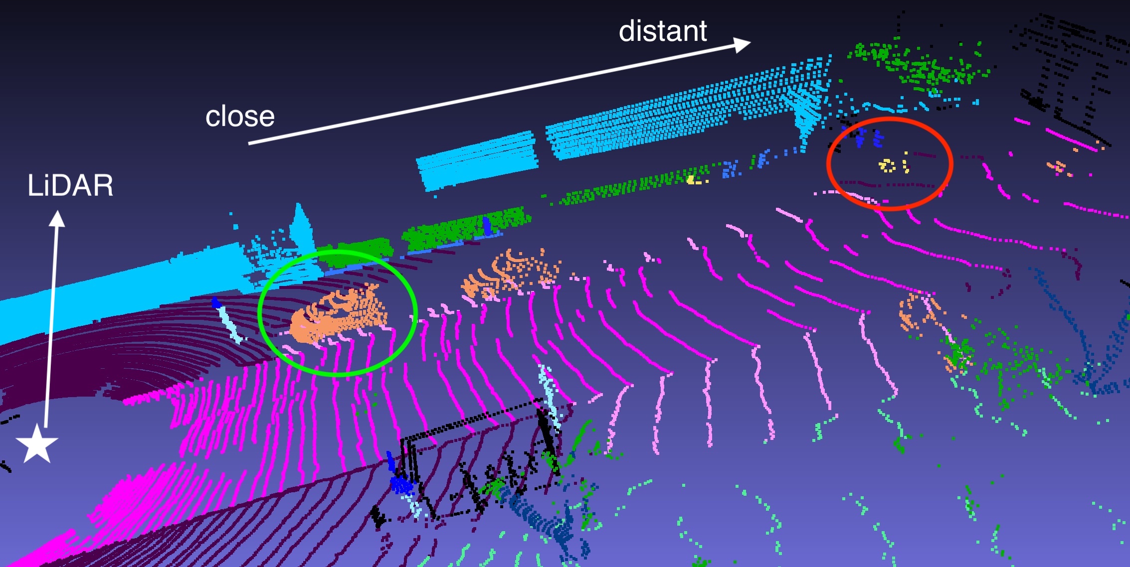
Figure 5: Varying-sparsity property of LiDAR point clouds. The dense close car is marked with a green circle and the sparse distant bicycle is marked with a red circle (best viewed in color).

Point clouds scanned by LiDAR have the varying-sparsity property — close points are dense and distant points are much sparser. This property makes points at different locations perceive different amounts of local information. For example, as shown in Fig. 5, a point of the car (circled in green) near the LiDAR is with rich local geometric information from its dense neighbors, which is already enough for the model to make a correct prediction – incurring more global contexts might be contrarily detrimental. However, a point of bicycle (circled in red) far away from the LiDAR lacks shape information due to the extreme sparsity and even occlusion. Then we should supply long-range contexts as a supplement. This example shows treating all the query points equally is not optimal. We thus propose to dynamically select local or global features to address this issue.

As shown in Fig. 6, for each token, we incorporate not only the radial contextual information, but also local neighbor communication. Specifically, input features are projected into query, key and value features as Eq. (2). Then, the first half of the heads are used for radial window self-attention, and the remaining ones are used for cubic window self-attention. After that, these two features are concatenated and then linearly projected to the final output $\mathbf{z}$ for feature fusion. It enables different points to dynamically select local or global features. Formally, the Equations (3-5) are updated to

$$\mathbf{attn}^{radial}_{k}=\mathbf{softmax}(\mathbf{q}^{radial}_{k}\cdot{\mathbf{k}^{radial}_{k}}^{T}),$$

$$\hat{\mathbf{z}}^{radial}_{k}=\mathbf{attn}^{radial}_{k}\cdot{\mathbf{v}^{radial}_{k}},$$

$$\mathbf{attn}^{cubic}_{k}=\mathbf{softmax}(\mathbf{q}^{cubic}_{k}\cdot{\mathbf{k}^{cubic}_{k}}^{T}),$$

$$\hat{\mathbf{z}}^{cubic}_{k}=\mathbf{attn}^{cubic}_{k}\cdot{\mathbf{v}^{cubic}_{k}},$$

$$\hat{\mathbf{z}}=\mathbf{concat}(\{\hat{\mathbf{z}}^{radial}_{0},\hat{\mathbf{z}}^{radial}_{1},...,\hat{\mathbf{z}}^{radial}_{h/2-1},\hat{z}^{cubic}_{h/2},...,\hat{\mathbf{z}}^{cubic}_{h-1}\}),$$

where $\mathbf{q}^{cubic}_{k},\mathbf{k}^{cubic}_{k},\mathbf{v}^{cubic}_{k}\in\mathbb{R}^{n^{cubic}\times d}$ denote the query, key and value features for the $k$-th head with cubic window partition, and $\mathbf{attn}^{cubic}_{k}\in\mathbb{R}^{n^{cubic}\times n^{cubic}}$ denotes the cubic window attention weight for the $k$-th head.

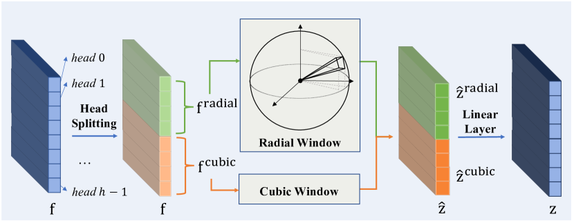
Figure 6: Dynamic feature selection. We split the heads to conduct radial and cubic window self-attention respectively.

4 Experiments

In this section, we first introduce the experimental setting in Sec. 4.1. Then, we show the semantic segmentation and object detection results in Sec. 4.2 and 4.3. The ablation study and visual comparison are shown in Sec. 4.4 and 4.5. Our code and models will be made publicly available.

4.1 Experimental Setting

Network Architecture.

For semantic segmentation, we adopt the encoder-decoder structure and follow U-Net [49] to concatenate the fine-grained encoder features in the decoder. We follow [88] to use SparseConv [24, 25] as our baseline model. There are a total of 5 stages whose channel numbers are $[32,64,128,256,256]$, and there are two residual blocks at each stage. Our proposed module is stacked at the end of each encoding stage. For object detection, we adopt CenterPoint [78] as our baseline model, where the backbone possesses 4 stages whose channel numbers are $[16,32,64,128]$. Our proposed module is stacked at the end of the second and third stages. Note that our proposed module incurs negligible extra parameters, and more details are given in the supplementary material.

Datasets.

Following previous work, we evaluate methods on nuScenes [4], SemanticKITTI [3], and Waymo Open Dataset [52] (WOD) for semantic segmentation. For object detection, we evaluate our methods on the nuScenes [4] dataset. The details of the datasets are given in the supplementary material.

Method	mIoU	road	sidewalk	parking	other-gro.	building	car	truck	bicycle	motorcycle	other-veh.	vegetation	trunk	terrain	person	bicyclist	motorcyclist	fence	pole	traffic sign
SqueezeSegV2 [67]	39.7	88.6	67.6	45.8	17.7	73.7	81.8	13.4	18.5	17.9	14.0	71.8	35.8	60.2	20.1	25.1	3.9	41.1	20.2	26.3
DarkNet53Seg [3]	49.9	91.8	74.6	64.8	27.9	84.1	86.4	25.5	24.5	32.7	22.6	78.3	50.1	64.0	36.2	33.6	4.7	55.0	38.9	52.2
RangeNet53++ [43]	52.2	91.8	75.2	65.0	27.8	87.4	91.4	25.7	25.7	34.4	23.0	80.5	55.1	64.6	38.3	38.8	4.8	58.6	47.9	55.9
3D-MiniNet [1]	55.8	91.6	74.5	64.2	25.4	89.4	90.5	28.5	42.3	42.1	29.4	82.8	60.8	66.7	47.8	44.1	14.5	60.8	48.0	56.6
SqueezeSegV3 [68]	55.9	91.7	74.8	63.4	26.4	89.0	92.5	29.6	38.7	36.5	33.0	82.0	58.7	65.4	45.6	46.2	20.1	59.4	49.6	58.9
PointNet++ [45]	20.1	72.0	41.8	18.7	5.6	62.3	53.7	0.9	1.9	0.2	0.2	46.5	13.8	30.0	0.9	1.0	0.0	16.9	6.0	8.9
TangentConv [56]	40.9	83.9	63.9	33.4	15.4	83.4	90.8	15.2	2.7	16.5	12.1	79.5	49.3	58.1	23.0	28.4	8.1	49.0	35.8	28.5
PointASNL [72]	46.8	87.4	74.3	24.3	1.8	83.1	87.9	39.0	0.0	25.1	29.2	84.1	52.2	70.6	34.2	57.6	0.0	43.9	57.8	36.9
RandLA-Net [28]	55.9	90.5	74.0	61.8	24.5	89.7	94.2	43.9	29.8	32.2	39.1	83.8	63.6	68.6	48.4	47.4	9.4	60.4	51.0	50.7
KPConv [58]	58.8	90.3	72.7	61.3	31.5	90.5	95.0	33.4	30.2	42.5	44.3	84.8	69.2	69.1	61.5	61.6	11.8	64.2	56.4	47.4
PolarNet [79]	54.3	90.8	74.4	61.7	21.7	90.0	93.8	22.9	40.3	30.1	28.5	84.0	65.5	67.8	43.2	40.2	5.6	61.3	51.8	57.5
JS3C-Net [70]	66.0	88.9	72.1	61.9	31.9	92.5	95.8	54.3	59.3	52.9	46.0	84.5	69.8	67.9	69.5	65.4	39.9	70.8	60.7	68.7
SPVNAS [55]	67.0	90.2	75.4	67.6	21.8	91.6	97.2	56.6	50.6	50.4	58.0	86.1	73.4	71.0	67.4	67.1	50.3	66.9	64.3	67.3
Cylinder3D [88]	68.9	92.2	77.0	65.0	32.3	90.7	97.1	50.8	67.6	63.8	58.5	85.6	72.5	69.8	73.7	69.2	48.0	66.5	62.4	66.2
RPVNet [69]	70.3	93.4	80.7	70.3	33.3	93.5	97.6	44.2	68.4	68.7	61.1	86.5	75.1	71.7	75.9	74.4	43.4	72.1	64.8	61.4
(AF)2-S3Net [12]	70.8	92.0	76.2	66.8	45.8	92.5	94.3	40.2	63.0	81.4	40.0	78.6	68.0	63.1	76.4	81.7	77.7	69.6	64.0	73.3
PVKD [27]	71.2	91.8	70.9	77.5	41.0	92.4	97.0	67.9	69.3	53.5	60.2	86.5	73.8	71.9	75.1	73.5	50.5	69.4	64.9	65.8
2DPASS [71]	72.9	89.7	74.7	67.4	40.0	93.5	97.0	61.1	63.6	63.4	61.5	86.2	73.9	71.0	77.9	81.3	74.1	72.9	65.0	70.4
Ours	74.8	91.8	78.2	69.7	41.3	93.8	97.5	59.6	70.1	70.5	67.7	86.7	75.1	72.4	79.0	80.4	75.3	72.8	66.8	72.9

Table 1: Semantic segmentation results on SemanticKITTI test set. Methods published before the submission deadline (11/11/2022) are listed.

Method	Input	mIoU	FW mIoU	barrier	bicycle	bus	car	construction	motorcycle	pedestrian	traffic cone	trailer	truck	driveable	other flat	sidewalk	terrain	manmade	vegetation
PolarNet [79]	L	69.4	87.4	72.2	16.8	77.0	86.5	51.1	69.7	64.8	54.1	69.7	63.5	96.6	67.1	77.7	72.1	87.1	84.5
JS3C-Net [70]	L	73.6	88.1	80.1	26.2	87.8	84.5	55.2	72.6	71.3	66.3	76.8	71.2	96.8	64.5	76.9	74.1	87.5	86.1
Cylinder3D [88]	L	77.2	89.9	82.8	29.8	84.3	89.4	63.0	79.3	77.2	73.4	84.6	69.1	97.7	70.2	80.3	75.5	90.4	87.6
AMVNet [35]	L	77.3	90.1	80.6	32.0	81.7	88.9	67.1	84.3	76.1	73.5	84.9	67.3	97.5	67.4	79.4	75.5	91.5	88.7
SPVCNN [55]	L	77.4	89.7	80.0	30.0	91.9	90.8	64.7	79.0	75.6	70.9	81.0	74.6	97.4	69.2	80.0	76.1	89.3	87.1
(AF)2-S3Net [12]	L	78.3	88.5	78.9	52.2	89.9	84.2	77.4	74.3	77.3	72.0	83.9	73.8	97.1	66.5	77.5	74.0	87.7	86.8
PMF [89]	L+C	77.0	89.0	82.0	40.0	81.0	88.0	64.0	79.0	80.0	76.0	81.0	67.0	97.0	68.0	78.0	74.0	90.0	88.0
2D3DNet [23]	L+C	80.0	90.1	83.0	59.4	88.0	85.1	63.7	84.4	82.0	76.0	84.8	71.9	96.9	67.4	79.8	76.0	92.1	89.2
2DPASS [71]	L	80.8	90.1	81.7	55.3	92.0	91.8	73.3	86.5	78.5	72.5	84.7	75.5	97.6	69.1	79.9	75.5	90.2	88.0
Ours	L	81.9	91.7	83.3	39.2	94.7	92.5	77.5	84.2	84.4	79.1	88.4	78.3	97.9	69.0	81.5	77.2	93.4	90.2

Table 2: Semantic segmentation results on nuScenes test set. Methods published before the submission deadline (11/11/2022) are listed.

Implementation Details.

For semantic segmentation, we use 4 GeForce RTX 3090 GPUs for training. We train the models for 50 epochs with AdamW [39] optimizer and ‘poly’ scheduler where power is set to 0.9. The learning rate and weight decay are set to $0.006$ and $0.01$, respectively. Batch size is set to 16 on nuScenes, and 8 on both SemanticKITTI and Waymo Open Dataset. The window size is set to $[120m,2^{\circ},2^{\circ}]$ for $(r,\theta,\phi)$ on both nuScenes and SemanticKITTI, and $[80m,1.5^{\circ},1.5^{\circ}]$ on Waymo Open Dataset. During data preprocessing, we confine the input scene to the range from $[-51.2m,-51.2m,-4m]$ to $[51.2m,51.2m,2.4m]$ on SemanticKITTI and $[-75.2m,-75.2m,-2m]$ to $[75.2m,75.2m,4m]$ on Waymo. Also, we set the voxel size to $0.1m$ on both nuScenes and Waymo, and $0.05m$ on SemanticKITTI.

For object detection, we adopt the OpenPCDet [57] codebase and follow the default CenterPoint [78] to set the training hyper-parameters. We set the window size to $[120m,1.5^{\circ},1.5^{\circ}]$.

4.2 Semantic Segmentation Results

Method	mIoU	barrier	bicycle	bus	car	construction	motorcycle	pedestrian	traffic cone	trailer	truck	driveable	other flat	sidewalk	terrain	manmade	vegetation
RangeNet53++ [43]	65.5	66.0	21.3	77.2	80.9	30.2	66.8	69.6	52.1	54.2	72.3	94.1	66.6	63.5	70.1	83.1	79.8
PolarNet [79]	71.0	74.7	28.2	85.3	90.9	35.1	77.5	71.3	58.8	57.4	76.1	96.5	71.1	74.7	74.0	87.3	85.7
Salsanext [18]	72.2	74.8	34.1	85.9	88.4	42.2	72.4	72.2	63.1	61.3	76.5	96.0	70.8	71.2	71.5	86.7	84.4
AMVNet [35]	76.1	79.8	32.4	82.2	86.4	62.5	81.9	75.3	72.3	83.5	65.1	97.4	67.0	78.8	74.6	90.8	87.9
Cylinder3D [88]	76.1	76.4	40.3	91.2	93.8	51.3	78.0	78.9	64.9	62.1	84.4	96.8	71.6	76.4	75.4	90.5	87.4
PVKD [27]	76.0	76.2	40.0	90.2	94.0	50.9	77.4	78.8	64.7	62.0	84.1	96.6	71.4	76.4	76.3	90.3	86.9
RPVNet [69]	77.6	78.2	43.4	92.7	93.2	49.0	85.7	80.5	66.0	66.9	84.0	96.9	73.5	75.9	76.0	90.6	88.9
Ours	78.4	77.7	43.8	94.5	93.1	52.4	86.9	81.2	65.4	73.4	85.3	97.0	73.4	75.4	75.0	91.0	89.2
Ours‡	79.5	78.7	46.7	95.2	93.7	54.0	88.9	81.1	68.0	74.2	86.2	97.2	74.3	76.3	75.8	91.4	89.7

Table 3: Semantic segmentation results on nuScenes val set. $\;\;{}^{\ddagger}$ denotes using rotation and translation testing-time augmentations.

Method	mIoU	close	med.	far	car	truck	bus	other-veh.	motorcyclist	bicyclist	pedestrian	sign	traffic-light	pole	con.cone	bicycle	motorcycle	building	vegetation	tree-trunk	curb	road	lane-marker	other-gro.	walkable	sidewalk
SparseConv [25]	66.6	67.8	64.1	52.6	94.4	59.8	85.1	37.8	2.2	69.1	89.3	73.4	40.4	74.8	57.3	66.6	75.2	95.5	91.3	67.0	68.1	92.3	41.7	30.1	79.0	75.6
Ours	69.9	70.3	68.6	61.9	94.5	61.6	87.7	40.2	0.9	69.7	90.2	73.9	41.8	77.2	65.4	71.9	83.7	95.9	91.7	68.4	69.8	93.3	53.9	47.9	80.8	77.2

Table 4: Semantic segmentation results on Waymo Open Dataset val set.

The results on SemanticKITTI test set are shown in Table 1. Our method yields $74.8\%$ mIoU, a new state-of-the-art result. Compared to the methods based on range images [67, 43] and Bird-Eye-View (BEV) [79], ours gives a result with over $20\%$ mIoU performance gain. Moreover, thanks to the capability of directly aggregating long-range information, our method significantly outperforms the models based on sparse convolution [70, 88, 55, 12, 69]. It is also notable that our method outperforms 2DPASS [71] that uses extra 2D images in training by $1.9\%$ mIoU.

In Tables 2 and 3, we also show the semantic segmentation results on nuScenes test and val set, respectively. Our method consistently outperforms others by a large margin, and achieves the 1^st place on the benchmark. It is intriguing to note that our method is purely based on LiDAR data, and it works even better than approaches of [89, 23, 71] that use additional 2D information.

Moreover, we demonstrate the semantic segmentation results on Waymo Open Dataset val set in Table 4. Our model outperforms the baseline model with a substantial gap of $3.3\%$ mIoU. Also, it is worth noting that our method achieves a $9.3\%$ mIoU performance gain for the far points, i.e., the sparse distant points.

4.3 Object Detection Results

ID	RadialWin	ExpSplit	Dynamic	close	medium	far	overall	$\Delta$
I				78.79	51.54	13.28	75.21	0.00
II	✓			78.95	57.21	26.67	76.31	+1.10
III	✓	✓		79.92	61.09	31.10	77.60	+2.39
IV	✓		✓	79.51	58.94	28.95	77.05	+1.84
V	✓	✓	✓	80.80	60.78	30.38	78.41	+3.20

Table 5: Ablation study. RadialWin: Radial window shape. ExpSplit: Exponential splitting. Dynamic: Dynamic Feature Selection. Metric: mIoU.

Method	close	medium	far	overall
Cubic	79.21	54.31	19.31	76.19
Radial	80.80	60.78	30.38	78.41

Table 6: Comparison between radial and cubic window shapes.

window size	$1.0^{\circ}$	$1.5^{\circ}$	$2.0^{\circ}$	$2.5^{\circ}$
mIoU (%)	77.8	77.5	78.4	77.6

Table 7: Effect of window size for the $\theta$ and $\phi$ dimensions.

Method	NDS	mAP	Car	Truck	Bus	Trailer	C.V.	Ped.	Mot.	Byc.	T.C.	Bar.
PointPillars [33]	45.3	30.5	68.4	23.0	28.2	23.4	4.1	59.7	27.4	1.1	30.8	38.9
3DSSD [76]	56.4	42.6	81.2	47.2	61.4	30.5	12.6	70.2	36.0	8.6	31.1	47.9
CBSG [86]	63.3	52.8	81.1	48.5	54.9	42.9	10.5	80.1	51.5	22.3	70.9	65.7
CenterPoint [78]	65.5	58.0	84.6	51.0	60.2	53.2	17.5	83.4	53.7	28.7	76.7	70.9
HotSpotNet [8]	66.0	59.3	83.1	50.9	56.4	53.3	23.0	81.3	63.5	36.6	73.0	71.6
CVCNET [7]	66.6	58.2	82.6	49.5	59.4	51.1	16.2	83.0	61.8	38.8	69.7	69.7
TransFusion [2]	70.2	65.5	86.2	56.7	66.3	58.8	28.2	86.1	68.3	44.2	82.0	78.2
Focals Conv [9]	70.0	63.8	86.7	56.3	67.7	59.5	23.8	87.5	64.5	36.3	81.4	74.1
Ours	70.7	65.5	84.9	55.1	66.4	59.3	29.9	86.0	71.4	47.1	79.7	75.2
Ours‡	72.8	68.5	85.3	57.9	67.0	59.9	33.7	88.6	76.3	56.4	82.2	78.2

• $\;\;{}^{\ddagger}$ Flipping and rotation testing-time augmentations.

Table 8: Object detection results on nuScenes test set. Methods published before the submission deadline (11/11/2022) are listed.

Our method also achieves strong performance in object detection. As shown in Table 8, our method outperforms other published methods on nuScenes test set, and ranks 3^rd on the LiDAR-only benchmark. It shows that directly aggregating long-range information is also beneficial for object detection. It also manifests the capability of our method to generalize to instance-level tasks.

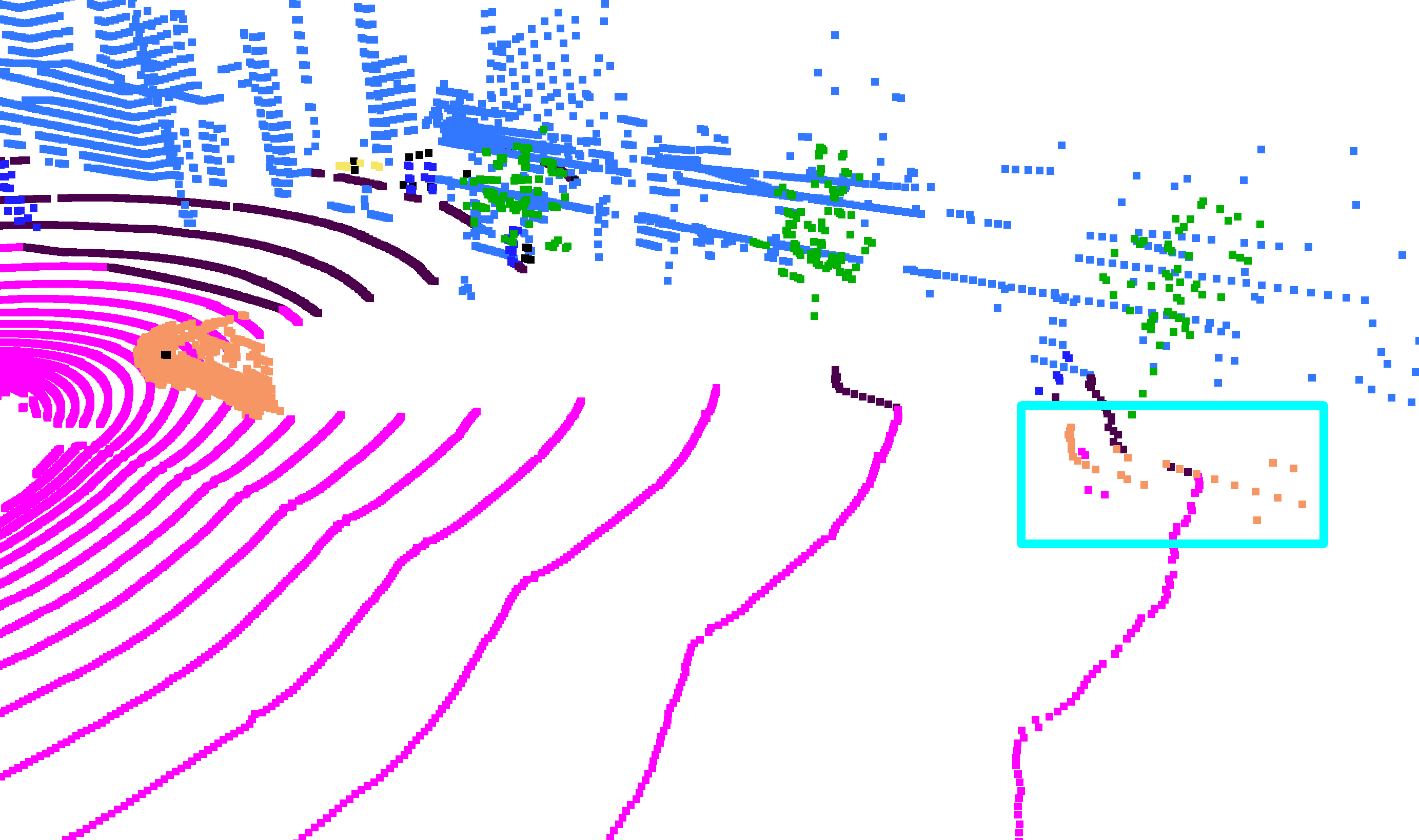
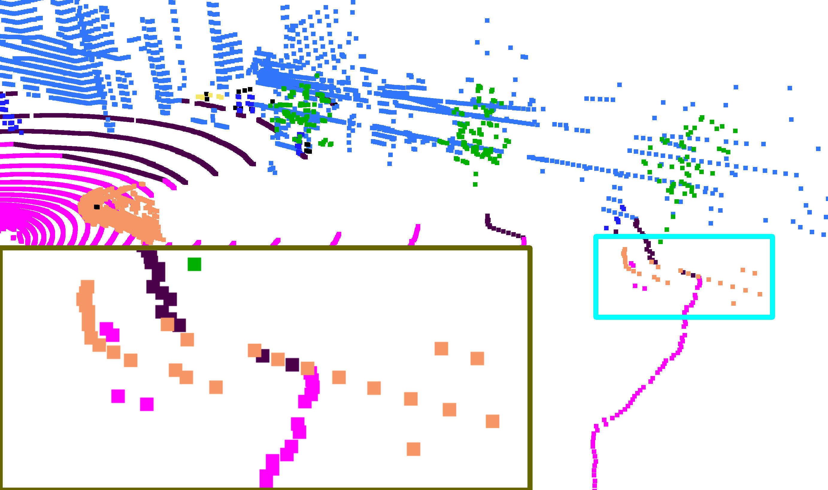
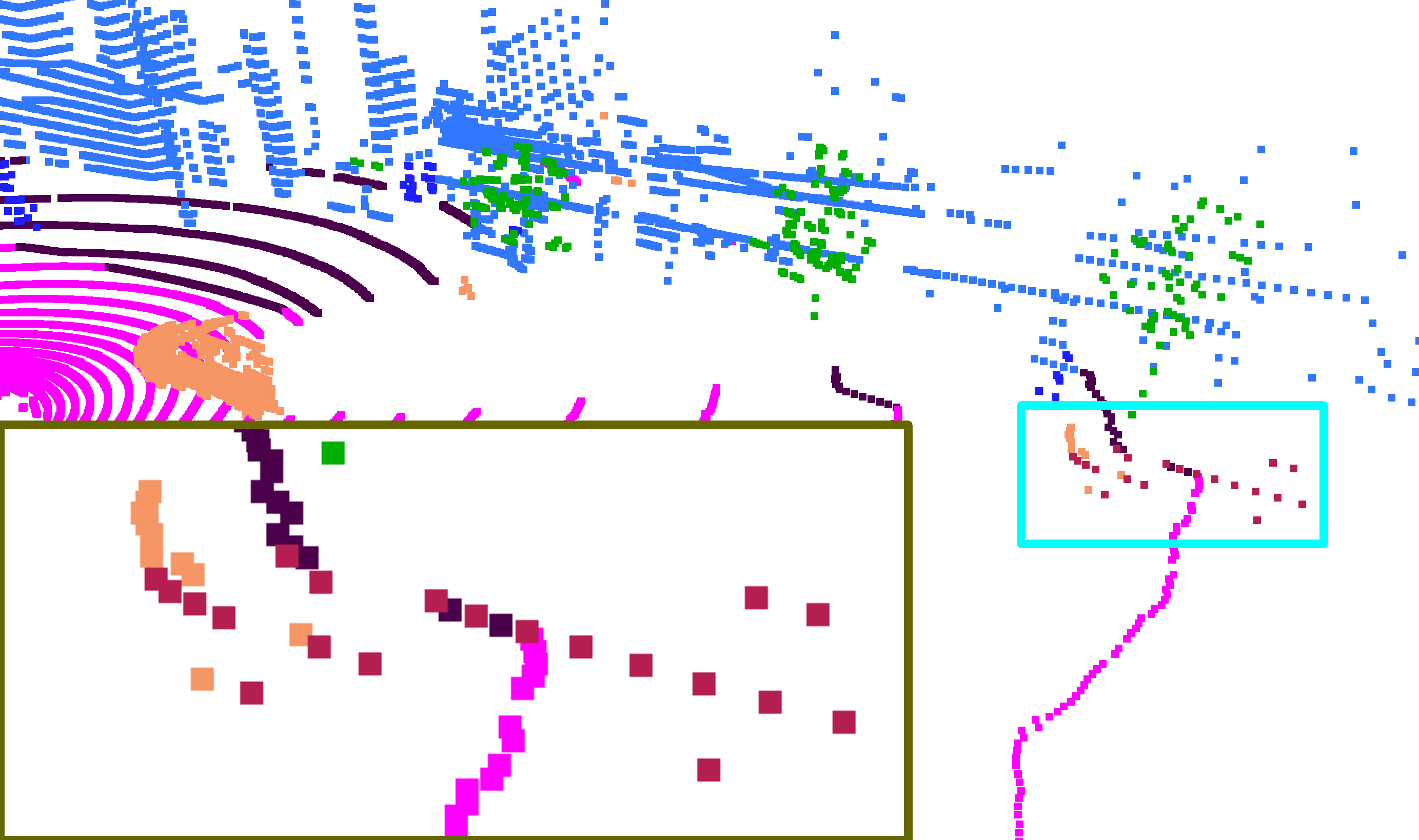
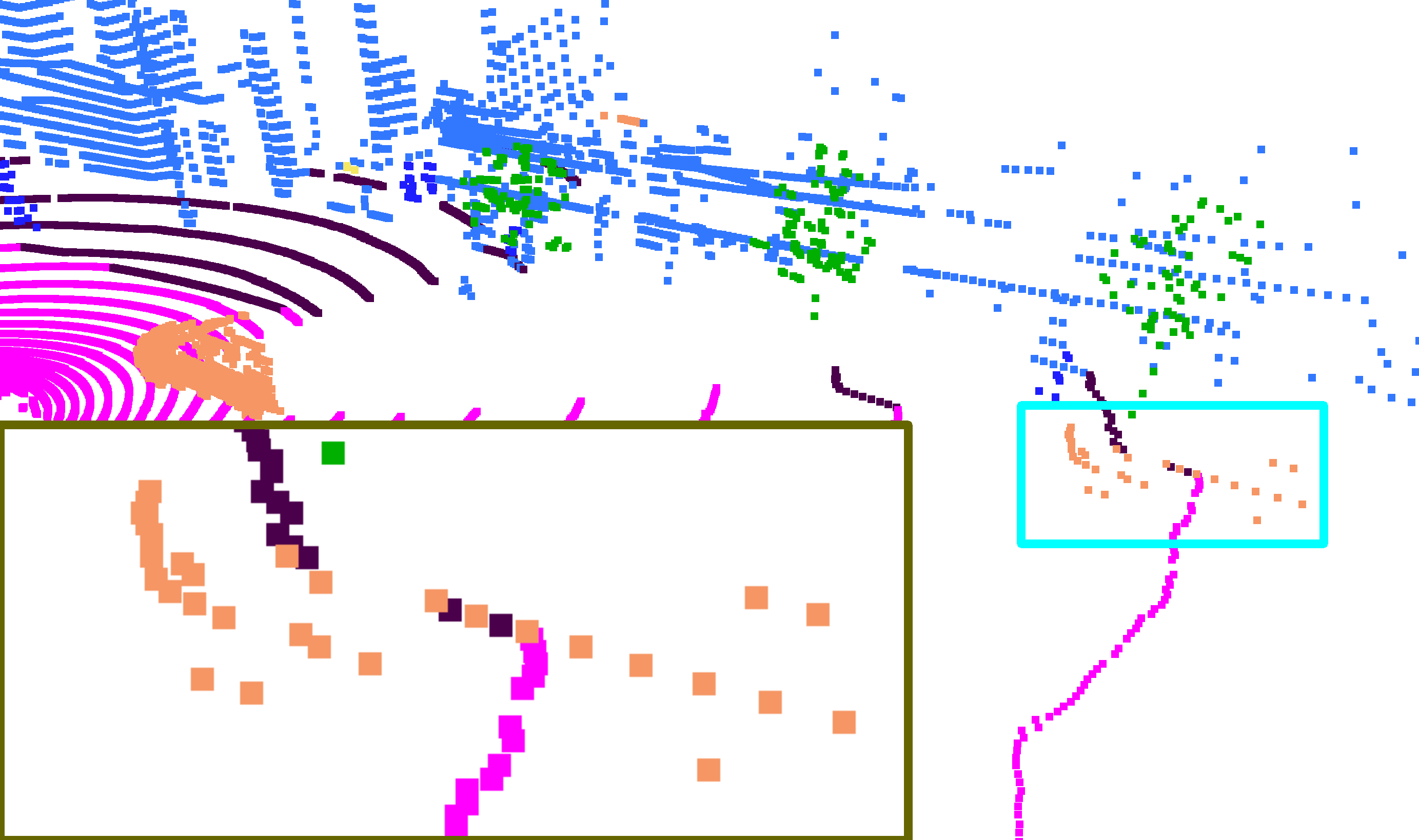
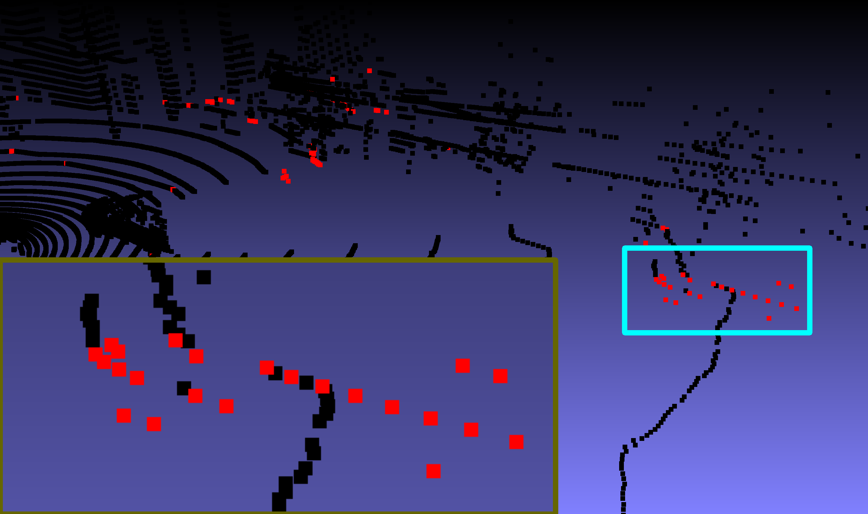
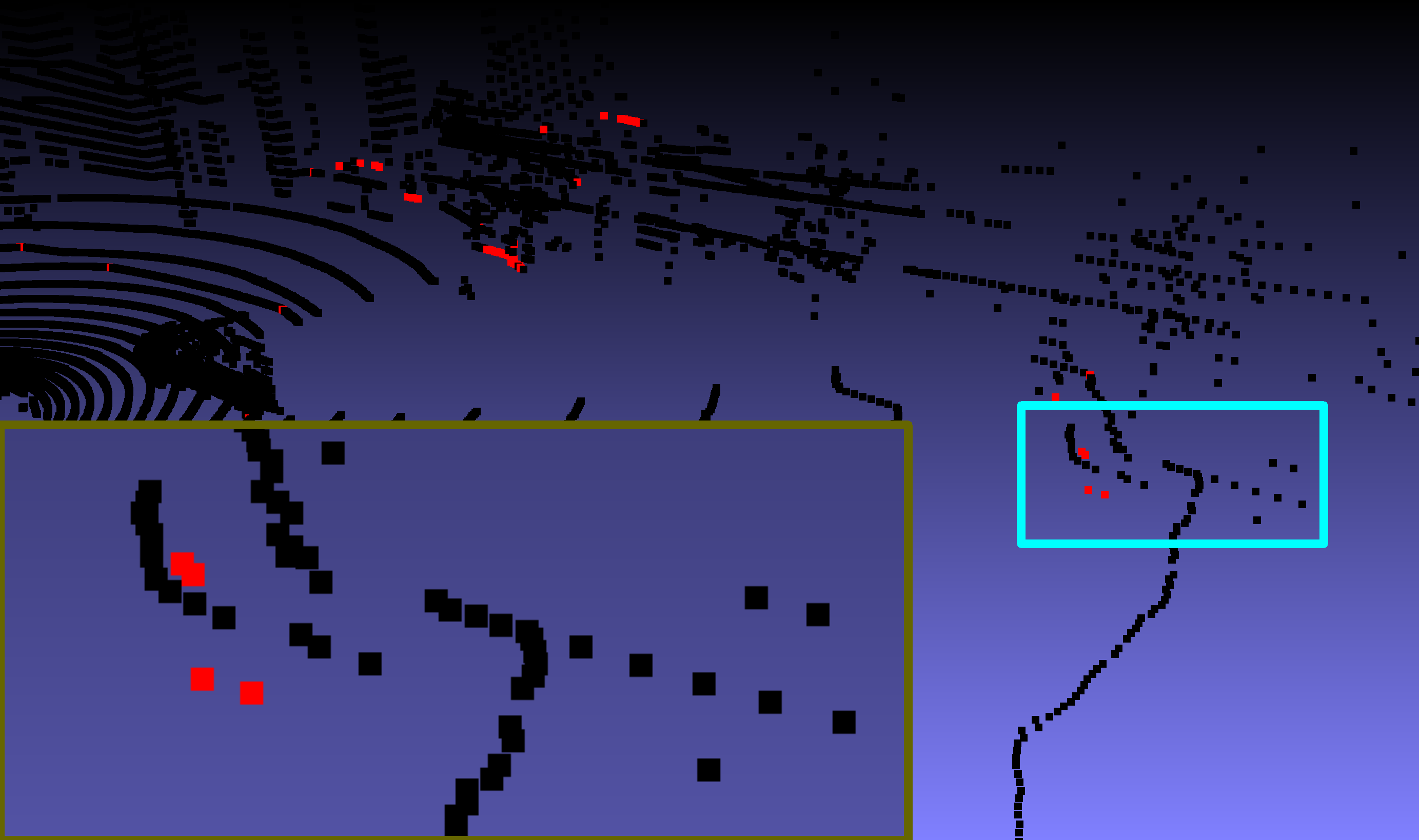
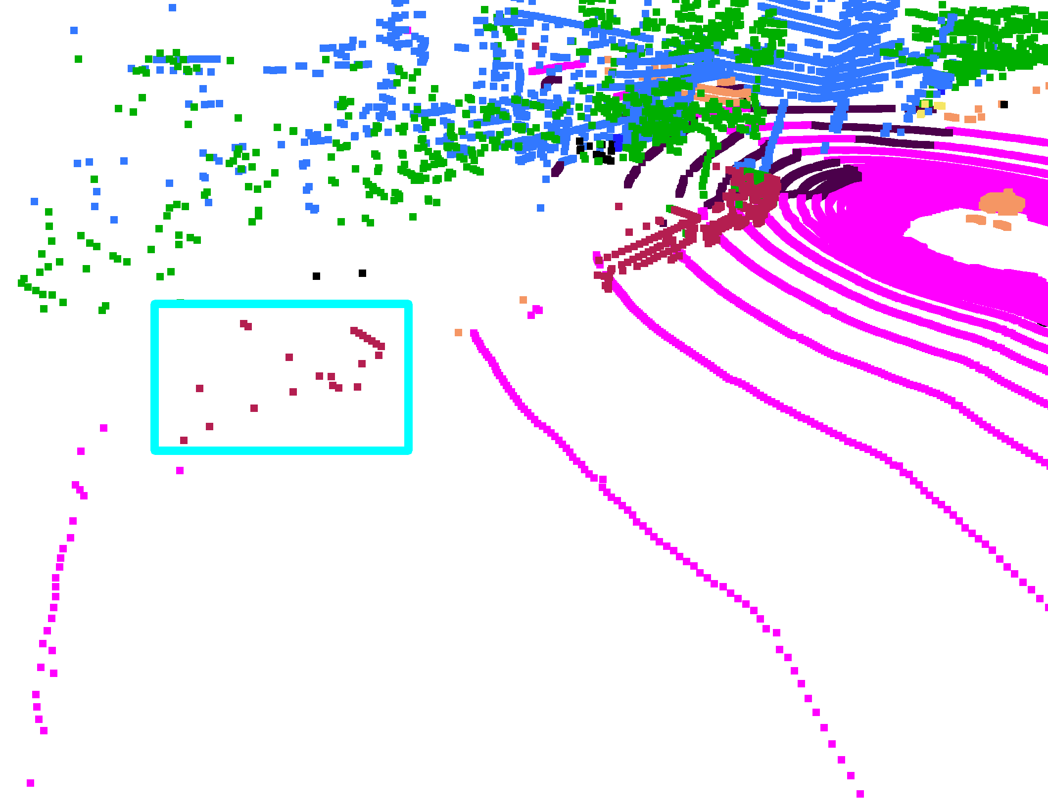
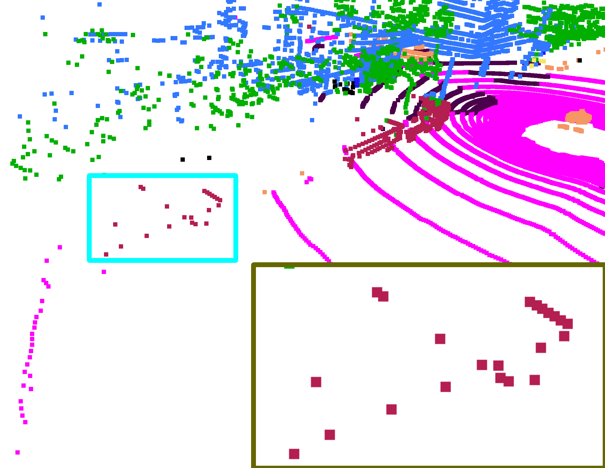
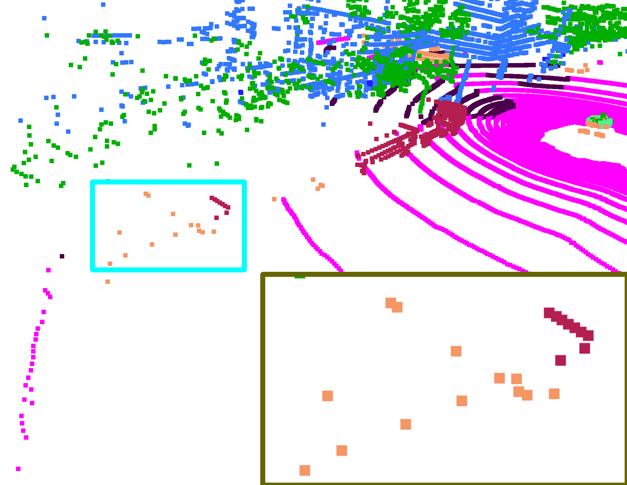
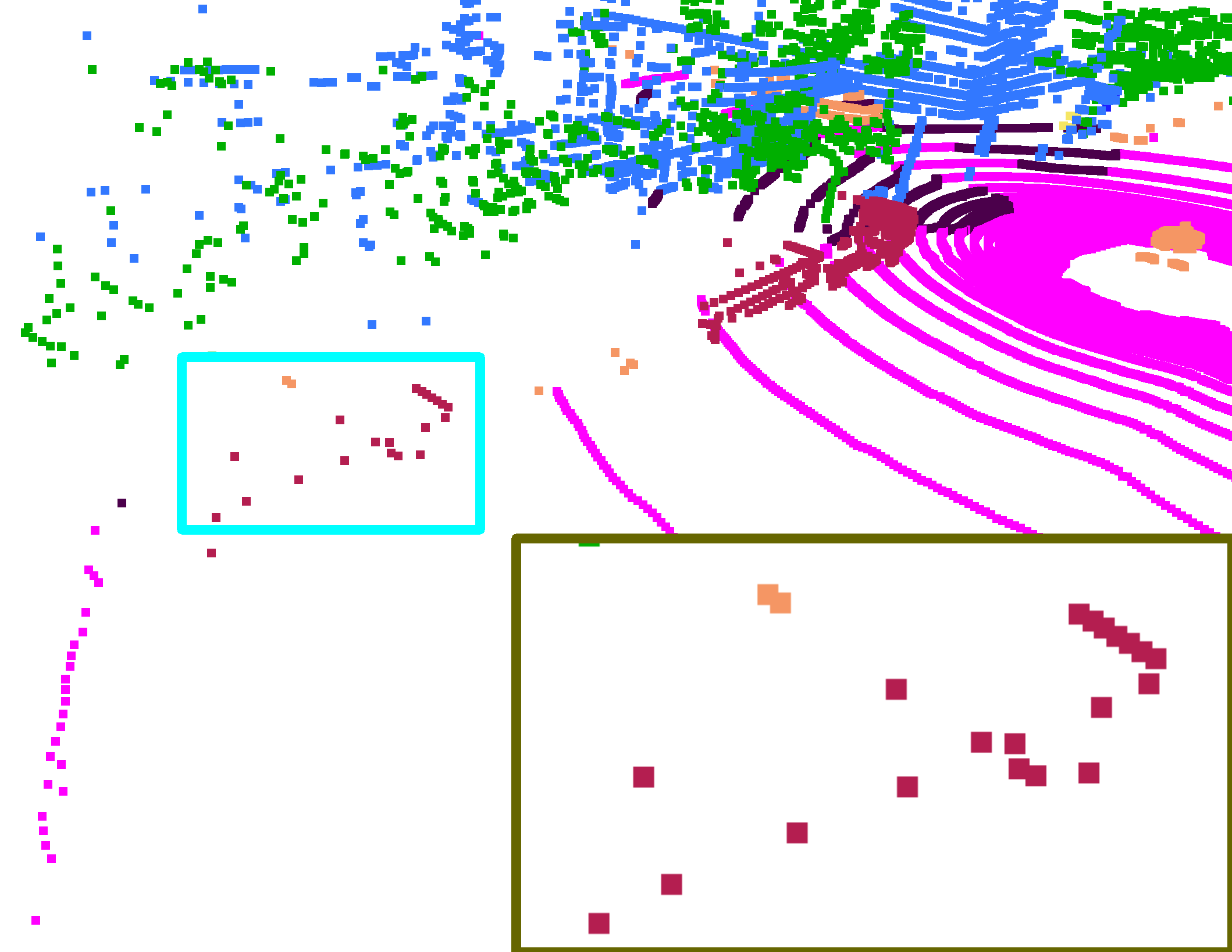
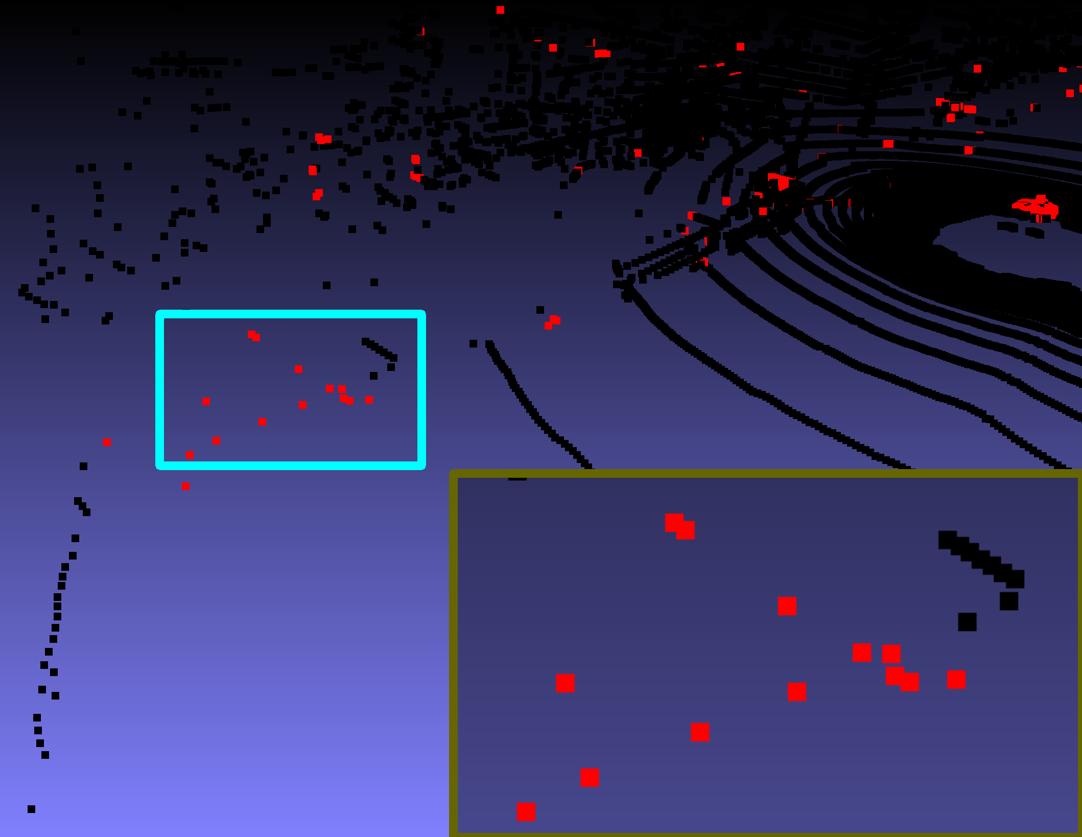
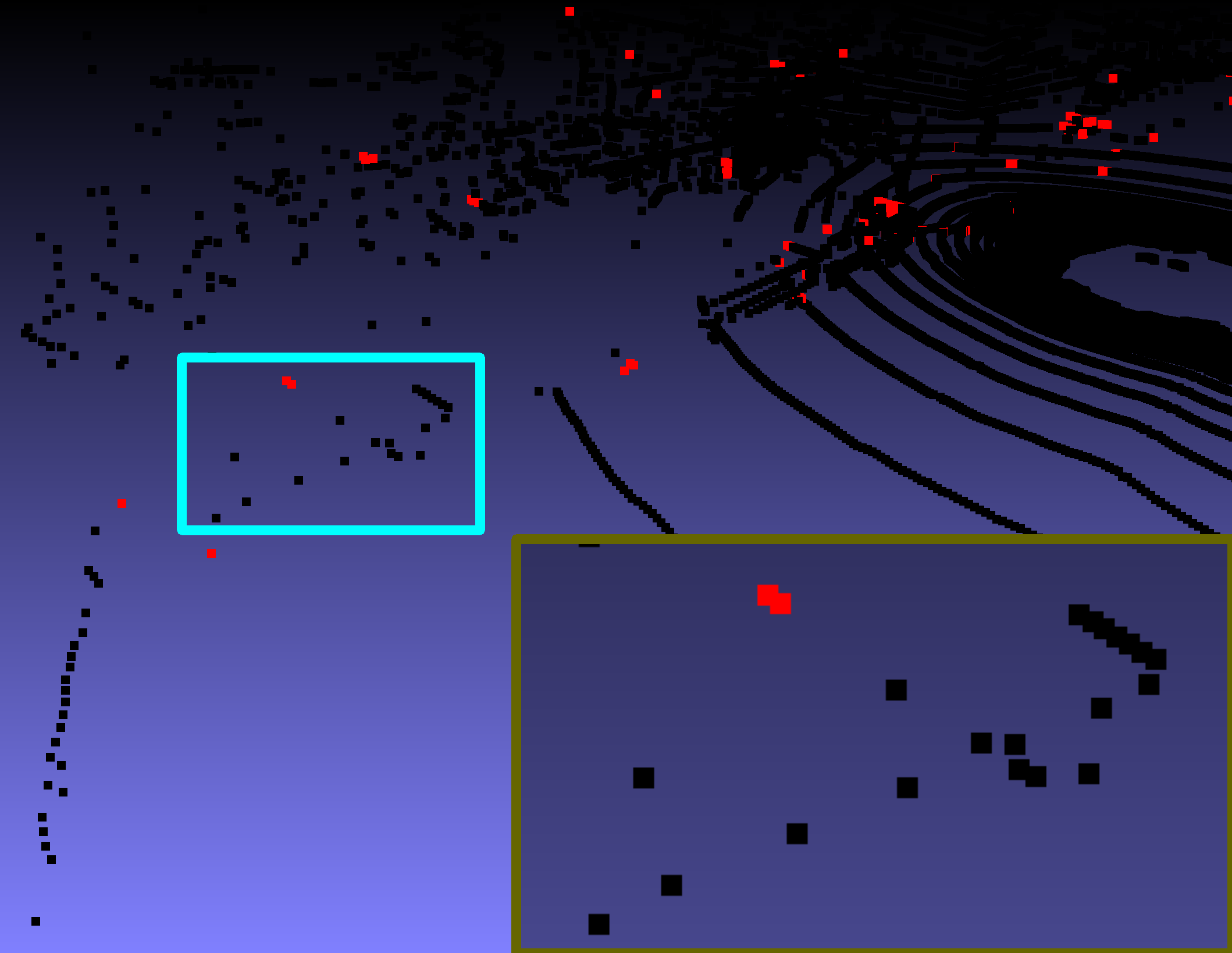
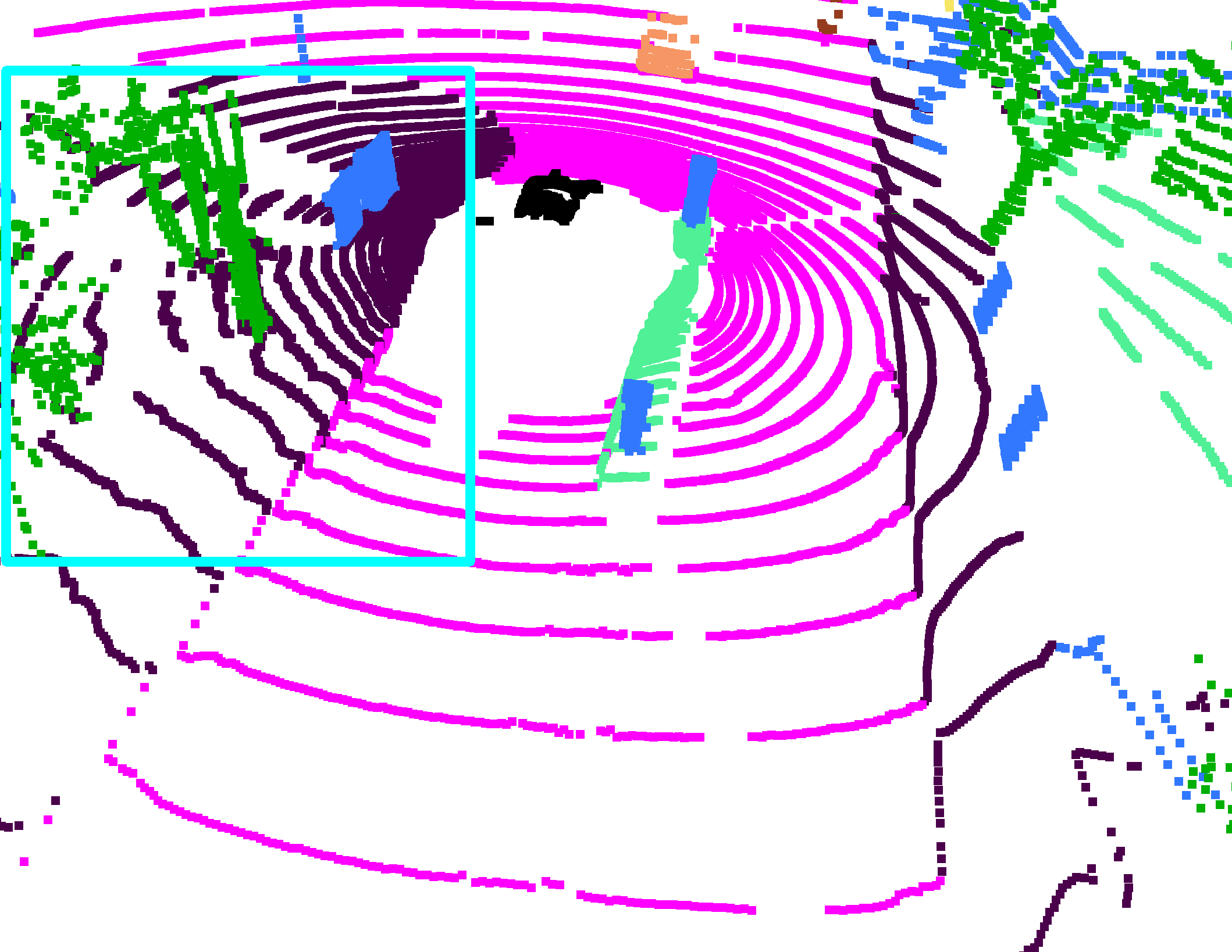
Input

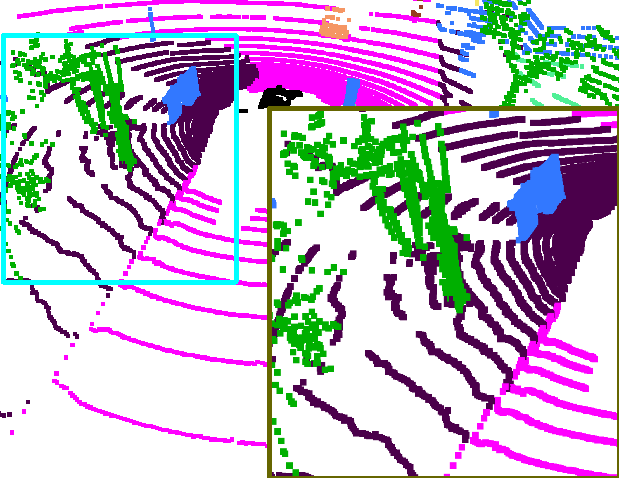
Ground Truth

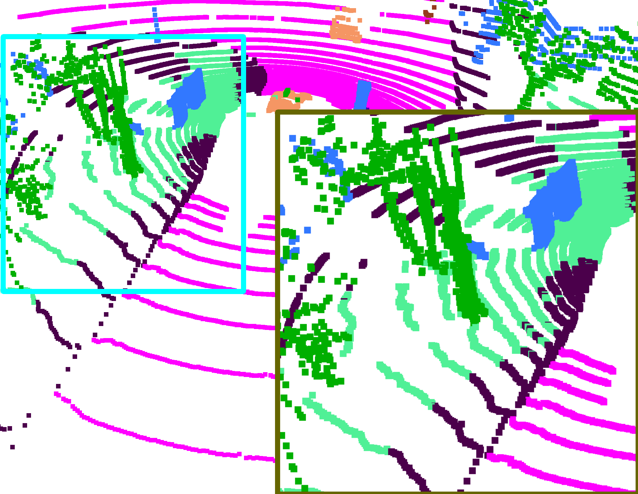
SparseConv

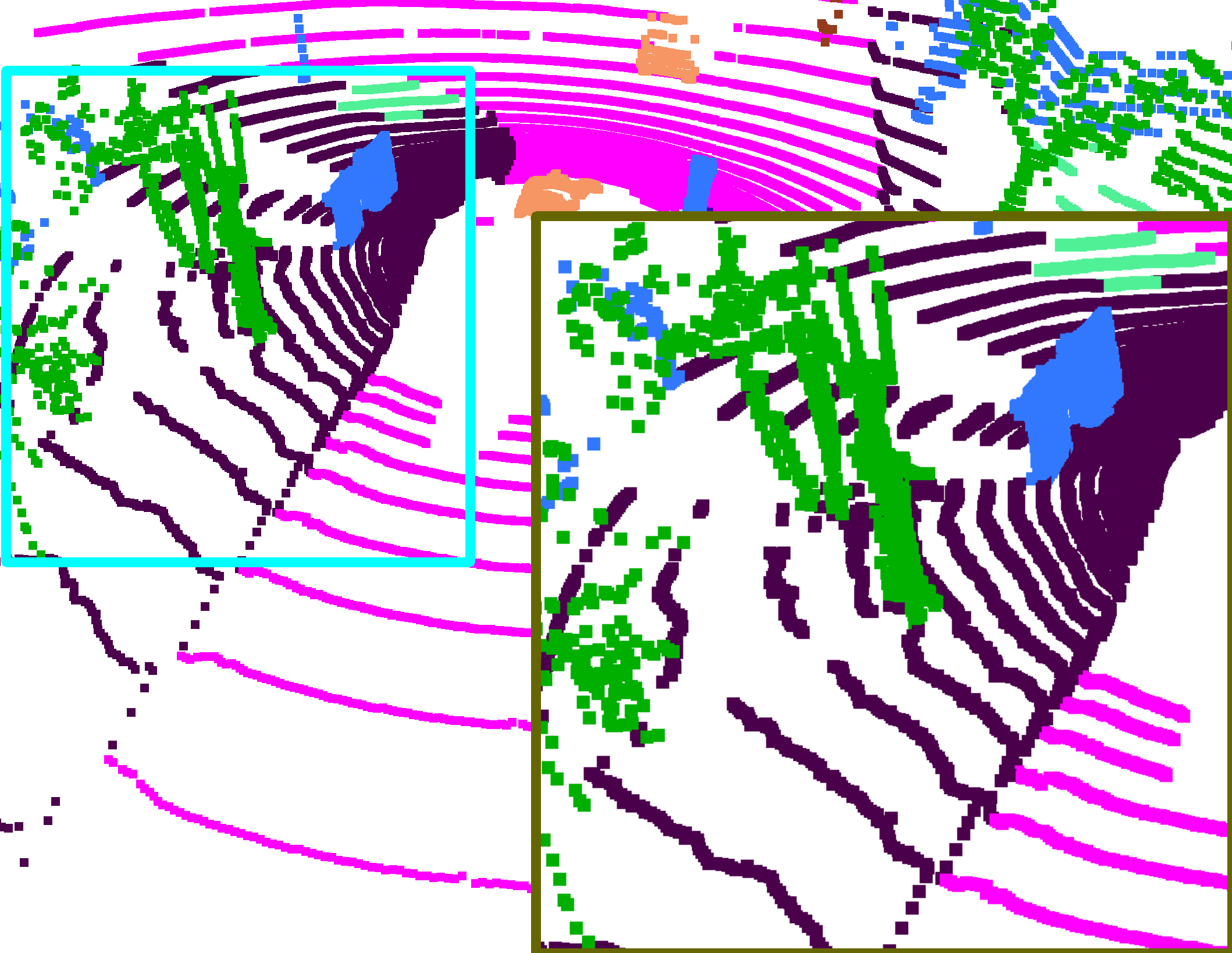
Ours

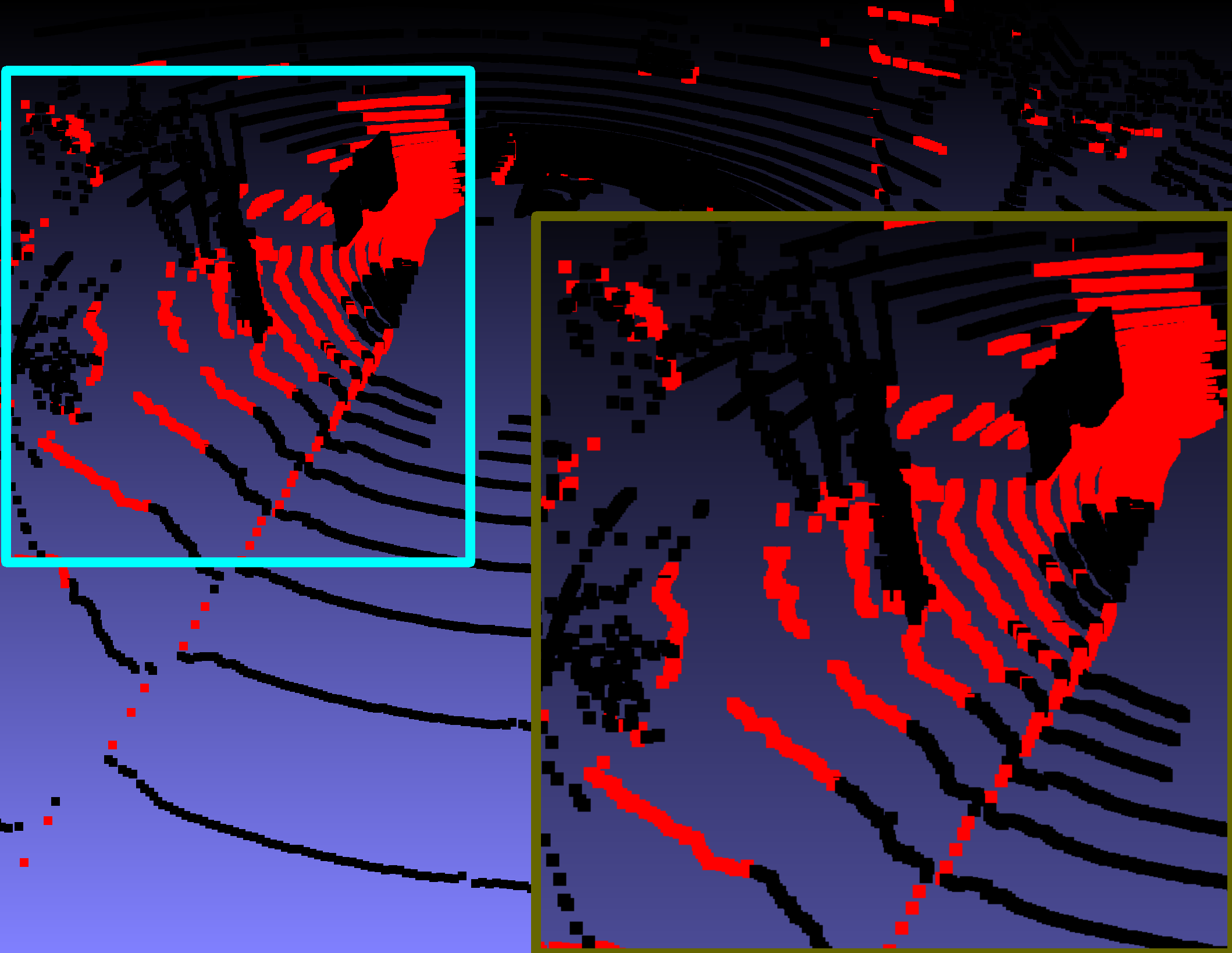
SparseConv

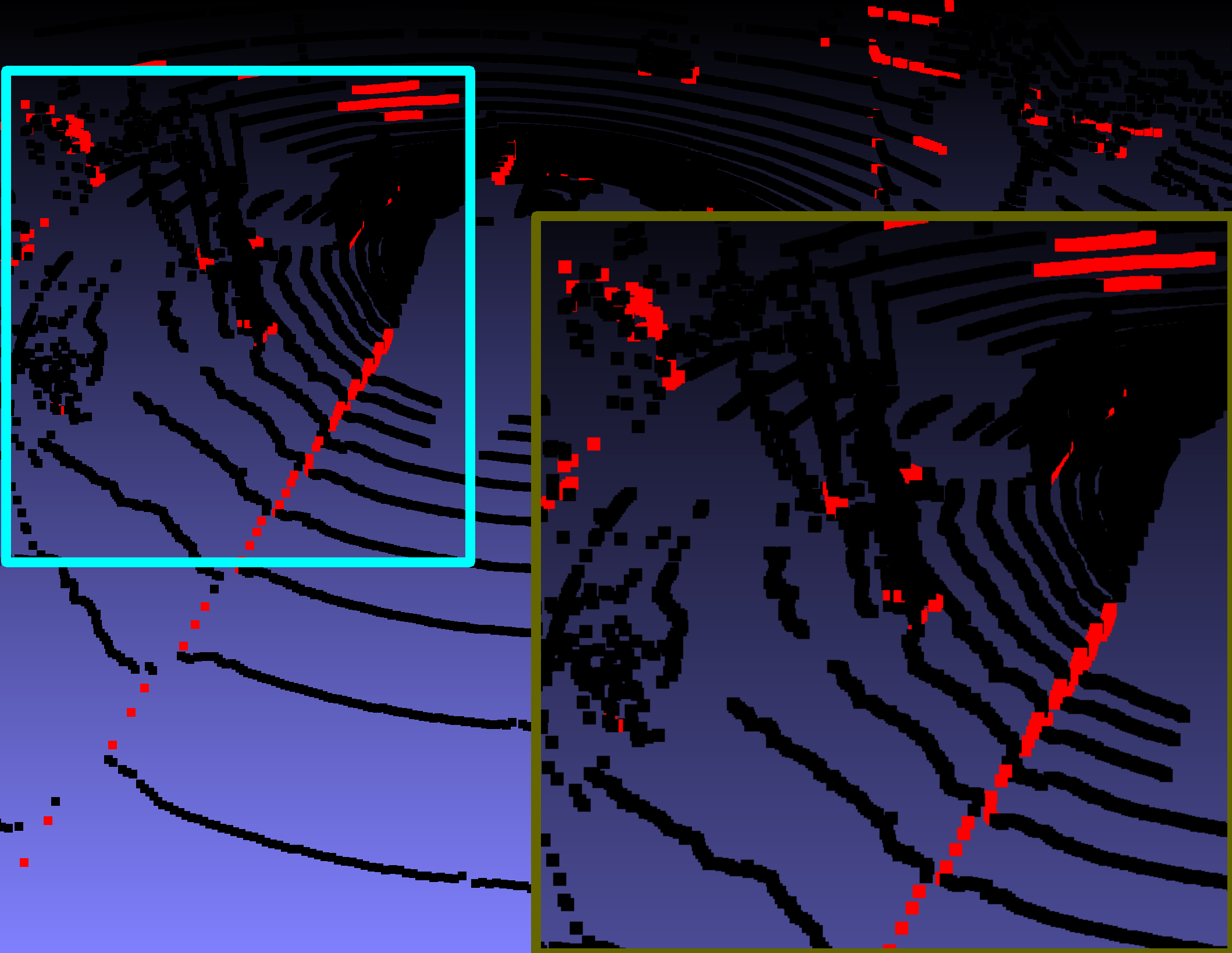
Ours

barrier bicycle truck car driveable surface manmade terrain sidewalk vegetation

Figure 7: Visual comparison between vanilla SparseConv and ours (best viewed in color and by zoom-in). The brown box is the zoom-in of the cyan box. The last two columns are the difference maps with the ground truth. More examples are given in the supplementary material.

4.4 Ablation Study

To testify the effectiveness of each component, we conduct an extensive ablation study and list the result in Table 5. The Experiment I (Exp. I for short) is our baseline model of SparseConv. Unless otherwise specified, we train the models on nuScenes train set and make evaluations on nuScenes val set for the ablation study. To comprehensively reveal the effect, we also report the performance at different distances, i.e., close ($\leq 20m$), medium ($>20m$ & $\leq 50m$), far ($>50m$) distances.

Window Shape.

By comparing Experiments I and II in Table 5, we can conclude that the radial window shape is beneficial. Further, the improvement stems mainly from better handling the medium and far points, where we yield $5.67\%$ and $13.39\%$ mIoU performance gain, respectively. This result exactly verifies the benefit of aggregating long-range information with the radial window shape.

Moreover, we also compare the radial window shape with the cubic one proposed in [22, 42, 30]. As shown in Table 6, the radial window shape considerably outperforms the cubic one.

Besides, we investigate the effect of window size as shown in Table 7. Setting it too small may make it hard to capture meaningful information, while setting it too large may increase the optimization difficulty.

Exponential Splitting.

Compared to Exp. IV, Exp. V improves with $1.36\%$ more mIoU, which shows the effectiveness. Moreover, the consistent conclusion could be drawn from Experiments II and III, where we witness $3.88\%$ and $4.43\%$ more mIoU for the medium and far points, respectively. Also, we notice that with exponential splitting, all the close, medium, and far points are better dealt with.

Dynamic Feature Selection.

From the comparison between Experiments III and V, we note that dynamic feature selection brings a $0.8\%$ mIoU performance gain. Interestingly, we further notice that the gain mainly comes from the close points, which indicates that the close points may not rely too much on global information, since the dense local information is already enough for correct predictions for the dense close points. It also reveals the fact that points at varying locations should be treated differently. Moreover, the comparison between Exp. II and IV leads to consistent conclusion. Although the performance of medium and far decreases a little, the overall mIoU still increases, since their points number is much than that of the close points.

4.5 Visual Comparison

As shown in Fig. 7, we visually compare the baseline model (i.e., SparseConv) and ours. It visually indicates that with our proposed module, more sparse distant objects are recognized, which are highlighted with cyan boxes. More examples are given in the supplementary material.

5 Conclusion

We have studied and dealt with varying-sparsity LiDAR point distribution. We proposed SphereFormer to enable the sparse distant points to directly aggregate information from the close ones. We designed radial window self-attention, which enlarges the receptive field for distant points to intervene with close dense ones. Also, we presented exponential splitting to yield more detailed position encoding. Dynamically selecting local or global features is also helpful. Our method demonstrates powerful performance, ranking 1^st on both nuScenes and SemanticKITTI semantic segmentation benchmarks and achieving the 3^rd on nuScenes object detection benchmark. It shows a new way to further enhance 3D visual understanding. Our limitations are discussed in the supplementary material.

References

- [1] Inigo Alonso, Luis Riazuelo, Luis Montesano, and Ana C Murillo. 3d-mininet: Learning a 2d representation from point clouds for fast and efficient 3d lidar semantic segmentation. IEEE Robotics and Automation Letters, 2020.
- [2] Xuyang Bai, Zeyu Hu, Xinge Zhu, Qingqiu Huang, Yilun Chen, Hongbo Fu, and Chiew-Lan Tai. Transfusion: Robust lidar-camera fusion for 3d object detection with transformers. In CVPR, 2022.
- [3] Jens Behley, Martin Garbade, Andres Milioto, Jan Quenzel, Sven Behnke, Cyrill Stachniss, and Jurgen Gall. Semantickitti: A dataset for semantic scene understanding of lidar sequences. In ICCV, 2019.
- [4] Holger Caesar, Varun Bankiti, Alex H Lang, Sourabh Vora, Venice Erin Liong, Qiang Xu, Anush Krishnan, Yu Pan, Giancarlo Baldan, and Oscar Beijbom. nuscenes: A multimodal dataset for autonomous driving. In CVPR, 2020.
- [5] Nicolas Carion, Francisco Massa, Gabriel Synnaeve, Nicolas Usunier, Alexander Kirillov, and Sergey Zagoruyko. End-to-end object detection with transformers. In ECCV, 2020.
- [6] Liang-Chieh Chen, Yukun Zhu, George Papandreou, Florian Schroff, and Hartwig Adam. Encoder-decoder with atrous separable convolution for semantic image segmentation. In ECCV, 2018.
- [7] Qi Chen, Lin Sun, Ernest Cheung, and Alan L Yuille. Every view counts: Cross-view consistency in 3d object detection with hybrid-cylindrical-spherical voxelization. NeurIPS, 2020.
- [8] Qi Chen, Lin Sun, Zhixin Wang, Kui Jia, and Alan Yuille. Object as hotspots: An anchor-free 3d object detection approach via firing of hotspots. In ECCV, 2020.
- [9] Yukang Chen, Yanwei Li, Xiangyu Zhang, Jian Sun, and Jiaya Jia. Focal sparse convolutional networks for 3d object detection. In CVPR, 2022.
- [10] Yukang Chen, Jianhui Liu, Xiaojuan Qi, Xiangyu Zhang, Jian Sun, and Jiaya Jia. Scaling up kernels in 3d cnns. arXiv:2206.10555, 2022.
- [11] Yukang Chen, Jianhui Liu, Xiangyu Zhang, Xiaojuan Qi, and Jiaya Jia. Fully sparse voxelnet for 3d object detection and tracking. In CVPR, 2023.
- [12] Ran Cheng, Ryan Razani, Ehsan Taghavi, Enxu Li, and Bingbing Liu. 2-s3net: Attentive feature fusion with adaptive feature selection for sparse semantic segmentation network. In CVPR, 2021.
- [13] Christopher Choy, JunYoung Gwak, and Silvio Savarese. 4d spatio-temporal convnets: Minkowski convolutional neural networks. In CVPR, 2019.
- [14] Ruihang Chu, Yukang Chen, Tao Kong, Lu Qi, and Lei Li. Icm-3d: Instantiated category modeling for 3d instance segmentation. IEEE RAL, 7(1):57–64, 2021.
- [15] Ruihang Chu, Xiaoqing Ye, Zhengzhe Liu, Xiao Tan, Xiaojuan Qi, Chi-Wing Fu, and Jiaya Jia. Twist: Two-way inter-label self-training for semi-supervised 3d instance segmentation. In CVPR, 2022.
- [16] Xiangxiang Chu, Zhi Tian, Yuqing Wang, Bo Zhang, Haibing Ren, Xiaolin Wei, Huaxia Xia, and Chunhua Shen. Twins: Revisiting the design of spatial attention in vision transformers. arXiv:2104.13840, 2021.
- [17] Taco S Cohen, Mario Geiger, Jonas Köhler, and Max Welling. Spherical cnns. arXiv preprint arXiv:1801.10130, 2018.
- [18] Tiago Cortinhal, George Tzelepis, and Eren Erdal Aksoy. Salsanext: Fast, uncertainty-aware semantic segmentation of lidar point clouds. In International Symposium on Visual Computing, 2020.
- [19] Jiajun Deng, Shaoshuai Shi, Peiwei Li, Wengang Zhou, Yanyong Zhang, and Houqiang Li. Voxel R-CNN: towards high performance voxel-based 3d object detection. In AAAI, 2021.
- [20] Xiaoyi Dong, Jianmin Bao, Dongdong Chen, Weiming Zhang, Nenghai Yu, Lu Yuan, Dong Chen, and Baining Guo. Cswin transformer: A general vision transformer backbone with cross-shaped windows. arXiv:2107.00652, 2021.
- [21] Alexey Dosovitskiy, Lucas Beyer, Alexander Kolesnikov, Dirk Weissenborn, Xiaohua Zhai, Thomas Unterthiner, Mostafa Dehghani, Matthias Minderer, Georg Heigold, Sylvain Gelly, Jakob Uszkoreit, and Neil Houlsby. An image is worth 16x16 words: Transformers for image recognition at scale. ICLR, 2021.
- [22] Lue Fan, Ziqi Pang, Tianyuan Zhang, Yu-Xiong Wang, Hang Zhao, Feng Wang, Naiyan Wang, and Zhaoxiang Zhang. Embracing Single Stride 3D Object Detector with Sparse Transformer. In CVPR, 2022.
- [23] Kyle Genova, Xiaoqi Yin, Abhijit Kundu, Caroline Pantofaru, Forrester Cole, Avneesh Sud, Brian Brewington, Brian Shucker, and Thomas Funkhouser. Learning 3d semantic segmentation with only 2d image supervision. In 3DV, 2021.
- [24] Benjamin Graham, Martin Engelcke, and Laurens van der Maaten. 3d semantic segmentation with submanifold sparse convolutional networks. In CVPR, 2018.
- [25] Benjamin Graham and Laurens van der Maaten. Submanifold sparse convolutional networks. arXiv:1706.01307, 2017.
- [26] Chenhang He, Hui Zeng, Jianqiang Huang, Xian-Sheng Hua, and Lei Zhang. Structure aware single-stage 3d object detection from point cloud. In CVPR, pages 11870–11879, 2020.
- [27] Yuenan Hou, Xinge Zhu, Yuexin Ma, Chen Change Loy, and Yikang Li. Point-to-voxel knowledge distillation for lidar semantic segmentation. In CVPR, 2022.
- [28] Qingyong Hu, Bo Yang, Linhai Xie, Stefano Rosa, Yulan Guo, Zhihua Wang, Niki Trigoni, and Andrew Markham. Randla-net: Efficient semantic segmentation of large-scale point clouds. In CVPR, 2020.
- [29] Li Jiang, Shaoshuai Shi, Zhuotao Tian, Xin Lai, Shu Liu, Chi-Wing Fu, and Jiaya Jia. Guided point contrastive learning for semi-supervised point cloud semantic segmentation. In ICCV, 2021.
- [30] Xin Lai, Jianhui Liu, Li Jiang, Liwei Wang, Hengshuang Zhao, Shu Liu, Xiaojuan Qi, and Jiaya Jia. Stratified transformer for 3d point cloud segmentation. In CVPR, 2022.
- [31] Xin Lai, Zhuotao Tian, Li Jiang, Shu Liu, Hengshuang Zhao, Liwei Wang, and Jiaya Jia. Semi-supervised semantic segmentation with directional context-aware consistency. In CVPR, 2021.
- [32] Xin Lai, Zhuotao Tian, Xiaogang Xu, Yingcong Chen, Shu Liu, Hengshuang Zhao, Liwei Wang, and Jiaya Jia. Decouplenet: Decoupled network for domain adaptive semantic segmentation. In ECCV, 2022.
- [33] Alex H Lang, Sourabh Vora, Holger Caesar, Lubing Zhou, Jiong Yang, and Oscar Beijbom. Pointpillars: Fast encoders for object detection from point clouds. In CVPR, 2019.
- [34] Yiming Li, Tao Kong, Ruihang Chu, Yifeng Li, Peng Wang, and Lei Li. Simultaneous semantic and collision learning for 6-dof grasp pose estimation. In IROS. IEEE, 2021.
- [35] Venice Erin Liong, Thi Ngoc Tho Nguyen, Sergi Widjaja, Dhananjai Sharma, and Zhuang Jie Chong. Amvnet: Assertion-based multi-view fusion network for lidar semantic segmentation. arXiv:2012.04934, 2020.
- [36] Jianhui Liu, Yukang Chen, Xiaoqing Ye, Zhuotao Tian, Xiao Tan, and Xiaojuan Qi. Spatial pruned sparse convolution for efficient 3d object detection. In NeurIPS, 2022.
- [37] Minghua Liu, Yin Zhou, Charles R Qi, Boqing Gong, Hao Su, and Dragomir Anguelov. Less: Label-efficient semantic segmentation for lidar point clouds. In ECCV, 2022.
- [38] Ze Liu, Yutong Lin, Yue Cao, Han Hu, Yixuan Wei, Zheng Zhang, Stephen Lin, and Baining Guo. Swin transformer: Hierarchical vision transformer using shifted windows. ICCV, 2021.
- [39] Ilya Loshchilov and Frank Hutter. Decoupled weight decay regularization. arXiv:1711.05101, 2017.
- [40] Wenjie Luo, Yujia Li, Raquel Urtasun, and Richard Zemel. Understanding the effective receptive field in deep convolutional neural networks. In NeurIPS, 2016.
- [41] Jiageng Mao, Minzhe Niu, Haoyue Bai, Xiaodan Liang, Hang Xu, and Chunjing Xu. Pyramid R-CNN: towards better performance and adaptability for 3d object detection. In ICCV, 2021.
- [42] Jiageng Mao, Yujing Xue, Minzhe Niu, Haoyue Bai, Jiashi Feng, Xiaodan Liang, Hang Xu, and Chunjing Xu. Voxel transformer for 3d object detection. In ICCV, 2021.
- [43] Andres Milioto, Ignacio Vizzo, Jens Behley, and Cyrill Stachniss. Rangenet++: Fast and accurate lidar semantic segmentation. In 2019 IEEE/RSJ international conference on intelligent robots and systems (IROS), 2019.
- [44] Charles R Qi, Hao Su, Kaichun Mo, and Leonidas J Guibas. Pointnet: Deep learning on point sets for 3d classification and segmentation. In CVPR, 2017.
- [45] Charles Ruizhongtai Qi, Li Yi, Hao Su, and Leonidas J Guibas. Pointnet++: Deep hierarchical feature learning on point sets in a metric space. NeurIPS, 2017.
- [46] Ryan Razani, Ran Cheng, Ehsan Taghavi, and Liu Bingbing. Lite-hdseg: Lidar semantic segmentation using lite harmonic dense convolutions. In ICRA, 2021.
- [47] Shaoqing Ren, Kaiming He, Ross B. Girshick, and Jian Sun. Faster R-CNN: towards real-time object detection with region proposal networks. In NeurIPS, 2015.
- [48] Damien Robert, Bruno Vallet, and Loic Landrieu. Learning multi-view aggregation in the wild for large-scale 3d semantic segmentation. In CVPR, 2022.
- [49] Olaf Ronneberger, Philipp Fischer, and Thomas Brox. U-net: Convolutional networks for biomedical image segmentation. In MICCAI, 2015.
- [50] Shaoshuai Shi, Chaoxu Guo, Li Jiang, Zhe Wang, Jianping Shi, Xiaogang Wang, and Hongsheng Li. PV-RCNN: point-voxel feature set abstraction for 3d object detection. In CVPR, pages 10526–10535, 2020.
- [51] Shaoshuai Shi, Xiaogang Wang, and Hongsheng Li. Pointrcnn: 3d object proposal generation and detection from point cloud. In CVPR, pages 770–779, 2019.
- [52] Pei Sun, Henrik Kretzschmar, Xerxes Dotiwalla, Aurelien Chouard, Vijaysai Patnaik, Paul Tsui, James Guo, Yin Zhou, Yuning Chai, Benjamin Caine, et al. Scalability in perception for autonomous driving: Waymo open dataset. In CVPR, 2020.
- [53] Pei Sun, Mingxing Tan, Weiyue Wang, Chenxi Liu, Fei Xia, Zhaoqi Leng, and Dragomir Anguelov. Swformer: Sparse window transformer for 3d object detection in point clouds. ECCV, 2022.
- [54] Shuyang Sun, Xiaoyu Yue, Song Bai, and Philip Torr. Visual parser: Representing part-whole hierarchies with transformers. arXiv:2107.05790, 2021.
- [55] Haotian Tang, Zhijian Liu, Shengyu Zhao, Yujun Lin, Ji Lin, Hanrui Wang, and Song Han. Searching efficient 3d architectures with sparse point-voxel convolution. In ECCV, 2020.
- [56] Maxim Tatarchenko, Jaesik Park, Vladlen Koltun, and Qian-Yi Zhou. Tangent convolutions for dense prediction in 3d. In CVPR, 2018.
- [57] OpenPCDet Development Team. Openpcdet: An open-source toolbox for 3d object detection from point clouds. https://github.com/open-mmlab/OpenPCDet, 2020.
- [58] Hugues Thomas, Charles R Qi, Jean-Emmanuel Deschaud, Beatriz Marcotegui, François Goulette, and Leonidas J Guibas. Kpconv: Flexible and deformable convolution for point clouds. In ICCV, 2019.
- [59] Zhuotao Tian, Pengguang Chen, Xin Lai, Li Jiang, Shu Liu, Hengshuang Zhao, Bei Yu, Ming-Chang Yang, and Jiaya Jia. Adaptive perspective distillation for semantic segmentation. T-PAMI, 2022.
- [60] Zhuotao Tian, Jiequan Cui, Li Jiang, Xiaojuan Qi, Xin Lai, Yixin Chen, Shu Liu, and Jiaya Jia. Learning context-aware classifier for semantic segmentation. AAAI, 2023.
- [61] Zhuotao Tian, Xin Lai, Li Jiang, Shu Liu, Michelle Shu, Hengshuang Zhao, and Jiaya Jia. Generalized few-shot semantic segmentation. In CVPR, 2022.
- [62] Hugo Touvron, Matthieu Cord, Matthijs Douze, Francisco Massa, Alexandre Sablayrolles, and Herve Jegou. Training data-efficient image transformers & distillation through attention. In ICML, 2021.
- [63] Hugo Touvron, Matthieu Cord, Alexandre Sablayrolles, Gabriel Synnaeve, and Hervé Jégou. Going deeper with image transformers. arXiv:2103.17239, 2021.
- [64] Ashish Vaswani, Noam Shazeer, Niki Parmar, Jakob Uszkoreit, Llion Jones, Aidan N Gomez, Łukasz Kaiser, and Illia Polosukhin. Attention is all you need. In NeurIPS, 2017.
- [65] Wenhai Wang, Enze Xie, Xiang Li, Deng-Ping Fan, Kaitao Song, Ding Liang, Tong Lu, Ping Luo, and Ling Shao. Pvtv2: Improved baselines with pyramid vision transformer. arXiv:2106.13797, 2021.
- [66] Wenhai Wang, Enze Xie, Xiang Li, Deng-Ping Fan, Kaitao Song, Ding Liang, Tong Lu, Ping Luo, and Ling Shao. Pyramid vision transformer: A versatile backbone for dense prediction without convolutions. In ICCV, 2021.
- [67] Bichen Wu, Xuanyu Zhou, Sicheng Zhao, Xiangyu Yue, and Kurt Keutzer. Squeezesegv2: Improved model structure and unsupervised domain adaptation for road-object segmentation from a lidar point cloud. In ICRA, 2019.
- [68] Chenfeng Xu, Bichen Wu, Zining Wang, Wei Zhan, Peter Vajda, Kurt Keutzer, and Masayoshi Tomizuka. Squeezesegv3: Spatially-adaptive convolution for efficient point-cloud segmentation. In ECCV, 2020.
- [69] Jianyun Xu, Ruixiang Zhang, Jian Dou, Yushi Zhu, Jie Sun, and Shiliang Pu. Rpvnet: A deep and efficient range-point-voxel fusion network for lidar point cloud segmentation. In ICCV, 2021.
- [70] Xu Yan, Jiantao Gao, Jie Li, Ruimao Zhang, Zhen Li, Rui Huang, and Shuguang Cui. Sparse single sweep lidar point cloud segmentation via learning contextual shape priors from scene completion. In AAAI, 2021.
- [71] Xu Yan, Jiantao Gao, Chaoda Zheng, Chao Zheng, Ruimao Zhang, Shuguang Cui, and Zhen Li. 2dpass: 2d priors assisted semantic segmentation on lidar point clouds. In ECCV, 2022.
- [72] Xu Yan, Chaoda Zheng, Zhen Li, Sheng Wang, and Shuguang Cui. Pointasnl: Robust point clouds processing using nonlocal neural networks with adaptive sampling. In CVPR, 2020.
- [73] Yan Yan, Yuxing Mao, and Bo Li. SECOND: sparsely embedded convolutional detection. Sensors, 18(10):3337, 2018.
- [74] Jianwei Yang, Chunyuan Li, Pengchuan Zhang, Xiyang Dai, Bin Xiao, Lu Yuan, and Jianfeng Gao. Focal self-attention for local-global interactions in vision transformers. In NeurIPS, 2021.
- [75] Zetong Yang, Yanan Sun, Shu Liu, and Jiaya Jia. 3dssd: Point-based 3d single stage object detector. In CVPR, pages 11037–11045, 2020.
- [76] Zetong Yang, Yanan Sun, Shu Liu, and Jiaya Jia. 3dssd: Point-based 3d single stage object detector. In CVPR, 2020.
- [77] Dongqiangzi Ye, Zixiang Zhou, Weijia Chen, Yufei Xie, Yu Wang, Panqu Wang, and Hassan Foroosh. Lidarmultinet: Towards a unified multi-task network for lidar perception. arXiv:2209.09385, 2022.
- [78] Tianwei Yin, Xingyi Zhou, and Philipp Krahenbuhl. Center-based 3d object detection and tracking. In CVPR, 2021.
- [79] Yang Zhang, Zixiang Zhou, Philip David, Xiangyu Yue, Zerong Xi, Boqing Gong, and Hassan Foroosh. Polarnet: An improved grid representation for online lidar point clouds semantic segmentation. In CVPR, 2020.
- [80] Hengshuang Zhao, Jiaya Jia, and Vladlen Koltun. Exploring self-attention for image recognition. In CVPR, 2020.
- [81] Hengshuang Zhao, Li Jiang, Jiaya Jia, Philip HS Torr, and Vladlen Koltun. Point transformer. In ICCV, 2021.
- [82] Hengshuang Zhao, Jianping Shi, Xiaojuan Qi, Xiaogang Wang, and Jiaya Jia. Pyramid scene parsing network. In CVPR, 2017.
- [83] Wu Zheng, Weiliang Tang, Sijin Chen, Li Jiang, and Chi-Wing Fu. CIA-SSD: confident iou-aware single-stage object detector from point cloud. In AAAI, pages 3555–3562, 2021.
- [84] Wu Zheng, Weiliang Tang, Li Jiang, and Chi-Wing Fu. SE-SSD: self-ensembling single-stage object detector from point cloud. In CVPR, pages 14494–14503, 2021.
- [85] Yin Zhou and Oncel Tuzel. Voxelnet: End-to-end learning for point cloud based 3d object detection. In CVPR, pages 4490–4499, 2018.
- [86] Benjin Zhu, Zhengkai Jiang, Xiangxin Zhou, Zeming Li, and Gang Yu. Class-balanced grouping and sampling for point cloud 3d object detection. arXiv:1908.09492, 2019.
- [87] Xizhou Zhu, Weijie Su, Lewei Lu, Bin Li, Xiaogang Wang, and Jifeng Dai. Deformable detr: Deformable transformers for end-to-end object detection. In ICLR, 2020.
- [88] Xinge Zhu, Hui Zhou, Tai Wang, Fangzhou Hong, Yuexin Ma, Wei Li, Hongsheng Li, and Dahua Lin. Cylindrical and asymmetrical 3d convolution networks for lidar segmentation. In CVPR, 2021.
- [89] Zhuangwei Zhuang, Rong Li, Kui Jia, Qicheng Wang, Yuanqing Li, and Mingkui Tan. Perception-aware multi-sensor fusion for 3d lidar semantic segmentation. In ICCV, 2021.