Joint ANN-SNN Co-training for Object Localization and Image Segmentation

Abstract

The field of machine learning has been greatly transformed with the advancement of deep artificial neural networks (ANNs) and the increased availability of annotated data. Spiking neural networks (SNNs) have recently emerged as a low-power alternative to ANNs due to their sparsity nature.

In this work, we propose a novel hybrid ANN-SNN co-training framework to improve the performance of converted SNNs. Our approach is a fine-tuning scheme, conducted through an alternating, forward-backward training procedure. We apply our framework to object detection and image segmentation tasks. Experiments demonstrate the effectiveness of our approach in achieving the design goals.

Index Terms—  Spiking neural network (SNN), ANN-to-SNN conversion, detection, segmentation

1 Introduction

Over the past decade, deep artificial neural networks (ANNs) have revolutionized many AI-related fields, including computer vision, natural language processing, human speech processing, and autonomy. This remarkable progress is in part due to the emerging of large amount of annotated data and the widespread availability of high-performance computing devices and general-purpose graphics processing units (GPUs). However, with this comes a huge computational and power burden, which limits the application of ANNs in many tasks that require low size, weight and power (SWaP) devices. Spiking neural networks (SNNs) have recently emerged as a low-power alternative, whose neurons imitate the temporal and sparse spiking nature of biological neurons [1, 2]. SNN neurons consume energy only when spikes are generated, leading to sparser activations and natural gains in SWaP.

An SNN can be obtained by either converting from a fully trained ANN, or through a direct training procedure where a surrogate gradient needs to be used for the network to conduct backpropagation [3]. ANN-to-SNN conversion methods, while effective, often require sophisticated thresholding or normalization procedures to determine the spiking neuron configurations [4, 5, 6, 7, 8]. Direct training solutions commonly suffer from expensive computation burdens on complex network architectures [9, 10, 11, 12].

Recently, hybrid training methods have been proposed, aiming to combine the power of ANN-SNN conversion and direct SNN training. Wu et al. [13] proposed a TANDEM framework for training of an ANN and SNN jointly. Rathi et al. [11] developed a hybrid SNN training approach, in which backpropagation is used to fine-tune the network after conversion. Significant performance improvements have been reported. This solution, however, requires rather sophisticated normalization setups.

In addition, most of the current SNN models focus on image recognition related tasks, mostly through convolutional neural network (CNN) models. Other important tasks, such as object detection [14] and image segmentation [15, 16] have not been widely studied. It should be noted that the former is a regression task, which requires a network to work on real numbers. Image segmentation, on the other hand, requires the network to produce dense classifications at the pixel level. Both requirements pose challenges for spiking networks.

In this work, we propose a new hybrid ANN-SNN training scheme to address the aforementioned issues. Our approach is a fine-tuning scheme: an ANN will be trained first, before being converted to an SNN; then the weights of the SNN will be updated through an alternating, forward-backward training procedure. The forward propagation carries signals in spike-train format, essentially conducting an SNN inference. The backward passes use ANN backpropagation to update the network weights.

We build our networks based on soft leaky integrat-and-fire neurons, which makes ANN-to-SNN switching rather straightforward. We apply the proposed hybrid ANN-SNN fine-tuning scheme to object detection and image segmentation tasks. To the best of our knowledge, this is the first hybrid SNN training work proposed on these two tasks.

2 Method

In this section, we will introduce the proposed hybrid ANN-SNN training scheme, as well as its applications in object localization and image segmentation. We start with the ANN models for the two tasks.

2.1 Baseline ANN Models

Object localization is a common step in object detection algorithms to obtain accurate bounding boxes for the objects of interest. In the R-CNN model [17], multiple region proposals are first extracted from an input image and then sent to a pre-trained CNN to extract features. A support vector machine (SVM) model takes the extracted features to classify the objects inside, followed by a bounding box regression step to localize the objects.

In this work, we focus on the localization step of the R-CNN model, with the goal to identify an accurate bounding box to capture the object in the input image. Our solution is built as a CNN, as shown in Fig. 1. It starts with a convolutional layer, followed by a pooling layer. The pooling is implemented using a convolution operation with stride 2. We choose not to use max-pooling as it is difficult to implement in spiking networks. This convolution-pooling pair is repeated three times, followed by four fully connected layers. The network produces the predictions for the corner coordinates (totally 4 real-valued numbers) of the bounding box. We name this baseline model LocNet.

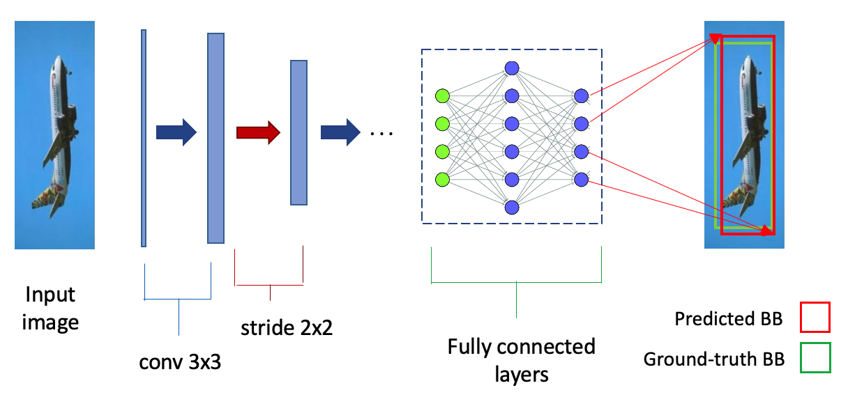
Fig. 1: An illustration of the network structure of LocNet. BB stands for bounding box. Refer to text for details.

Segmentation network We use a convolutional autoencoder (CAE) as the baseline segmentation network, which follows an encoding and decoding architecture. Taking 2D images as inputs, the encoding part repeats the conventional convolution + pooling layers to extract high-level latent features. The decoding part reconstructs the segmentation ground truth mask by using transpose / deconvolution layers.

Our CAE model can be regarded as a simplified version of U-Net [18], which is a popular solution for medical image segmentation. Modifications have been made to suit our data and task. First, we reduce the number of convolutional layers to 10 to fit the image size of our data. Second, we replace max pooling layers with average-pooling, as there is no effective implementation of max pooling in SNNs. Moreover, we remove the concatenation operations (skip connections) that connect the encoding and decoding stacks. This modification is aimed to avoid complicated data synchronization between encoder and decoder layers in the converted SNN model.

2.2 Proposed hybrid SNN-ANN co-training

Our proposed ANN and SNN networks are developed under NengoDL [19], which provides a number of spiking and non-spiking neurons. NengoDL also provides a variety of controls for SNNs, including neuron activations, synaptic smoothing applied to each connection, firing rate of each layer, and time steps that images are presented in the model.

Our hybrid ANN-SNN co-training approach is illustrated in Fig. 2. An ANN of the task of interest will be trained first, before being converted to an SNN. Then, the weights of the converted SNNs are updated through an alternating forward-backward fine-tuning procedure. The forward pass is essentially an SNN inference procedure, which uses quantized activation functions (green-color neurons in Fig. 2) to generate spike trains, flowing through the network. The backward pass computes the error between SNN output and the ground-truth, and uses the gradient of the loss w.r.t. the weights to update the network parameters. Spike activation functions are switched to corresponding non-spike functions along the backward pass.

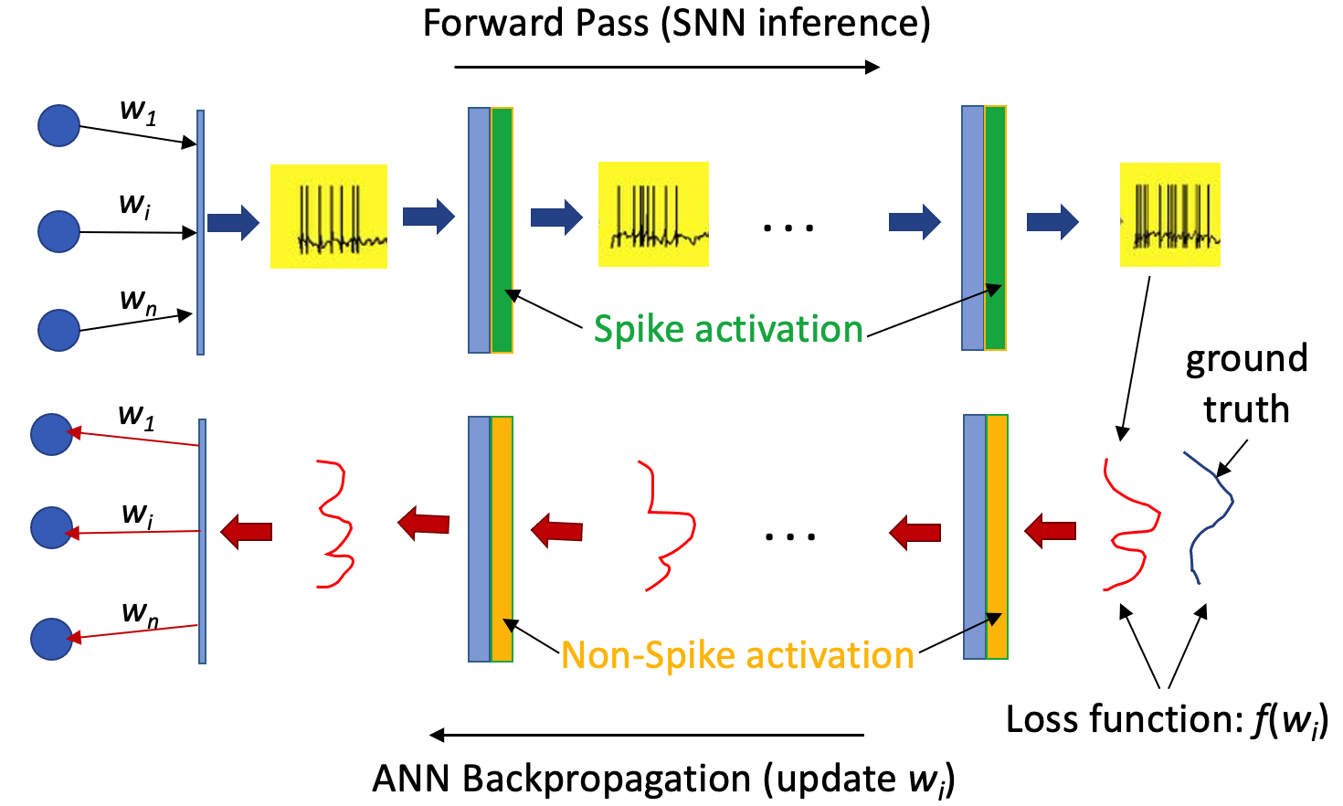
Fig. 2: An illustration of the proposed hybrid ANN-SNN co-training solution. Refer to text for details.

In our LocNet model, we use soft leaky integrate-and-fire (LIF) neurons proposed by Hunsberger and Eliasmith [20, 19]. Extended from LIF, soft LIF neurons have smoothing operations applied around the firing threshold. As explained in [20], the LIF neuron dynamics are defined by the following equation:

$$\tau_{RC}\frac{dv(t)}{dt}=-v(t)+J(t)$$ (1)

where the membrane voltage is $v(t)$, the input current is $J(t)$, and $\tau_{RC}$ represents the membrane time constant. The neuron fires a spike when the voltage $V_{th}=1$. The voltage is then set and remains at zero until a refractory period of $\tau_{ref}$ has passed. To solve for the steady-state firing rate the authors set a constant input current given by $J(t)=j$ which produces this equation:

$$r(j)=\begin{bmatrix}\tau_{ref}-\tau_{RC}\log(1+\frac{V_{th}}{\rho(j-V_{th})})\end{bmatrix}^{-1}$$ (2)

where $\rho(x)=\max(x,0)$. However, as $j\rightarrow 0_{+}$, the steady-state equation’s derivative approaches infinity. To counteract this, the authors set $\rho(x)=\gamma\log(\begin{bmatrix}1+e^{x/\gamma}\end{bmatrix})$. This allows for control over the smoothing that is applied where $\rho(x)\rightarrow\max(x,0)$ as $\gamma\rightarrow 0$. As a result from the smoothing, gradient-based backpropagation can now be carried out to train the network. This design makes the conversion from ANN to SNN rather straightforward, removing the need of complicated thresholding or weight normalization steps in many conversion algorithms. In this work, we take advantage of the convenience brought by this soft LIF model to switch between ANN and SNN to fine-tune both. For our LocNet, we use the mean squared error (MSE) function as the network loss.

In our CAE model, we use the rectified linear neurons in NengoDL, whose activity scales linearly with the current, unless it passes below zero, at which point the neural activity will stay at zero. It should be noted SNNs’ currents are either positive or zero. The gradient of rectified linear neurons is 1 for positive currents and 0 for when the current equals zero. The loss function for our CAE model is set to a weighted combination of binary cross entropy (BCE) and the Dice loss. The contribution is set to 0.5 for each loss component.

NengoDL’s SNN simulator was used to run models as SNNs and collect execution results. When using the simulator, we switch the non-spiking neurons to their spiking counterparts. In LocNet, the soft LIF neurons are switched to spiking LIF neurons while in the CAE model the Rectified Linear neurons are replaced by the Spiking Rectified Linear version. In order to make fair and consistent comparisons, the hyperparameters were maintained the same for the ANN, SNN and hybrid ANN-SNN of the same network.

3 Implementation details

The data for object localization is the airplane subset of Caltech-101 [21]. There are in total 800 images of airplanes with the size of 300$\times$200 pixels. Each image is accompanied with four real-valued numbers that make up the bounding box of the airplane.

The image segmentation task in this work is to extract human brain Hippocampi from magnetic resonance images (MRIs). The data used were obtained from the ADNI database (http://adni.loni.usc.edu), and extracted in our previous work [22, 23]. In total, 110 base-line T1-weighted whole brain MRI images from different subjects along with their hippocampus masks were downloaded. Due to the fact that the hippocampus only occupies a very small part of the whole brain and its position in the whole brain is relatively fixed, we roughly cropped the right face of the hippocampus of each subject and use them as the input for segmentation. The size of the cropping box is $24\times 56\times 48$.

3.1 Training and testing

In SNNs, firing rates play an important role in determining the total energy consumption in the model as well as how information is passed down throughout the network. NengoDL provides two different ways to set the firing rates at network layers: post-training scaling and regularizing during training. The former allows us to apply a linear scale to the inputs of all the neurons and then scale down the outputs with the same rate. The latter is used to directly optimize the firing rates towards certain target values we specify.

LocNet training In the experiments of LocNet, we randomly chose 90% of the data for training while the other 10% were used for testing. Our ANN model was trained with NengoDL’s soft LIF neurons with a smoothing factor of 0.005. The firing rates were regularized during training with a target rate of 250 Hz. Different weights were assigned to the layers in the regularization. As the output layer is the most important, we set its weight to 1. Other layers are less important so we set each of their loss weights to 0.01. Our ANN model was trained for 50 epochs using the Adam optimizer with a learning rate of 0.01.

For hybrid training, the same firing rate regularization technique was used to keep the neurons firing at around 250 Hz. The soft LIF neurons in ANN were replaced with our hybrid soft LIF neurons. In addition to this change, a synapse of 0.005 seconds was added to all connections in the network. The hybrid model was trained for 7 epochs which was determined by an early stopping process. The learning rate was also decreased to 0.001.

CAE training Our dataset to train our CAE network consists of 5280 2D images and masks of the right face of the hippocampus. 4780 of these were used for training while 500 were used for testing. The ReLU activations were swapped out for NengoDL’s Rectified Linear neurons during training. Firing rate scaling was used on these neurons with a scaling factor of 1000. The ANN was trained for 100 epochs using the Adam optimizer and the learning rate was set to 0.00001.

In the hybrid training step, the Rectified Linear neurons were replaced with our hybrid Rectified Linear neurons. A post-training scaling factor of 1000 was also used on both neuron types during training to keep results consistent. A synaptic filter of 0.005 seconds was added to the output of all spiking neurons. Finally, an early stopping technique was used and trained the model for an additional 13 epochs.

4 Experiments and Results

In this section, we present and evaluate the experimental results for the proposed models.

4.1 Object localization

Intersection over Union (IoU) is used to evaluate the object localization networks. IoU measures how closely two sets of elements overlap, and it is defined as the ratio of the overlap area to the combined area of prediction and ground-truth.

Three network models are compared in this experiment. The first is the pure ANN (LocNet) model, which is built and trained with standard CNN components. The second is the SNN directly converted from the ANN (converted SNN). The third one is our hybrid SNN, which is fine-tuned upon the converted SNN with our hybrid training approach. The three models use the same hyperparameters. For SNN models, the soft LIF rate neurons are switched to spiking LIF neurons during testing. Firing rate regularization is used to identify optimal firing rate for the two SNN models.

Model	Mean IoU	Avg. Firing Rate
pure ANN (LocNet)	0.8945	N/A
converted SNN	0.7431	174.5583 Hz
hybrid SNN	0.8253	137.5238 Hz

Table 1: Results from the three localization models.

Table 1 shows the results obtained from the three models. The baseline ANN model achieves a mean IoU of 0.8945. When converted to SNN, the network accuracy drops to 0.7278. Our hybrid fine-tuning procedure is able to improve the performance, measured by IoU, to 0.8253. In addition, our hybrid SNN obtains a slightly smaller average firing rate than the converted version, which poses an advantage from the energy consumption perspective. We believe this is partly due to the weighted regularization terms that are added to the loss function for each layer in the network. The regularization urges the network to implicitly learn the scaling factor to the weights instead of applying a post-scaling in the inference stage for the SNN. Learning an optimized scaling factor for each layer results in optimizing the firing rates.

4.2 Hippocampus segmentation

Dice ratio is used as the performance metric to measure the overlap between the automatic segmentation and the ground truth mask. The results of the competing models are shown in Table 2. Similar to the previous experiment, we have pure ANN, converted SNN, and hybrid SNN as the competing models. All networks use the same set of hyper-parameters. For the firing rates, we use the post-training scaling approach and empirically set the same scaling factor of 1000 for all neurons. We chose not to use firing rate regularization due to the difficulty of setting up appropriate contribution weights.

The baseline pure ANN model was able to achieve a Dice coefficient of 0.8221. The converted model, however, suffers from a large performance loss, only achieving a Dice score of 0.4859. After going through the hybrid fine-tuning process, the hybrid SNN model was able to bring the Dice score back to 0.7648. This clearly demonstrates the effectiveness of the proposed hybrid fine-tuning strategy.

Model	Dice	Avg. Firing Rate
pure ANN (CAE)	0.8221	N/A
converted SNN	0.4859	708.2347 Hz
hybrid SNN	0.7648	731.3800 Hz

Table 2: Results from the three segmentation models.

To visualize the effects of hybrid fine-tuning, we look into a number of slices and compare the masks generated from the three models. Fig. 3 shows a typical example, where (a) and (b) are the input slice and the ground-truth mask. Fig 3.(c), (d) and (e) show the network outputs (probabilistic masks) for ANN, converted SNN and hybrid SNN, respectively. The mask from the ANN matches the ground-truth rather well. The mask from converted SNN, however, contains many artifacts, leading to a poor Dice score after thresholding. The hybrid fine-tuning is able to correct the artifacts and significantly improve the segmentation performance for the SNN model.

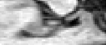
(a) Input slice

(b) Ground-truth

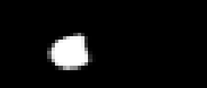
(c) ANN

(d) Converted SNN

(e) Hybrid SNN

Fig. 3: An example of input slice and segmentation results.

5 Conclusions

In this work, we present a hybrid ANN-SNN fine-tuning scheme. Our approach is fairly general and can potentially be applied to many convolutional networks implemented using the soft LIF neurons or the rectified linear neurons. We take object localization and image segmentation as testbed applications, and the effectiveness of our approach is well demonstrated. Exploring more network applications, as well as developing new co-training solutions are our next steps.

References

- [1] Kaushik Roy, Akhilesh Jaiswal, and Priyadarshini Panda, “Towards spike-based machine intelligence with neuromorphic computing,” Nature, vol. 575, no. 7784, pp. 607–617, 2019.
- [2] Mike Davies, Andreas Wild, Garrick Orchard, Yulia Sandamirskaya, Gabriel A Fonseca Guerra, Prasad Joshi, Philipp Plank, and Sumedh R Risbud, “Advancing neuromorphic computing with loihi: A survey of results and outlook,” Proceedings of the IEEE, vol. 109, no. 5, pp. 911–934, 2021.
- [3] Jun Haeng Lee, Tobi Delbruck, and Michael Pfeiffer, “Training deep spiking neural networks using backpropagation,” Frontiers in neuroscience, vol. 10, pp. 508, 2016.
- [4] Colton C Smith, “The evaluation of current spiking neural network conversion methods in radar data,” M.S. thesis, Ohio University, 2021.
- [5] Peter U. Diehl, Daniel Neil, Jonathan Binas, Matthew Cook, Shih-Chii Liu, and Michael Pfeiffer, “Fast-classifying, high-accuracy spiking deep networks through weight and threshold balancing,” pp. 1–8, 2015.
- [6] Bodo Rueckauer, Iulia-Alexandra Lungu, Yuhuang Hu, and Michael Pfeiffer, “Theory and tools for the conversion of analog to spiking convolutional neural networks,” arXiv preprint arXiv:1612.04052, 2016.
- [7] Abhronil Sengupta, Yuting Ye, Robert Wang, Chiao Liu, and Kaushik Roy, “Going deeper in spiking neural networks: Vgg and residual architectures,” Frontiers in Neuroscience, vol. 13, 2019.
- [8] Ye Yue, Marc Baltes, Nidal Abujahar, Tao Sun, Charles D Smith, Trevor Bihl, and Jundong Liu, “Hybrid spiking neural network fine-tuning for hippocampus segmentation,” in ISBI. IEEE, 2023.
- [9] Sumit B Shrestha and Garrick Orchard, “Slayer: Spike layer error reassignment in time,” Advances in neural information processing systems, vol. 31, 2018.
- [10] Yujie Wu, Lei Deng, Guoqi Li, Jun Zhu, and Luping Shi, “Spatio-temporal backpropagation for training high-performance spiking neural networks,” Frontiers in neuroscience, vol. 12, pp. 331, 2018.
- [11] Nitin Rathi, Gopalakrishnan Srinivasan, Priyadarshini Panda, and Kaushik Roy, “Enabling deep spiking neural networks with hybrid conversion and spike timing dependent backpropagation,” 2020.
- [12] Yuhang Li, Yufei Guo, Shanghang Zhang, Shikuang Deng, Yongqing Hai, and Shi Gu, “Differentiable spike: Rethinking gradient-descent for training spiking neural networks,” Advances in Neural Information Processing Systems, vol. 34, pp. 23426–23439, 2021.
- [13] Jibin Wu, Yansong Chua, Malu Zhang, Guoqi Li, Haizhou Li, and Kay Chen Tan, “A tandem learning rule for effective training and rapid inference of deep spiking neural networks,” IEEE Transactions on Neural Networks and Learning Systems, pp. 1–15, 2021.
- [14] Seijoon Kim, Seongsik Park, Byunggook Na, and Sungroh Yoon, “Spiking-yolo: Spiking neural network for energy-efficient object detection,” Proceedings of the AAAI Conference on Artificial Intelligence, vol. 34, no. 07, pp. 11270–11277, Apr. 2020.
- [15] Youngeun Kim, Joshua Chough, and Priyadarshini Panda, “Beyond classification: directly training spiking neural networks for semantic segmentation,” arXiv preprint arXiv:2110.07742, 2021.
- [16] Kinjal Patel, Eric Hunsberger, Sean Batir, and Chris Eliasmith, “A spiking neural network for image segmentation,” arXiv preprint arXiv:2106.08921, 2021.
- [17] Ross Girshick, Jeff Donahue, Trevor Darrell, and Jitendra Malik, “Rich feature hierarchies for accurate object detection and semantic segmentation,” in IEEE CVPR, 2014, pp. 580–587.
- [18] Olaf Ronneberger, Philipp Fischer, and Thomas Brox, “U-net: Convolutional networks for biomedical image segmentation,” in International Conference on Medical image computing and computer-assisted intervention. Springer, 2015, pp. 234–241.
- [19] Daniel Rasmussen, “Nengodl: Combining deep learning and neuromorphic modelling methods,” Neuroinformatics, vol. 17, no. 4, pp. 611–628, 2019.
- [20] Eric Hunsberger and Chris Eliasmith, “Spiking deep networks with lif neurons,” 2015.
- [21] Li, Andreeto, Ranzato, and Perona, “Caltech 101,” Apr 2022.
- [22] Yani Chen, Bibo Shi, Zhewei Wang, Pin Zhang, Charles D Smith, and Jundong Liu, “Hippocampus segmentation through multi-view ensemble convnets,” in ISBI. IEEE, 2017, pp. 192–196.
- [23] Yani Chen, Bibo Shi, Zhewei Wang, Tao Sun, Charles D Smith, and Jundong Liu, “Accurate and consistent hippocampus segmentation through convolutional lstm and view ensemble,” in Machine Learning in Medical Imaging (MLMI). Springer, 2017, pp. 88–96.