Learning Fractals by Gradient Descent

Abstract

Fractals are geometric shapes that can display complex and self-similar patterns found in nature (e.g., clouds and plants). Recent works in visual recognition have leveraged this property to create random fractal images for model pre-training. In this paper, we study the inverse problem — given a target image (not necessarily a fractal), we aim to generate a fractal image that looks like it. We propose a novel approach that learns the parameters underlying a fractal image via gradient descent. We show that our approach can find fractal parameters of high visual quality and be compatible with different loss functions, opening up several potentials, e.g., learning fractals for downstream tasks, scientific understanding, etc.

1 Introduction

A fractal is an infinitely complex shape that is self-similar across different scales. It displays a pattern that repeats forever, and every part of a fractal looks very similar to the whole fractal. Fractals have been shown to capture geometric properties of elements found in nature (Mandelbrot and Mandelbrot 1982). In essence, our nature is full of fractals, e.g., trees, rivers, coastlines, mountains, clouds, seashells, hurricanes, etc.

Despite its complex shape, a fractal can be generated via well-defined mathematical systems like iterated function systems (IFS) (Barnsley 2014). An IFS generates a fractal image by “drawing” points iteratively on a canvas, in which the point transition is governed by a small set of $2\times 2$ affine transformations (each with a probability). Concretely, given the current point $\bm{v}^{(t)}\in\mathbb{R}^{2}$, the IFS randomly samples one affine transformation with replacement from the set, and uses it to transform $\bm{v}^{(t)}$ into the next point $\bm{v}^{(t+1)}$. This stochastic step is repeated until a pre-defined number of iterations $T$ is reached. The collection of $\{\bm{v}^{(0)},\cdots,\bm{v}^{(T)}\}$ can then be used to draw the fractal image (see Figure 1 for an illustration). The set of affine transformations thus can be seen as the parameters (or ID) of a fractal.

Motivated by these nice properties, several recent works in visual recognition have investigated generating a large number of fractal images to facilitate model (pre-)training, in which the parameters of each fractal are randomly sampled (Kataoka et al. 2020; Anderson and Farrell 2022). For instance, Kataoka et al. (2020) sampled multiple sets of parameters and treated each set as a fractal class. Within each class, they leveraged the stochastic nature of the IFS to generate fractal images with intra-class variations. They then used these images to pre-train a neural network in a supervised way without natural images and achieved promising results.

In this paper, we study a complementary and inverse problem — given a target image that is not necessarily a fractal, can we find the parameters such that the generated IFS fractal image looks like it? We consider this problem important from at least two aspects. First, it has the potential to find fractal parameters suitable for downstream visual tasks, e.g., for different kinds of image domains. Second, it can help us understand the limitations of IFS fractals, e.g., what kinds of image patterns the IFS cannot generate.

Figure 1: Overview of our approach, which aims to learn the fractal parameters $\mathcal{S}$ so that the generated point sequence by IFS (i.e., $\{\bm{v}^{(0)},\cdots,\bm{v}^{(300)}\}$), after being rendered onto an image, is close to the target image. We learn $\mathcal{S}$ by gradient descent (GD). As shown, after $1000$ GD steps, we can learn high-quality $\mathcal{S}$ to generate images that are visually close to the target one.

We propose a novel gradient-descent-based approach for this problem (see section 4). Given a target image and the (initial) fractal parameters, our approach compares the image generated by the IFS to the target image, back-propagates the gradients w.r.t. the generated image through the IFS, and uses the resulting gradients w.r.t. the parameters to update the fractal parameters. The key insights are three-folded. First, we view an IFS as a special recurrent neural network (RNN) with identity activation functions and stochastic weights. The weights in each recurrent step (i.e., one affine transformation) are not the same, but are sampled with replacement from shared parameters. This analogy allows us to implement the forward (i.e., image generation) and backward (i.e., back-propagation) passes of IFS using deep learning frameworks like PyTorch (Paszke et al. 2019) and TensorFlow (Abadi et al. 2016). Second, the IFS generates a sequence of points, not an image directly. To compare this sequence to the target image and, in turn, calculate the gradients w.r.t. the generated points, we introduce a differentiable rendering module inspired by (Qian et al. 2020). Third, we identify several challenges in optimization and propose corresponding solutions to make the overall learning process stable, effective, and efficient. The learned parameters can thus lead to high-quality fractal images that are visually similar to the target image. We note that besides reconstructing a target image, our approach can easily be repurposed by plugging in other loss functions that return gradients w.r.t. the generated image.

We conduct two experiments to validate our approach. First, given a target image (that is not necessarily a fractal), we find the fractal parameters to reconstruct it and evaluate our approach using the pixel-wise mean square error (MSE). Our approach notably outperforms the baselines. Second, we extend our approach to finding a set of parameters to approximate a set of target images. This can be achieved by replacing the image-to-image MSE loss with set-to-set losses like the GAN loss (Goodfellow et al. 2014). In this experiment, we demonstrate the potential of finding more suitable fractal images for the downstream tasks than the randomly sampled ones (Kataoka et al. 2020; Anderson and Farrell 2022).

Contributions.

We propose a gradient-descent-based approach to find the fractal parameters for a given image. Our approach is stable, effective, and efficient. It can be easily implemented using popular deep learning frameworks. Moreover, it can be easily extended from finding fractal parameters for image reconstruction to other purposes, by plugging the corresponding loss functions. While we mainly demonstrate the effectiveness of our approach using image reconstruction, we respect think it is a critical and meaningful step towards unlocking other potential usages and applicability of fractal images in visual recognition and deep learning. The codes are provided at https://github.com/andytu28/LearningFractals.

2 Related Work

Fractal inversion.

Finding the parameters of a given fractal image is a long-standing open problem (Vrscay 1991; Iacus and La Torre 2005; Kya and Yang 2001; Guérin and Tosan 2005; Graham and Demers 2019). Many approaches are based on genetic algorithms (Lankhorst 1995; Gutiérrez, Cofiño, and Ivanissevich 2000; Nettleton and Garigliano 1994) or moment matching (Vrscay and Roehrig 1989; Forte and Vrscay 1995). Our approach is novel by tackling the problem via gradient descent and can be easily implemented using deep learning frameworks. We mainly focus on image reconstruction in the image/pixel space, while other ways of evaluation might be considered in the literature.

Fractal applications.

Several recent works leveraged fractals to generate geometrically-meaningful synthetic data to facilitate neural network training (Hendrycks et al. 2021; Baradad Jurjo et al. 2021; Ma et al. 2021; Anderson and Farrell 2022; Kataoka et al. 2020; Gupta, O’Connell, and Egger 2021; Nakashima et al. 2021). Some other works leveraged the self-similar property for image compression, for example, by partitioned IFS (Fisher 1994), which resembles the whole image with other parts of the same image (Pandey and Singh 2015; AL-Bundi and Abd 2020; Jacquin et al. 1992; Al-Bundi, Al-Saidi, and Al-Jawari 2016; Venkatasekhar, Aruna, and Parthiban 2013; Menassel, Nini, and Mekhaznia 2018; Poli et al. 2022). Fractals have also been used in other scientific fields such as diagnostic imaging (Karperien et al. 2008), 3D modeling (Ullah et al. 2021), optical systems (Sweet, Ott, and Yorke 1999), biology (Otaki 2021; Enright and Leitner 2005), etc. In this paper, we study the inverse problem, which has the potential to benefit these applications.

Fractals and neural networks.

Fractals also inspire neural network (NN) architecture designs (Larsson, Maire, and Shakhnarovich 2016; Deng, Yu, and Long 2021) and help the understanding of underlying mechanisms of NNs (Camuto et al. 2021; Dym, Sober, and Daubechies 2020). Specifically, some earlier works (Kolen 1994; Tino and Dorffner 1998; Tino, Cernansky, and Benuskova 2004) used the IFS formulation to understand the properties of recurrent neural networks (RNNs). These works are starkly different from ours in two aspects. First, we focus on the inverse problem of fractals. Second, we formulate an IFS as a special RNN to facilitate solving the inverse problem via gradient descent. We note that Stark (1991) formulated an IFS as sparse feed-forward networks but not for solving the inverse problem.

Inversion of generative models.

The problem we studied is related to the inversion of generative models such as GANs (Zhu et al. 2016; Xia et al. 2021). The goal is to find the latent representation of GANs for a given image that is not necessarily generated by GANs. Our problem has some unique challenges since the fractal generation process is stochastic and not directly end-to-end differentiable.

3 Background

Input : Fractal parameter $\mathcal{S}$, # of iterations $T$, an initial point $\bm{v}^{(0)}\in\mathbb{R}^{2}$

3 for $t\leftarrow 1$ to $T$ do

4       Sample $(\bm{A}^{(t)},\bm{b}^{(t)})$ from $\mathcal{S}$

5       $\bm{v}^{(t)}=\bm{A}^{(t)}\bm{v}^{(t-1)}+\bm{b}^{(t)}$

6 end for

Output : $\{\bm{v}^{(0)},\cdots,\bm{v}^{(T)}\}$

See section 3 for details.

Algorithm 1 IFS generation process.

See section 3 for details.

Input : Fractal embedding $\{\bm{S}_{\text{A}},\bm{S}_{\text{b}}\}$, # of iterations $T$, an initial point $\bm{v}^{(0)}\in\mathbb{R}^{2}$

3 Sample index sequence ${\bm{z}}=[z^{(1)},\cdots,z^{(t)}]$;

4 for $t\leftarrow 1$ to $T$ do

5       $\bm{v}^{(t)}=\texttt{mat}(\bm{S}_{\text{A}}[:,z^{(t)}])\bm{v}^{(t-1)}+\bm{S}_{\text{b}}[:,z^{(t)}]$;

6 end for

Output : $\{\bm{v}^{(0)},\cdots,\bm{v}^{(T)}\}$

See subsection 4.2 for details.

Algorithm 2 IFS generation process via the FE layer.

See subsection 4.2 for details.

We first provide the background about fractal generation via Iterated Function Systems (IFS) (Barnsley 2014). As briefly mentioned in section 1, an IFS can be thought of as “drawing” points iteratively on a canvas. The point transition is governed by a small set of $2\times 2$ affine transformations $\mathcal{S}$:

$$\mathcal{S}=\left\{\left(\bm{A}_{n}\in\mathbb{R}^{2\times 2},\bm{b}_{n}\in\mathbb{R}^{2},p_{n}\in\mathbb{R}\right)\right\}_{n=1}^{N}.$$ (1)

Here, an $(\bm{A}_{n},\bm{b}_{n})$ pair specifies an affine transformation:

$$\bm{A}_{n}{\bm{v}}+\bm{b}_{n},$$ (2)

which transforms a 2D position $\bm{v}\in\mathbb{R}^{2}$ to a new position. The $p_{n}$ in Equation 1 is the corresponding probability of each transformation, i.e., $\sum_{n}p_{n}=1$ and $p_{n}\geq 0,\forall n\in[N]$. $N$ is typically $2\sim 10$.

Given $\mathcal{S}$, an IFS generates an image as follows. Starting from an initial point ${\color[rgb]{1,0,0}\bm{v}^{(0)}}\in\mathbb{R}^{2}$, an IFS repeatedly samples a transformation $(\bm{A}^{(t)},\bm{b}^{(t)})$ from $\{(\bm{A}_{n},\bm{b}_{n})\}_{n=1}^{N}$ with replacement following the probability $\{p_{n}\}_{n=1}^{N}$, and applies

$${\color[rgb]{1,0,0}\bm{v}^{(t)}}=\bm{A}^{(t)}{\color[rgb]{1,0,0}\bm{v}^{(t-1)}}+\bm{b}^{(t)}$$ (3)

to arrive at the next 2D point. This stochastic process can continue forever, but in practice we set a pre-defined number of iterations $T$. The traveled points $\{\bm{v}^{(0)},\cdots,\bm{v}^{(T)}\}$ are then used to synthesize a fractal image. For example, one can quantize them into integer pixel coordinates and render each pixel as a binary (i.e., $1$) value on a black (i.e., $0$) canvas. We summarize the IFS fractal generation process in algorithm 1. Due to the randomness in sampling $(\bm{A}^{(t)},\bm{b}^{(t)})$, one $\mathcal{S}$ can create different but geometrically-similar fractal images. We call $\mathcal{S}$ the fractal parameters.

Simplified parameters.

We follow (Kataoka et al. 2020; Anderson and Farrell 2022) to set $p_{n}$ by the determinant of the corresponding $\bm{A}_{n}$. That is, $p_{n}\propto|\texttt{det}(\bm{A}_{n})|$. In the following, we will ignore $p_{n}$ when defining $\mathcal{S}$:

$$\mathcal{S}=\left\{\left(\bm{A}_{n},\bm{b}_{n}\right)\right\}_{n=1}^{N}.$$ (4)

4 End-to-End Learnable Fractals by Gradient Descent

In this paper, we study the problem: given a target image, can we find the parameters $\mathcal{S}$ such that the generated IFS fractal image looks like it? Let us first provide the problem definition and list the challenges, followed by our algorithm and implementation.

4.1 Problem and challenges

Problem.

Given a gray-scaled image $\bm{I}\in[0,1]^{H\times W}$, where $H$ is the height and $W$ is the width, we want to find the fractal parameters $\mathcal{S}$ (cf. Equation 4) such that the generated IFS fractal image $\bm{I}^{\prime}\in[0,1]^{H\times W}$ is close to $\bm{I}$. We note that $\bm{I}$ may not be a fractal image generated by an IFS.

Let us denote the IFS generation process by $\bm{I}^{\prime}=G(\mathcal{S})$, and the image-to-image loss function by $\mathcal{L}$. This problem can be formulated as an optimization problem:

$$\min_{\mathcal{S}}\mathcal{L}(G(\mathcal{S}),\bm{I}).$$ (5)

We mainly consider the pixel-wise square loss $\mathcal{L}(\bm{I}^{\prime},\bm{I})=\|\bm{I}^{\prime}-\bm{I}\|_{2}^{2}$, but other loss functions can be easily applied. We note that $G$ is stochastic, and we will discuss how to deal with it in subsection 4.4.

Goal.

We aim to solve Equation 5 via gradient descent (GD) — as shown in Equation 3, each iteration in IFS is differentiable. Specifically, we aim to develop our algorithm as a module such that it can be easily implemented by modern deep learning frameworks like PyTorch and TensorFlow. This can largely promote our algorithm’s usage, e.g., to combine with other modules for end-to-end training.

It is worth mentioning that while $\bm{I}^{\prime}$ depends on $\{p_{n}\}_{n=1}^{N}$ and $\{p_{n}\}_{n=1}^{N}$ depends on $\{\bm{A}_{n}\}_{n=1}^{N}$ (cf. Equation 4), we do not include this path in deriving the gradients w.r.t. $\{\bm{A}_{n}\}_{n=1}^{N}$ for simplicity.

Challenges.

We identify several challenges in achieving our goal.

• First, it is nontrivial to implement and parallelize the IFS generation process (for multiple fractals) using modern deep learning frameworks.

• Second, the whole IFS generation process is not immediately differentiable. Specifically, an IFS generates a sequence of points, not directly an image. We need to back-propagate the gradients from an image to the points.

• Third, there are several technical details to make the optimization effective and stable. For example, an IFS is stochastic. The IFS generation involves hundreds or thousands of iterations (i.e., $T$); the back-propagation would likely suffer from exploding gradients.

In the rest of this section, we describe our solution to each of these challenges. We provide a summarized pipeline of our approach in Figure 1.

(a)

(b)

Figure 2: (a) Fractal embedding layer in subsection 4.2. We show a case of $T=3$ and batch size $=2$. The purple dashed lines indicate the point transition (like the hidden vector in RNNs). (b) Differentiable rendering in subsection 4.3. We show that the gradients w.r.t. the rendered image can be translated into 2D gradient vectors w.r.t. the IFS points, i.e., $\nabla_{\bm{v}^{(t)}}\mathcal{L}\in\mathbb{R}^{2},\forall t\in\{1,\cdots,T\}$ (zoom-in for better resolutions).

4.2 Fractal generation as a deep learning model

IFS as an RNN.

We start with how to implement the IFS fractal generation process as a deep learning model. We note that an IFS performs Equation 3 for $T$ iterations. Every iteration involves an affine transformation, which is sampled with replacement from the fractal parameters $\mathcal{S}$. Let us assume that $\mathcal{S}$ contains only one pair $(\bm{A},\bm{b})$, then an IFS can essentially be seen as a special recurrent neural network (RNN), which has an identity activation function but no input vector:

$$\bm{v}^{(t)}=\bm{A}\bm{v}^{(t-1)}+\bm{b}.$$ (6)

Here, $\bm{v}^{(t)}$ is the RNN’s hidden vector. That is, an IFS can be implemented like an RNN if it contains only one transformation. In the following, we extend this notion to IFS with multiple transformations.

IFS rearrangement.

To begin with, let us rearrange the IFS generation process. Instead of sampling an affine transformation from $\mathcal{S}$ at each of the $T$ IFS iterations, we choose to sample all $T$ of them before an IFS starts. We can do so because the sampling is independent of the intermediate results of an IFS. Concretely, according to $\{p_{n}\}_{n=1}^{N}$, we first sample an index sequence ${\bm{z}}=[z^{(1)},\cdots,z^{(t)}]$, in which $z^{(t)}\in\{1,\cdots,N\}$ denotes the index of the sampled affine transformation from $\mathcal{S}$ at iteration $t$. With the pre-sampled ${\bm{z}}$, we can perform an IFS in a seemingly deterministic way. This is reminiscent of the re-parameterization trick commonly used in generative models (Kingma and Welling 2013).

Fractal embedding layer.

We now introduce a fractal embedding (FE) layer, which leverages the rearrangement to implement an IFS like an RNN. The FE layer has two sets of parameters, $\bm{S}_{\text{A}}\in\mathbb{R}^{4\times N}$ and $\bm{S}_{\text{b}}\in\mathbb{R}^{2\times N}$, which record all the parameters in $\mathcal{S}$ (cf., Equation 4). Specifically, the $n$^th column of $\bm{S}_{\text{A}}$ (denoted as $\bm{S}_{\text{A}}[:,n]$) records the $2\times 2$ parameters of $\bm{A}_{n}$; i.e., $\bm{A}_{n}=\texttt{mat}(\bm{S}_{\text{A}}[:,n])$, where mat is a reshaping operation from a column vector into a matrix. The $n$^th column of $\bm{S}_{\text{b}}$ (denoted as $\bm{S}_{\text{b}}[:,n]$) records $\bm{b}_{n}$, i.e., $\bm{b}_{n}=(\bm{S}_{\text{b}}[:,n])$. Let us define one more notation $\textbf{1}_{z^{(t)}}\in\mathbb{R}^{N}$, which is an $N$-dimensional one-hot vector whose $z^{(t)}$^th element is $1$. With these parameters and notation, the FE layer carries out the IFS computation at iteration $t$ (cf. Equation 3) as follows

$$\textsc{FE}(z^{(t)},\bm{v}^{(t-1)};\{\bm{S}_{\text{A}},\bm{S}_{\text{b}}\})$$

$$=\texttt{mat}(\bm{S}_{\text{A}}\textbf{1}_{z^{(t)}})\bm{v}^{(t-1)}+\bm{S}_{\text{b}}\textbf{1}_{z^{(t)}}$$

$$=\texttt{mat}(\bm{S}_{\text{A}}[:,z^{(t)}])\bm{v}^{(t-1)}+\bm{S}_{\text{b}}[:,z^{(t)}]$$ (7)

$$=\bm{A}^{(t)}\bm{v}^{(t-1)}+\bm{b}^{(t)}.$$

That is, the FE layer takes the index of the sampled affine transformation of iteration $t$ (i.e., $z^{(t)}$) and the previous point $\bm{v}^{(t-1)}$ as input, and outputs the next point $\bm{v}^{(t)}$. To perform an IFS for $T$ iterations, we only need to call the FE layer recurrently for $T$ times. This analogy between IFS and RNNs makes it fairly easy to implement the IFS generation process in modern deep learning frameworks. Please see algorithm 2 for a summary.

Extension to mini-batch versions.

The FE layer can easily be extended into a mini-batch version to generate multiple fractal images, if they share the same fractal parameters $\mathcal{S}$. See Figure 2 (a) for an illustration. Interestingly, even if the fractal images are based on different fractal parameters, a simple parameter concatenation trick can enable mini-batch computation. Let us consider a mini-batch of size $2$ with fractal parameters $\mathcal{S}_{1}$ and $\mathcal{S}_{2}$. We can combine $\mathcal{S}_{1}$ and $\mathcal{S}_{2}$ into one $\bm{S}_{\text{A}}\in\mathbb{R}^{4\times(2N)}$ and one $\bm{S}_{\text{b}}\in\mathbb{R}^{2\times(2N)}$, where the number of columns in $\bm{S}_{\text{A}}$ and $\bm{S}_{\text{b}}$ are doubled to incorporate the affine transformations in $\mathcal{S}_{1}$ and $\mathcal{S}_{2}$. When sampling the index sequence for each fractal, we just need to make sure that the indices align with the columns of $\bm{S}_{\text{A}}$ and $\bm{S}_{\text{b}}$ to generate the correct fractal images.

4.3 Differentiable rendering

The FE layer enables us to implement an IFS via modern deep learning frameworks, upon which we can enjoy automatic back-propagation to calculate the gradients $\nabla_{\mathcal{S}}\mathcal{L}$ (cf. Equation 5) if we have obtained the gradients $\nabla_{\bm{v}^{(t)}}\mathcal{L},\forall t\in\{1,\cdots,T\}$. However, obtaining the latter is not trivial. An IFS generates a sequence $\{\bm{v}^{(0)},\cdots,\bm{v}^{(T)}\}$ of 2D points, but it is not immediately clear how to render an image $\bm{I}^{\prime}$ such that subsequently we can back-propagate the gradient $\nabla_{\bm{I}^{\prime}}\mathcal{L}(\bm{I}^{\prime},\bm{I})$ to obtain $\nabla_{\bm{v}^{(t)}}\mathcal{L}$.

Concretely, $\nabla_{\bm{I}^{\prime}}\mathcal{L}$ is a 2D tensor of the same size as $\bm{I}^{\prime}$, where $\nabla_{\bm{I}^{\prime}[h,w]}\mathcal{L}\in\mathbb{R}$ indicates if the pixel $[h,w]$ of $\bm{I}^{\prime}$ should get brighter or darker. Let us follow the definition in section 3: IFS draws points on a black canvas. Then if $\nabla_{\bm{I}^{\prime}[h,w]}\mathcal{L}\in\mathbb{R}<0$, ideally we want to have some IFS points closer to or located at $[h,w]$, to make $\bm{I}^{\prime}[h,w]$ brighter. To do so, however, requires a translation of $\nabla_{\bm{I}^{\prime}[h,w]}\mathcal{L}<0$ into a “pulling” force towards $\bm{I}^{\prime}[h,w]$ for some of the points in $\{\bm{v}^{(0)},\cdots,\bm{v}^{(T)}\}$ .

To this end, we propose to draw the IFS points $\{\bm{v}^{(0)},\cdots,\bm{v}^{(T)}\}$ onto $\bm{I}^{\prime}$ using an RBF kernel — every point “diffuses” its mass to nearby pixels. This is inspired by the differentiable soft quantization module (Qian et al. 2020) proposed for 3D object detection. The rendered image $I^{\prime}$ is defined as

$$\bm{I}^{\prime}[h,w]=\sum_{t}\exp(-\left\|[h,w]^{\top}-\bm{v}^{(t)}\right\|_{2}^{2}/\tau),$$

$$h\in[H],w\in[W],$$ (8)

where $\tau>0$ governs the kernel’s bandwidth. This module not only is differentiable w.r.t. $\bm{v}^{(t)}$, but also fulfills our requirement. The closer the IFS points to $[h,w]$ are, the larger the intensity of $\bm{I}^{\prime}[h,w]$ is. Moreover, if $\nabla_{\bm{I}^{\prime}[h,w]}\mathcal{L}<0$, then $\frac{\partial\mathcal{L}}{\partial\bm{I}^{\prime}[h,w]}\times\frac{\partial\bm{I}^{\prime}[h,w]}{\partial\bm{v}^{(t)}}$ will be a 2D vector positively proportional to $(\bm{v}^{(t)}-[h,w]^{\top})$. When GD is applied, this will pull $\bm{v}^{(t)}$ towards $[h,w]^{\top}$. See Figure 2 (b) for an illustration.

Since $\bm{I}^{\prime}[h,w]$ may have a value larger than $1$, we clamp it back to the range $[0,1]$ by $\min(\bm{I}^{\prime}[h,w],1)$.

4.4 Objective and optimization

In subsection 4.2 and subsection 4.3, we present an end-to-end differentiable framework for learning $\mathcal{S}$. In this subsection, we discuss the objective function and present important technical insights to stabilize the optimization.

Objective function.

As pointed out in the subsequent paragraph of Equation 5, since an IFS is stochastic, the objective function in Equation 5 is ill-posed. To tackle this, let us rewrite the stochastic $G(\mathcal{S})$ by $G(\mathcal{S};{\bm{z}})$, in which we explicitly represent the stochasticity in $G(\mathcal{S})$ by ${\bm{z}}$: the sampled index sequence according to $\mathcal{S}$ (see subsection 4.2). We then present two objective functions:

$$\@@unnumbered@section{paragraph}{toc}{Expectation: }\mathbb{E}_{{\bm{z}}\sim\mathcal{S}}\left[\mathcal{L}(G(\mathcal{S},{\bm{z}}),\bm{I})\right],$$

$$\textbf{Fixed: }\mathbb{E}_{{\bm{z}}\in\mathcal{Z}}\left[\mathcal{L}(G(\mathcal{S},{\bm{z}}),\bm{I})\right],$$ (9)

where ${\bm{z}}\sim\mathcal{S}$ indicates that ${\bm{z}}$ is sampled according to $\mathcal{S}$; $\mathcal{Z}$ is a set of pre-sampled fixed sequences. For instance, we can sample $\mathcal{Z}$ according to the initial $\mathcal{S}$ and fix it throughout the optimization process. The Expectation objective encourages every ${\bm{z}}\sim\mathcal{S}$ to generate $\bm{I}$. The learned $\mathcal{S}$ thus would easily generate images $\bm{I}^{\prime}$ close to $\bm{I}$, but the diversity among $\bm{I}^{\prime}$ might be limited. The Fixed objective is designed to alleviate this limitation by only forcing a (small) set of fixed sequences $\mathcal{Z}$ to generate $\bm{I}$. However, since $\mathcal{Z}$ is pre-sampled, their probability of being sampled from the learned $\mathcal{S}$ might be low. Namely, it might be hard for the learned $\mathcal{S}$ to generate images like $\bm{I}$. We evaluate both in section 5.

Optimization.

We apply mini-batch stochastic gradient descent (SGD) to optimize the objectives w.r.t. $\mathcal{S}$ in Equation 9. To avoid confusion, we use “iteration” for the IFS generation process, and “step” for the SGD optimization process. The term “stochastic” refers to sampling a mini-batch of ${\bm{z}}$ at every optimization step from either $\mathcal{S}$ or $\mathcal{Z}$, generating the corresponding fractal images $\bm{I}^{\prime}$ by IFS, and calculating the average gradients w.r.t. $\mathcal{S}$.

Figure 3: The training loss along the steps of SGD w/ and w/o adding random noise to the fractal parameters $\mathcal{S}$. We add a Gaussian noise $\sim\mathcal{N}(0,0.1)$ to each element of the fractal parameters $\mathcal{S}$ every $5$ SGD steps. This makes the final loss lower and the optimization robust. (The “shaded” area is the standard deviation across different random seeds.)

We note that unlike neural networks that are mostly over-parameterized, $\mathcal{S}$ has much fewer, usually tens of parameters. This somehow makes the optimization harder. Specifically, we found that the optimization easily gets stuck at poor local minima. (In contrast, over-parameterized models are more resistant to it (Du et al. 2019; Allen-Zhu, Li, and Liang 2019; Arora et al. 2019).) To resolve this, whenever we calculate the stochastic gradients, we add a small Gaussian noise to help the current parameters escape local minima, inspired by (Welling and Teh 2011). Figure 3 shows that this design stabilizes the optimization process and achieves lower loss. More results are in section 5.

Reparameterized $\mathcal{S}$.

In the extreme case where $\mathcal{S}$ contains only one affine transformation $(\bm{A},\bm{b})$, recurrently applying it multiple times could easily result in exploding gradients when the maximum singular value of $\bm{A}$ is larger than $1$ (Pascanu, Mikolov, and Bengio 2013). This problem happens when $\mathcal{S}$ contains multiple affine transformations as well, if most of the matrices have such a property. To avoid it, we follow (Anderson and Farrell 2022) to decompose “each” $\bm{A}$ in $\mathcal{S}$ into rotation, scaling, and flipping matrices

$${\bm{A}=\underbrace{\begin{bmatrix}\text{cos}(\theta)&-\text{sin}(\theta)\\ \text{sin}(\theta)&\text{cos}(\theta)\end{bmatrix}}_{\text{rotation}}\underbrace{\begin{bmatrix}\sigma_{1}&0\\ 0&\sigma_{2}\end{bmatrix}}_{\text{scaling}}\underbrace{\begin{bmatrix}\text{cos}(\phi)&-\text{sin}(\phi)\\ \text{sin}(\phi)&\text{cos}(\phi)\end{bmatrix}}_{\text{rotation}}\underbrace{\begin{bmatrix}d_{1}&0\\ 0&d_{1}\end{bmatrix}}_{\text{flipping}},}$$ (10)

where $\sigma_{1},\sigma_{2}\geq 0;d_{1},d_{2}\in\{-1,1\}$. That is, $\bm{A}$ is reparameterized by $\{\theta,\phi,\sigma_{1},\sigma_{2},d_{1},d_{2}\}$. We note that Anderson and Farrell (2022) used this decomposition to sample $\bm{A}$. The purpose was to generate diverse fractal images for pre-training. Here, we use this decomposition for a drastically different purpose: to stabilize the optimization of $\bm{A}$. We leverage one important property — $\max(\sigma_{1},\sigma_{2})$ is exactly the maximum singular value of $\bm{A}$ — and clamp both $\sigma_{1}$ and $\sigma_{2}$ into $[0,1]$ to avoid exploding gradients.

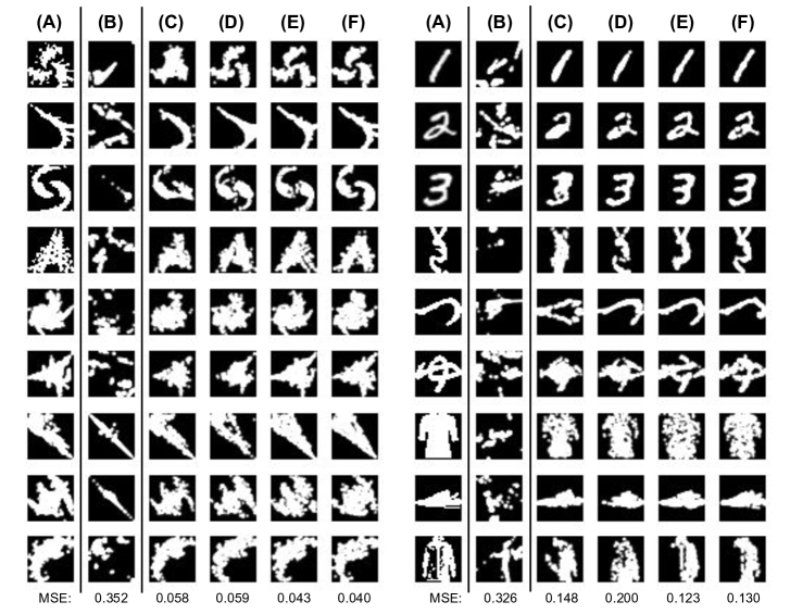
Figure 4: Image reconstruction examples. Left: FractalDB images. Right: MNIST (row 1-3), KMNIST (row 4-6), and FMNIST images (row 7-9). (A): the target images. (B): an inverse encoder baseline. (C-F): variants of our approach (corresponding to the “Index” column in Table 1). The last row shows two examples and the corresponding MSE.

Table 1: Averaged MSE (mean$\pm$std over $3$ runs) of image reconstruction on FractalDB/MNIST/KMNIST/FMNIST dataset.

Index	Method	Objective	Clamp	Noisy	FractalDB	MNIST	KMNIST	FMNIST
(B)	Inverse encoder	-	-	-	$0.3889\pm 0.0000$	$0.1724\pm 0.0000$	$0.3016\pm 0.0000$	$0.3658\pm 0.0000$
(C)	Ours	Fixed	✗	✗	$0.0790\pm 0.0006$	$0.0475\pm 0.0012$	$0.1023\pm 0.0016$	$0.0692\pm 0.0010$
(D)		Fixed	✓	✗	$0.0752\pm 0.0027$	$0.0312\pm 0.0002$	$0.0979\pm 0.0008$	$0.0765\pm 0.0034$
(E)		Expectation	✓	✗	$0.0630\pm 0.0008$	$0.0223\pm 0.0004$	$0.0826\pm 0.0010$	$0.0547\pm 0.0005$
(F)		Expectation	✓	✓	$\mathbf{0.0617\pm 0.0009}$	$\mathbf{0.0202\pm 0.0005}$	$\mathbf{0.0781\pm 0.0015}$	$\mathbf{0.0538\pm 0.0006}$
	Ours (w/o Reparam. $\mathcal{S}$)	Expectation	✓	✓	Exploded	Exploded	Exploded	Exploded

4.5 Extension

Besides the pixel-wise square loss $\mathcal{L}(\bm{I}^{\prime},\bm{I})=\|\bm{I}^{\prime}-\bm{I}\|_{2}^{2}$, our approach can easily be compatible with other loss functions on $\bm{I}^{\prime}$. The loss may even come from a downstream task. In subsection 5.3, we experiment with one such extension. Given a set of images $\{\bm{I}_{m}\}_{m=1}^{M}$, we aim to learn a set of fractal parameters $\{\mathcal{S}_{j}\}_{j=1}^{J}$ such that their generated images are distributionally similar to $\{\bm{I}_{m}\}_{m=1}^{M}$. We apply a GAN loss (Goodfellow et al. 2014). In the optimization process, we train a discriminator to tell real images from generated images, and use it to provide losses to the generated images.

5 Experiments

We conduct two experiments to quantitatively and qualitatively validate our approach and design choices. These include (1) image reconstruction: learning an IFS fractal to reconstruct each given target image by gradient descent, using the mean squared error on pixels; (2) learning fractals with a GAN loss: given a set of target images, extending our approach to learn a set of fractal parameters that generates images with distributions similar to the targets.

We note that we do not intend to compete with other state-of-the-art in these tasks that do not involve fractals. Our experiments are to demonstrate that our learnable fractals can capture meaningful information in the target images. Please see the supplementary material for more details and analyses.

5.1 Setups

Datasets.

We first reconstruct random fractal images generated following FractalDB (Kataoka et al. 2020; Anderson and Farrell 2022). We then consider images that are not generated by fractals, including MNIST (hand-written digits) (LeCun et al. 1998), FMNIST (fashion clothing) (Xiao, Rasul, and Vollgraf 2017), and KMNIST (hand-written characters) (Clanuwat et al. 2018), for both reconstruction and GAN loss experiments. We use $32\times 32$ binarized (black-and-white) images as target images for reconstruction. For the GAN loss experiment, we use the $60K/10K$ training/test images out of $10$ classes in the three non-fractal datasets.

Technical details about fractals.

Throughout the experiments, we sample $\bm{v}^{(0)}$ and initialize $\mathcal{S}$ by the random procedure in (Anderson and Farrell 2022). The number of transformations in $\mathcal{S}$ is fixed to $N=10$, and we set $T=300$ per image. These apply to the FractalDB generation as well.

To learn $\mathcal{S}$ using our proposed method, we set $\tau=1$ (RBF kernel bandwidth) and apply an Adam optimizer (Kingma and Ba 2015). We verify our design choices in the ablation studies of subsection 5.2 and the supplementary material.

5.2 Image reconstruction and ablation study

In the image reconstruction task, our goal is to verify our gradient descent-based method can effectively recover target shapes. Specifically, given a target image, we learn an $\mathcal{S}$ using our proposed approach to reconstruct the target shape by minimizing the mean squared error (MSE) between the generated and the target images. Each $\mathcal{S}$ is learned with a batch size $50$ and a learning rate $0.05$ for $1,000$ SGD steps. As we recover any given target by learning a fractal $\mathcal{S}$, no training and test splits are considered. In this experiment, we generate $2K$ target images using FractalDB, and randomly sample $2K$ target images from each MNIST/FMNIST/KMNIST. For quantitative evaluation, after $\mathcal{S}$ is learned, we generate $100$ images per $\mathcal{S}$ (with different sampled sequences ${\bm{z}}$) and report the minimum MSE to reduce the influence of random sequences. We consider the following variants of our method:

• Using either the Expectation objective or the Fixed objective discussed in subsection 4.4.

• In differentiable rendering (see subsection 4.3), clamping each pixel to be within $[0,1]$ or not.

• Applying the noisy SGD trick or not (see subsection 4.4).

• Learning the reparameterized $\mathcal{S}$ or the original IFS parameters $\mathcal{S}$ (see subsection 4.4).

Besides our variants, we also include an inverse encoder baseline similar to the recent work (Graham and Demers 2019) that learns a ResNet18 (He et al. 2016) to predict the fractal parameters $\mathcal{S}$ given an image (i.e., as a regression problem). We train such a regressor on $20K$ different FractalDB images (using the corresponding $\mathcal{S}$ as labels) and use it on the target images (details are in the supplementary material).

Qualitatively, Figure 4 shows examples of image reconstruction. Our approach works well on fractal shapes. Surprisingly, we can also recover non-fractal datasets to an extent. This reveals that IFS can be more expressive if the parameters are learned in a proper way. By contrast, the inverse encoder cannot recover the target shapes and ends up with poor MSE.

Quantitatively, the reported MSE (averaged over all targets) in Table 1 verifies our design choices of applying the Expectation objective, clamping the rendered images, and applying noisy SGD. Notably, without reparameterization, we can hardly learn $\mathcal{S}$ since the gradients quickly explode.

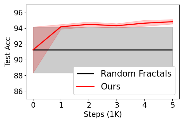
(a) MNIST

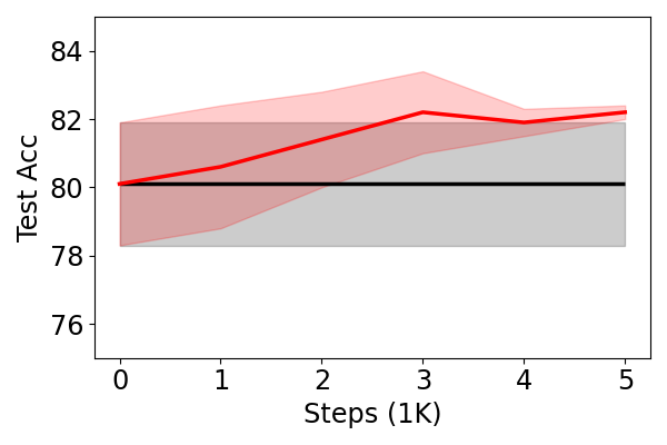
(b) FMNIST

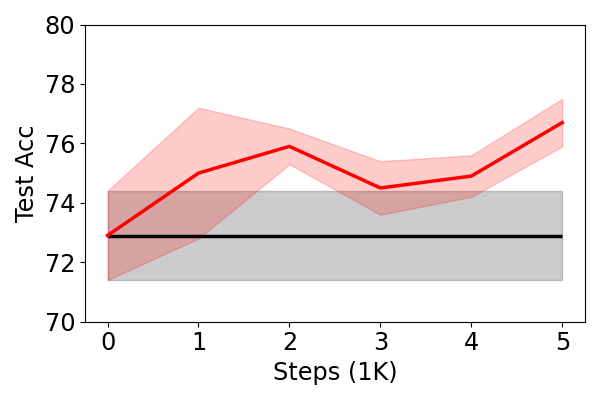
(b) KMNIST

Figure 5: Learning fractals as GANs. We conduct linear evaluations using features pre-trained (for $0\sim 5K$ SGD steps) on the learned/random fractal images. Test accuracy of means (lines) and standard deviations (shades) over $10$ runs are plotted.

5.3 Learning fractals as GAN generators

As discussed in subsection 4.5, our approach is a flexible deep learning module that can be learned with other losses besides MSE. To demonstrate such flexibility, we learn fractals like GANs (Goodfellow et al. 2014) by formulating a set-to-set learning problem — matching the distributions of the images generated from fractals to the distributions of (real) target images. Specifically, we start from $100$ randomly sampled fractals $\mathcal{S}$ and train them on the target training set of MNIST/FMNIST/KMINIST in an unsupervised way using the GAN loss with a discriminator (a binary LeNet (LeCun et al. 1998) classifier). Next, we evaluate the learned fractals by using them for model pre-training (Kataoka et al. 2020).

We argue that if the learned fractals $\mathcal{S}$ can produce image distributions closer to the targets, pre-training on the generated images should provide good features w.r.t. the (real) target images. We expect pre-training on the images generated from the learned $\mathcal{S}$ to yield better features for the target datasets, compared to pre-training on random fractals.

Concretely, we pre-train a $100$-way classifier (using the LeNet architecture again) from scratch. We generate $600$ images from each $\mathcal{S}$ and treat each $\mathcal{S}$ as a pseudo-class following (Kataoka et al. 2020) to form a $100$-class classification problem. Then, we conduct a linear evaluation on the pre-trained features using the real training and test sets.

Figure 5 shows the results, in which we compare pre-training on the random fractals (gray lines) and on the learned fractals (red lines), after every $1K$ SGD steps. As we pre-train $\mathcal{S}$ with more steps, the learned fractals can more accurately capture the target image distribution, evidenced by the better pre-trained features that lead to higher test accuracy. This study shows the helpfulness of our method for pre-training.

6 Conclusion, Limitations, and Future Work

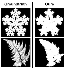
Figure 6: Inversion on complex (fractal) images.

We present a gradient descent-based method to find the fractal parameters for a given image. Our approach is stable, effective, and can be easily implemented using popular deep learning frameworks. It can also be extended to finding fractal parameters for other purposes, e.g., to facilitate downstream vision tasks, by plugging in the corresponding losses.

We see some limitations yet to be resolved. For example, IFS itself cannot handle color images. Our current approach is hard to recover very detailed structures (e.g., Figure 6). We leave them for our future work. We also plan to further investigate our approach on 3D point clouds.

Supplementary Material

We provide details omitted in the main paper.

• Appendix A: additional training details (cf. section 5 of the main paper).

• Appendix B: additional experiments and analyses (cf. section 5 of the main paper).

• Appendix C: additional discussions.

Appendix A Additional Training Details

A.1 Training details for image inversion

We note that for the image inversion experiment, our goal is to learn $\mathcal{S}$ for a given target image. The quantitative error is directly measured between the generated images by the learned $\mathcal{S}$ and the target image.

We provide training details for the inverse encoder baseline (Graham and Demers 2019) we compared to that predicts fractal parameters $\mathcal{S}$ (i.e., as a regression problem) given an input image (cf. subsection 5.2 of the main paper). We first pre-generate $100K$ fractal images from $20K$ different $\mathcal{S}$; each $\mathcal{S}$ has 10 transformations. For each image, its corresponding $\mathcal{S}$ is used as its label (i.e., regression target), and the transformations are ordered by their maximum singular values. Then, we train a ResNet18 to directly output the target $\mathcal{S}$, which has $10\times(4+2)$ dimensions, using the mean squared error (MSE). The ResNet18 is pre-trained on ImageNet, and we train it on fractal inversion for 100 epochs using the SGD optimizer with learning rate $0.05$, momentum $0.9$, weight decay $1\mathrm{e}{-4}$, and batch size $128$. The learning rate is reduced every epoch following the cosine schedule (Loshchilov and Hutter 2017).

The training details of our learnable fractals are as follows. Given a target image, we randomly initialize an $\mathcal{S}$ in its reparameterized form (cf. Equation 10). Then, in all experiments, we use the Adam optimizer with a mini-batch of $50$ sequences (i.e., ${\bm{z}}$) to train $\mathcal{S}$. For the Fixed objective, we randomly sample the $50$ sequences based on the initial $\mathcal{S}$ at the beginning and fix them throughout the training. For the Expectation objective, we sample different $50$ sequences at every training step. Our sequence sampling follows (Anderson and Farrell 2022). We optimize the $\mathcal{S}$ for $1000$ steps, and the learning rate is initialized with $0.05$ and decayed by $0.5$ every $250$ steps.

A.2 Training details for learning fractals as GAN

We note that for this experiment, our goal is to learn a set of $\mathcal{S}$ such that the resulting fractal images can be used to pre-train a LeNet with stronger features. We use supervised pre-training: images generated by each $\mathcal{S}$ are considered as the same class.

We start by randomly sampling 100 different fractals $\mathcal{S}$ (each can be used to generate more fractal images) and gradually adjust them so that the overall distributions of their generated fractal images become closer to the real images in MNIST/FMNIST/KMNIST. To achieve this goal, we plug in the GAN loss to train the 100 fractal $\mathcal{S}$ as a generator. That is, we randomly sample some $\mathcal{S}$ and use them to generate a mini-batch of images. A discriminator network will compare the distribution of the generated images and the real images and compute the GAN loss for updating the generator. In the GAN training, we adopt batch size $16$ and generator learning rate $1\mathrm{e}{-4}$. We use a LeNet as our discriminator and update it once every $10$ training steps of the generator. The discriminator learning rate is $1\mathrm{e}{-5}$.

As we gradually train the $100$ fractals $\mathcal{S}$ to generate images similar to the real data, we expect the generated fractal images to become similar to the real image distributions. We note that this process is unsupervised as GAN training does not require any categorical labels from these datasets.

We adopt a linear probing way to evaluate the quality of the generated images — the generated images should be suitable to pre-train features for MNIST/FMNIST/KMNIST. We evaluate the pre-training performance as we keep updating the $\mathcal{S}$. At every 1K steps of training the 100 fractal $\mathcal{S}$, we use them to generate $60K$ images for pre-training LeNet features. The features are then evaluated by learning a linear classifier (with frozen features) on the real training sets of MNIST/FMNIST/KMNIST. In the linear evaluation, we train the classifier for 100 epochs using SGD with a learning rate $0.001$, momentum $0.9$, and a batch size $128$.

Appendix B Additional Experiments and Analyses

Table 2: Averaged MSE (means$\pm$std over $3$ runs) of our fractal inversion with $N\in{2,6,10}$ transformations.

Dataset	$N=2$	$N=6$	$N=10$
FractalDB	$0.0954\pm 0.0035$	$0.0687\pm 0.0006$	$0.0627\pm 0.0013$
MNIST	$0.0423\pm 0.0013$	$0.0237\pm 0.0015$	$0.0212\pm 0.0009$

B.1 Different numbers of transformations in $\mathcal{S}$

As the number of transformations controls the expressibility of $\mathcal{S}$, we provide an ablation study to investigate its influence on image inversion. We randomly sample $500$ images for FractalDB/MNIST and adopt our best setup (with clamping, the Expectation objective, and noisy SGD) for training with $N=2,6,10$. The averaged MSE is reported in Table 2. The results show that the MSE decreases as $N$ increases, reflecting how $N$ affects the expressive power of $\mathcal{S}$. We conclude that target shapes can be more accurately recovered if more fractal parameters (i.e., $\mathcal{S}$ with more affine transformations) are used.

Table 3: Averaged MSE (means$\pm$std over $3$ runs) of our fractal inversion with Adam or SGD.

Dataset	SGD	Adam
MNIST	$0.0656\pm 0.0014$	$0.0212\pm 0.0009$

B.2 Different optimizers (SGD vs. Adam)

The optimization of fractals is non-trivial and involves several technical details to make it effective and stable. Throughout all our experiments, we adopt the Adam optimizer as we find it particularly effective for learning fractals. We provide the results of our best setup using the SGD optimizer with a learning rate $0.05$ and momentum $0.9$ to justify our choice. We conduct the comparison on randomly sampled $500$ MNIST images. Both the SGD and Adam optimizers are used to train fractals for $1000$ steps with a learning rate decayed by $0.5$ every $250$ steps. As shown in Table 3, the Adam optimizer obtains lower MSE than SGD with momentum, yielding better reconstruction performance.

Appendix C Additional Discussions

C.1 More discussions on learning fractals by gradient descent

To validate our approach for learning fractals, we conduct two tasks, including (1) image inversion: learning an IFS fractal to reconstruct each given image using gradient descent, along with mean squared error on pixels; (2) learning fractals with a GAN loss: given a set of images, extending our approach to learn a set of fractal parameters for them. We provide more discussions on them.

We first study image inversion. Our objective is to verify our gradient-descent-based method can recover target shapes. In this study, we reconstruct any given target image by training a fractal $\mathcal{S}$, so no training and test splits are considered. Several ablation studies are conducted to qualitatively and quantitatively validate our design choices. We find that using the Expectation objective gives the most significant gain, and the noisy SGD can further improve the inversion quality. The combination of these two, along with clamping pixels to be $[0,1]$, yields the best setup of our method.

Next, we adopt our best setup in GAN learning to demonstrate the benefits of making fractals learnable by gradient descent. We emphasize that our objective is not to obtain state-of-the-art accuracy but to show the potential of our learnable fractals that can capture geometrically-meaningful, discriminative information in the target images. Specifically, we exploit the flexibility of optimizing via gradient descent to plug in another loss function, the GAN loss, to formulate a set-to-set learning. By gradually modifying random fractals (Kataoka et al. 2020) to generate images similar to the target data, we can pre-train better features that are more suitable for downstream datasets (MNIST/FMNIST/KMNIST). For each dataset, we use its training set (without labels) to adjust $100$ random fractal $\mathcal{S}$. Then, the features pre-trained using the adjusted fractals are evaluated following the standard linear evaluation.

C.2 Potential negative societal impact

We provide an optimization framework for learning fractals by gradient descent. In the field of image generation, although we show that fractals can recover various digits and characters, their expressibility is highly constrained by the iterated function systems (IFS), making them less probable to create real-looking fake images like GANs. In deep learning, the main application of fractals is model pre-training. Our method is likely to be applied to improve upon those related studies when limited downstream data are accessible. Therefore, we share the negative societal impact (but less) with the field of image generation and pre-training to have a bias toward the collected real data. Nevertheless, we emphasize that this potential negative impact does not result from our algorithm.

C.3 Computation resources

We conduct our experiments on PyTorch and on $4$ NVIDIA RTX A6000 GPUs. It takes roughly $2$ minutes to learn a fractal $\mathcal{S}$ for $1$ target image on $1$ GPU. Throughout the paper, we train on roughly $103.5K$ images of different datasets and settings, thereby resulting in a total of $3.45K$ GPU hours.

References

- Abadi et al. (2016) Abadi, M.; Barham, P.; Chen, J.; Chen, Z.; Davis, A.; Dean, J.; Devin, M.; Ghemawat, S.; Irving, G.; Isard, M.; et al. 2016. TensorFlow: a system for Large-Scale machine learning. In 12th USENIX symposium on operating systems design and implementation (OSDI 16), 265–283.
- AL-Bundi and Abd (2020) AL-Bundi, S. S.; and Abd, M. S. 2020. A Review on Fractal Image Compression Using Optimization Techniques. Journal of Al-Qadisiyah for computer science and mathematics, 12(1): Page–38.
- Al-Bundi, Al-Saidi, and Al-Jawari (2016) Al-Bundi, S. S.; Al-Saidi, N. M.; and Al-Jawari, N. J. 2016. Crowding optimization method to improve fractal image compressions based iterated function systems. International Journal of Advanced Computer Science and Applications, 7(7): 392–401.
- Allen-Zhu, Li, and Liang (2019) Allen-Zhu, Z.; Li, Y.; and Liang, Y. 2019. Learning and generalization in overparameterized neural networks, going beyond two layers. Advances in neural information processing systems, 32.
- Anderson and Farrell (2022) Anderson, C.; and Farrell, R. 2022. Improving Fractal Pre-Training. In Proceedings of the IEEE/CVF Winter Conference on Applications of Computer Vision (WACV), 1300–1309.
- Arora et al. (2019) Arora, S.; Du, S.; Hu, W.; Li, Z.; and Wang, R. 2019. Fine-grained analysis of optimization and generalization for overparameterized two-layer neural networks. In International Conference on Machine Learning, 322–332. PMLR.
- Baradad Jurjo et al. (2021) Baradad Jurjo, M.; Wulff, J.; Wang, T.; Isola, P.; and Torralba, A. 2021. Learning to see by looking at noise. Advances in Neural Information Processing Systems, 34: 2556–2569.
- Barnsley (2014) Barnsley, M. F. 2014. Fractals everywhere. Academic press.
- Camuto et al. (2021) Camuto, A.; Deligiannidis, G.; Erdogdu, M. A.; Gurbuzbalaban, M.; Simsekli, U.; and Zhu, L. 2021. Fractal structure and generalization properties of stochastic optimization algorithms. Advances in Neural Information Processing Systems, 34.
- Clanuwat et al. (2018) Clanuwat, T.; Bober-Irizar, M.; Kitamoto, A.; Lamb, A.; Yamamoto, K.; and Ha, D. 2018. Deep learning for classical japanese literature. arXiv preprint arXiv:1812.01718.
- Deng, Yu, and Long (2021) Deng, Z.; Yu, H.; and Long, Y. 2021. Fractal Pyramid Networks. arXiv preprint arXiv:2106.14694.
- Du et al. (2019) Du, S. S.; Zhai, X.; Poczos, B.; and Singh, A. 2019. Gradient descent provably optimizes over-parameterized neural networks. In ICLR.
- Dym, Sober, and Daubechies (2020) Dym, N.; Sober, B.; and Daubechies, I. 2020. Expression of fractals through neural network functions. IEEE Journal on Selected Areas in Information Theory, 1(1): 57–66.
- Enright and Leitner (2005) Enright, M. B.; and Leitner, D. M. 2005. Mass fractal dimension and the compactness of proteins. Physical Review E, 71(1): 011912.
- Fisher (1994) Fisher, Y. 1994. Fractal image compression. Fractals, 2(03): 347–361.
- Forte and Vrscay (1995) Forte, B.; and Vrscay, E. 1995. Solving the inverse problem for measures using iterated function systems: A new approach. Advances in applied probability, 27(3): 800–820.
- Goodfellow et al. (2014) Goodfellow, I.; Pouget-Abadie, J.; Mirza, M.; Xu, B.; Warde-Farley, D.; Ozair, S.; Courville, A.; and Bengio, Y. 2014. Generative adversarial nets. Advances in neural information processing systems, 27.
- Graham and Demers (2019) Graham, L.; and Demers, M. 2019. Applying Neural Networks to a Fractal Inverse Problem. In International Conference on Applied Mathematics, Modeling and Computational Science, 157–165. Springer.
- Guérin and Tosan (2005) Guérin, E.; and Tosan, E. 2005. Fractal inverse problem: approximation formulation and differential methods. In Fractals in Engineering, 271–285. Springer.
- Gupta, O’Connell, and Egger (2021) Gupta, S.; O’Connell, T. P.; and Egger, B. 2021. Beyond Flatland: Pre-training with a Strong 3D Inductive Bias. arXiv preprint arXiv:2112.00113.
- Gutiérrez, Cofiño, and Ivanissevich (2000) Gutiérrez, J. M.; Cofiño, A. S.; and Ivanissevich, M. L. 2000. An hybrid evolutive-genetic strategy for the inverse fractal problem of IFS models. In Advances in Artificial Intelligence, 467–476. Springer.
- He et al. (2016) He, K.; Zhang, X.; Ren, S.; and Sun, J. 2016. Deep residual learning for image recognition. In CVPR.
- Hendrycks et al. (2021) Hendrycks, D.; Zou, A.; Mazeika, M.; Tang, L.; Song, D.; and Steinhardt, J. 2021. PixMix: Dreamlike Pictures Comprehensively Improve Safety Measures. arXiv preprint arXiv:2112.05135.
- Iacus and La Torre (2005) Iacus, S. M.; and La Torre, D. 2005. Approximating distribution functions by iterated function systems. Journal of Applied Mathematics and Decision Sciences, 2005(1): 33–46.
- Jacquin et al. (1992) Jacquin, A. E.; et al. 1992. Image coding based on a fractal theory of iterated contractive image transformations. IEEE Transactions on image processing, 1(1): 18–30.
- Karperien et al. (2008) Karperien, A.; Jelinek, H. F.; Leandro, J. J.; Soares, J. V.; Cesar Jr, R. M.; and Luckie, A. 2008. Automated detection of proliferative retinopathy in clinical practice. Clinical ophthalmology (Auckland, NZ), 2(1): 109.
- Kataoka et al. (2020) Kataoka, H.; Okayasu, K.; Matsumoto, A.; Yamagata, E.; Yamada, R.; Inoue, N.; Nakamura, A.; and Satoh, Y. 2020. Pre-training without natural images. In Proceedings of the Asian Conference on Computer Vision.
- Kingma and Ba (2015) Kingma, D. P.; and Ba, J. 2015. Adam: A method for stochastic optimization. In ICLR.
- Kingma and Welling (2013) Kingma, D. P.; and Welling, M. 2013. Auto-encoding variational bayes. arXiv preprint arXiv:1312.6114.
- Kolen (1994) Kolen, J. F. 1994. Recurrent networks: State machines or iterated function systems. In Proceedings of the 1993 Connectionist Models Summer School, 203–210. Erlbaum Associates Hillsdale.
- Kya and Yang (2001) Kya, B.; and Yang, Y. 2001. Optimization of fractal iterated function system (IFS) with probability and fractal image generation. International Journal of Minerals, Metallurgy and Materials, 8(2): 152–156.
- Lankhorst (1995) Lankhorst, M. M. 1995. Iterated function systems optimization with genetic algorithms. University of Groningen, Department of Mathematics and Computing Science.
- Larsson, Maire, and Shakhnarovich (2016) Larsson, G.; Maire, M.; and Shakhnarovich, G. 2016. Fractalnet: Ultra-deep neural networks without residuals. arXiv preprint arXiv:1605.07648.
- LeCun et al. (1998) LeCun, Y.; Bottou, L.; Bengio, Y.; and Haffner, P. 1998. Gradient-based learning applied to document recognition. Proceedings of the IEEE, 86(11): 2278–2324.
- Loshchilov and Hutter (2017) Loshchilov, I.; and Hutter, F. 2017. Sgdr: Stochastic gradient descent with warm restarts. In ICLR.
- Ma et al. (2021) Ma, Y.; Hua, Y.; Deng, H.; Song, T.; Wang, H.; Xue, Z.; Cao, H.; Ma, R.; and Guan, H. 2021. Self-Supervised Vessel Segmentation via Adversarial Learning. In Proceedings of the IEEE/CVF International Conference on Computer Vision (ICCV), 7536–7545.
- Mandelbrot and Mandelbrot (1982) Mandelbrot, B. B.; and Mandelbrot, B. B. 1982. The fractal geometry of nature, volume 1. WH freeman New York.
- Menassel, Nini, and Mekhaznia (2018) Menassel, R.; Nini, B.; and Mekhaznia, T. 2018. An improved fractal image compression using wolf pack algorithm. Journal of Experimental & Theoretical Artificial Intelligence, 30(3): 429–439.
- Nakashima et al. (2021) Nakashima, K.; Kataoka, H.; Matsumoto, A.; Iwata, K.; and Inoue, N. 2021. Can vision transformers learn without natural images? arXiv preprint arXiv:2103.13023.
- Nettleton and Garigliano (1994) Nettleton, D. J.; and Garigliano, R. 1994. Evolutionary algorithms and a fractal inverse problem. Biosystems, 33(3): 221–231.
- Otaki (2021) Otaki, J. M. 2021. The Fractal Geometry of the Nymphalid Groundplan: Self-Similar Configuration of Color Pattern Symmetry Systems in Butterfly Wings. Insects, 12(1): 39.
- Pandey and Singh (2015) Pandey, A.; and Singh, A. 2015. Fractal Image Compression using Genetic Algorithm with Variants of Crossover. International Journal of Electrical, Electronics and Computer Engineering, 4(1): 73–81.
- Pascanu, Mikolov, and Bengio (2013) Pascanu, R.; Mikolov, T.; and Bengio, Y. 2013. On the difficulty of training recurrent neural networks. In International conference on machine learning, 1310–1318. PMLR.
- Paszke et al. (2019) Paszke, A.; Gross, S.; Massa, F.; Lerer, A.; Bradbury, J.; Chanan, G.; Killeen, T.; Lin, Z.; Gimelshein, N.; Antiga, L.; et al. 2019. Pytorch: An imperative style, high-performance deep learning library. Advances in neural information processing systems, 32.
- Poli et al. (2022) Poli, M.; Xu, W.; Massaroli, S.; Meng, C.; Kim, K.; and Ermon, S. 2022. Self-Similarity Priors: Neural Collages as Differentiable Fractal Representations. arXiv preprint arXiv:2204.07673.
- Qian et al. (2020) Qian, R.; Garg, D.; Wang, Y.; You, Y.; Belongie, S.; Hariharan, B.; Campbell, M.; Weinberger, K. Q.; and Chao, W.-L. 2020. End-to-end pseudo-lidar for image-based 3d object detection. In Proceedings of the IEEE/CVF Conference on Computer Vision and Pattern Recognition, 5881–5890.
- Stark (1991) Stark, J. 1991. Iterated function systems as neural networks. Neural Networks, 4(5): 679–690.
- Sweet, Ott, and Yorke (1999) Sweet, D.; Ott, E.; and Yorke, J. A. 1999. Topology in chaotic scattering. Nature, 399(6734): 315–316.
- Tino, Cernansky, and Benuskova (2004) Tino, P.; Cernansky, M.; and Benuskova, L. 2004. Markovian architectural bias of recurrent neural networks. IEEE Transactions on Neural Networks, 15(1): 6–15.
- Tino and Dorffner (1998) Tino, P.; and Dorffner, G. 1998. Recurrent neural networks with iterated function systems dynamics.
- Ullah et al. (2021) Ullah, A.; D’Addona, D. M.; Seto, Y.; Yonehara, S.; and Kubo, A. 2021. Utilizing Fractals for Modeling and 3D Printing of Porous Structures. Fractal and Fractional, 5(2): 40.
- Venkatasekhar, Aruna, and Parthiban (2013) Venkatasekhar, D.; Aruna, P.; and Parthiban, B. 2013. Fast search strategies using optimization for fractal image compression. International Journal of Computer and Information Technology, 2(3): 437–441.
- Vrscay (1991) Vrscay, E. R. 1991. Iterated function systems: theory, applications and the inverse problem. In Fractal geometry and analysis, 405–468. Springer.
- Vrscay and Roehrig (1989) Vrscay, E. R.; and Roehrig, C. J. 1989. Iterated function systems and the inverse problem of fractal construction using moments. In Computers and Mathematics, 250–259. Springer.
- Welling and Teh (2011) Welling, M.; and Teh, Y. W. 2011. Bayesian learning via stochastic gradient Langevin dynamics. In Proceedings of the 28th international conference on machine learning (ICML-11), 681–688. Citeseer.
- Xia et al. (2021) Xia, W.; Zhang, Y.; Yang, Y.; Xue, J.-H.; Zhou, B.; and Yang, M.-H. 2021. GAN inversion: A survey. arXiv preprint arXiv:2101.05278.
- Xiao, Rasul, and Vollgraf (2017) Xiao, H.; Rasul, K.; and Vollgraf, R. 2017. Fashion-MNIST: a Novel Image Dataset for Benchmarking Machine Learning Algorithms. ArXiv, abs/1708.07747.
- Zhu et al. (2016) Zhu, J.-Y.; Krähenbühl, P.; Shechtman, E.; and Efros, A. A. 2016. Generative visual manipulation on the natural image manifold. In European conference on computer vision, 597–613. Springer.