MSc Artificial Intelligence
Master Thesis

 
Geometry-Aware Latent Representation Learning for Modeling Disease Progression of Barrett’s Esophagus
 

by
Vivien van Veldhuizen
12182451

February 29, 2024

48 ECTS
November 2021 - February 2023

Supervisor:
Dr E. J. Bekkers

Examiner:

Dr E. J. Bekkers

Second reader:

S. Vadgama

Abstract

Barrett’s Esophagus (BE) is the only known precursor to Esophageal adenocarcinoma (EAC), an increasingly more common subtype of esophageal cancer that has a poor prognosis once diagnosed. Because of this, the diagnosis of BE is crucial in the prevention and treatment of esophageal cancer. Recently, an increase in supervised machine learning supporting the diagnosis of BE has been seen, but these methods are limited by a high interobserver variability present in histopathological training data. Unsupervised representation learning through Variational Autoencoders (VAEs) presents itself as a promising alternative, as these models learn to map input data to a lower-dimensional manifold containing only useful features. Such a manifold space can therefore characterize the progression of BE, leading to a meaningful representation that has the potential to improve downstream tasks and give insight into the disease progression as well. However, because the VAE’s latent space is assumed to be Euclidean, relationships between points are distorted, which greatly hinders the model’s ability to model disease progression. Geometric VAEs solve this issue by providing additional geometric structure to the latent space through the use of alternative manifold topologies. Hence, this work studies two such models: RHVAE, which assumes a Riemannian manifold and $\mathcal{S}$-VAE , which assumes a hyperspherical manifold. We show that $\mathcal{S}$-VAE obtains better reconstruction losses and representation classification accuracies, and higher quality generated images and interpolations than the vanilla VAE in lower-dimensional settings. We moreover show that these results can be further improved by disentangling rotation information from the latent space through an extension to a group-based architecture. Furthermore, we take initial steps towards $\mathcal{S}$-AE , a novel autoencoder model that can be used to generate qualitative images without the need for a variational framework, while still retaining benefits of autoencoders such as improved stability and reconstruction quality.

Section 1. Introduction

Clinical Problem

Within the field of machine learning, an increasing demand exists for applications to medical settings, such as brain imaging, drug discovery, and one of the most popular fields, oncological research. Here, advances in medical machine learning and deep learning have supported clinicians in making diagnoses, achieving high performance on, for instance breast cancer and brain cancer diagnosis tasks Kourou et al. (2015). One type of cancer that may benefit much from recent advances in machine learning is esophageal cancer. Its subtype Esophageal adenocarcinoma (EAC) specifically, is becoming increasingly common, but is often diagnosed at a late stage and does not have a good prognosis He et al. (2020). Barrett’s Esophagus (BE), a phenomenon where the cells lining the esophagus change to resemble those lining the stomach, is the only known precursor. Barrett’s esophagus progresses in four stages from healthy squamous tissue, to benign metaplasia, to low-grade dysplasia, to high-grade dysplasia, and finally to cancer, as can also be seen in Figure 1.1. This means that there exists the possibility of preventing cancer if dysplasia is detected and treated early on. Detection of dysplasia is done by a pathologist, who examines endoscopic biopsies at cell tissue level and classes them into one of the different progression stages, thereby indicating patients at risk. However, this process is highly subjective, and reported progression rates from low-grade dysplasia to cancer vary significantly Van der Wel et al. (2016).

Recently, advances in deep learning have been made to support the diagnosis of BE. Most work has focused on creating a “digital pathologist,” or a convolutional neural network that classifies biopsy regions into certain levels of dysplasia de Souza Jr et al. (2018); Hussein et al. (2022). While these models have achieved good results, they are also limited by the high level of interobserver variability present in training data and therefore cannot rise above real-life pathologists. This makes the clinical use case of these models limited.

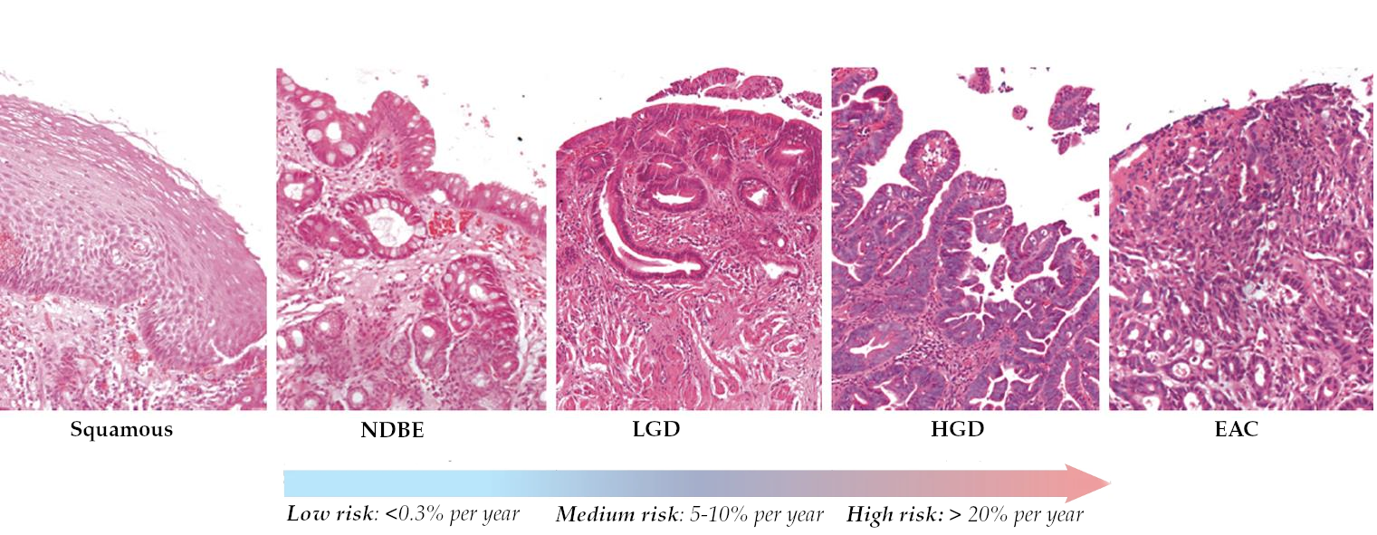
Figure 1.1: Examples of biopsies with different stages of progression. From left to right: regular squamous epithelium, non-dysplastic BE, low-grade dysplastic BE, high-grade dysplastic BE, and finally EAC (esophageal cancer).

Technical Problem

Unsupervised machine learning therefore presents itself as a promising research area. As the subfield of machine learning that does not train using any form of labeled data, it does not suffer from the high variance in labeling between different clinical professionals that characterizes the more common supervised techniques. Instead, unsupervised learning attempts to find a subset of meaningful features within the training data to accomplish its tasks, a subfield also known as representation learning Bengio et al. (2012). Not only can representation learning be used to reduce the dimensionality of the data, but it can also be used to study what features are important for making accurate predictions.

Learning Meaningful Representations with Variational Autoencoders

Analogous to how a pathologist does not use all the information observable within a biopsy to make diagnoses, but instead looks at specific features such as glands, number of cells, and the shape of the tissue, a machine learning model also does not require all the information present in the data and would benefit more from a lower-dimensional representation that only contains features useful to the diagnosis task. According to the manifold hypothesis, this set of useful features lies on a lower-dimensional space that is embedded in the entire data space, also known as a manifold. Variational Autoencoders (VAE), a generative type of deep neural network, are able to learn such a space. VAEs attempt to learn this manifold from the data following a process of compressing and decompressing the input data, such that it can be compressed and accurately reconstructed from the lower-dimensional manifold space Kingma and Welling (2013).

The great benefit of this type of modeling is that we can explore and interpret the manifold space, in which quantities such as placement or distance between data points hold semantic information. By learning to map histopathological data to such a manifold space, we can therefore model the progression of Barrett’s esophagus. For instance, the VAE may learn a latent space in which different classes of precursor lesions are spatially separated, and points from the same class form clusters. Not only would this give insight into how different stages of BE relate to each other, but such a representation would also decrease the current reliance of classification models on hand-crafted labels, which are expensive to annotate and contain a large amount of bias. Moreover, the latent space can be used to generate interpolations between different data points and different progression stages. If the model is able to capture the variation in the morphological structure of cell tissue as the disease progresses, such interpolations will result in intermediate stages of dysplasia that occur in between the four different classes most commonly used now. Such interpolations would allow us to model the progression of BE in a more continuous manner and might reveal information that was previously unknown or not used by classifiers.

Representation learning with variational autoencoders therefore seems like a promising direction for digital histopathology of BE, not only for improving the quality of supervised classification tasks, but also for its interpretability and possibility of gaining new medical insights.

Geometric Variational Autoencoders

One issue with representations learned by VAEs, however, is that they tend to severely distort relationships between points, which significantly hinders their ability to model disease progression. This is most commonly attributed to the assumption of the latent manifold as a flat Euclidean space. Because of this distortion that the Euclidean assumption creates, relationships such as distance between points tend not to reflect semantic similarities well. This greatly reduces the interpretability of the representation space, hinders potential use for unsupervised learning of classes, and reduces the usefulness for application to downstream tasks.

Recently, research has therefore attempted to solve this issue by proposing geometric variational autoencoders. These types of models use alternative, non-Euclidean topologies of the latent space, aiming to structure the manifold in a more geometrically meaningful way. Two such methods, RHVAE (Chadebec et al., 2020) and $\mathcal{S}$-VAE (Davidson et al., 2018), that subsequently assume Riemannian manifolds and hyperspherical manifolds, demonstrated promising results on image data and were expected to also extend well to a medical use case. Moreover, an extension of $\mathcal{S}$-VAE to disentangle rotation information from latent representations was proposed by Vadgama et al. (2022). The roto-equivariant group neural network at the basis of this work was earlier shown by Lafarge et al. (2020) to outperform regular VAEs on a histopathological dataset similar to this work, for example producing high-quality interpolations.

Although all the above methods have demonstrated improved performance over regular VAEs in creating a meaningful, geometrically-aware latent space with improved clustering, generation, and interpolation ability, they have not been applied to many real-life datasets yet, and the potential for medical image analysis, especially histopathological data, has been relatively unexplored. Hence, this work will apply these methods, RHVAE, $\mathcal{S}$-VAE and roto-equivariant $\mathcal{S}$-VAE , to the use case of modeling Barrett’s esophagus progression and study whether the additional geometric structuring of the VAEs’ latent space improves the models’ ability to create meaningful representations. We hypothesize that the progression of healthy tissue to Barrett’s esophagus can be modeled in such a geometrically structured latent space, therefore allowing us to take a step further towards supporting histopathological diagnosis of esophageal cancer precursor lesions.

1.1. Research Questions

This work aims to answer the following research questions.

• In what way can we geometrically structure the latent space of a VAE such that it represents a modelling of the progression of healthy tissue to Barrett’s esophagus?

• Which of the different manifold topologies, Euclidean, Riemannian or hyperspherical, lead to the best performance in terms of reconstruction quality, classifiability of latent representations and quality of generated images?

• Does the disentanglement of rotation from the learned latent representations improve performance on the aforementioned tasks?

• Can we create a non-variational spherical autoencoder that is able to generate images of comparable quality to a variational model, while retaining the benefits of autoencoder models over variational models?

1.2. Contributions

The key contributions of this work can be summarized as follows:

• We study two different instances of latent manifold topologies, a Riemannian manifold and a hyperphysical manifold, through the use of RHVAE and $\mathcal{S}$-VAE , and apply them to the novel use case of histopathological image data.

• We evaluate both quantitatively and qualitatively how these models perform in comparison to a vanilla VAE by reporting reconstruction error, downstream classification accuracy, generative sampling quality, and interpolation quality. We show that $\mathcal{S}$-VAE is able to create more meaningful representations, but is limited to a lower-dimensional latent space size.

• We also investigate KS-VAE, a rotation disentangled extension of $\mathcal{S}$-VAE , and show how it can be used to improve structuring of the latent space by an increased amount over the non-disentangled models.

• We propose to use non-variational hyperspherical autoencoders as an alternative to $\mathcal{S}$-VAE in higher dimensions, and show its increased stability and improved reconstruction quality over variational spherical models.

• We take a first step towards the novel use of spherical autoencoders as a generative model, by introducing a custom loss function called spread loss. We show that $\mathcal{S}$-AE can be used to generate images comparable in quality to those of a variational model, while still retaining the qualities described above.

1.3. Outline

This work consists of a total of five further sections. The first of these sections, Section 2, provides background for this study through some required clinical knowledge, a literature review on the field of representation learning, a more in-depth motivation of geometrically-structured latent spaces, and related work that has been done in this field. Secondly, Section 3 will provide the technical details on the models used in this work. Next, the data and experimental setup will be discussed in Section 4, after which we report the results in Section 5. Finally, Section 6 concludes this work with an analysis of the results and suggestions for future work.

Section 2. Background

The following section will provide the reader with a background for this research. First of all, Subsection 2.1 will give a short introduction to Barrett’s Esophagus from a clinical point of view. We believe that understanding what the progression of Barrett’s Esophagus looks like and following along with how a histopathologist makes their diagnoses, will greatly help in conveying what we eventually want our model to do, which is learning what features are important and using this knowledge to model the progression of the disease. Subsection 2.2 will therefore focus on developments in the field of representation learning, which is concerned with learning meaningful features from high-dimensional data. Here we will also introduce manifold learning through variational autoencoders. Finally, Subsection 2.3 will introduce geometrically-aware VAEs. We will explain why the lack of structuring in the latent space of regular autoencoder models can distort relationships between different data classes and propose to solve this issue by providing additional geometric structure to the latent space.

2.1. Clinical Background: Barrett’s Esophagus

Esophageal adenocarcinoma (EAC), one of the most common subtypes of esophageal cancer, is an aggressive form of cancer with a poor prognosis. Only around 20% of diagnosed patients survive past five years after their diagnosis. When it is discovered at an early stage however, this rate can increase to around 45% He et al. (2020). It is therefore essential that EAC is diagnosed early on in the disease progression. Currently, research into early-stage diagnosis has determined only one independent precursor lesion to esophageal adenocarcinoma: Barrett’s Esophagus (BE). Barrett’s esophagus is a condition that is characterized by a change of the cell tissue lining the esophagus (squamous epithelial cells) to cells that closely resemble those ordinarily lining the stomach (metaplastic columnar mucosa cells).

Because of the importance of early diagnosis, all patients diagnosed with BE are accepted for endoscopic surveillance. The endoscopic screening procedure consists of taking multiple biopsies from the esophagus lining, staining these with hematoxylin and eosin (H&E) coloring, and digitalizing these through a dedicated scanner Van der Wel et al. (2016). A histopathologist then examines these digital biopsies under a microscope and determines the severity of the dysplasia. Labeling the progression is done in accordance with the Vienna criteria, which were developed to reduce diagnostic differences between different practitioners. It should be noted that although these criteria helped standardize labeling systems, the interobserver variability for BE diagnoses is still very high van der Wel et al. (2020). Following the criteria, Barrett’s esophagus is subdivided into three increasingly more severe classes of dysplasia: Non-Dysplastic Barrett’s Esophagus (NDBE), Low-Grade Dysplasia (LGD), and High-Grade Dysplasia (HGD), or into a fourth indefinite class when diagnoses are highly uncertain Van der Wel et al. (2016). Average progression rates of BE into EAC increase with the severity of the dysplasia in BE. While patients with non-dysplastic BE only have an annual conversion rate of less than 0.3%, that rate increases up to 10% for low-grade dysplasia and to more than 20% for high-grade dysplasia. See also Figure 1.1. Treatment plans therefore are highly dependent on correct classifications of the different stages of BE.

Van der Wel et al. cite five general features that allow pathologists to make accurate classifications. In order of importance, these are clonality, surface maturation, the architecture of the glandular structures, cytonuclear abnormalities, and inflammation. For example, abrupt transitions between nuclear features (clonality) are an important marker for dysplastic BE, as well as decreased surface maturation. For high-grade dysplasia specifically, the number of nuclei also increases, and they tend to form more complex growth patterns. Conversely, in non-dysplastic BE, the surface maturation and architecture remain intact, but glands can start to appear more uniform or rounded as compared to regular squamous epithelium Ong et al. (2010).

The disease progression is therefore characterized by changes in tissue morphology, which we want a machine-learning model to be able to capture. The following subsection will therefore give an introduction to the field of representation learning and motivate the choice of manifold learning through geometric variational autoencoders for modeling BE disease progression. Through this approach, it becomes possible to avoid the need for expensive and high-variance annotations made by pathologists, as mentioned earlier.

2.2. Technical Background: Representation Learning

Machine learning has become increasingly successful at a multitude of tasks over the past few years. A part of that success can be attributed to developments in the field of representation learning, or feature learning, which attempts to learn meaningful representations or features of data (Bengio et al., 2012). It is often hypothesized that different data representations can entangle different explanatory factors within the data, so choosing a representation that hides unimportant -or conversely highlights important factors allows deep learning methods to more easily make classifications. A well-known example of representation learning is the embedding of text into word vectors through models such as word2vec (Mikolov et al., 2013), which has become the standard representation of words for downstream natural language processing tasks and has greatly improved the ability of NLP models to relate and reason about language. More recently, models such as BERT (Devlin et al., 2018) and GPT (Radford et al., 2018) have also learned rich distributed representations from a language modeling task and have achieved state-of-the-art results on numerous NLP problems. Outside of the field of NLP, representation learning has been applied to many real-world data applications, such as images, speech signals, video, and bioinformatics, not only to learn richer representations of the data but also to reduce its often high dimensionality (Van Der Maaten et al., 2009).

2.2.1.  Manifold Learning

While classic examples of dimensionality reduction, such as Principal Component Analysis (PCA) (Wold et al., 1987), or Multi-Dimensional Scaling (MDS) (Cox and Cox, 2008), are able to learn linear embeddings, more recent developments have focused on methods of non-linear dimensionality reduction, also known as manifold learning. This increasingly more popular subfield is based on the hypothesis that probability mass concentrates near regions that have a much smaller dimensionality than the space in which the original observed data lies (Cayton, 2005). The data can therefore be said to lie on a low-dimensional manifold, a topological space that locally resembles Euclidean space, embedded in a higher-dimensional space. Such a manifold space reflects variations in the input data in its intrinsic coordinate system, i.e., quantities such as location and pairwise distances represent relationships between input data points. Manifold learning thus aims to learn the aforesaid data-supporting space, resulting in a representation that models relationships between data points in an inherently more geometric way as compared to other subfields of representation learning (Fefferman et al., 2016).

Intuitively, this hypothesis also has a basis in real-life concepts from psychology and biology. Taking the task of facial recognition as an example, it is generally assumed that a human perceiver has a priori access to a representation of stimuli in terms of some perceptually meaningful features that can support the relevant classification. High-dimensional, raw input signals are mapped to these features by some complex function, which is learned naturally by humans (Tenenbaum, 1997). Comparingly, machine learning models also receive high-dimensional input data: if for instance our facial images are grayscale and of size $28\times 28$, then that means that they lie in a $784$-dimensional observation space, with a total of $256^{7}84$ possible images. However, only a very small portion of this set of possible images corresponds to a meaningful, naturally-occurring representation of a face. These perceptually meaningful images can therefore be said to lie on a much lower-dimensional manifold, to which a machine learning model can learn a mapping. This also means that small variations in the naturally-occurring input images, such as changes in light, rotation, or texture, can be mapped to corresponding changes in the lower-dimensional manifold. Learning this structure of the manifold would therefore allow the model to reason more effectively about the data (Fefferman et al., 2016).

The Non-Parametric Approach: Kernel Methods

Some classic examples of manifold learning fall into the family of kernel methods, or spectral methods, which includes notable examples such as Isomap (Tenenbaum et al., 2000), Locally Linear Embedding (LLE) (Roweis and Saul, 2000) and Diffusion Maps (Coifman et al., 2005). These methods have in common that they attempt to approximate the manifold by a local neighborhood graph, creating a lower-dimensional representation that preserves some of the underlying geometry between data points; for example, through pairwise geodesic distances in the case of Isomap, through linearity of neighborhoods in the case of LLE and through heat kernels in the case of diffusion maps.

Kernel methods have been used for manifold learning and dimensionality reduction in a variety of medical tasks. Souvenir and Pless (2005) for instance, apply isomap to MRI scans of heart and lungs and theorize that the manifold learned through isomap is able to parametrize the deformations of heart shape caused by patient’s breathing (Souvenir and Pless, 2005), therefore allowing for a lower-dimensional representation that captures meaningful morphological relationships between different images. Similarly, Piella (2014) applies kernel methods to the task of multimodal image registration and uses diffusion maps to map a dataset of brain scans to a manifold that reflects its geometry uniformly across modalities. Finding related images can then be solved by computing the similarity between them through a simple Euclidean distance metric (Piella, 2014).

The Parametric Approach: Autoencoders

While the ability of kernel methods to preserve an underlying geometric structure enables them to learn efficient and meaningful low-dimensional data representations, they suffer from a major drawback: they are only able to map the input data to a fixed set of coordinates, making it impossible to naturally embed any new data point that was not used for fitting the model. This greatly restricts the use of these types of models. A manifold learning technique that does not suffer from this problem is the Autoencoder (AE) (Rumelhart et al., 1986). In contrast to kernel methods, AEs learn a parametric function, which allows them to both perform inverse mappings and embed out-of-sample points.

Autoencoders are a type of neural network that imposes a bottleneck on the network architecture, which has the effect of enforcing a compression on the input data. Specifically, the architecture consists of an encoder part which encodes the input data into a lower-dimensional manifold space, also known as the latent space, and a decoder, which learns to most accurately reconstruct the original input data from these latent vectors learned by the encoder. In this way, the quality of the reconstruction is directly influenced by the quality of the learned latent representation, and it becomes possible to visually assess the quality of the representation by observing the quality of the reconstructed output.

Moreover, a more recent variant of the autoencoder model, the Variational Autoencoder (VAE), instead has the encoder learn to output parameters for a probability distribution characterizing each input data point from which latent vectors can then be sampled (Kingma and Welling, 2013; Rezende et al., 2014). Because the latent manifold space of a VAE is continuous, it becomes possible to not only learn accurate reconstructions of the input, but also to generate new unseen data points based on the input data. Moreover, by treating the knowledge within the learned representation as a hypothesis, it becomes possible to inspect reconstructions, generations, and visualizations of the latent space to assist in understanding what the model has learned and whether it corresponds to our own understanding of the world. It may even be used to learn of new structure within the data that is not apparent in the original form of the input. Such ability has great appeal for biomedical imaging applications and can in particular be of great help in understanding the complex problem of the histological diagnosis of disease.

Not only can VAEs be used to generate new data points in case of sparse available datasets, which is often the case in medicine, but there are numerous other benefits to the use of these models for a histopathological use case. First of all, they may learn a latent representation in which different classes of precursor lesions are spatially separated and points from the same class form clusters (Wang and Wang, 2019; Zeune et al., 2020). Finding such a representation would decrease the current reliance of classification models on hand-crafted labels, which are expensive to annotate and can contain a large amount of bias (van der Wel et al., 2020). Secondly, it becomes possible to generate interpolations between different data points and different classes (Thomas, 2022; Wang and Wang, 2019). By visually inspecting these interpolations, we can assess if the model is able to realistically capture the variation in morphological structure of cell tissue as it transforms into a malignant state. Finally, if the latter is the case, we can also perform extrapolation to unseen states of the data, which might reveal information about the progression that was previously unknown.

However, despite these properties, AEs often fail to accurately recover the geometry present in the data. This not only restricts their desirability to perform exploratory data analysis, but can also lead to poor-quality reconstructions over certain regions in the learned latent space where data is sparse, decreasing the quality of interpolations and generations. Previous research has often seen that the underlying shape of the manifold on which the input data lies is not preserved when mapping to the latent space (Duque et al., 2020). This has as a consequence that some of the underlying relations between data points, such as cell deformations and morphological characteristics of tissue in our current use case, are lost, which leads to less rich representations. Ideally, we would require a model that can preserve these properties when modeling the latent manifold space, but not in the limited way of creating neighborhood graphs like in the non-parametric approach.

2.3. Geometric Variational Autoencoders

Recent research has therefore looked into solving the distortion issues of VAEs, focusing on modeling the latent space in a non-Euclidean way and instead exploring alternative manifold topologies. Before we discuss the details of these geometric VAEs however, it is important to understand the reasons behind the distortion of the latent space and how the Euclidean assumption relates to this problem.

The Distortion of the Latent Space

Formally, a VAE is a neural network architecture that aims at learning a parameterized probability distribution $p_{\theta}$ describing the input data $x$’s true distribution $P(x)$. To do so, we assume that the input data can be characterized by lower-dimensional latent vectors $\mathbf{z}$. The marginal likelihood can then be written as

$$p_{\theta}(\mathbf{x})=\int p_{\theta}(\mathbf{x}|\mathbf{z})q(\mathbf{z})d\mathbf{z},$$ (2.1)

where $q(\mathbf{z})$ is a prior distribution over the latent variables, that in case of the vanilla VAE is chosen as a standard normal distribution $q(\mathbf{z})=\mathcal{N}\left(\mathbf{z}\mid\mathbf{0},\mathbf{I}_{\mathbf{d}}\right)$.

The consequence of assuming a Gaussian prior is that this distribution tends to move clusters closer together in the latent space (Yang et al., 2018). The architecture of the VAE is made to minimize the distance between the prior and posterior distribution, so learned latent variables can be forced to show structure based on the Gaussian prior, even if that structure was not originally present in the data. This can cause a distortion in the latent space that affects clustering, interpolation and more. Take for example the curved manifold of the observed input space shown on the right of Fig 2.1(a) and its learned latent representation on the left. If we want to interpolate between two points by calculating the shortest distance between them, a natural choice of interpolant would be the green curve, as it follows the shape of the observed space and creates a well-informed path over the manifold. However, if we calculate the shortest distance between these same points in the latent space, we actually end up calculating a path that not only corresponds to a longer path in the observed space, but also crosses through areas containing points of a different class and areas where no data or information is present at all, leading to an interpolation of lower quality than the green curve.

Similarly, in figure 2.1(b), we observe the latent representation of two digits from the MNIST dataset learned by a vanilla VAE Deng (2012). Unintuitively, under this representation, points B and C are closer in distance than points A and B, even though the latter belong to the same class. However, following the same logic as above, we can assume that the real high-dimensional input data actually lives in a manifold where the relations between points are in fact meaningful, it is just due to the distortion of the latent space that these relations cannot become apparent.

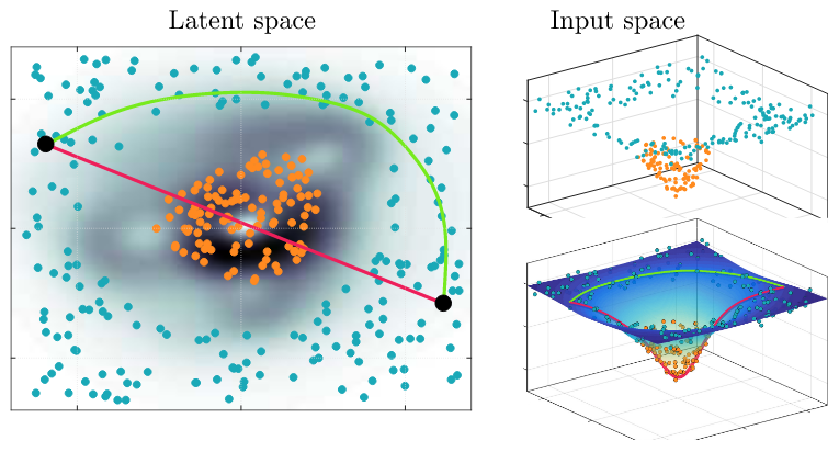
(a)

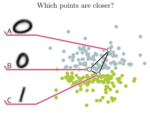
(b)

Figure 2.1: Example of how the distortion of latent space influences interpolation paths and clustering.

Although the above is just a toy example, it becomes apparent that the distortion of the latent space influences interpolations, clustering and visual interpretability of the representations that are learned and that this impact becomes more significant with the magnitude of relative distortion present; the greater curvature there exists in the original input data, the more distorted the relationship between points in the latent space becomes. In the case of medical data, which is often high-dimensional and complex, finding a more geometrically relevant representation therefore becomes especially important (Krioukov et al., 2010). If we can learn a latent representation that is more geometrically correct, this would improve interpolations, clusterings, latent probability distributions, sampling algorithms, interpretability and more. The question then becomes in what way we can construct such a geometrically meaningful space.

Challenging the Euclidean Assumption

One popular direction of research has therefore put the assumption of Euclidean latent space up for debate. Natural image data in general has been shown to possess a strong non-Euclidean latent structure, because it is said to live on a “natural image manifold” of which an example was given earlier Skopek et al. (2019), and also medical imaging specifically has been named as a domain that is naturally non-Euclidean Bronstein et al. (2017). Assuming a non-Euclidean topology of the latent space therefore seems especially interesting in the context of the histopathological problem. Not only have Euclidean topologies shown to cause problems when learning manifolds with different topologies (Falorsi et al., 2018), but they are also not invariant arithmetically, which causes any deformations of the latent space to also lead to changes in the estimated data density. This leads to the identifiability problem commonly observed in generative models, which entails that many configurations of the latent space can explain the observed data equally well (Bishop and Nasrabadi, 2006; Hauberg, 2018). The identifiability problem forms a significant drawback in the interpretability of the latent space, its robustness, and its potential to reveal unknown structures in the data. Alternatives to the Euclidean topology are therefore urgently needed.

2.3.1.  The Latent Space as General Riemannian Manifold

One commonly proposed method is to endow the latent space with a Riemannian metric, making it possible to define geometric properties in the input space rather than the distorted latent manifold space. As this latent space can be arbitrarily deformed following the aforementioned infidelity problem, the notion of distance here would be unreliable for defining relationships between points. A solution would therefore be to not define distances in the distorted latent space, but instead in the original input space. Because VAEs in practice span a manifold embedded in the original input space, it becomes possible to measure distances along the shape of this manifold by endowing it with a Riemannian metric, therefore making it a Riemannian manifold space (Tosi et al., 2014; Arvanitidis et al., 2017; Chen et al., 2018; Shao et al., 2018). Riemannian geometry, unlike Euclidean geometry, considers space to be curved. A Riemannian metric can be thought of as an extra structure or shape on a manifold that allows for locally defining properties such as angles, distances, and volume. (Riemann, 1868) Endowing the latent space with such a metric makes it possible to ensure that distances between points in the latent space are identifiable, even if the coordinates themselves are not. We can thereby bypass the problem of distortion of the latent space.

This idea has recently proven its potential for a multitude of problems. Arvanitidis et al. (2017) show that using a Riemannian distance metric significantly improves clustering using K-means on the MNIST dataset and that the visual quality of interpolations substantially improves. These results are independently confirmed by Chen et al. (2018) and Yang et al. (2018). Furthermore, Detlefsen et al. (2022) apply the method to one-hot encoded protein sequences and find that they are able to preserve the phylogenetic tree-structure originally present in the data, as well as create natural interpolations that follow along this tree-shaped manifold. Finally, Beik-Mohammadi et al. (2021) apply it to capturing relevant motion patterns in robotics and are capable of efficiently planning robot motions based on human demonstrations as well as designing new motion patterns that were not observed originally. Both of these applications suggest that the Riemannian manifold representation succeeds in capturing a morphological quality present in the data; motion-based in the case of robotics and an evolutionary morphology in the case of proteins. Such a method seems highly suitable to investigate for a histopathological use case, as we would ideally want to create representations that capture the morphology of cell tissue from healthy to cancerous.

Nevertheless, these models all suffer from one common issue: obtaining a Riemannian metric involves the computation of a Jacobian, which requires solving a system of ordinary differential equations. Systems like these do not always have a closed-form solution and are hard to evaluate with standard deep-learning frameworks. Solutions approximating the Jacobian, such as finite difference methods, introduce bias into the network, while relying on automatic differentiation is computationally costly. This makes the utility of the proposed method especially limited for high-dimensional datasets such as those containing images and even more so for the high-resolution biopsy scans used in histopathology. Chadebec et al. (2020) therefore propose their model RHVAE (Riemannian Hamiltonian Variational Autoencoder), which instead of computing the Riemannian metric numerically, learns it from the data. Not only does this avoid the need for computing a Jacobian, but it also provides more flexibility since no prior knowledge about the structure of the manifold is imposed on the model. Besides showing improved quality of interpolations on MNIST and FashionMNIST, the authors also apply their method to a biomedical use case in a follow-up study (Chadebec et al., 2021). There, they use RHVAE to augment a small-scale dataset of MRI scans, containing healthy scans and scans of patients with Alzheimer’s disease and show that training a CNN on the newly generated images improves overall classification performance.

2.3.2.  The Latent Space as Manifold of Constant Curvature

The approaches above intend to solve the problem of the distorted latent space by assuming it to be a Riemannian manifold instead of a Euclidean space and accomplish this by endowing it with a Riemannian metric. However, as discussed, many of these approaches are not computationally feasible due to a lack of closed-form solutions. An alternative to general Riemannian manifolds is therefore the use of manifolds of constant sectional curvature Skopek et al. (2019); Bachmann et al. (2020); Gu et al. (2018). Constant curvature manifolds are one of the only types of Riemannian manifolds for which closed-form solutions to quantities such as distances and exponential maps exist. They consist of three different types, namely elliptic (positive curvature), Euclidean (zero curvature), or hyperbolic (negative curvature). In cases where Euclidean geometry fails to accurately represent the data, the hyperbolic and spherical spaces can possibly provide a better inductive bias for the respective data. For instance, the hyperbolic space can be thought of as a continuous tree. Intuitively, it would seem that a hyperbolic structuring of the latent space could therefore be beneficial for hierarchical or tree-structured data, such as text or protein sequences. VAE models that structure the latent space in a hyperbolic way have indeed seen improved results on tasks such as the creation of word embeddings, and possess the ability to naturally exploit the semantic structure present in natural language data Tifrea et al. (2018); Nagano et al. (2019). Conversely, the elliptic space can be thought of as a sphere and as such, provides benefits for modeling cyclical or spherical data. Examples of naturally spherical data include meshes, radiation waves, and 3D scans in medical imaging. Moreover, spherical spaces have also been shown to be better fit any form of normalized data, which is a common preprocessing step in modern deep-learning problems Davidson et al. (2018).

Examples of models utilizing a spherical latent space are Batmanghelich et al. (2016) and Xu and Durrett (2018), who apply it to natural language processing and Davidson et al. (2018) who use it on image data. In this work, Davidson et al. replace the Gaussian prior and posterior of the vanilla VAE to a uniform distribution and a von Mises–Fisher (vMF) distribution respectively, therefore creating a spherical latent space over which embedded points are spread uniformly. Using the MNIST image dataset, they show that $\mathcal{S}$-VAE has improved quality of clusterings and interpolations over a vanilla VAE, and even has the ability to generalize to non-spherical data manifolds.

2.3.3.  Equivariant Hyperspherical VAEs

One downside of the above geometric models and VAEs in general is that they may encode information present in the data that is not actually relevant to the representation. An example of this for medical images specifically is orientation. Biopsies can be scanned in any arbitrary orientation, so the information about rotation is not actually a relevant component of the encoded representation and can possibly be a disrupting factor in downstream tasks. Lafarge et al. (2020) therefore propose a rotation-equivariant VAE model ($SE$(2)-VAE). They extend the vanilla convolutional VAE to a group-convolutional neural network Cohen and Welling (2016a), making the model invariant to arbitrary rotations. This allows the VAE to learn both a representation vector and an orientation of an input image. Such an equivariant network can therefore disentangle the rotation from the rest of the latent representation. Lafarge et al. show that this is a very useful property for representation learning of histopathological image data, improving the quality of generated image interpolations over the vanilla VAE model. It is worth noting that there is not much research on representation learning for histopathological image data specifically, so the insights provided by Lafarge et al. can prove valuable to the current work. However, as the model still assumes a Euclidean latent space, it suffers from the same distortion issue present in the original VAE.

Therefore, Vadgama et al. (2022) more recently combined the methods of Lafarge et al. and the hyperspherical model of Davidson et al. to create a VAE that features a hyperspherical latent space, while also being an orientation-disentangled group-convolutional network. They show that such a model is able to correctly learn orientations of MNIST images and that the model outperforms both vanilla autoencoders and the non-equivariant hyperspherical $\mathcal{S}$-VAE in terms of minimizing loss. Since the group-convolutional VAE of Lafarge et al. was shown to produce good results on a histopathological image dataset, it would be interesting to see how this translates to the model of Vadgama et al..

$\thicksim$

This section described three different types of geometric variational autoencoders, which all relate to medical imaging in some way. For the Riemannian VAEs, the model of Chadebec et al. (RHVAE) showed promising results on brain scans. Moreover, for the constant curvature models, the hyperspherical manifold type, such as the $\mathcal{S}$-VAE model used in Davidson et al., seemed the most applicable to image data. An extension of the hyperspherical model that disentangles orientation (KS-VAE) was proposed by Vadgama et al. and the equivariant VAE model at the basis of this method, originally proposed by Lafarge et al., was shown to achieve high-quality interpolations. We will therefore compare the RHVAE, $\mathcal{S}$-VAE , and KS-VAE models and apply them to the novel use case of histopathological image data.

Section 3. Methodology

This section explains the theoretical details of the models used in the experiments. These are the regular vanilla variational autoencoder (VAE), the Riemannian Hamiltonian variational autoencoder (RH-VAE), the spherical variational autoencoder ($\mathcal{S}$-VAE ) and the roto-equivariant Variational Auto-Encoder (KS-VAE).

3.1. Variational Autoencoder

At the basis of all models used in this work lies the autoencoder model. The general framework of an autoencoder consists of two neural networks: an encoder that encodes an input image $x$ into a lower-dimensional latent representation $z$, and a decoder that decodes the latent representation into a reconstruction $\hat{x}$, with the aim of minimizing the error between the original image and its reconstruction. The Variational Autoencoder (VAE) (Kingma and Welling, 2013) is a generative version of the original autoencoder, that instead of learning the latent representation $z$ directly, learns a distribution describing each data point, from which the latent representation is sampled (see Figure 3.1). The aim of the VAE is therefore to learn a parameterized probability distribution $p_{\theta}$ describing the input data $x$’s true distribution $P(x)$. To do so, we assume that the input data can be characterized by a lower-dimensional latent distribution $z$. The marginal likelihood can then be written as

$$p_{\theta}(x)=\int p_{\theta}(x|z)q_{prior}(z)dz$$ (3.1)

where $q_{prior}(z)dz$ is a prior distribution over the latent variables, that in case of the vanilla VAE is chosen as a standard normal Gaussian distribution. Unfortunately, computing $p_{\theta}(x)$ involves the posterior $p_{\theta}(z|x)$, which is computationally expensive and often intractable. We therefore introduce an approximation $q_{\phi}(z|x)$ of the true posterior, which is computed by a neural network: the encoder. We can then train a variational autoencoder, consisting of the encoder, which computes the approximate posterior and the decoder, which computes the conditional likelihood $p_{\theta}(x|z)$.

Within the variational autoencoder framework, the encoder and decoder are optimized in a joint setting. To find the posterior distribution $q_{\phi}(z|x)$ that best approximates the true posterior $p_{\theta}(z|x)$, we can use the Kullback-Leibler divergence, which measures the difference between two probability distributions. Ideally, we would want to minimize this term, which is given by

$$\text{KL}(q_{\bm{\mathbf{\phi}}}(\bm{\mathbf{z}}\mid\bm{\mathbf{x}})\,\,||\,\,p_{\bm{\mathbf{\theta}}}(\bm{\mathbf{z}}\mid\bm{\mathbf{x}})) =\mathbb{E}_{q_{\phi}}\big{[}\log q_{\phi}(\mathbf{z})\big{]}-\mathbb{E}_{q_{\phi}}\big{[}\log p_{\theta}(\mathbf{z}|\mathbf{x})\big{]}$$ (3.2)

$$=\mathbb{E}_{q_{\phi}}\big{[}\log q_{\phi}(\mathbf{z})\big{]}-\mathbb{E}_{q_{\phi}}\bigg{[}\log\frac{p_{\theta}(\mathbf{x},\mathbf{z})}{p_{\theta}(\mathbf{x})}\bigg{]}$$ (3.3)

$$=\mathbb{E}_{q_{\phi}}\big{[}\log q_{\phi}(\mathbf{z})\big{]}-\mathbb{E}_{q_{\phi}}\big{[}\log p_{\theta}(\mathbf{x},\mathbf{z})-\log p_{\theta}(\mathbf{x})\big{]}$$ (3.4)

$$=\mathbb{E}_{q_{\phi}}\big{[}\log q_{\phi}(\mathbf{z})-\log p_{\theta}(\mathbf{x},\mathbf{z})\big{]}+\mathbb{E}_{q_{\phi}}\big{[}\log p_{\theta}(\mathbf{x})\big{]}$$ (3.5)

$$=\mathbb{E}_{q_{\phi}}\big{[}\log q_{\phi}(\mathbf{z})-\log p_{\theta}(\mathbf{x},\mathbf{z})\big{]}+\underbrace{\log p_{\theta}(\mathbf{x})}_{\text{intractable}}.$$ (3.6)

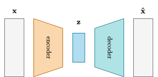
(a)

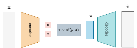
(b)

Figure 3.1: Schematic view of autoencoder and variational autoencoder architectures. The encoder either learns to map the input vector $\mathbf{x}$ to a latent vector $\mathbf{z}$ directly (AE), or learns the parameters of a distribution describing $\mathbf{x}$, from which $\mathbf{z}$ is then sampled (VAE). The decoder in both cases learns to most accurately reconstruct the original input ($\mathbf{\hat{x}}$) from $\mathbf{z}$.

However, as can be seen when we rewrite the equation, we still have the intractable evidence term $\log p_{\theta}(\mathbf{x})$. We therefore introduce a lower bound of the log-likelihood using Jensen’s inequality.

$$\log p_{\theta}(x) =\log\int_{\mathbf{z}}p_{\theta}(\mathbf{x},\mathbf{z})$$ (3.7)

$$=\log\int_{\mathbf{z}}p_{\theta}(\mathbf{x},\mathbf{z})\frac{q_{\phi}(\mathbf{z})}{q_{\phi}(\mathbf{z})}$$ (3.8)

$$=\log\left(\mathbb{E}_{q_{\phi}}\left[\frac{p_{\theta}(\mathbf{x},\mathbf{z})}{q_{\phi}(\mathbf{z})}\right]\right)$$ (3.9)

$$\geq\underbrace{\mathbb{E}_{q_{\phi}}[\log p_{\theta}(\mathbf{x},\mathbf{z})]-\mathbb{E}_{q_{\phi}}[\log q_{\phi}(\mathbf{z})]}_{\text{ELBO}}$$ (3.10)

This lower bound is called the Evidence Lower BOund (ELBO) (Kingma and Welling, 2013). Because the evidence is a constant, maximizing the ELBO amounts to minimizing the KL divergence. The ELBO therefore forms the key to variational inference: instead of finding our optimal distribution q by minimizing the KL divergence, requiring us to calculate the intractable evidence term, we find it by maximizing ELBO, which is a tractable operation. We can therefore use the ELBO as our model’s loss function. To arrive at our final loss function, we rearrange the ELBO term into the following expression

ELBO $$=\mathbb{E}_{q_{\phi}}[\log p_{\theta}(\mathbf{x},\mathbf{z})]-\mathbb{E}_{q_{\phi}}[\log q_{\phi}(\mathbf{z})]$$ (3.11)

$$=\mathbb{E}_{q_{\phi}}[\log p_{\theta}(\mathbf{x},\mathbf{z})-\log q_{\phi}(\mathbf{z})]$$ (3.12)

$$=\mathbb{E}_{q_{\phi}}[\log p_{\theta}(\mathbf{x}|\mathbf{z})+\log p_{\theta}(\mathbf{z})-\log q_{\phi}(\mathbf{z})]$$ (3.13)

$$=-\mathbb{E}_{q_{\phi}}[\log p_{\theta}(\mathbf{x}|\mathbf{z})-\mathbb{E}_{q_{\phi}}[\log p_{\theta}(\mathbf{z})-\log q_{\phi}(\mathbf{z})]$$ (3.14)

$$=-\mathbb{E}_{q_{\phi}}[\log p_{\theta}(\mathbf{x}|\mathbf{z})]-\text{KL}\left(q_{\bm{\mathbf{\phi}}}\left(\bm{\mathbf{z}}\mid\bm{\mathbf{x}})\,\,||\,\,p_{\bm{\mathbf{\theta}}}(\bm{\mathbf{z}}\right)\right),$$ (3.15)

which consists of a regularization term $\mathbb{E}_{q_{\phi}}[\log p_{\theta}(\mathbf{x}|\mathbf{z})]$ and a KL divergence term $\text{KL}\left(q_{\bm{\mathbf{\phi}}}\left(\bm{\mathbf{z}}\mid\bm{\mathbf{x}})\,\,||\,\,p_{\bm{\mathbf{\theta}}}(\bm{\mathbf{z}}\right)\right)$. The expectation term is also called the reconstruction loss. It pushes the model to most accurately reconstruct an image from its encoded latent representation, such that the difference between decoding a sampled latent vector from the learned distribution is as small as possible. Meanwhile, the KL divergence term is also called the regularization loss, as it pushes the approximate posterior to more closely resemble the prior distribution. When choosing a normal Gaussian distribution for both the prior and approximate posterior, as is the standard for VAEs, the prior enforces the posterior probability mass to have spread like a Gaussian, therefore adding a form of regularization to the model. Moreover, for a Gaussian prior and posterior, the KL term reduces to a closed-form formula, making computations more efficient.

Now, all that remains is to solve the problem of the random sampling operation from $\mathbf{z}$ not being differentiable. Kingma and Welling propose to solve this by using the reparameterization trick, which suggests that instead of sampling $\mathbf{z}$ directly, some noise $\epsilon$ is sampled from a unit Gaussian distribution. We can then add the learned mean parameter $\mu$ to this noise term and multiply it by the variance $\sigma$ to arrive at a mean and variance as would have been directly sampled from the latent distribution, while still allowing for backpropagation through the neural network.

3.2. Riemannian Variational Autoencoder

As discussed in Section 2.3, the vanilla variational autoencoder suffers from a distortion in the latent space as a consequence of the Euclidean manifold assumption and Gaussian prior, which makes geometric notions such as distance unreliable in this space. One way of remedying this problem is to use metrics defined in the non-distorted input space instead, and mapping them to the manifold space. Such a mapping is possible by endowing the manifold with a Riemannian metric. A model that not only does this, but also learns a fitting metric from the input data, is the Riemannian Hamiltonian VAE. These qualities make it a promising technique for accurately representing relationships between points and modelling BE progression.

The following section describes the details of RHVAE. Before this can be discussed however, it is important to give the reader a short overview of the basics of Riemannian geometry.

3.2.1.  Basics of Riemannian Geometry

As discussed earlier, a real, smooth manifold is a space that is locally similar to a linear space. Riemannian geometry allows for defining notions of angles, distances, and volume on such spaces by endowing the manifold with a Riemannian Metric. The manifold can then be considered as a Riemannian manifold. We define an $m$-dimensional Riemannian manifold embedded in an ambient Euclidean space $\mathcal{X}=\mathbf{R}^{d}$ and endowed with a Riemannian metric $\mathbf{G}\triangleq(\mathbf{G}_{\mathbf{x}})_{\mathbf{x}\in\mathcal{M}}$ to be a smooth curved space $(\mathcal{M},G)$. For every point on the manifold $\mathcal{M}$, there exists a tangent vector $\mathbf{v}\in\mathcal{X}$ that is tangent to $\mathcal{M}$ at $\mathbf{x}$ iff there exists a smooth curve $\gamma:[0,1]\mapsto\mathcal{M}$ such that $\gamma(0)=\mathbf{x}$ and $\dot{\gamma}(0)=\mathbf{v}$. The velocities of all such curves through $\mathbf{x}$ form the tangent space $\mathcal{T}_{\mathbf{x}}\mathcal{M}=\{\dot{\gamma}(0)\,|\,\gamma:\mathbf{R}\mapsto\mathcal{M}\text{ is smooth around $0$ and }\gamma(0)=\mathbf{x}\}$, which has the same dimensionality as the manifold. The tangent space can be viewed as the collection of all the different ways in which the points on the manifold can be passed.

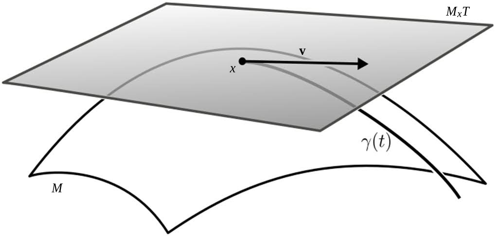
Figure 3.2: Schematic example of a 2-D manifold $\mathcal{M}$ and its tangent space $\mathcal{M}_{x}\mathcal{T}$ at point $x$. The geodesic $\gamma(t)$ starts at $x$ and goes in the direction $\mathbf{v}$.

The Riemannian metric $G(\cdot)$ then equips each point $\mathbf{x}$ on the manifold with an inner product in the tangent space $\mathcal{T}_{\mathbf{x}}\mathcal{M}$, e.g. $\langle\mathbf{u},\mathbf{v}\rangle_{x}=\mathbf{u}^{T}\mathbf{G}_{\mathbf{x}}\mathbf{v}$. This induces a norm $\|\mathbf{u}\|_{\mathbf{x}}\,,\forall\mathbf{u}\in\mathcal{T}_{\mathbf{x}}\mathcal{M}$ locally defining the geometry of the manifold. Given these local notions, we can not only compute local angles, lengths, and areas, but also derive global quantities by integrating over local properties. We can thus compute the length of any curve on the manifold $\gamma:[0,1]\rightarrow\mathcal{M}$, with $\gamma(0)=\mathbf{x}$ and $\gamma(1)=\mathbf{y}$ as the integral of its speed: $\ell(\gamma)=\int_{0}^{1}\|\dot{\gamma}(t)\|_{\gamma(t)}dt$. The notion of length leads to a natural notion of distance by taking the infimum over all lengths of such curves, giving the gobal Riemannian distance on $\mathcal{M}$, $d(\mathbf{x},\mathbf{y})=\inf_{\gamma}\ell(\gamma)$. The constant speed-length that minimizes the distance of a curve between two points is called a geodesic on $\mathcal{M}$. VAEs can generate images along such a geodesic path, providing a more geometry-aware alternative to the vanilla VAE’s linear interpolations.

3.2.2.  Riemannian Hamiltonian Variational Autoencoder

Chadebec et al. propose the Riemannian Hamiltonian VAE (RHVAE), which assumes the latent space to be structured as a Riemannian manifold $\mathcal{M}=\left(\mathbb{R}^{d},\mathbf{G}\right)$ with $\mathbf{G}$ being the Riemannian metric, as described above. RHVAE attempts to exploit this assumed Riemannian structuring by introducing two main extensions of the vanilla VAE. First, to replace the regular Gaussian posterior distribution with a geometrically-informed posterior through the use of Riemannian Hamiltonian dynamics. Secondly, to find an appropriate Riemannian metric for this space, by learning it with a neural network.

Learning the Riemannian Metric

As mentioned in section 2.3.1, while the choice of Riemannian metric is crucial to defining the manifold space, the computation of many proposed metrics involves the Jacobian, which is difficult and expensive to compute. In the RHVAE framework, the metric is therefore proposed to be learned directly from the data. This parameterized metric is defined as follows

$$\mathbf{G}^{-1}(z)=\sum_{i=1}^{N}L_{\psi_{i}}L_{\psi_{i}}^{\top}\exp\left(-\frac{\left\|z-c_{i}\right\|_{2}^{2}}{T^{2}}\right)+\lambda I_{d},$$ (3.16)

where $N$ is the number of observed data points, $L_{\psi_{i}}$ are parameterized lower triangular matrices with positive diagonal coefficients learned from the data through neural networks, $c_{i}$ are centroids corresponding to the mean of the encoded distributions for every data point, $T$ is a temperature parameter that scales the metric close to the centroids and $\lambda$ is a regularization factor, which allows for scaling the Riemannian volume element further away from the data. The above-defined metric is smooth, differentiable, and allows for computing geodesics easily, which is useful for creating informed interpolations along the geodesic curve on the manifold.

Training of the metric learning model is done jointly with training the rest of the RHVAE network. Just as with a regular VAE, an input image is encoded by the encoder network, which learns the parameters of a normal Gaussian distribution $\mathcal{N}(\mu,\sigma^{2})$. Simultaneously, the metric network learns to map the input image to the lower triangular matrix $L_{\psi_{i}}$, allowing us to compute the Riemannian metric. These serve as input for a sampler, called the RHMC (Riemmanian Hamiltonian Monte-Carlo) sampler, from which a latent vector $z$ defined on the manifold $z\in\mathcal{M}$ is sampled. The RHMC sampler thus essentially enriches the Gaussian approximate posterior function to be more aware of the underlying geometry of the manifold.

A Geometrically-Aware Posterior through the RHMC Sampler

Given the Riemannian manifold $\mathcal{M}=\left(\mathbb{R}^{d},\mathbf{G}\right)$ with our metric $\mathbf{G}$, we want to sample our latent $z$ from a distribution that is informed about the geometry of the Riemannian latent space. We therefore want to obtain this target distribution $p_{\text{target }}(z)$ through the Riemannian Hamiltonian dynamics of the RHMC sampler. The core of this sampling process revolves around the concept of seeing the VAE as an energy-based model, where $z$ is seen as the position of a traveling particle in $\mathcal{M}$. We also sample a random variable $v$, which represents the velocity of this particle. Following the view of the $z$ as a particle on a manifold, we aim to essentially simulate the evolution of the traveling particle towards the target density $p_{\text{target }}(z)$ using a Markov Chain. We first define the potential energy $U(z)$ and kinetic energy $K(z,v)$ as

$$U(z) =-\log p_{\text{target }}(z)$$ (3.17)

$$K(v,z) =\frac{1}{2}\left[\log\left((2\pi)^{d}|\mathbf{G}(z)|\right)+v^{\top}\mathbf{G}^{-1}(z)v\right],$$ (3.18)

which together give the Hamiltonian

$$H(z,v) =U(z)+K(v,z).$$ (3.19)

This Hamiltonian equation is integrated in every step of the Markov chain, which allows us to preserve the target density and make sure that the chain eventually converges to the stationary target distribution. This essentially creates a flow that is informed both by the target distribution and by the latent space geometry thanks to the Riemannian metric $\mathbf{G}$. The approximate posterior distribution is guided by this flow, leading to better variational posterior estimates.

3.3. Hyperspherical Variational Autoencoder

Another approach to solving the distortion of the latent space is to structure it as a hyperspherical manifold and assume a uniform prior. One of the discussed issues with vanilla variational autoencoders is that the Gaussian prior tends to concentrate points in a cluster around the center of the distribution’s probability mass. In the case of multi-class data, this can become problematic, as separate clusters in the latent space will also be pulled towards the origin and therefore become difficult to separate. In an ideal case, we would still have a prior that regularizes the approximate posterior, but that does not enforce the encoded points to be at the center of the probability mass. The probability distribution that does exactly this is the uniform prior. Instead of concentrating points in one location, it spreads them over the latent space. However, the vanilla VAE’s Gaussian posterior means that our latent space corresponds to a Euclidean hyperplane, a space on which the uniform prior is not well-defined.

Replacing the Gaussian by the von Mises-Fisher Distribution

By assuming a hyperspherical posterior, however, our latent manifold becomes a compact space on which it is possible to define a uniform prior. This is why $\mathcal{S}$-VAE uses a von Mises-Fisher (vMF) distribution instead of the Gaussian posterior of the vanilla VAE. The vMF distribution is often considered analogous to the Gaussian distribution on a hypersphere of dimensionality $m$. Similarly to the Gaussian, it is parameterized by a mean direction $\mu\in\mathbb{R}^{m}$, but instead of variance, the vMF is parameterized by a concentration parameter around the mean $\kappa\in\mathbb{R}_{\geq 0}$. The parameters $\mu$ and $\kappa$ are called the mean direction and concentration parameter, respectively. The greater the value of $\kappa$, the higher the concentration of the distribution around the mean direction $\mu$. The distribution is unimodal for $\kappa>0$ and is uniform on the sphere for $\kappa$ = 0. The probability density function of the vMF distribution for a random unit vector $\mathbf{z}$ is then defined as

$$q(\mathbf{z}\mid\mu,\kappa) =\frac{\kappa^{m/2-1}}{(2\pi)^{m/2}\mathcal{I}_{m/2-1}(\kappa)}\exp\left(\kappa\mu^{T}\mathbf{z}\right),$$ (3.20)

where the mean direction $\mu$ is a unit vector $(\|\mu\|=1)$ and $\mathcal{I}_{n}(\kappa)$ denotes the modified Bessel function of the first kind at order $n=(m/2-1)$.

For the special case of $\kappa=0$, the vMF represents a Uniform distribution on the $(m-1)$-dimensional hypersphere $U\left(\mathcal{S}^{m-1}\right)$. This fact allows us to place the desired uniform prior over the hyperspherical latent space. To incorporate the newly chosen prior and posterior distribution, the KL divergence term to be optimized needs to be rewritten to

$$KL\left(\operatorname{vMF}(\mu,\kappa)\|U\left(\mathcal{S}^{m-1}\right)\right) =\kappa\cdot\frac{\mathcal{I}_{m/2}(k)}{\mathcal{I}_{m/2-1}(k)}+\log\mathcal{C}_{m}(\kappa)-\log\left(\frac{2\left(\pi^{m/2}\right)}{\Gamma(m/2)}\right)^{-1},$$ (3.21)

Using the above as our regularization loss and Mean Squared Error (MSE) as reconstruction loss, we have defined a loss function of the hyperspherical VAE.

Sampling from the von Mises-Fisher Distribution

Consequently, we need to define a way to sample from the posterior distribution. Sampling from a vMF is not as trivial as from a normal Gaussian distribution, but can be achieved with an algorithm involving an acceptance-rejection scheme, based on Ulrich (1984) and further defined by Davidson et al. (2018). The entire algorithm for sampling from the vMF distribution is shown in Algorithm 1. It consists of sampling a random scalar $\omega$ from $g(\omega\mid\kappa,m)\propto\exp(\kappa\omega)\left(1-\omega^{2}\right)^{(m-3)/2},\quad\omega\in[-1,1]$ using an acceptance-rejection scheme. We then sample a random vector $\mathbf{v}$ from the uniform distribution on the sphere. Having sampled these independently, we can define a vector $\mathbf{z}^{\prime}=\left(\omega;\left(\sqrt{1-\omega^{2}}\right)\mathbf{v}^{\top}\right)^{\top}$. The next step is to construct a Householder reflection matrix $H$, defined as $H=\mathrm{I}-2\mathbf{hh}^{T}$, where $H=\mathrm{I}$ is the identity matrix and $\mathbf{h}=\frac{\mathbf{e}_{1}-\mu}{\|\mathbf{e}_{1}-\mu\|}$, with modal vector $\mathbf{e}_{1}=$ $(1,0,\cdots,0)$. Applying this Householder transform to $\mathbf{z}^{\prime}$ essentially reflects it across the hyperplane that lies between $\mu$ and $\mathbf{e}_{1}$, resulting in $\mathbf{z}=H\mathbf{z}^{\prime}$, a direction vector sampled from the vMF distribution.

1:input: dimension $m$, mean $\mu$, concentration $\kappa$

2:Acceptance-rejection sampling: $\omega\sim g(\omega\mid\kappa,m)\propto\exp(\omega\kappa)\left(1-\omega^{2}\right)^{\frac{1}{2}(m-3)}$

3:Sample $\mathbf{v}$ from Uniform distribution: $\mathbf{v}\sim U\left(\mathcal{S}^{m-2}\right)$

4:Householder transform: $\mathbf{z}^{\prime}\leftarrow\left(\omega;\left(\sqrt{1-\omega^{2}}\right)\mathbf{v}^{\top}\right)^{\top}$ $H\leftarrow$ Householder $\left(\mathbf{e}_{1},\mu\right)$

5:return : $H\mathbf{z}^{\prime}$

Algorithm 1 vMF Sampling

The gradient for this sampling procedure can be computed using the reparameterization trick for acceptance-rejection sampling schemes as proposed by Naesseth et al. (2017) and further defined for the vMF distribution by Davidson et al. (2018).

3.4. The Hyperspherical Autoencoder

Besides the benefits of the hyperspherical VAE as previously described in the literature by the likes of Davidson et al. (2018), there is another, to our knowledge previously unexplored benefit to the hyperspherical set-up. Namely, we can disregard the variational framework and turn our model into a hyperspherical autoencoder, providing a number of possible benefits. As mentioned, for the vMF distribution, the greater the value of $\kappa$, the higher the concentration of the distribution around the mean direction $\mu$. This implies that in the limit, as $\kappa\rightarrow\infty$, the probability density will tend to a point mass distribution. We can leverage this fact to use high values of $\kappa$ to effectively turn the variational autoencoder into a regular non-variational autoencoder. The reasons for wanting to do so are twofold. First of all, autoencoders do not require a sampling procedure, which not only makes training the model faster and less computationally expensive, but also circumvents a significant problem present in the sampling procedure as detailed in Algorithm 1; namely that the acceptance-rejection scheme becomes highly numerically unstable in higher dimensions Davidson et al. (2018).

Moreover, autoencoders tend to reconstruct sharper images than VAEs Kovenko and Bogach (2020). As the images used in this project contain a great amount of detail and may be difficult for any model to reconstruct, the increased sharpness of the autoencoder over its variational variant would be a beneficial property indeed. Regular vanilla autoencoders however, are not a generative model. The vanilla VAE regularizes the latent space to follow a Gaussian distribution, creating a dense latent space from which we can sample realistic variations of the original input images. However, autoencoders have no such restrictions on the latent vector. The lack of structuring leads to discontinuities in the latent space that don’t result in smooth transitions between encoded points. Decoding a randomly picked vector from the latent space will accordingly likely result in a nonsensical image.

3.4.1.  Hyperspherical Autoencoders as Generative Model

However, we can use the hyperspherical nature of the latent space to give the autoencoder generative abilities. In the novel proposed hyperspherical autoencoder ($\mathcal{S}$-AE ) framework, we still have a von Mises-Fisher distribution, but instead of learning the parameters $\mu$ and $\kappa$, we fix $\kappa$ to a very high value, thereby effectively turning the probability mass into a concentrated peak. Taking the mean of such a “distribution” therefore becomes equal to learning a latent vector $\mathbf{z}$ directly, with the only difference being that $\mathbf{z}$ is still constrained to be on the hypersphere. Having obtained our $\mathbf{z}$ through this method, we avoid expensive and possibly unstable sampling operations and are able to directly decode the representation to a reconstructed image.

Spread Loss

Having defined an autoencoder with a hyperspherical latent space, we further provide structure to the latent space by introducing spread loss, a custom loss function that encourages points to be spread evenly over the surface of the hypersphere. We hypothesize that for spherical autoencoders specifically, such a loss will enforce a form of regularization that in case of $\mathcal{S}$-VAE is achieved through KL divergence with a uniform prior. In order to achieve such a uniform spread, we maximize the distance between every pair of encoded points on the hypersphere. This distance between two points on a sphere can be computed as

$$d(z_{1},z_{2})=\arccos\left(\frac{\langle z_{1},z_{2}\rangle}{\|z_{1}\|\cdot\|z_{2}\|}\right).$$ (3.22)

However, We can observe that the arccos in this equation function is actually monotonous. When $z_{1}=z_{2}$, the inner product $\langle z_{1},z_{2}\rangle=1$ and $arccos=0$. Conversely, if $z_{1}$ and $z_{2}$ are as far away from each other on the sphere as possible, their inner product $\langle z_{1},z_{2}\rangle=-1$ and $arccos=\pi$. Moreover, because all encodings are unitary, we can discard the denominator of the fraction in this equation. Maximizing the distance between two points would therefore be equal to minimizing their inner product. The loss function can then be defined as

$$L_{\text{spread}}=\sum^{N}_{i,j=1}-\mathbf{z}_{i}^{T}\mathbf{z}_{j},$$ (3.23)

or the sum over all inner products between $N$ vectors.

To test the validity of this approach, we perform initial experiments in which we visualize a 3-dimensional latent space for $\mathcal{S}$-AE without and with spread loss implemented, as shown in Figure 3.3.

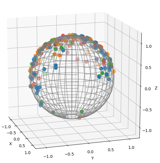
(a)

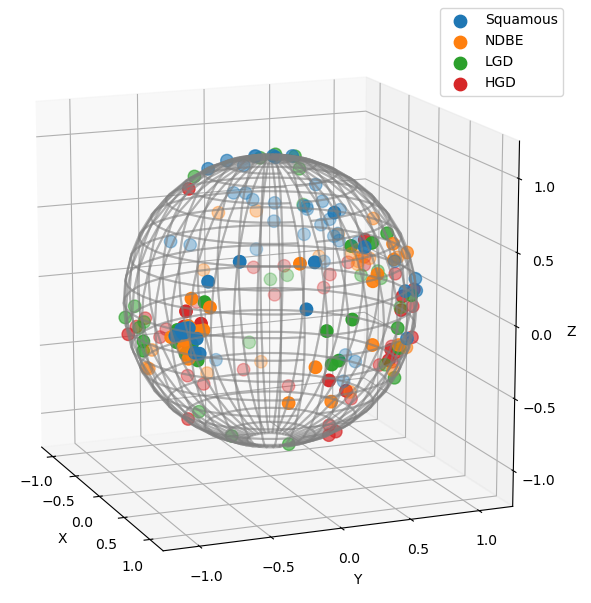
(b)

Figure 3.3: Visualization of Latent Space for model $\mathcal{S}$-AE with $M=3$ without and with spread loss. The same batch of 200 images was encoded by both models, and different image classes are visualized with different colored points. Although not entirely evenly spaced, the points encoded by the model trained with spread loss cover a significantly larger area of the sphere.

In this figure, we can see that implementing spread loss has a clear effect on the distribution of encoded images over the latent space. While in the regular $\mathcal{S}$-AE , the points are mainly concentrated on one side and the upper half of the sphere, with spread loss, those points are more evenly distributed over the sphere surface, leaving less significant gaps in the informedness of the latent space. We therefore predict that with this loss, a structured and uniformly informed latent space is obtained, which will allow us to use the proposed $\mathcal{S}$-AE as a generative model, while still retaining the benefits of autoencoders, such as stability and sharpness of reconstructions.

3.5. Roto-Equivariant Variational Autoencoder

Besides comparing the different geometric latent spaces, we also experiment with learning representations that are orientation-disentangled. CNNs are, by design, equivariant to translation. This means that translating the input will also transform the learned representation accordingly. The same does however not hold for orientation information, causing identical patches in different orientations to result in different learned representation vectors. As biopsies can be scanned in any arbitrary orientation, this redundant information thus becomes entangled in the learned latent space, possibly making the representations harder for the model to process. It would therefore be beneficial to remove this rotation information and create roto-disentangled representations.

Lafarge et al. propose that learning such representations relies on two factors: extending the encoder and decoder networks to be group-structured, which makes the network equivariant to rotations, and then leveraging this structure to separate oriented and non-oriented features in the latent space, which results in disentangled representations. The following section will describe how this is accomplished, providing some necessary mathematical preliminaries of group theory, explaining the concepts of group-convolutional neural networks, and describing how these concepts can be used to achieve roto-disentangled representations.

3.5.1.  Group Convolutional Neural Networks

Group Theory

A group $G$ is a set of elements performing a group operation, that together satisfy properties of closure, associativity, presence of the identity element, and that each have an inverse Herstein (1991). When such a group operates on a set, this is called the group action. Formally, a group action of $G$ on a domain $X$ is defined as a mapping in which every group element is associated with some element in $X$, such that the mapping from $G$ to the permutation group of $X$ is a homomorphism. Such a domain is known as the G-space. Each group element can be represented as a matrix that acts on, or transforms, an element of the G-space, a mapping also known as the group representation $\rho$. Multiple types of group representations exist. For this work, most important are the trivial representation, which maps any vector to itself, and the regular representation, which maps all the axes in a representation space to another basis Weiler and Cesa (2019).

Regular Group-Convolutional Neural Networks

In theory, regular convolutions can be generalized to such a group framework by viewing the convolutional kernel as the G-space on which elements of the group of translations ($\mathrm{T}$) act. Considering a neural network’s convolutional layers in this way, allows us to more easily see how group convolutions can extend the model to be equivariant to rotations as well. Instead of the group $\mathrm{T}$, we simply extend to the finite subgroup $SE(2,N)$ of the continuous translation-rotation group $SE(2)$, where $N$ is the cyclic permutation order. Hence, we can achieve roto-translational equivariance by extending the VAE model encoder and decoder networks from regular convolutional neural networks to Group-Convolutional Neural Networks (G-CNNs) Cohen and Welling (2016a).

G-CNNs generally consist of three main elements that set them apart from a regular CNN: a lifting convolution, the group convolutions, and a projection operation. The lifting convolution discretizes the orientation axis of an image by transforming the image features for every rotation angle $\frac{2\pi}{N}n$, with $n\in\{0,\dots,N-1\}$. The internal feature maps can be treated as SE($2$) images $F\in\mathbb{L}_{2}[SE(2,N)]$. Next, these are convolved with image kernels in the group convolution layers of the network, preserving the channels and ensuring equivariance under the action of the $SE(2,N)$ group. Hence, in both group lifting and convolutional layers, information about orientation and translation is preserved. Our goal however, is to obtain an invariant representation, which requires a final projection layer. This layer performs a projection with an operation that is invariant to the group action, such as summing, maxing, or averaging, resulting in a representation from which orientation and translation-information is lost.

Steerable Group CNNs

One possible downside of the above framework is that the values of the group convolutional feature maps are computed and stored on each element of the group. The computational complexity of the model thus scales with the order of the group that is used. Cohen and Welling (2016b) therefore propose a more general framework through steerable G-CNNs. Steerable G-CNNs apply do not learn a signal directly, as is the case for G-CNNs, but instead learn to describe it through functions decomposed by a Fourier transform. In our case this is a transform of signals over the orthogonal $SO(2)$ group, which a subgroup of $SE(2)$ that concerns only continuous rotations and no translations. By applying the Fourier transform, steerable group convolutions are expanded to the co-domain, instead of to an additional axis in the domain as is the case for regular group convolutions. The functions, or feature vectors, in the resulting feature fields can be interpreted as Fourier coefficients. The transformation laws of these fields are determined by the group representation type that is associated with it. This not only allows for more efficient memory storage, but presents a more precise way of describing signals than in regular G-CNNs.

3.5.2.  Learning Roto-Disentangled Representations

Having obtained encoder and decoder networks that are roto-translational equivariant, we can partition the latent space to encode both isotropic and oriented image features, thereby creating disentangled representations. Following Vadgama et al. (2022), we choose to work with the more efficient steerable G-CNN type network as explained above. These networks, like regular G-CNNs, contains three key layers: a lifting layer, which requires the trivial representation type as input in order to lift the input image’s feature space, a series of regular representation type steerable convolution layers, and a projection layer.

We then have our steerable encoder model learn three different quantities: a latent mean descriptor $\mu$ that is equivariant under the actions of the group $SE(2,N)$, a pose or orientation corresponding to this representation $\mathbf{R}$, and an invariant scalar parameter that either corresponds to $\kappa$ in the case of the hyperspherical framework, or $\sigma$ in the case of the regular Gaussian posterior. Because the architecture is equivariant, rotating the network’s input results in a transformation of both the mean descriptor $\mu$, as well as the estimated pose $\mathbf{R}$ via a representation of the group, whereas the predicted parameter $\kappa$ or $\sigma$ stays invariant. The network’s equivariance allows us to essentially undo the rotation of the mean descriptor and orient it to a canonical pose via the mapping $\mu_{0}=\rho(\mathbf{R}^{-1})\mu$, with $\rho(R)$ a group-representation of SO(2). Thus, our method obtains an invariant descriptor $\mu_{0}$ that represents a whole equivalence class of images that are just rotated copies of one another. The main learning objective is thus to learn a probability distribution on this equivalence class, which is done as usual through variational inference. For the decoding process, we sample a vector $\hat{z}_{0}$ from this distribution, map it to its corresponding learned pose $\mathbf{R}$, and feed it through the equivariant decoder network. This results in a reconstructed image that has the same orientation as the original input image.

Section 4. Experimental Set-up

Our goal is to evaluate whether the geometrically-inspired VAEs introduced in Section 3, can be used to model the progression of BE in a more meaningful way than regular VAEs. We therefore test all models on a variety of tasks, meant to evaluate the quality of the learned representations in both a quantitative and qualitative way. We conduct experiments with reconstruction loss, classifiability of latent vectors, random generative sampling quality, and the ability to generate smooth interpolations. This section will detail the exact setup for conducting these experiments. Section 4.1 will start by giving an overview of what datasets were used, how these were obtained, and how the data was processed. Next, Section 4.2 will give a detailed overview of the model architectures, hyperparameter choice and training procedure. Finally, Section 4.3 will describe how we will evaluate the quality of the learned representations and motivate the choice for these experiments.

4.1. Data

To test whether the proposed methods can learn to model the progression of BE in an unsupervised setting, we train them on histopathological image data containing instances of the four different progression stages. The sources and format of this data are discussed in Subsection 4.1.1, and the processing of the data is discussed in Subsection 4.1.2.

4.1.1.  Datasets

We train our models on digitized H&E-stained endoscopic biopsies. Four separate datasets containing such scans are obtained. The ASL and RBE datasets consist of annotated biopsies from archived BE screenings from the Amsterdam University Medical Centre (AMC). Furthermore, the LANS dataset consists of cases from the Dutch expert board of esophageal cancer (Landelijk Adviesorgaan Neoplasie Slokdarm). As mentioned before, the interobserver variability between pathologists can be very high, which could make the annotations made by the individual pathologists of the ASL, RBE and LANS datasets less reliable. A study by van der Wel et al. (2020) therefore set out to study this variability and create a dataset with more reliable annotations. This dataset, BOLERO (Barrett mOlecuLar ExpeRt cOnsensus), contains biopsies that were each assessed by a review panel of 4 expert BE pathologists, with a total test panel of 51 pathologists from over twenty countries. The study found that pathologists overall had a good concordance for distinguishing non-dysplastic and dysplastic BE, with agreeability rates for NDBE and HGD being almost 80%, but that the distinction between LGD and HGD was harder to make, leading to a rate of 40 % for LGD.

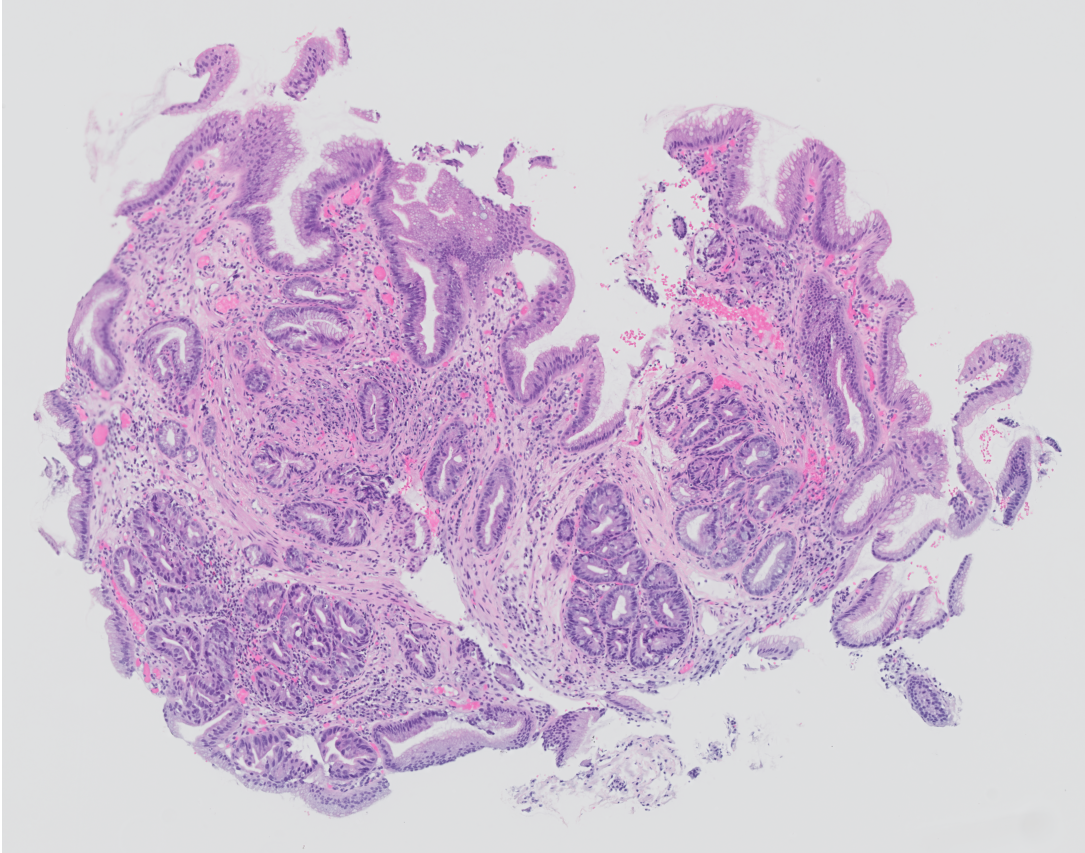
Figure 4.1: Example of a scanned endoscopic biopsy.

Combining these four datasets leads to a total number of 934 biopsies from 324 patients. All biopsies are stored in a format known as a Whole-Slide Image (WSI). Whole-slide imaging is also known as virtual microscopy and stores highly precise scans of a glass slides, containing up to four biopsies from the same patient, at multiple microscopic magnification levels ranging from $5\times$ to $40\times$ Li et al. (2022). An example of one such biopsy at the lowest magnification level is shown in Figure 4.1. Pathologists examine these images with specialized software and divide the entire biopsy into designated regions of a specific type of cell tissue. For the current dataset, these are background, where no cell tissue is present, stroma, which is connective tissue between cells, and the four classes used for diagnosing BE: squamous epithelium Non-Dysplastic Barrett’s Esophagus (NDBE), Low-Grade Dysplastic Barrett’s esophagus (LGD) and High-Grade Dysplastic Barrett’s esophagus (HGD). For these last four categories, the annotations are made at glandular level by manually tracing around tissue regions. Except for the BOLERO dataset, which was annotated by panels of multiple pathologists, all annotations are made by a single expert-level histopathologist and are in accordance with case-level diagnoses of biopsies made by a review panel.

4.1.2.  Preprocessing the dataset

As can be observed in Figure 4.1, a biopsy contains multiple types of tissue and many fine-grained details. Whole-slide images composed of up to five biopsies therefore contain an enormous amount of data. Files of this format are often larger than 1 GB and typically contain more than $100.000\times 100.000$ pixels. Hence, it is essential to preprocess the data to allow deep learning models to perform computations with it. Most studies working with WSI files choose to divide the image into smaller standard image format patches. Multiple approaches to determining these patches exist, however, by far the most common method is to simply divide the WSI uniformly into smaller patches of the same size Li et al. (2022).

Determining Patch Area

Following the uniform slicing approach, a number of important choices remain to be made in regard to what information is contained within the patches. One such choice is the patch size, which is closely interlaced with the microscopic magnification level. Ideally, we want to create patches that, when individually processed by the model, contain enough information for the model to be able to recognize certain stages of BE. This means that a somewhat larger area of the WSI should be covered in each patch, such that general changes in cell morphology can be observed. However, we are limited in the image resolution of the patches we create, as VAEs generally work with somewhat smaller image sizes (Thambawita et al., 2021). Additionally, we found that hyperspherical model types tend to be less numerically stable than normal-type VAEs, and that larger patches increase the already heavier computational power required for roto-equivariant model types. Since we want to equally compare performance across all different models, we choose to have a resolution of $64\times 64$ for each image patch, allowing all models to easily process them. Within this patch size, we then want to contain as much information about the cell tissue as possible. We show $64\times 64$ patches of $5\times$ and $10\times$, the lowest possible magnification levels, to an expert-pathologist and biomedical scientist, who both indicate that $10\times$ patches, unlike $5\times$, do not contain enough context to accurately make a classification. To illustrate this, four examples of patches with different magnification levels are shown in Figure 4.2. For $5\times$ magnification, some patches still do not cover enough of the biopsy to make a perfect classification, but for many patches, clear cases of squamous NDBE, LGD and HGD type tissue can be observed. We therefore choose to work with the $5\times$ magnification patches.

(a) $5\times$

(b) $10\times$

(c) $5\times$

(d) $10\times$

Figure 4.2: Comparison between different magnification levels. All patches are of size 64$\times$64 and were taken from the same biopsy.

Discarding Low-Context Patches

To further increase the amount of context present in the patches, we choose to only include patches in our final dataset that contain a high enough threshold of relevant tissue. By relevant tissue, we mean belonging to either the squamous, NDBE, LGD or HGD classes, meaning that background and stroma are excluded. This design choice was determined in accordance with a histopathologist, who argued that pathologists disregard the background and stroma classes when determining BE. As such, only patches containing 50% or more data annotated as belonging to the relevant classes are selected. This threshold was determined heuristically by experimenting with several threshold values. A number much higher than 0.5 was found to lead to a too significant reduction in the total amount of patches included in the final dataset, while a lower threshold resulted in a large number of low-context patches that were difficult for a histopathologist to classify. With a threshold of 0.5, an image resolution of $64\times 64$ and a magnification level of $5\times$, we create a dataset containing a total of 75.661 patches.

Computing Labels and Balancing the Dataset

Although this work studies unsupervised representation learning, we nevertheless want to obtain labels for the individual patches as well. The reason for this is twofold. First, biopsies are known to contain a large amount of squamous and NDBE-type tissue, and less LGD and HGD. Because we want the model to be trained on all different instances of the progression stage equally, there is a need to balance the training dataset. We therefore require patches to be labeled in order to know which ones to include in the training set. Second, as will be discussed more in-depth in Section 4.3, we conduct experiments into the classifiability of the learned representation vectors. To evaluate the experiments, we compute classification accuracy, a metric which requires ground truth labels. Hence, labels are computed for every individual patch.

These labels are computed according to annotations made by the pathologist, which are contained in a mask file accompanying each WSI. The format of these mask files is such that all pixels within a traced region designated by the pathologist to belong to a certain class, are assigned an integer value corresponding to that class, i.e., $0$ for background, $1$ for stroma, $2$ for squamous, and so on. This results in an image file consisting of only six possible pixel values, that encode the pathologist’s annotations in a way that can easily be processed. In all four different datasets, such a mask file is provided for the WSIs. When dividing the WSIs into smaller patches, we therefore also divide the corresponding mask files into the same format.

We then convert these masks into scalar labels, so that they can be used to evaluate our models’ performance. To do so, we choose to take the most dominant class, or in other words the most commonly occurring pixel value within a patch, as its label class. In doing so, we discover a class imbalance in our dataset: 16.1% of the patches are labeled as squamous, only 11.9% as HGD and 11.5% as LGD, while a great majority of 60.5% are labeled as NDBE. Because we want our model to be exposed to instances of classes equally during training, we decide to stratify the dataset. For each class, we take the 8000 patches with the highest dominance of the corresponding class pixel, leading to a balanced dataset with 32.000 patches that contain the most clear cases obtainable within each class.

For our model pipeline, we choose to use the patches belonging to the ASL, RBE and LANS datasets as training data and those belonging to BOLERO as test data. In this way, we expose the model to a variety of unlabeled training data and evaluate it on an unseen dataset with far more reliable labels as compared to the other datasets. We can therefore fairly asses both the generalization capabilities of our models, and determine how well they pick up on the different classes during training. We also designate 10% of our training set as validation dataset.

4.2. Models and Training

In Section 3, we explained a number of different concepts that could improve the structuring of the VAE’s learned latent space. These were the Riemannian latent space of RHVAE, and the hyperspherical latent space of $\mathcal{S}$-VAE . Moreover, we described how the hyperspherical VAE could be extended to be roto-equivariant, as proposed by Vadgama et al. (2022). Finally, we proposed a modification of the hyperspherical setup to a non-variational autoencoder framework.

To test which model provides the best latent structuring, we compare RHVAE and $\mathcal{S}$-VAE to a baseline vanilla VAE, which we will refer to as $\mathcal{N}$-VAE , where $\mathcal{N}$ stands for the Gaussian distribution. Secondly, to assess the possible benefits of the roto-equivariant $\mathcal{S}$-VAE , we build and compare such equivariant versions of $\mathcal{S}$-VAE and $\mathcal{N}$-VAE , as detailed in Subsection 3.5. Finally, to test the validity of our own proposed spherical autoencoder framework ($\mathcal{S}$-AE ), we create non-variational autoencoder variants of both equivariant and non-equivariant hyperspherical and normal-type models. Unfortunately, experiments for RHVAE could not be conducted, as the mode failed to generalize to large datasets. This will be further elaborated on in Subsection 4.4. The remaining sections will focus on the other models described above, and we will conduct experiments for a total of eight different models: $\mathcal{N}$-VAE , $\mathcal{N}$-AE , equivariant $\mathcal{N}$-VAE , equivariant $\mathcal{N}$-AE , $\mathcal{S}$-VAE , $\mathcal{S}$-AE , equivariant $\mathcal{S}$-VAE and equivariant $\mathcal{S}$-AE .

4.2.1.  Model Architectures

In order to compare the different models fairly, we follow an almost identical architecture for all models. As Lafarge et al. demonstrate good results on histopathological data with their vanilla and roto-equivariant VAEs, we base our architecture on theirs. A detailed schematic overview of the architecture can be found in Appendix A. In general, the base encoder architecture consists of three ConNeXt blocks Liu et al. (2022), containing a convolution layer with kernel size 5, followed by a layer normalization, a pointwise convolution, a GELU activation, and another pointwise convolution. Each block is followed by a max pooling operation with kernel size 2. The decoder mirrors this structure, swapping out the convolutional blocks for their transposed versions and replacing the pooling operations with upsampling operations. We furthermore pad our input images to be of size 68 $\times$ 68, to ensure that all convolutions can be computed.

In case of the non-equivariant variational versions of $\mathcal{N}$-VAE and $\mathcal{S}$-VAE , the encoder outputs the parameters for the relevant posterior distribution: a vector $\mu$ and an isotropic scalar $\sigma$ or $\kappa$. Additionally, for spherical models, the softmax operation is applied over $kappa$ and a value of 1 is added, ensuring a minimum variance of 1. Besides the distribution parameters, a third parameter coding for the orientation of the input $\mathbf{R}$ is also learned in the equivariant setting. Moreover, in the equivariant framework, all convolutional layers are replaced by their group variants and the remaining layers are adapted for use with the extended channel format. We choose to follow Vadgama et al. and use the $C_{8}$ cyclic permutation group for all group convolutions, leading to a model that is equivariant to eight rotations covering $SO$(2), or rotations of angles of 45 degrees.

For the normal non-variational autoencoder type models, $\mathcal{N}$-AE and equivariant $\mathcal{N}$-AE , we do not learn the log variance parameter $\sigma$ and instead take the learned vector $\mu$ directly as our latent encoding $\mathbf{z}$. In the case of the spherical autoencoder model types $\mathcal{S}$-AE and equivariant $\mathcal{S}$-AE , as described in 3.4, we do not omit the concentration parameter $kappa$ completely, but instead fix it to a value of 1000, which was heuristically determined to fully limit the vMF distribution’s variability.

4.2.2.  Model Hyperparameters

As the dimensionality of the latent space can have great influence on the models’ output, we test a range of different latent dimension sizes. Lafarge et al. use a dimensionality of $M=64$, so we choose to vary around this number, leading to a total of eight different sizes $M\in(3,8,16,32,64,128,256,512)$. It is worth noting that we choose a multiple of 8 because of the $C_{8}$ group, which also limits the latent dimension of equivariant type models to have a minimum size of 8. Although we cannot use a latent dimension size lower than 8 for equivariant models, we nonetheless chose to include 3 in our range of sizes because of its property of being visualizable. This allows us to visually inspect the latent space and verify that the proposed methods are indeed following a different geometric structuring of the manifold.

Avoiding Numerical Instability

Another important factor in choosing the latent space sizes, is that spherical variational model types can become numerically unstable in higher dimensions Davidson et al. (2018). We found that for latent dimensions of 32 and higher, the model started outputting NaN (Not a Number) values, and the spherical variational models could not be trained. Davidson et al. propose this can in part be explained by the vanishing surface problem. Considering the equation for the surface of a hypersphere

$$\mathcal{S}(m-1)=r^{m}\frac{2(\pi^{m/2})}{\Gamma(m/2)},$$ (4.1)

it can be observed that in the infinite limit of dimension $m$, the surface area of the hypersphere approaches 0. The authors moreover already observe this vanishing surface problem in dimensions sizes higher than 20. This observation corresponds to our preliminary experiments, as a dimension of 16 could still be trained, while 32 unfortunately failed. We observed that the same does not hold for spherical autoencoder models, however, suggesting that the concentration parameter $\kappa$ plays an important role in the numerical instability. We therefore implement a way to limit the minimum value for $\kappa$, which normally can range between 1 and 10000. Using $\kappa=100$ as our minimum value, we are able to train equivariant and non-equivariant spherical VAEs up to a dimension size of 256, albeit at the cost of somewhat limiting the expressivity of the model. The latter will be taken into account when analyzing the results.

4.2.3.  Training Details

We then train all our models for 500 epochs, with a batch size of 128. We employ the Adam optimizer with a learning rate of 0.0005 and use a cosine annealing learning rate scheduler. Preliminary experiments reveal that all models can reach convergence with these settings. Prior to training, input images are padded to size 68 $\times$ 68 and normalized. Moreover, as mentioned in the previous section, we use MSE loss for all models as reconstruction loss. Since our equivariant models, due to rotations during training, lose out on information about the outer edges of an image, we choose to disregard these areas when computing the reconstruction loss. Furthermore, we determine regularization loss by computing KL divergence for variational model types and add this to the reconstruction loss.

4.3. Evaluation of Proposed Methods

In this study, we seek to learn how providing different forms of geometric structure to a VAE’s latent space can make representations of histopathological data more meaningful. This leads to the question of what is actually meant by a meaningful representation. In this section, we therefore aim to provide the reader with an overview of the conducted experiments and motivate why they inform us about the quality of the learned representations. For quantitative evaluation, these experiments include reconstruction error and classifiability of latent representations. Furthermore, for qualitative evaluation, we experiment with random generative sampling and interpolation quality.

Reconstruction Error

In all autoencoder frameworks, an image is compressed into a lower-dimensional representation by the encoder network and consequently reconstructed from this representation by the decoder. It naturally follows then, that the quality of the representation has a direct influence on the reconstruction. The more relevant features a model learns to encode in the latent space, and conversely the more irrelevant data it learns to discard in its encoding, the better the decoder will be able to create a reconstruction. We therefore quantitatively evaluate performance by reporting the reconstruction loss, which for all models is calculated using the MSE loss. During the reconstruction experiments, we subtract the outer edges of each image from the loss for both equivariant and non-equivariant models, so that the area to be reconstructed is equal across all model types, and the losses can be compared fairly. After training, we apply each model to the unseen Bolero test set. A lower loss value means a reconstruction closer to the input image and indicates a more meaningful and informative latent representation.

Classification of Latent Representations

In the field of supervised learning of histopathology data, a CNN classification network receives image patches and learns to directly map them to their correct classes. Many different approaches to this problem have been proposed, but general performance is good, with many proposed methods reaching 80-90% accuracy scores de Souza Jr et al. (2018). It would therefore be interesting to replace the input of this type of classifier model with the latent representations learned by our VAEs. In this way, we can directly measure how accuracy scores are affected by differently-structured latent representations. If, for example, spherical type models improve the structuring of the latent space in a meaningful way, for instance by an improved clustering ability over the vanilla VAE, then this would naturally lead to a higher ease of classification and a better classification accuracy.

We therefore train models for classifying both representation vectors and original image patches. For our latent representation classifier, we use a simple MLP with three linear layers. Latent vectors encoded by a pre-trained model are forwarded through the model with a hidden dimension of 64 and mapped to a vector containing four outputs, of which the values code for the four class probabilities. We train this model for 500 epochs, use Cross Entropy to compute loss, and report accuracy scores for all models and latent dimension sizes. Furthermore, to compare the accuracy scores of the representations to those of patches, we create a convolutional neural network that follows the same architecture as the VAE encoders described earlier. Both a regular convolutional network and an equivariant group-convolutional network are tested. We take the encoder network architectures of both variants and add an MLP head identical to the one used for the representation classification. The models are then trained in an identical setting to the representation classifiers, allowing for a fair comparison of classification ability between representations and image patches.

Random Generative Sampling

Besides the quantitative evaluation methods, we moreover evaluate the method in a qualitative way. One way to achieve this is to randomly sample new images from each of the models’ latent spaces and visually determine their quality. We generate new images by sampling from the prior for all models except the autoencoder types, for which we simply decode a vector from a uniformly random location on the latent space. Sampling from a number of locations on the latent space can provide insights into how such a manifold space is structured. If, for example, there are many low-density areas in the space, then that will be reflected in the quality of samples originating from such an area. Conversely, if many random samples are high quality, this would suggest that the latent space is well-structured.

Besides general qualitative analysis, the generative sampling experiments will also be used to assess the ability of $\mathcal{S}$-AE and equivariant $\mathcal{S}$-AE models to be used as a generative model. Ordinary AEs will for most samples result in nonsensical images, and because of this are not considered a generative model. Examining images generated by $\mathcal{S}$-AE can thereby demonstrate to which capacity it can be used as a generative model.

Interpolations

Finally, we examine the models’ ability to create smooth, realistic interpolations. Similarly to generative sampling, when interpolating, we sample and decode vectors from the latent space. However, unlike above, we do not sample from a random location on the latent space, but sample along the shortest path between two images in the latent space. For normal-type models, this means a linear path, while for Riemannian and spherical-type models, we sample along the geodesic. In both Chadebec et al. (2020) and Davidson et al. (2018), interpolations were used to demonstrate the improved latent structuring of the geometric VAE models. Interpolations appeared smooth and were able to retain more realistic structure of objects. Ideally, we would want to be able to observe similar realistic variations in the morphological structure of cells for the current work. Such an interpolation would be an indication of a well-structured latent space, that is able to capture elements about the progression of healthy tissue to Barrett’s esophagus.

4.4. Motivation for Not Continuing with RHVAE

Unfortunately, we found that it was impossible to train RHVAE with our full dataset. As described in Section 3.2, the Riemannian metric is computed by a neural network, and this network is parameterized by the data points. The model complexity therefore scales with the size of the dataset, which in our case includes 32.000 data points. Such a size lead to infeasible computation times.

When conducting initial experiments with RHVAE, the default settings as provided by the authors were used. This means that the encoder and decoder networks, and the network for learning the Riemannian metric, all consist of two linear layers, separated by a ReLU activation. The hyperparameters required for computing the metric in RHVAE are also kept at default, leading to a temperature of $T=1.5$, and a regularization parameter of $\lambda=0.01$. Multiple dataset sizes were tried out, but we found that a dataset of 1000 points already increased training time by such an amount that it became infeasible to compute. Attempts were made to reduce this by increasing the amount of data points included in one centroid, leading to a lower number of centroids in total. This somewhat increased the number of training points that were able to be used for training, however, it still could not come close to the magnitude of the 30.000 patches that are available. Experiments were also done with different neural network architectures, both for the Riemannian network as well as the encoder and decoder networks, and multiple different latent dimension sizes were tested. However, decreasing the complexity of these models did not have an effect on the infeasibility of the computation time.

To gain insight into the general performance of RHVAE for pathological images, we then experimented with smaller dataset sizes and trained the model with datasets of 100 and 400 data points. Examples of reconstructions made by these models are shown in Figure 4.3. In both dataset sizes, we see that reconstructions are often not true to the original. Although it would be expected that reconstructions of an insufficiently trained model would appear as a less sharp version of their originals, here instead we see instances of reconstructions containing a completely different tissue pattern than their original input.

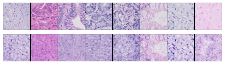
(a) Dataset size = 100

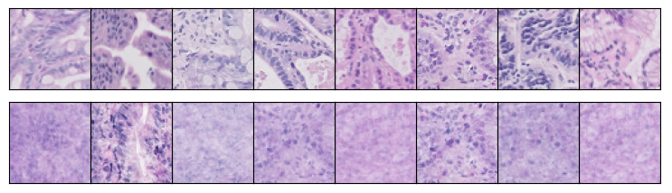
(b) Dataset size = 400

Figure 4.3: Reconstructions made by RHVAE for different dataset sizes. The top row shows the original patches and the bottom row the reconstructions.

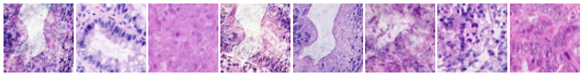
(a) Dataset size = 100

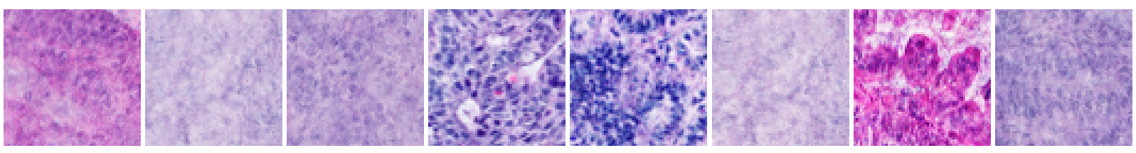
(b) Dataset size = 400

Figure 4.4: Randomly generated images from the latent space learned by RHVAE for models trained with different dataset sizes.

It can also be observed that some structures appear multiple times, which becomes especially apparent in Subfigure 4.3(b). These results suggest that the model might be overfitting and is inappropriately applying the patterns that it has learned to the reconstructed patches. Another indication of overfitting becomes apparent from Figure 4.4, which shows some examples of randomly generated images. For the model trained with 100 data points especially, the images look somewhat realistic, but the same structures are being repeated over different generated images. For a dataset size of 400, this problem becomes less apparent, but the generated image quality suffers.

Finally, Figure 4.5 shows a visualization of a 3-dimensional latent space learned by RHVAE. Subfigure 4.4(a) shows the four different classes visualized as differently colored points. It can be seen that some clustering exists, with clusters for squamous and high-grade dysplasia becoming the most apparent out of the four progression stages. This is in line with the nature of the data, as these two classes are also known for being the least difficult to differentiate in histopathology as well van der Wel et al. (2020). Furthermore Subfigure 4.4(b) shows the same latent space, but points are colored in accordance with the value of the log determinant of the metric tensor $\sqrt{\det(\mathbf{G}(z)}$, which corresponds to the volume element of the learned manifold.

(a) Training images belonging to different classes visualized in the latent space.

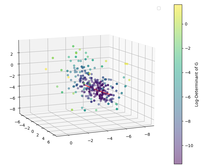
(b) The geodesic follows the most informed path, visualized here by $\sqrt{\det(\mathbf{G}(z)}$.

Figure 4.5: Two visualizations of training points embedded in the latent space learned by RHVAE with M=3.

A lower value indicates a higher density of data points and therefore a more informed region within the manifold space. A geodesic between two random data points is calculated through the Riemannian metric and also plotted in red. It can be seen that this path does not appear as a straight line, which would be the case for a Euclidean distance, but rather as a curve. Moreover, this curve follows the direction of the highest density, creating a path that passes through the most informed region of the manifold space.

Although the clustering ability to some extent indicates the suitability of RHVAE for the current pathological use case, the earlier reconstructions and generations indicate that the model has a tendency to overfit for very small dataset sizes, and fails to generalize well for slightly larger datasets. This, combined with the severe limitation of dataset size, lead us to decide to not run further experiments on RHVAE and instead focus efforts on the remaining models.

Section 5. Results

This section will discuss the results of the experiments as described in Section 4.3 on the spherical VAE, and its roto-equivariant and autoencoder variants. First, in Section 5.1, reconstruction quality will be assessed. Secondly, in Subsection 5.2 the results for classification tasks will be discussed. Next, Section 5.3 will provide the results of the generative experiments, first examining the quality of random generative sampling, then providing some examples of interpolations. Finally, Section 5.4.1 will examine the potential of spherical autoencoders as a generative model, by showing generative samples, interpolations, reconstruction errors, and classification accuracies for models with spread loss implemented.

5.1. Reconstructions

Using the training settings as discussed in the previous Section 4.2, we evaluate the models’ ability to retain important features in their learned representations by reporting final reconstruction losses on the unseen Bolero test dataset for all models and latent dimensions sizes. For performance on training and validation set, see Appendix B.1. Although spherical VAEs could not be trained for a latent size of 512, as discussed in Subsection 4.2.2, we still include results for this dimension size for other model types. The results on the test set are shown in Table 5.1.

Table 5.1: Reconstruction Losses on Test Dataset

	Normal				Spherical
	Non-Equivariant		Equivariant		Non-Equivariant		Equivariant
$M$	$\mathcal{N}$-VAE	$\mathcal{N}$-AE	Eq. $\mathcal{N}$-VAE	Eq. $\mathcal{N}$-AE	$\mathcal{S}$-VAE	$\mathcal{S}$-AE	Eq. $\mathcal{S}$-VAE	Eq. $\mathcal{S}$-AE
$3$	1895.56	2013.46	-	-	1930.60	2089.98	-	-
$8$	1807.06	1769.14	2103.47	2103.35	1707.14	1743.25	2103.66	2103.27
$16$	1635.89	1621.97	1290.60	1252.64	1563.19	1607.79	1303.07	1313.58
$32$	1435.60	1428.11	1161.32	1134.30	1389.64	1403.93	1142.24	1135.50
$64$	1260.85	1273.44	993.94	988.42	1250.45	1258.50	1009.90	992.39
$128$	1092.88	1113.56	857.40	853.79	1133.33	1104.18	902.82	853.75
$256$	904.53	935.09	710.22	706.50	1056.68	925.07	826.10	703.88
$512$	748.42	736.92	562.11	556.61	-	727.06	-	540.13

From this data, we can observe multiple things. First of all, the higher the latent dimension size, the lower the reconstruction loss and the better quality the reconstruction is. Since a higher latent dimension allows for less compression of features, this is to be expected. To provide some context to these loss values, we show examples of reconstructed images for dimensions 8, 64, and 256 for the $\mathcal{S}$-VAE model in Figure 5.1(a). Here we can indeed observe the same trend of higher dimensions leading to better reconstructions. However, we can also see that even the highest dimension size that is currently possible to use for the $\mathcal{S}$-VAE model, 256, still does not recover the original image completely. The same is true for the model with the lowest reconstruction error, the equivariant spherical autoencoder, as is shown in Figure 5.1(b). More details are recovered compared to for instance a latent size of 8, which only retains general shapes, but the reconstructions are still blurry compared to the originals. This suggests that the finer details are difficult to compress and that this fact should be taken into account when interpreting further experiments.

When comparing different model types, we first look at normal vs spherical types. In general, it becomes apparent that spherical models have an edge over normal-type models in the lower to medium dimensionality range. For instance, $\mathcal{N}$-VAE and $\mathcal{N}$-AE perform better than their spherical counterparts with a latent size of 3, but $\mathcal{S}$-VAE and $\mathcal{S}$-AE perform better by a rather large margin in dimensions 8-32. From dimension sizes of 64 onward, this advantage becomes smaller, and from 128 to 512, normal-type models achieve lower reconstruction losses compared to spherical models.

Furthermore, comparing non-equivariant models to roto-equivariant models, it can be observed that equivariant models perform much better than non-equivariant ones in all dimensionalities except 3, where there is no data available, and 8. Finally, comparing variational autoencoders to their non-variational variants, we see that autoencoders consistently obtain lower reconstruction errors. This effect becomes more apparent in higher dimensions. Moreover, the difference between variational and non-variational is especially noticeable between spherical models.

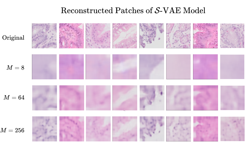
(a) Reconstructions of $\mathcal{S}$-VAE model for latent dimension sizes of 8, 64 and 256.

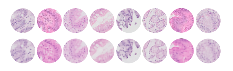
(b) Reconstructions of equivariant $\mathcal{S}$-AE with $M=512$, the model with the lowest reconstruction error.

Figure 5.1: Examples of reconstructed image patches.

5.2. Classifications

Having learned latent representations, we analyze their expressivity by reporting the test accuracy of a linear classifier network. The results of these experiments are shown in Table 5.2. First of all, in terms of latent dimension sizes, we see a different trend than for the reconstruction losses. Unlike in the reconstruction loss experiments, a higher latent dimension size does not lead to improved results. Although the lowest dimension sizes of 3 and 8 still lead to the poorest results overall, here dimensions 32 and 64 achieve the highest accuracy consistently over all models, with the overall best score being achieved by the equivariant spherical VAE of dimension size 32. Higher sizes such as 128 to 512 achieve comparable results on non-equivariant normal type models, but are considerably lower in case of the equivariant spherical autoencoder. For spherical models with a dimension size of 256 for example, non-equivariant versions achieve scores around 0.4, while the equivariant autoencoder only achieves 0.24, indicating a random guess in case of our four possible classes.

In terms of equivariance, it can be observed that for a latent dimension of size 32, equivariance improves the performance of both normal and spherical models. For spherical models in particular, equivariance has a slight positive effect on the accuracy scores in dimensions higher than 8. For normal-type models, equivariance does not differ much from non-equivariant accuracy scores in these dimension sizes. Furthermore, we can also observe that in general, autoencoder-type models achieve comparable or slightly worse scores than their variational counterparts, suggesting that representations learned by variational models are slightly easier to classify. All in all, these trends differ from the ones observed in Table 5.1, suggesting that a representation having a lower reconstruction error does not necessarily correlate with it being easier to be classified.

Table 5.2: Classification Accuracy of Latent Representations on Test Dataset

	Normal				Spherical
	Non-Equivariant		Equivariant		Non-Equivariant		Equivariant
$M$	$\mathcal{N}$-VAE	$\mathcal{N}$-AE	Eq. $\mathcal{N}$-VAE	Eq. $\mathcal{N}$-AE	$\mathcal{S}$-VAE	$\mathcal{S}$-AE	Eq. $\mathcal{S}$-VAE	Eq. $\mathcal{S}$-AE
$3$	0.248	0.255	-	-	0.250	0.262	-	-
$8$	0.333	0.348	0.342	0.171	0.363	0.325	0.228	0.274
$16$	0.387	0.395	0.394	0.420	0.400	0.343	0.351	0.298
$32$	0.408	0.396	0.466	0.462	0.414	0.308	0.478	0.455
$64$	0.454	0.395	0.398	0.414	0.391	0.409	0.417	0.433
$128$	0.422	0.424	0.398	0.397	0.396	0.393	0.412	0.282
$256$	0.422	0.423	0.380	0.398	0.400	0.406	0.408	0.243
$512$	0.382	0.363	0.380	0.389	-	0.371	-	0.254

To provide context for these accuracy scores, we also report accuracy scores on an image patch classification task using a CNN. These accuracy scores are shown in Table 5.3. In general, accuracy scores for the CNN lie around 0.45 to 0.55. Compared to the latent representations, they are more consistent over different dimension sizes, with the 256 having the best score overall for the non-equivariant CNN and the equivariant CNN reaching the highest score of 0.543 with a latent dimension of 64. The trend of the representations performing best in the mid-range of dimension sizes does not hold for the CNNs, although it is the case that equivariance improves results for both experiments. In general however, the CNN’s results are only slightly higher than the best accuracy scores for the classification of latent representations, suggesting that these models learn representations that have not lost too much relevant information compared to the original images.

Table 5.3: Classification Accuracies of Image Patches on Test Dataset

$M$	Non-Equivariant	Equivariant
$3$	0.455	-
$8$	0.478	0.452
$16$	0.474	0.518
$32$	0.460	0.495
$64$	0.450	0.543
$128$	0.469	0.512
$256$	0.505	0.496
$512$	0.465	0.514

5.3. Generative Quality

5.3.1.  Generative Random Sampling

To gain sights into the structure and general informedness of the learned latent spaces, we sample vectors from random latent locations for all trained models and dimension sizes. We include one such sample per model and dimension size in Figure 5.2, as we find that this shows the general difference between different models well. Additional samples, which show that the same trends observable in Figure 5.2 persist over multiple samples, are included in Appendix B.3.

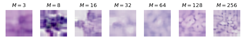
(a) $\mathcal{S}$-VAE

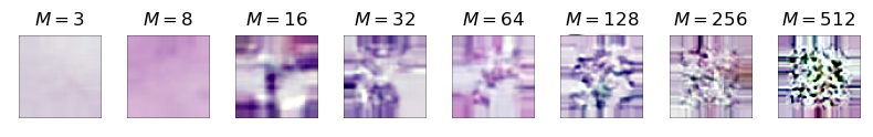
(b) $\mathcal{S}$-AE

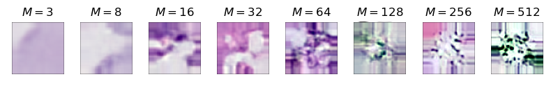
(c) $\mathcal{N}$-VAE

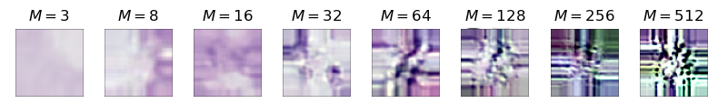
(d) $\mathcal{N}$-AE

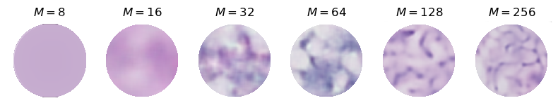
(e) Equivariant $\mathcal{S}$-VAE

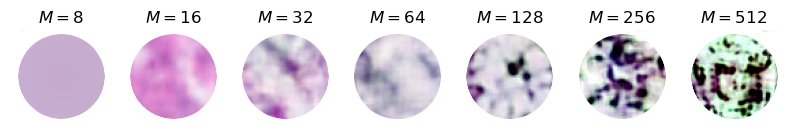
(f) Equivariant $\mathcal{S}$-AE

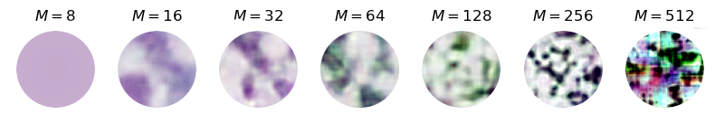
(g) Equivariant $\mathcal{N}$-VAE

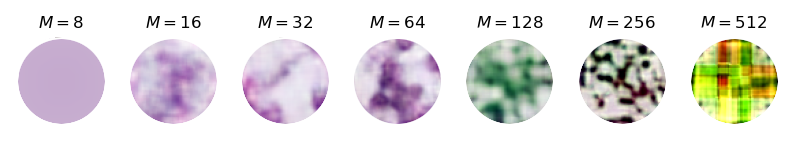
(h) Equivariant $\mathcal{N}$-AE

Figure 5.2: Randomly generated images from all model types. Each column shows one sample from a model trained with a specific latent dimension size.

When comparing the generated images, one trend that is noticeable for almost all models, is that the images decrease in quality for higher dimension sizes. In lower dimensions such as 3, 8 and 16, images are mostly consistent with the appearance of reconstructions, that is, rough blurry shapes with little amount of detail. In higher dimensions, however, images start becoming less realistic, shapes are lost, and colors start appearing that are not originally present in the dataset. This effect seems amplified in equivariant models, most notably the normal vanilla autoencoder, that only produces noise in the highest dimensions. The only model types that do generate realistic images in higher dimensions, that are consistent with reconstructions, are the spherical VAE and its equivariant counterpart. Between these two models, equivariant $\mathcal{S}$-VAE shows slightly more structures that resemble the biopsy patches.

5.3.2.  Interpolations

Next, we discuss the results of the interpolation experiments. For these experiments, one notable finding was that on average, interpolations were of higher quality than randomly generated images. All models, including normal types and autoencoders, produced interpolations that looked smooth, although some differences between models were also observed. First of all, interpolations of spherical-type models were often slightly more realistic in terms of structure than those of normal model types. Examples of this are shown in Figure 5.3. On each row in this figure, six images along the curve between image 1 and image 2 are decoded, including the start and end points, meaning that the second and seventh images are the reconstructions of the original input. Along the interpolation, we see image 1 slowly changing into image 2.

(a)

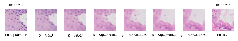
(b)

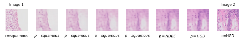
(c)

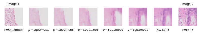
(d)

Figure 5.3: Interpolations of $\mathcal{S}$-VAE and $\mathcal{N}$-VAE models for a latent dimension size of 256. Original input images are shown on the far left and right. Next to each of the original images is their reconstructed version and in the middle of these, the four interpolated images. For the original images, their true class ($c$) is given, while for the other images, the predicted class ($p$) is shown.

For the first interpolation made with $\mathcal{N}$-VAE , as shown in Figure 5.3(a), this transition is more fade-like, and we gradually see more parts of image 2 appearing in the interpolated images and features of image 1 slowly becoming less opaque. Comparing this to the same interpolation made by $\mathcal{S}$-VAE , shown in 5.3(b), however, we can see that the white shape of image 2 is recovered earlier in the interpolation already. Instead of seeing two images fading into each other, we see the shape and structure changing. The same can also be observed in Figures 5.3(c) and 5.3(d). Here too, structures are more noticeable along the interpolation, making them more true to real-life progression than normal type models.

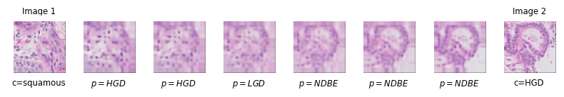
(a)

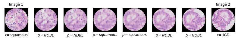
(b)

Figure 5.4: Interpolations of $\mathcal{N}$-VAE and equivariant $\mathcal{N}$-VAE models for a latent dimension size of 512. The equivariant model produces clearer, more structured interpolations.

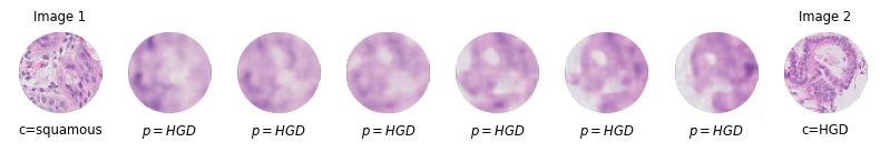
(a)

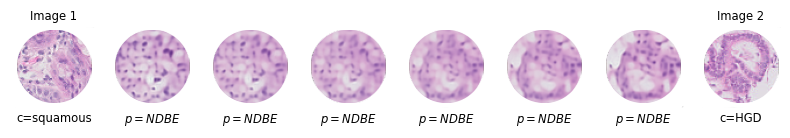
(b)

Figure 5.5: Interpolations of equivariant $\mathcal{N}$-AE and equivariant $\mathcal{S}$-AE models for a latent dimension size of 512. Spherical autoencoders produce clear-looking results, unlike the more blurry interpolations of the normal type autoencoder.

Furthermore, we observe that the roto-equivariant model types produce visually higher quality interpolations than their non-equivariant versions. This becomes especially apparent in normal-type VAEs. An example of this is shown in Figure 5.4, but to a lesser extent in spherical VAEs. Moreover, normal autoencoders, both equivariant and non-equivariant, produce the lowest quality results, with interpolations generally having a blurry appearance, while spherical autoencoders do not suffer from this issue. An example of this is shown in Figure 5.5.

Finally, we also show predicted classes for each of the interpolated images. As became apparent in Subsection 5.2, higher dimensional models, such as 256 and 512, did not achieve good results on the latent representation classification task. Class predictions included in earlier figures are therefore not reliable. For spherical models of dimension 32 however, accuracy scores were on average higher. We therefore include an example of an interpolation made by $\mathcal{S}$-VAE with size 32 in Figure 5.6. In this figure, it can be seen that, although the image quality is more blurry, predicted classes for images 1 and 2 are correct. A shift from squamous tissue to the first stage of Barrett’s esophagus, NDBE, occurs towards the end of the interpolation, which ends at high-grade dysplasia.

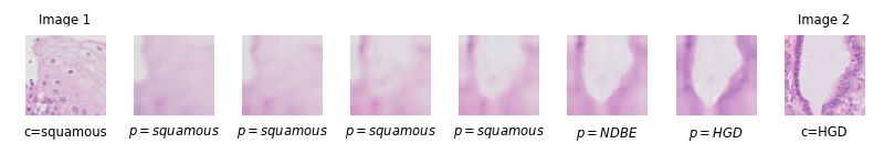
Figure 5.6: Interpolation between squamous and high-grade dysplasia by model with latent dimension size of $M=32$. Although the quality of images is lower, the predicted classes are correct and show a more realistic progression.

5.4. Spherical Autoencoder as Generative Model

5.4.1.  Random Sampling with Spread Loss

Finally, to evaluate our novel $\mathcal{S}$-AE model and determine its potential as a generative model, we examine the effects of spread loss on the spherical autoencoder model. First and most importantly, we evaluate the quality of randomly generated images, as this will make clear if the model with spread loss can be used for generative tasks. To compare how spread loss affects models differently, we also provide samples generated by a variational spherical autoencoder trained with spread loss.

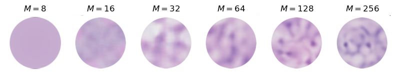
(a) Equivariant $\mathcal{S}$-VAE model with Spread Loss

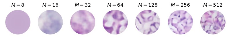
(b) Equivariant $\mathcal{S}$-AE model with Spread Loss

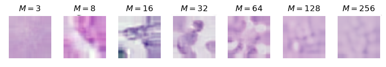
(c) $\mathcal{S}$-VAE model with Spread Loss

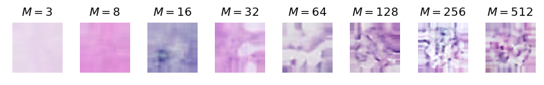
(d) $\mathcal{S}$-AE model with Spread Loss

Figure 5.7: Randomly image samples generated by $\mathcal{S}$-VAE and $\mathcal{S}$-AE with spread Loss, for a range of latent dimension sizes.

In Figure B.19, we show one sample per dimension size of all spherical models with spread loss implemented. As can be observed from this figure, the visual quality of the images generated by the spherical autoencoder model types greatly improves compared to samples generated by the same models without spread loss (Figure 5.2. The images look more realistic and continue to do so up until the highest tested dimension sizes. This effect is most noticeable for the equivariant $\mathcal{S}$-AE model. For the variational models, spread loss does not have a large effect on the quality of samples, except for the images being slightly less sharp than before.

Furthermore, when interpolating with models with spread loss, we do not see a noticeable improvement. This may be explained due to spherical autoencoders already generating good-quality interpolations without the extra loss function. In some rare cases, interpolations with spread loss result in low-quality images, such as the ones shown in Figure 5.8. Here, interpolations do not model a smooth transition, suggesting that the spreading of encoded points can create some low-information areas in the latent space. This most commonly occurs in higher latent dimensions.

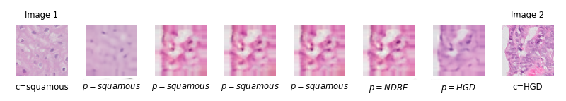
Figure 5.8: Interpolation generated by $\mathcal{S}$-AE model with spread loss and $M=512$. The interpolation does not appear smooth.

5.4.2.  Effects of Spread Loss on Quantitative Metrics

Finally, having demonstrated the potential of the spherical autoencoder with spread loss as a generative model, we test if the extra loss function has a negative impact on quantitative measures by evaluating the performance on reconstruction loss and classification accuracy. Table 5.4 shows the reconstruction losses earlier reported for the original autoencoder models on the left and the new loss values for the spread loss autoencoders on the right. It can be observed that spread loss does not have an adverse effect on reconstruction error, with the exception of the largest dimension sizes of 256 and 512. Across all other latent dimension sizes, spread loss actually shows improved performance over their models’ original versions.

Table 5.4: Effect of Spread Loss on Reconstruction Error

	Original		Spread Loss
$M$	$\mathcal{S}$-AE	Eq. $\mathcal{S}$-AE	$\mathcal{S}$-AE	Eq. $\mathcal{S}$-AE
$3$	2089.98	-	1881.539	-
$8$	1743.25	2103.27	1712.125	2102.35
$16$	1607.79	1313.58	1539.761	1271.64
$32$	1403.93	1135.50	1379.716	1139.093
$64$	1258.50	992.39	1226.048	1004.461
$128$	1104.18	853.75	1087.761	874.803
$256$	925.07	703.88	956.545	757.036
$512$	727.06	540.13	877.659	624.188

Table 5.5: Effect of Spread Loss on Classification Accuracy

	Original		Spread Loss
$M$	$\mathcal{S}$-AE	Eq. $\mathcal{S}$-AE	$\mathcal{S}$-AE	Eq. $\mathcal{S}$-AE
$3$	0.262	-	0.262	-
$8$	0.325	0.274	0.326	0.198
$16$	0.343	0.298	0.344	0.290
$32$	0.308	0.455	0.308	0.250
$64$	0.409	0.433	0.413	0.283
$128$	0.393	0.282	0.325	0.361
$256$	0.406	0.243	0.430	0.315
$512$	0.371	0.254	0.454	0.422

Additionally, Table 5.5 shows the test accuracies on the latent representation classification task for both original and spread loss autoencoders. For non-equivariant autoencoders, the accuracy scores obtained with spread loss are very comparable to the original scores. The only exceptions are the higher dimensions, 256 and 512, where the model with spread loss achieves a higher accuracy than the original $\mathcal{S}$-AE . Notably, this is the opposite pattern of the reconstruction losses, as the highest two dimensions score the worst there. For equivariant autoencoders, a different pattern can be observed. Before, a latent dimension size of 32 scored the highest, but here, that same model with spread loss scores is one of the lowest out of all dimension sizes. Instead, the best scoring size is the highest dimension size, 512.

Section 6. Discussion

In this final section, we will discuss the results reported in Section 5 and provide a conclusion for the experiments. Section 6.1 will include the analysis of the results, Section 6.2 will discuss some limitations and possibilities for future work, and Section 6.3 will summarize this work and provide the concluding remarks.

6.1. Analysis of Results

To determine the potential of spherical models for learning meaningful histopathological representations, we first start by discussing the experiments for non-equivariant variational autoencoders and later discuss the effects of adding rotation-disentanglement to these models. Consequently, special attention is given to the non-variational framework, and we discuss the results for our own generative $\mathcal{S}$-AE model.

6.1.1.  Evaluation of Spherical and Normal-Type VAEs

Reconstruction Error

To start, during the reconstruction experiments, we observed that spherical models produce better quality reconstructions than normal-type VAEs in lower latent dimension sizes, but not in higher dimensions. This is in line with the work of Davidson et al., as the authors there also describe that their model is limited in higher dimension sizes. In lower dimensions, the uniform prior allows for a natural form of encoding and clustering, and the model is able to use the entire compact space of the hyperspherical surface. This improves performance over normal-type models that use a Gaussian prior, as is reflected in the reconstruction losses. However, as dimensionality increases, the surface area starts to vanish, which limits the possible space for the model to encode points on, as was described in subsection 4.2.2. Although this numerical instability initially limited the model to latent dimensions sizes of less than 20, we found that restricting the concentration parameter $\kappa$ had a positive effect on stability, allowing the spherical VAEs to be trained up to and including a latent size of 256. Nevertheless, it should be noted that, as $\kappa$ is fixed for all dimensions, the expressivity of the spherical VAE naturally decreases the higher the dimensionality becomes. Therefore, combining our modification of $\kappa$ with the already restricted nature of the vMF distribution in high dimensions could potentially decrease model expressivity by a great amount compared to normal-type models. These two limitations of spherical VAEs could explain how normal-type VAEs outperform the spherical models for higher dimension sizes in the reconstruction loss results.

Classifiability

A similar trend was observed during the classification experiments. Here, spherical VAEs outperformed normal types in the lower dimensions 3-32, but not in the higher range of 64-256. On average, the highest scores on the latent representation classification task were not far behind those of the CNN directly classifying the patches. The $\mathcal{N}$-VAE model, for instance, reached 0.454 for a latent dimension of 64, while the CNN model reached 0.450 in these same settings. This is perhaps surprising, as state-of-the-art deep learning for the classification of Barrett’s esophagus has often reached 0.8 to 0.9 accuracy on test datasets Hussein et al. (2022); Hong et al. (2017). One reason as to why the current CNNs do not reach this level of performance may be the size of the patches, or more specifically, the amount of information present in them. Unlike VAEs, CNN classifiers generally use a much larger patch size, such as 512$\times$512 with a magnification of 10$\times$, which provides both more detail and more information. In comparison, the patch size used in the current experiments, 64$\times$64 with a magnification of 5$\times$, provides four times less the amount of context. This can be an essential factor in determining the classifiability of the patches, as well as their encoded latent representations. Although not all the required information needed to reach a high accuracy score may be present in the patches, the classification experiments do show that there is a minimal loss of information between the patches and their lower-dimensional representations, suggesting that the models are able to learn an encoding that is meaningful within these settings.

Generative Quality

Furthermore, comparing the spherical VAEs to the normal VAEs for the qualitative experiments, we see a clear improvement across the entire tested dimensionality range. When using $\mathcal{S}$-VAE and $\mathcal{N}$-VAE to randomly generate new images, the normal VAE produces noisy images from a dimension size of 32 upwards, while the spherical model produces realistic output up until the largest dimension size. The lackluster quality of the normal-type VAE in higher dimensions might possibly be attributed to the fixing of the variance parameter to an isotropic scalar value. This was done to be able to compare the architecture to the spherical model, and to fairly assess the effects of roto-equivariance on the model. However, it may also lead to decreased model expressivity in higher-dimensional settings. Further experiments would be needed to confirm this hypothesis. For $\mathcal{S}$-VAE , we observed that as dimensionality increases, general shapes in the generated images start to become more fine-grained. In the highest dimension ranges, $\mathcal{S}$-VAE generates images that contain much more detail than lower-dimensional images, but the generations also contain relatively more blurriness, less clear structures and less color variation than the reconstructions for those dimension sizes. Conversely, images generated by $\mathcal{S}$-VAE latent dimensions 16 and 32, do resemble their corresponding reconstructions to a greater extent. The reduction of generation quality in higher dimensions can therefore again be explained due to the decreased model expressivity, and the decreasing surface area to encode the images on in that dimensionality range. The decreased performance in high dimensions of spherical models does not become apparent during the interpolation experiments. There, across all dimensionalities, $\mathcal{S}$-VAE shows a slight improvement in interpolation quality over $\mathcal{N}$-VAE , that is mainly noticeable in the better retainment of shape and structure.

6.1.2.  The Effects of Rotation-Disentanglement

Rotation-Disentanglement Improves Allover Performance

Another interesting finding is that the addition of roto-equivariance to the spherical setting generally increased performance across all experiments. Especially in medium to high range of dimension sizes (from 16 upwards), equivariant models improved reconstruction loss, classification accuracy and quality of generated images and interpolations over their not roto-equivariant versions. A similar trend was also observed for the $\mathcal{N}$-VAE , but the effect of equivariance did not become as apparent as in the hyperspherical case. It is possible that the positive effects of spherical and roto-equivariant techniques amplify each other. The roto-equivariance allows the model to learn a rotation-disentangled representation, and because of the absence of unnecessary information in this representation, it becomes easier to encode on the latent space. The improved structuring of this space in the hyperspherical setting could then improve the quality of the representations even further, leading to an improved benefit of the roto-equivariance in spherical settings compared to normal settings.

Spherical VAEs learn a more meaningful representation in lower dimensions

Considering the abovementioned improved performance across all experiments for spherical VAEs, and their potential to be even further improved by the addition of roto-equivariance, the results suggest that spherical models learn representations that are more meaningful than those of the vanilla VAE, but that they may be better used in low-dimensional settings. However, this brings us to the bottleneck central to this work. Spherical models are limited to a lower dimension range, but the histopathological image patches that these model are applied to, are too complex to be accurately encoded and recovered using a lower latent dimension. This became apparent from for instance Figure 5.1. It was observed that even the highest latent dimension sizes still do not recover the original image completely accurately, suggesting that the latent dimension should at least be 512 or higher to obtain a good reconstruction. Additionally, it is likely that classifications of both representations as well as direct patch classification will improve by using patches that cover a larger biopsy area. However, the additional context and detail could make it even harder for the models to learn good encodings in low-dimensional settings, therefore also requiring a high latent dimension size. With the current setting for $\mathcal{S}$-VAE , such a larger patch size would be very difficult to process.

6.1.3.  Spherical Autoencoders

We therefore introduced spherical autoencoders as a possible alternative to $\mathcal{S}$-VAE , and included non-variational versions of each model in the experiments. As mentioned in 4.2.2, spherical autoencoders did not show the same numerical instability as variational spherical autoencoders and were therefore applicable to higher dimensionalities. Moreover, autoencoders are known to produce sharper reconstructions than variational models, suggesting their potential for improving quantitative results.

Autoencoders Obtain Lower Reconstruction Errors

For the reconstruction experiments, it was shown that the autoencoder version of every model, both equivariant and non-equivariant, achieved a lower reconstruction error on the test set in higher dimensions. This was especially apparent for the spherical models. The observations are therefore in line with earlier work stating that variational autoencoders generally produce less sharp reconstructions than their non-variational counterparts. Moreover, the classification experiments showed no notable reduction in the classifiability of the learned latent representations. Although autoencoders showed an improvement in the quantitative experiments, they did not compare to the spherical variational models during the qualitative analysis of generated images. Here, it became apparent that autoencoders are often not considered as a generative model, as the models could only produce non-realistic noisy images in the majority of the tested dimensionality range. Interpolations generated by the spherical autoencoder did however show a vast improvement of quality over the vanilla autoencoder model, suggesting that the spherical structuring of the latent space provided a benefit to the learned representations in the non-variational case as well.

Spread Loss Improves the Quality of $\mathcal{S}$-AE ’s Generations

Therefore, the spread loss function was introduced and applied to the spherical autoencoder, and examples of generated images were provided for this modified architecture. In these experiments, it was shown that the addition of spread loss substantially impacted the quality of the generated images in a positive way. Where spherical autoencoders could only generate noise before, the sampled images now resembled those generated by $\mathcal{S}$-VAE . We suspect that in the original $\mathcal{S}$-AE , images were often encoded close together, in a relatively small area on the hyperspherical surface, and that the amount of unutilized space only grew in larger dimensions. This would explain why randomly sampled images appeared as noise: the greater the dimension of the latent hypersphere, the more likely it would become that random images were sampled from an empty, uninformed location on the surface.

Furthermore, this would also be in line with the interpolation experiments, in which we showed that non-modified $\mathcal{S}$-AE models, contrary to generative random sampling, produced good-quality interpolations over all dimensions. The encoded points all being clustered in a specific area of the hypersphere would mean they are close together and allow for smooth interpolations. Finally, a similar phenomenon was observed in the visualizations of the hyperspherical latent space in 3D, as we could see that the encoded points covered mainly one side of the sphere; an effect that would only increase the higher the latent size becomes according to this hypothesis. Encouraging the encodings to be spread uniformly over the sphere through the spread loss, which in the variational setting is accomplished by the prior, would therefore decrease the amount of empty surface area. This in turn is then hypothesized to lead to the improved random sampling observed in Subsection 5.4.1, but also the more unstable, less smooth interpolations that sometimes occurred.

Quantitative Results with Spread Loss are Comparable to Regular $\mathcal{S}$-AE

Quantitative experiments were also conducted on models with spread loss, and these showed no substantial negative effects of the modified loss function on reconstruction loss or classification accuracy. Even more so, the spread loss model demonstrated an improved accuracy in dimensions 256 and 512, which may perhaps be explained by the spread making it easier for a classifier to differentiate the otherwise closely clustered points. Although this work only provides an initial step, the experiments with spread loss show a potential for the proposed $\mathcal{S}$-AE to be used as a generative model, which would make it a promising alternative to $\mathcal{S}$-VAE in higher dimensions.

6.2. Limitations and Future Work

As mentioned in the discussion of the results, one of the greatest limitations of this work was the fact that the models, especially $\mathcal{S}$-VAE , had trouble performing in higher dimensions, while the patches required higher latent dimensions to be accurately encoded and decoded. Future work could therefore focus on either one of these limiting factors, or a combination of both.

6.2.1.  Experimenting with Patches

Patch Size

In regards to improving the ability of the models to process the images, we could for instance experiment with different sizes and magnification levels of patches. Lafarge et al. for example, use a high magnification level, showing only one cell per image patch, and are able to successfully use $\mathcal{N}$-VAE and the roto-equivariant $\mathcal{N}$-VAE to create high-quality reconstructions using a latent dimension size of 64. While our goal of modeling cell progression on a higher, tissue-based level would require a patch to contain more context than just one cell, the results of Lafarge et al. do show that a higher magnification level, or rather a higher resolution image, might be easier for VAEs to reconstruct. This was also confirmed in earlier work by for example Thambawita et al. (2021). We could therefore start experimenting with using a magnification level of 10$\times$ and a patch size of 128$\times$128. This would correspond to the same amount of biopsy area per patch as in the original experiments, but with a higher resolution. Although initial experiments showed that patches of this size were more difficult for the model to computationally process, experimenting with hyperparameters such as batch size and learning rate might alleviate this issue. Experimenting with such patches could show if the higher resolution does indeed have a positive effect on reconstruction quality, and if so, if a lower latent dimension size would be sufficient. Following Thambawita et al., classification of patches might also be improved by using a higher image resolution, as a size of 512$\times$512 with a 10$\times$ magnification seems to be the standard Hong et al. (2017); Thambawita et al. (2021). Further experiments could clarify if the models can be extended to process even larger patch sizes.

Patch Labels

Besides patch size, classification might also be improved by considering alternative labeling systems. In this work, labels were assigned based on the most dominant pixel value present in a patch, and this was the only technique that was considered. Alternative labeling methods exist that do not consider the dominant pixel, but the value of the pixel in the middle of a patch Li et al. (2022). It would be interesting to determine the effects of another labeling method on the assigned patch classes. For example, currently over 60% of the patches were labeled as NDBE, which lead us to discard part of these patches from the training dataset. Another labeling technique could produce a different, more balanced distribution of classes, and although the results showed no obvious signs of a shortage of training data, this would result in an additional number of patches that could be included in the dataset. Furthermore, as a side note, it is also possible that the Vienna criteria class system in general is not a good fit for the data. As VAEs learn in an unsupervised manner, there is no guarantee that they cluster the encodings on the latent space in the four classes used in this work. Classification into such categories might in that case be difficult. The Vienna criteria have been used in clinical practice and have been used to train successful deep-learning classifiers, so it is probable that the class system is a satisfactory fit for the problem of modeling BE progression. However, should research on latent representation learning for BE advance, then it would be desirable that the utility of the class system is tested, for example by training a model such as K-means clustering on the latent space and seeing what the optimal number of clusters is.

6.2.2.  Improving Models

Improving $\mathcal{S}$-VAE in Higher Dimensions

On the other hand, future research could also focus on improving $\mathcal{S}$-VAE in higher dimensions. An extension of the original paper by Davidson et al. was introduced that aimed to increase the expressivity of the model in higher dimensions by introducing additional concentration parameters Davidson et al. (2019). This reduced the limiting effects of $\kappa$ being fixed for all dimensionalities. Such a method could also be implemented for the current use case, however, the problem of numerical instability would still persist. We took a first step towards showing the potential of $\mathcal{S}$-AE as a generative model and a more stable alternative to $\mathcal{S}$-VAE in higher dimensions. Although results showed promise, we believe many experiments would need to be conducted before $\mathcal{S}$-AE can be called a true competitor to $\mathcal{S}$-VAE . First and foremost, $\mathcal{S}$-AE should be applied to a simpler problem so that a proof of concept can be made. A first step would therefore be to apply the model to for example the MNIST dataset. If results remain promising on this dataset, extensions to more complicated datasets can be made. In a histopathological setting, it would for example be interesting to test both $\mathcal{S}$-AE and $\mathcal{S}$-VAE on a simpler progression modeling task that requires a lower dimension to accurately reconstruct and is easier to cluster and classify, such as healthy tissue to dysplasia or to cancer. Not only could we better test the potential of spherical models for modeling morphological tissue changes in general, but we would also better be able to study the possible limitations and benefits of spherical autoencoders.

Extending RHVAE to Larger Datasets

Finally, experiments with the Riemannian model RHVAE were halted by the model being unable to scale to larger training datasets, and we instead focused our efforts on the spherical models for the further part of this work. The concept of Riemannian latent space structuring itself could still be an interesting alternative to $\mathcal{S}$-VAE however. For example, we showed that in initial experiments with default settings, the model was already able to create latent space in which data points belonging to squamous tissue and high-graded dysplasia were clustered. Moreover, we also observed that the quality of reconstructions and generated samples was closer to that of the original input images, showing more intricate tissue patterns than spherical and normal-type models. These preliminary results indicate that the Riemannian latent space modeling could be a good choice for histopathological data and should be investigated in future work. The main hurdle to overcome in that case, is to make it feasible for the Riemannian VAE to process a large dataset becomes. One possible approach to accomplish this is by exploring alternative methods of learning the Riemannian metric, such that is not parameterized by all data points. Some ideas regarding efficient metric learning were for example proposed by Louis et al. (2019) and Gruffaz et al. (2021). Alternatively, the learning of the metric might at all be unnecessary if we can directly compute it in a computationally efficient way, such as attempted by Jeong et al. (2021) or Fan et al. (2022).

6.3. Conclusion

In this work, we studied how the latent space of a VAE could be geometrically structured such that it models the progression of healthy tissue to Barrett’s esophagus. A number of different techniques were researched, most notably RHVAE, which structures the latent space as a Riemannian manifold with a metric learned from the data, and $\mathcal{S}$-VAE , which structures the manifold as a hypersphere on which the beneficial uniform prior can be imposed. Additionally, an extension of $\mathcal{S}$-VAE to a rotation-equivariant group-based architecture was studied. We then asked which of the different manifold topologies, regular Euclidean, Riemannian, or hyperspherical, was the best choice to model disease progression by evaluating the models on four different tasks: reconstruction of input, classifiability of latent representations, quality of randomly generated images, and quality of interpolations. We found that RHVAE unfortunately could not be tested on the current dataset, as the model was limited to only small-scale datasets.

Between the vanilla $\mathcal{N}$-VAE and hyperspherical $\mathcal{S}$-VAE , the results showed that spherical models had improved performance over vanilla VAEs, especially in lower-dimensional settings. Here, they obtained better reconstruction errors than normal-type VAEs and their representations were shown to be easier for a simple linear model to classify. Moreover, they consistently generated high-quality image samples, even in higher dimensions where other models could only generate noise. Furthermore, their interpolations were more true to real-life changes in cell tissue. Additionally, the roto-equivariant version of the spherical models improved their performance even more across all evaluated tasks, which further established their potential for learning meaningful representations.

However, we also showed that the spherical VAEs were unable to perform in higher dimensions, showing limited expressivity and severe numerical instability issues. This posed a problem for histopathological images, as they contain many fine-grained details and are hard to reconstruct in low dimensions accurately. We therefore investigated non-variational spherical autoencoders and showed that they achieved lower reconstruction errors than variational models, and were less numerically unstable, allowing them to reach the higher dimensions the histopathological images require. We furthermore proposed to solve their inability to generate realistic random images by introducing spread loss and showed that this custom loss function could be used to significantly improve the quality of generations by spherical autoencoders, while having minimal to no impact on reconstruction quality or classifiability.

Even with these improved results, a certain degree of blurriness remained in the reconstructions, and generated samples of all model types were still not on par with the quality of the original patches. Although we demonstrated several benefits of geometric-inspired VAEs over regular VAEs, the results suggest that the latent space learned by these models does not yet have the desired data-supporting structure to be able to model the progression of BE, and that some steps toward this goal remain to be made. On a short-term basis, experiments with different preprocessing of patches could make it easier for models to represent their features in the latent space. In the longer term, it would be desirable to look into alternative geometric-inspired models that do not suffer from the same issues as $\mathcal{S}$-VAE in higher dimensions. Although more experiments would be needed to determine its full potential, the initial results described in this work suggest that our $\mathcal{S}$-AE model could potentially form one such promising alternative to $\mathcal{S}$-VAE , both in this histopathological setting and in other applications.

Appendix A Model Architectures

A.1. Non-Equivariant Network Architecture

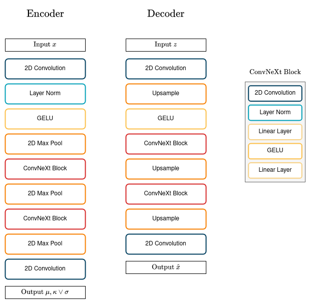
Figure A.1: Architecture of non-equivariant spherical and normal-type models. All convolutions use a kernel size of 5 and all pooling operations use a size and stride of 2. A padding of size 4 is added to the decoder network’s convolutions. The ConvNeXt blocks implement a point wise convolution through linear layers.

A.2. Equivariant Network Architecture

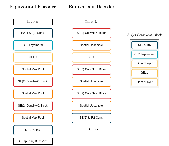
Figure A.2: Architecture of non-equivariant spherical and normal-type models. The same parameters apply as for the non-equivariant network version.

Appendix B Extended Results

B.1. Reconstruction Losses

Model	Reconstruction Loss
	Training Set	Validation Set	Test Set
Eq. $\mathcal{N}$-AE	-	-	-
Eq. $\mathcal{N}$-VAE	-	-	-
Eq. $\mathcal{S}$-AE	-	-	-
Eq. $\mathcal{S}$-VAE	-	-	-
$\mathcal{N}$-AE	1959.97	2013.46	2013.46
$\mathcal{N}$-VAE	1985.43	1895.84	1895.56
$\mathcal{S}$-AE	2008.79	2089.97	2089.98
$\mathcal{S}$-VAE	1927.77	1931.04	1930.60

(a) Reconstruction Losses for $M=3$

Model	Reconstruction Loss
	Training Set	Validation Set	Test Set
Eq. $\mathcal{N}$-AE	2357.94	2103.35	2103.35
Eq. $\mathcal{N}$-VAE	2357.97	2103.47	2103.47
Eq. $\mathcal{S}$-AE	2357.93	2103.27	2103.27
Eq. $\mathcal{S}$-VAE	2070.93	2103.66	2103.66
$\mathcal{N}$-AE	1772.95	1769.14	1769.14
$\mathcal{N}$-VAE	1803.51	1807.24	1807.06
$\mathcal{S}$-AE	1791.27	1743.26	1743.25
$\mathcal{S}$-VAE	1428.10	1706.56	1707.14

(b) Reconstruction Losses for $M=8$

Model	Reconstruction Loss
	Training Set	Validation Set	Test Set
Eq. $\mathcal{N}$-AE	1434.19	1252.64	1252.64
Eq. $\mathcal{N}$-VAE	1498.07	1290.29	1290.60
Eq. $\mathcal{S}$-AE	1449.96	1313.59	1313.58
Eq. $\mathcal{S}$-VAE	1336.07	1303.61	1303.07
$\mathcal{N}$-AE	1677.37	1621.97	1621.97
$\mathcal{N}$-VAE	1701.18	1635.89	1635.89
$\mathcal{S}$-AE	1687.61	1607.79	1607.79
$\mathcal{S}$-VAE	1695.08	1562.78	1563.19

(a) Reconstruction Losses for $M=16$

Model	Reconstruction Loss
	Training Set	Validation Set	Test Set
Eq. $\mathcal{N}$-AE	1316.68	1134.30	1134.30
Eq. $\mathcal{N}$-VAE	1316.84	1161.32	1161.32
Eq. $\mathcal{S}$-AE	1313.97	1135.50	1135.50
Eq. $\mathcal{S}$-VAE	1276.09	1142.35	1142.24
$\mathcal{N}$-AE	1392.95	1273.44	1273.44
$\mathcal{N}$-VAE	1237.93	1092.88	1092.88
$\mathcal{S}$-AE	1398.56	1258.50	1258.50
$\mathcal{S}$-VAE	1317.13	1389.48	1389.64

(b) Reconstruction Losses for $M=32$

Model	Reconstruction Loss
	Training Set	Validation Set	Test Set
Eq. $\mathcal{N}$-AE	1162.61	988.42	988.42
Eq. $\mathcal{N}$-VAE	1175.99	993.96	993.94
Eq. $\mathcal{S}$-AE	1173.26	992.39	992.39
Eq. $\mathcal{S}$-VAE	1067.34	1009.92	1009.90
$\mathcal{N}$-AE	1392.95	1273.44	1273.44
$\mathcal{N}$-VAE	1408.42	1260.84	1260.85
$\mathcal{S}$-AE	1398.56	1258.50	1258.50
$\mathcal{S}$-VAE	1547.71	1250.33	1250.45

(a)

Model	Reconstruction Loss
	Training Set	Validation Set	Test Set
Eq. $\mathcal{N}$-AE	1007.24	853.79	853.79
Eq. $\mathcal{N}$-VAE	1015.57	857.40	857.40
Eq. $\mathcal{S}$-AE	1012.55	853.76	853.75
Eq. $\mathcal{S}$-VAE	1125.63	902.90	902.82
$\mathcal{N}$-AE	1224.29	1113.56	1113.56
$\mathcal{N}$-VAE	1237.93	1092.88	1092.88
$\mathcal{S}$-AE	1223.13	1104.18	1104.18
$\mathcal{S}$-VAE	1321.64	1133.48	1133.33

(b)

Model	Reconstruction Loss
	Training Set	Validation Set	Test Set
Eq. $\mathcal{N}$-AE	807.57	706.50	706.50
Eq. $\mathcal{N}$-VAE	817.84	710.25	710.22
Eq. $\mathcal{S}$-AE	812.39	703.88	703.88
Eq. $\mathcal{S}$-VAE	981.48	826.55	826.10
$\mathcal{N}$-AE	1021.52	935.09	935.09
$\mathcal{N}$-VAE	1046.39	904.53	904.53
$\mathcal{S}$-AE	1022.95	925.07	925.07
$\mathcal{S}$-VAE	1147.48	1056.91	1056.68

(a)

Model	Reconstruction Loss
	Training Set	Validation Set	Test Set
Eq. $\mathcal{N}$-AE	599.36	556.61	556.61
Eq. $\mathcal{N}$-VAE	611.42	562.07	562.11
Eq. $\mathcal{S}$-AE	585.31	540.13	540.13
Eq. $\mathcal{S}$-VAE	-	-	-
$\mathcal{N}$-AE	804.67	736.92	736.92
$\mathcal{N}$-VAE	851.73	748.40	748.42
$\mathcal{S}$-AE	801.83	727.06	727.06
$\mathcal{S}$-VAE	-	-	-

(b)

B.2. Classification Accuracies

Model	Classification Accuracy
	Training Set	Validation Set	Test Set
Eq. $\mathcal{N}$-AE	-	-	-
Eq. $\mathcal{N}$-VAE	-	-	-
Eq. $\mathcal{S}$-AE	-	-	-
Eq. $\mathcal{S}$-VAE	-	-	-
$\mathcal{N}$-AE	0.55	0.25	0.25
$\mathcal{N}$-VAE	0.41	0.25	0.25
$\mathcal{S}$-AE	0.48	0.25	0.25
$\mathcal{S}$-VAE	0.38	0.26	0.26

(a)

Model	Classification Accuracy
	Training Set	Validation Set	Test Set
Eq. $\mathcal{N}$-AE	0.20	0.14	0.14
Eq. $\mathcal{N}$-VAE	0.22	0.27	0.27
Eq. $\mathcal{S}$-AE	0.45	0.27	0.27
Eq. $\mathcal{S}$-VAE	0.38	0.23	0.23
$\mathcal{N}$-AE	0.50	0.35	0.35
$\mathcal{N}$-VAE	0.58	0.33	0.33
$\mathcal{S}$-AE	0.55	0.36	0.36
$\mathcal{S}$-VAE	0.41	0.35	0.35

(b)

Model	Classification Accuracy
	Training Set	Validation Set	Test Set
Eq. $\mathcal{N}$-AE	0.59	0.42	0.42
Eq. $\mathcal{N}$-VAE	0.55	0.38	0.38
Eq. $\mathcal{S}$-AE	0.52	0.30	0.30
Eq. $\mathcal{S}$-VAE	0.42	0.34	0.34
$\mathcal{N}$-AE	0.59	0.40	0.40
$\mathcal{N}$-VAE	0.67	0.38	0.38
$\mathcal{S}$-AE	0.61	0.39	0.39
$\mathcal{S}$-VAE	0.56	0.40	0.40

(a)

Model	Classification Accuracy
	Training Set	Validation Set	Test Set
Eq. $\mathcal{N}$-AE	0.61	0.45	0.45
Eq. $\mathcal{N}$-VAE	0.61	0.45	0.45
Eq. $\mathcal{S}$-AE	0.64	0.45	0.45
Eq. $\mathcal{S}$-VAE	0.47	0.48	0.48
$\mathcal{N}$-AE	0.69	0.38	0.38
$\mathcal{N}$-VAE	0.64	0.39	0.39
$\mathcal{S}$-AE	0.69	0.42	0.42
$\mathcal{S}$-VAE	0.47	0.41	0.41

(b)

Model	Classification Accuracy
	Training Set	Validation Set	Test Set
Eq. $\mathcal{N}$-AE	0.63	0.43	0.43
Eq. $\mathcal{N}$-VAE	0.66	0.39	0.39
Eq. $\mathcal{S}$-AE	0.59	0.43	0.43
Eq. $\mathcal{S}$-VAE	0.77	0.39	0.39
$\mathcal{N}$-AE	0.67	0.40	0.40
$\mathcal{N}$-VAE	0.61	0.42	0.42
$\mathcal{S}$-AE	0.64	0.38	0.38
$\mathcal{S}$-VAE	0.66	0.40	0.40

(a)

Model	Classification Accuracy
	Training Set	Validation Set	Test Set
Eq. $\mathcal{N}$-AE	0.64	0.39	0.39
Eq. $\mathcal{N}$-VAE	0.67	0.41	0.41
Eq. $\mathcal{S}$-AE	0.64	0.28	0.28
Eq. $\mathcal{S}$-VAE	0.64	0.39	0.39
$\mathcal{N}$-AE	0.72	0.43	0.43
$\mathcal{N}$-VAE	0.72	0.39	0.39
$\mathcal{S}$-AE	0.70	0.36	0.36
$\mathcal{S}$-VAE	0.64	0.41	0.41

(b)

Model	Classification Accuracy
	Training Set	Validation Set	Test Set
Eq. $\mathcal{N}$-AE	0.72	0.39	0.39
Eq. $\mathcal{N}$-VAE	0.70	0.42	0.42
Eq. $\mathcal{S}$-AE	0.50	0.24	0.24
Eq. $\mathcal{S}$-VAE	0.75	0.42	0.42
$\mathcal{N}$-AE	0.83	0.42	0.42
$\mathcal{N}$-VAE	0.83	0.44	0.44
$\mathcal{S}$-AE	0.64	0.37	0.37
$\mathcal{S}$-VAE	0.69	0.42	0.42

(a)

Model	Classification Accuracy
	Training Set	Validation Set	Test Set
Eq. $\mathcal{N}$-AE	0.80	0.38	0.38
Eq. $\mathcal{N}$-VAE	0.88	0.42	0.42
Eq. $\mathcal{S}$-AE	0.52	0.25	0.25
Eq. $\mathcal{S}$-VAE	-	-	-
$\mathcal{N}$-AE	0.83	0.37	0.37
$\mathcal{N}$-VAE	0.89	0.40	0.40
$\mathcal{S}$-AE	0.63	0.29	0.29
$\mathcal{S}$-VAE	-	-	-

(b)

B.3. Generated Samples

Figure B.8: Eight randomly sampled images from Equivariant $\mathcal{S}$-VAE model trained with varying latent dimensions

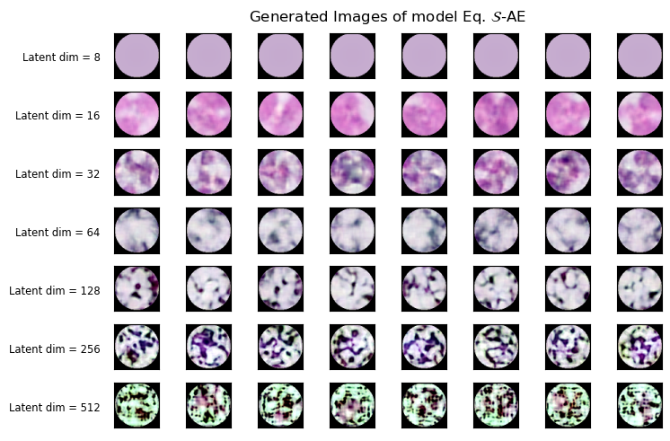
Figure B.9: Eight randomly sampled images from Equivariant $\mathcal{S}$-AE model without spread loss, trained with varying latent dimensions

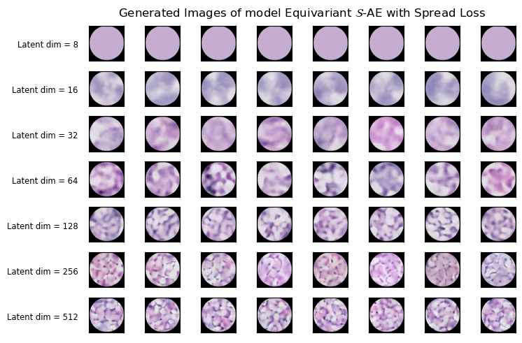
Figure B.10: Eight randomly sampled images from Equivariant $\mathcal{S}$-AE model with spread loss, trained with varying latent dimensions

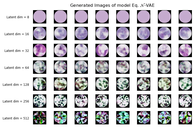
Figure B.11: Eight randomly sampled images from Equivariant $\mathcal{N}$-VAE model trained with varying latent dimensions

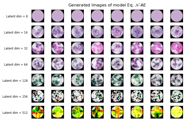
Figure B.12: Eight randomly sampled images from Equivariant $\mathcal{N}$-AE model trained with varying latent dimensions

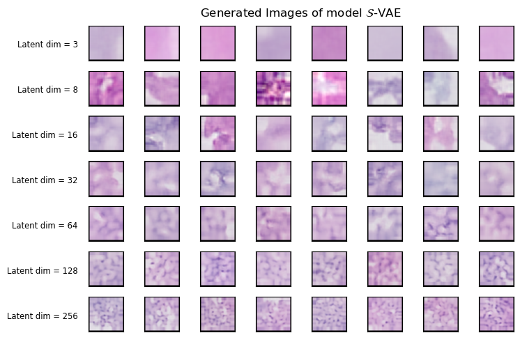
Figure B.13: Eight randomly sampled images from $\mathcal{S}$-VAE model trained with varying latent dimensions

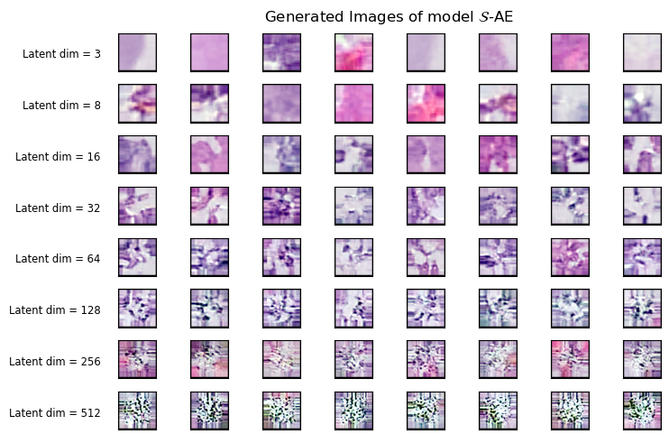
Figure B.14: Eight randomly sampled images from $\mathcal{S}$-AE model without spread loss, trained with varying latent dimensions

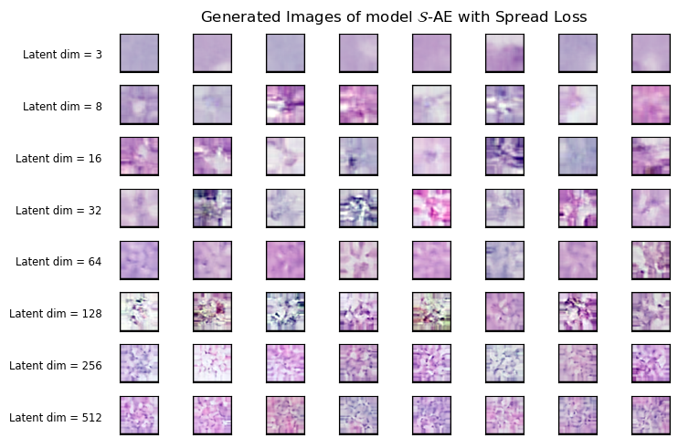
Figure B.15: Eight randomly sampled images from $\mathcal{S}$-AE model with spread loss, trained with varying latent dimensions

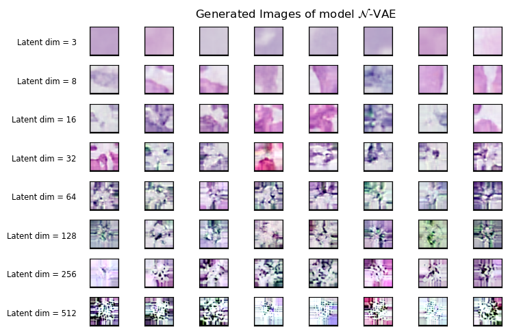
Figure B.16: Eight randomly sampled images from $\mathcal{N}$-VAE model trained with varying latent dimensions

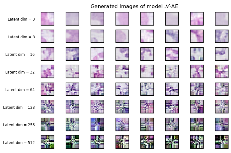
Figure B.17: Eight randomly sampled images from $\mathcal{N}$-AE model trained with varying latent dimensions

B.4. Interpolations

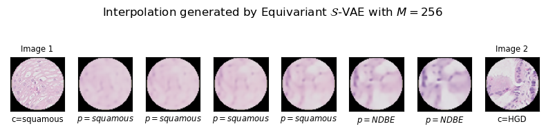
(a)

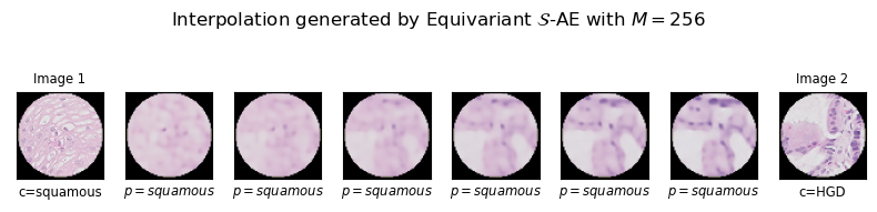
(b)

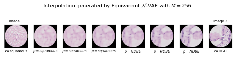
(c)

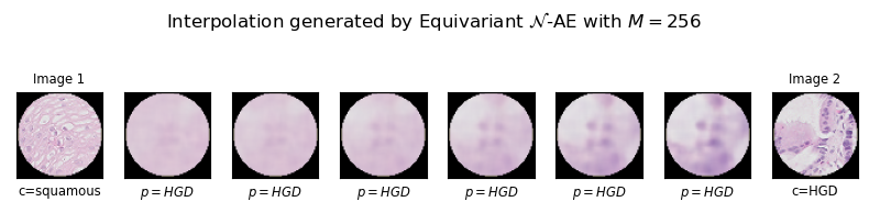
(d)

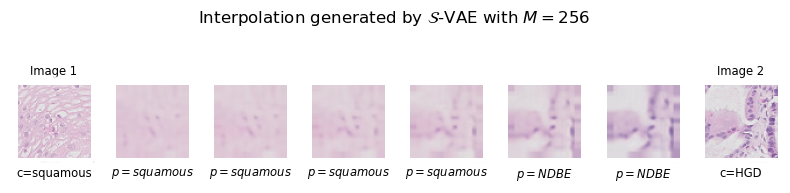
(e)

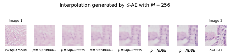
(a)

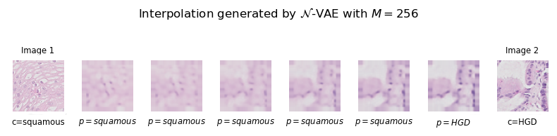
(b)

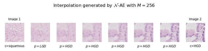
(c)

Figure B.19: Comparison of interpolations between the same image patches, generated by all different models and trained with latent dim of 256.

Bibliography

- Arvanitidis et al. (2017) Georgios Arvanitidis, Lars Kai Hansen, and Søren Hauberg. 2017. Latent space oddity: on the curvature of deep generative models. arXiv preprint arXiv:1710.11379.
- Bachmann et al. (2020) Gregor Bachmann, Gary Bécigneul, and Octavian Ganea. 2020. Constant curvature graph convolutional networks. In International Conference on Machine Learning, pages 486–496. PMLR.
- Batmanghelich et al. (2016) Kayhan Batmanghelich, Ardavan Saeedi, Karthik Narasimhan, and Sam Gershman. 2016. Nonparametric spherical topic modeling with word embeddings. In Proceedings of the conference. Association for computational linguistics. Meeting, volume 2016, page 537. NIH Public Access.
- Beik-Mohammadi et al. (2021) Hadi Beik-Mohammadi, Søren Hauberg, Georgios Arvanitidis, Gerhard Neumann, and Leonel Rozo. 2021. Learning riemannian manifolds for geodesic motion skills. arXiv preprint arXiv:2106.04315.
- Bengio et al. (2012) Yoshua Bengio, Aaron Courville, and Pascal Vincent. 2012. Representation learning: A review and new perspectives. arxiv e-prints, art. arXiv preprint arXiv:1206.5538.
- Bishop and Nasrabadi (2006) Christopher M Bishop and Nasser M Nasrabadi. 2006. Pattern recognition and machine learning. volume 4, chapter Continuous Latent Variables. Springer.
- Bronstein et al. (2017) Michael M Bronstein, Joan Bruna, Yann LeCun, Arthur Szlam, and Pierre Vandergheynst. 2017. Geometric deep learning: going beyond euclidean data. IEEE Signal Processing Magazine, 34(4):18–42.
- Cayton (2005) Lawrence Cayton. 2005. Algorithms for manifold learning. Univ. of California at San Diego Tech. Rep, 12(1-17):1.
- Chadebec et al. (2020) Clément Chadebec, Clément Mantoux, and Stéphanie Allassonnière. 2020. Geometry-aware hamiltonian variational auto-encoder.
- Chadebec et al. (2021) Clément Chadebec, Elina Thibeau-Sutre, Ninon Burgos, and Stéphanie Allassonnière. 2021. Data augmentation in high dimensional low sample size setting using a geometry-based variational autoencoder.
- Chen et al. (2018) Nutan Chen, Alexej Klushyn, Richard Kurle, Xueyan Jiang, Justin Bayer, and Patrick Smagt. 2018. Metrics for deep generative models. In International Conference on Artificial Intelligence and Statistics, pages 1540–1550. PMLR.
- Cohen and Welling (2016a) Taco Cohen and Max Welling. 2016a. Group equivariant convolutional networks. In International conference on machine learning, pages 2990–2999. PMLR.
- Cohen and Welling (2016b) Taco S Cohen and Max Welling. 2016b. Steerable cnns. arXiv preprint arXiv:1612.08498.
- Coifman et al. (2005) Ronald R Coifman, Stephane Lafon, Ann B Lee, Mauro Maggioni, Boaz Nadler, Frederick Warner, and Steven W Zucker. 2005. Geometric diffusions as a tool for harmonic analysis and structure definition of data: Diffusion maps. Proceedings of the national academy of sciences, 102(21):7426–7431.
- Cox and Cox (2008) Michael AA Cox and Trevor F Cox. 2008. Multidimensional scaling. In Handbook of data visualization, pages 315–347. Springer.
- Davidson et al. (2018) Tim R Davidson, Luca Falorsi, Nicola De Cao, Thomas Kipf, and Jakub M Tomczak. 2018. Hyperspherical variational auto-encoders. arXiv preprint arXiv:1804.00891.
- Davidson et al. (2019) Tim R. Davidson, Jakub M. Tomczak, and Efstratios Gavves. 2019. Increasing expressivity of a hyperspherical vae.
- Deng (2012) Li Deng. 2012. The mnist database of handwritten digit images for machine learning research. IEEE Signal Processing Magazine, 29(6):141–142.
- Detlefsen et al. (2022) Nicki Skafte Detlefsen, Søren Hauberg, and Wouter Boomsma. 2022. Learning meaningful representations of protein sequences. Nature communications, 13(1):1–12.
- Devlin et al. (2018) Jacob Devlin, Ming-Wei Chang, Kenton Lee, and Kristina Toutanova. 2018. Bert: Pre-training of deep bidirectional transformers for language understanding. arXiv preprint arXiv:1810.04805.
- Duque et al. (2020) Andrés F Duque, Sacha Morin, Guy Wolf, and Kevin Moon. 2020. Extendable and invertible manifold learning with geometry regularized autoencoders. In 2020 IEEE International Conference on Big Data (Big Data), pages 5027–5036. IEEE.
- Falorsi et al. (2018) Luca Falorsi, Pim De Haan, Tim R Davidson, Nicola De Cao, Maurice Weiler, Patrick Forré, and Taco S Cohen. 2018. Explorations in homeomorphic variational auto-encoding. arXiv preprint arXiv:1807.04689.
- Fan et al. (2022) Xiaomeng Fan, Yuwei Wu, Zhi Gao, Yunde Jia, and Mehrtash Harandi. 2022. Efficient riemannian meta-optimization by implicit differentiation. In Proceedings of the AAAI Conference on Artificial Intelligence, volume 36, pages 3733–3740.
- Fefferman et al. (2016) Charles Fefferman, Sanjoy Mitter, and Hariharan Narayanan. 2016. Testing the manifold hypothesis. Journal of the American Mathematical Society, 29(4):983–1049.
- Gruffaz et al. (2021) Samuel Gruffaz, Pierre-Emmanuel Poulet, Etienne Maheux, Bruno Jedynak, and Stanley Durrleman. 2021. Learning riemannian metric for disease progression modeling. Advances in Neural Information Processing Systems, 34:23780–23792.
- Gu et al. (2018) Albert Gu, Frederic Sala, Beliz Gunel, and Christopher Ré. 2018. Learning mixed-curvature representations in product spaces. In International Conference on Learning Representations.
- Hauberg (2018) Søren Hauberg. 2018. Only bayes should learn a manifold (on the estimation of differential geometric structure from data). arXiv preprint arXiv:1806.04994.
- He et al. (2020) Haiqi He, Nanzheng Chen, Yue Hou, Zhe Wang, Yong Zhang, Guangjian Zhang, and Junke Fu. 2020. Trends in the incidence and survival of patients with esophageal cancer: A seer database analysis. Thoracic Cancer, 11(5):1121–1128.
- Herstein (1991) Israel N Herstein. 1991. Topics in algebra. John Wiley & Sons.
- Hong et al. (2017) Jisu Hong, Bo-yong Park, and Hyunjin Park. 2017. Convolutional neural network classifier for distinguishing barrett’s esophagus and neoplasia endomicroscopy images. In 2017 39th Annual International Conference of the IEEE Engineering in Medicine and Biology Society (EMBC), pages 2892–2895.
- Hussein et al. (2022) Mohamed Hussein, Juana González-Bueno Puyal, David Lines, Vinay Sehgal, Daniel Toth, Omer F. Ahmad, Rawen Kader, Martin Everson, Gideon Lipman, Jacobo Ortiz Fernandez-Sordo, Krish Ragunath, Jose Miguel Esteban, Raf Bisschops, Matthew Banks, Michael Haefner, Peter Mountney, Danail Stoyanov, Laurence B. Lovat, and Rehan Haidry. 2022. A new artificial intelligence system successfully detects and localises early neoplasia in barrett’s esophagus by using convolutional neural networks. United European Gastroenterology Journal, 10(6):528–537.
- Jeong et al. (2021) Seungwoo Jeong, Wonjun Ko, Ahmad Wisnu Mulyadi, and Heung-Il Suk. 2021. Efficient continuous manifold learning for time series modeling. arXiv preprint arXiv:2112.03379.
- Kingma and Welling (2013) Diederik P Kingma and Max Welling. 2013. Auto-encoding variational bayes. arXiv preprint arXiv:1312.6114.
- Kourou et al. (2015) Konstantina Kourou, Themis P. Exarchos, Konstantinos P. Exarchos, Michalis V. Karamouzis, and Dimitrios I. Fotiadis. 2015. Machine learning applications in cancer prognosis and prediction. Computational and Structural Biotechnology Journal, 13:8–17.
- Kovenko and Bogach (2020) Volodymyr Kovenko and Ilona Bogach. 2020. A comprehensive study of autoencoders’ applications related to images. In IT&I Workshops.
- Krioukov et al. (2010) Dmitri Krioukov, Fragkiskos Papadopoulos, Maksim Kitsak, Amin Vahdat, and Marián Boguná. 2010. Hyperbolic geometry of complex networks. Physical Review E, 82(3):036106.
- Lafarge et al. (2020) Maxime W Lafarge, Josien PW Pluim, and Mitko Veta. 2020. Orientation-disentangled unsupervised representation learning for computational pathology. arXiv preprint arXiv:2008.11673.
- Li et al. (2022) Xintong Li, Chen Li, Md Mamunur Rahaman, Hongzan Sun, Xiaoqi Li, Jian Wu, Yudong Yao, and Marcin Grzegorzek. 2022. A comprehensive review of computer-aided whole-slide image analysis: from datasets to feature extraction, segmentation, classification and detection approaches. Artificial Intelligence Review, pages 1–70.
- Liu et al. (2022) Zhuang Liu, Hanzi Mao, Chao-Yuan Wu, Christoph Feichtenhofer, Trevor Darrell, and Saining Xie. 2022. A convnet for the 2020s. In Proceedings of the IEEE/CVF Conference on Computer Vision and Pattern Recognition, pages 11976–11986.
- Louis et al. (2019) Maxime Louis, Raphaël Couronné, Igor Koval, Benjamin Charlier, and Stanley Durrleman. 2019. Riemannian geometry learning for disease progression modelling. In Information Processing in Medical Imaging: 26th International Conference, IPMI 2019, Hong Kong, China, June 2–7, 2019, Proceedings 26, pages 542–553. Springer.
- Mikolov et al. (2013) Tomas Mikolov, Kai Chen, Greg Corrado, and Jeffrey Dean. 2013. Efficient estimation of word representations in vector space. arXiv preprint arXiv:1301.3781.
- Naesseth et al. (2017) Christian Naesseth, Francisco Ruiz, Scott Linderman, and David Blei. 2017. Reparameterization gradients through acceptance-rejection sampling algorithms. In Artificial Intelligence and Statistics, pages 489–498. PMLR.
- Nagano et al. (2019) Yoshihiro Nagano, Shoichiro Yamaguchi, Yasuhiro Fujita, and Masanori Koyama. 2019. A differentiable gaussian-like distribution on hyperbolic space for gradient-based learning.
- Ong et al. (2010) Chin-Ann J Ong, Pierre Lao-Sirieix, and Rebecca C Fitzgerald. 2010. Biomarkers in barrett’s esophagus and esophageal adenocarcinoma: predictors of progression and prognosis. World journal of gastroenterology: WJG, 16(45):5669.
- Piella (2014) Gemma Piella. 2014. Diffusion maps for multimodal registration. Sensors, 14(6):10562–10577.
- Radford et al. (2018) Alec Radford, Karthik Narasimhan, Tim Salimans, Ilya Sutskever, et al. 2018. Improving language understanding by generative pre-training.
- Rezende et al. (2014) Danilo Jimenez Rezende, Shakir Mohamed, and Daan Wierstra. 2014. Stochastic backpropagation and approximate inference in deep generative models. In International conference on machine learning, pages 1278–1286. PMLR.
- Riemann (1868) Bernhard Riemann. 1868. On the hypotheses which lie at the bases of geometry. Birkhäuser.
- Roweis and Saul (2000) Sam T Roweis and Lawrence K Saul. 2000. Nonlinear dimensionality reduction by locally linear embedding. science, 290(5500):2323–2326.
- Rumelhart et al. (1986) David E Rumelhart, Geoffrey E Hinton, and Ronald J Williams. 1986. Learning representations by back-propagating errors. nature, 323(6088):533–536.
- Shao et al. (2018) Hang Shao, Abhishek Kumar, and P Thomas Fletcher. 2018. The riemannian geometry of deep generative models. In Proceedings of the IEEE Conference on Computer Vision and Pattern Recognition Workshops, pages 315–323.
- Skopek et al. (2019) Ondrej Skopek, Octavian-Eugen Ganea, and Gary Bécigneul. 2019. Mixed-curvature variational autoencoders. arXiv preprint arXiv:1911.08411.
- Souvenir and Pless (2005) Richard Souvenir and Robert Pless. 2005. Isomap and nonparametric models of image deformation. In 2005 Seventh IEEE Workshops on Applications of Computer Vision (WACV/MOTION’05)-Volume 1, volume 2, pages 195–200. IEEE.
- de Souza Jr et al. (2018) Luis A de Souza Jr, Christoph Palm, Robert Mendel, Christian Hook, Alanna Ebigbo, Andreas Probst, Helmut Messmann, Silke Weber, and Joao P Papa. 2018. A survey on barrett’s esophagus analysis using machine learning. Computers in biology and medicine, 96:203–213.
- Tenenbaum (1997) Joshua Tenenbaum. 1997. Mapping a manifold of perceptual observations. Advances in neural information processing systems, 10.
- Tenenbaum et al. (2000) Joshua B Tenenbaum, Vin de Silva, and John C Langford. 2000. A global geometric framework for nonlinear dimensionality reduction. science, 290(5500):2319–2323.
- Thambawita et al. (2021) Vajira Thambawita, Inga Strümke, Steven A Hicks, Pål Halvorsen, Sravanthi Parasa, and Michael A Riegler. 2021. Impact of image resolution on deep learning performance in endoscopy image classification: An experimental study using a large dataset of endoscopic images. Diagnostics, 11(12):2183.
- Thomas (2022) Simon Myles Thomas. 2022. Representation learning for non-melanoma skin cancer using a latent autoencoder. arXiv preprint arXiv:2209.01779.
- Tifrea et al. (2018) Alexandru Tifrea, Gary Bécigneul, and Octavian-Eugen Ganea. 2018. Poincar’e glove: Hyperbolic word embeddings. arXiv preprint arXiv:1810.06546.
- Tosi et al. (2014) Alessandra Tosi, Søren Hauberg, Alfredo Vellido, and Neil D Lawrence. 2014. Metrics for probabilistic geometries. arXiv preprint arXiv:1411.7432.
- Ulrich (1984) Gary Ulrich. 1984. Computer generation of distributions on the m-sphere. Journal of the Royal Statistical Society: Series C (Applied Statistics), 33(2):158–163.
- Vadgama et al. (2022) Sharvaree Vadgama, Jakub Mikolaj Tomczak, and Erik J Bekkers. 2022. Kendall shape-vae: Learning shapes in a generative framework. In NeurIPS 2022 Workshop on Symmetry and Geometry in Neural Representations.
- Van Der Maaten et al. (2009) Laurens Van Der Maaten, Eric Postma, Jaap Van den Herik, et al. 2009. Dimensionality reduction: a comparative. J Mach Learn Res, 10(66-71):13.
- Wang and Wang (2019) Zhenxing Wang and Yadong Wang. 2019. Extracting a biologically latent space of lung cancer epigenetics with variational autoencoders. BMC bioinformatics, 20(18):1–7.
- Weiler and Cesa (2019) Maurice Weiler and Gabriele Cesa. 2019. General e (2)-equivariant steerable cnns. Advances in Neural Information Processing Systems, 32.
- Van der Wel et al. (2016) M. Van der Wel, Marnix Jansen, Michael Vieth, and Sybren Meijer. 2016. What makes an expert barrett’s histopathologist? volume 908, pages 137–159.
- van der Wel et al. (2020) Myrtle J van der Wel, Helen G Coleman, Jacques JGHM Bergman, Marnix Jansen, and Sybren L Meijer. 2020. Histopathologist features predictive of diagnostic concordance at expert level among a large international sample of pathologists diagnosing barrett’s dysplasia using digital pathology. Gut, 69(5):811–822.
- Wold et al. (1987) Svante Wold, Kim Esbensen, and Paul Geladi. 1987. Principal component analysis. Chemometrics and intelligent laboratory systems, 2(1-3):37–52.
- Xu and Durrett (2018) Jiacheng Xu and Greg Durrett. 2018. Spherical latent spaces for stable variational autoencoders. arXiv preprint arXiv:1808.10805.
- Yang et al. (2018) Tao Yang, Georgios Arvanitidis, Dongmei Fu, Xiaogang Li, and Søren Hauberg. 2018. Geodesic clustering in deep generative models. arXiv preprint arXiv:1809.04747.
- Zeune et al. (2020) Leonie L Zeune, Yoeri E Boink, Guus van Dalum, Afroditi Nanou, Sanne de Wit, Kiki C Andree, Joost F Swennenhuis, Stephan A van Gils, Leon WMM Terstappen, and Christoph Brune. 2020. Deep learning of circulating tumour cells. Nature Machine Intelligence, 2(2):124–133.