Universality of the superfluid Kelvin-Helmholtz instability by single-vortex tracking

Abstract

At the interface between two fluid layers in relative motion, infinitesimal fluctuations can be exponentially amplified, inducing vorticity and the breakdown of the laminar flow. This process, known as the Kelvin-Helmholtz instability ^{1, 2}, is responsible for many familiar phenomena observed in the atmosphere ^{3, 4}, and the oceans ^{5, 6}, as well as in astrophysics ⁷, and it is one of the paradigmatic routes to turbulence in fluid mechanics ^{8, 9, 10, 11}. While in classical hydrodynamics the instability is ruled by universal scaling laws, to what extent universality emerges in quantum fluids is yet to be fully understood. Here, we shed light on this matter by triggering the Kelvin-Helmholtz instability in atomic superfluids across widely different regimes, ranging from weakly-interacting bosonic to strongly-correlated fermionic pair condensates. Upon engineering two counter-rotating flows with tunable relative velocity, we observe how their contact interface develops into an ordered circular array of quantized vortices, which loses stability and rolls up into clusters in close analogy with classical Kelvin-Helmholtz dynamics ¹². We extract the instability growth rates by tracking the position of individual vortices and find that they follow universal scaling relations, predicted by both classical hydrodynamics ^{13, 14} and a microscopic point-vortex model ^{15, 16}. Our results connect quantum and classical fluids revealing how the motion of quantized vortices mirrors the interface dynamics and open the way for exploring a wealth of out-of-equilibrium phenomena, from vortex-matter phase transitions ^{17, 18} to the spontaneous emergence of two-dimensional quantum turbulence ^{19, 20, 21}.

A close relationship exists between vortices and shear-flow instabilities in fluid mechanics. In classical hydrodynamics, the interface between two fluid layers in relative motion is identified by an ideal surface containing an infinite number of line vortices, namely a vortex sheet ¹⁴. More than one century ago, Lord Kelvin and von Helmholtz predicted the dynamical instability of such a vortex sheet ^{1, 2}. The Kelvin-Helmholtz instability (KHI) initially manifests itself as a wave-like deformation of the interface, exponentially growing in time with a rate proportional to the relative velocity between the two fluids (Fig. 1a). It quickly leads to the twisting of the vortex sheet ^{13, 14} and eventually to a turbulent mixing of spiraling structures ¹¹. Starting from the seminal experiments by Reynolds in 1883 ²², the KHI has been the subject of extensive research and experimentation ^{23, 24, 25, 26, 27}.

The last few decades have seen exciting advances in the field of superfluidity ²⁸ – in particular in ultracold atomic systems ²⁹ – owing to our ever-increasing capability to manipulate pristine quantum systems in which vorticity is quantized, and dissipation occurs through different channels from those in ordinary fluids. A natural question is whether these key differences affect the onset and the microscopic nature of flow instabilities and whether the universal KHI scaling relations established in classical hydrodynamics is sufficiently general to include superfluids, particularly in the presence of strong interactions. Theoretical investigations have so far been focused mostly on the stability of the interface between distinct sliding fluid components, such as superfluid or normal phases of the same liquid ^{30, 31} or immiscible components in binary Bose-Einstein condensates ^{32, 33, 34} (BECs). Experimental observations remain limited to the interface between the A and B phases of ³He in a rotating cryostat ^{35, 36}. All these systems involve phases with distinct physical properties, which complicate the picture due to the presence of additional Rayleigh-Taylor²⁰ and counter-superflow instabilities³³.

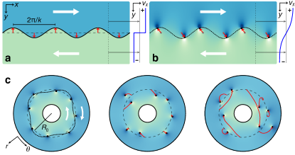
Figure 1: Kelvin-Helmholtz instability in classical and quantum fluids. a, The interface (horizontal dashed line) separating two counter-propagating classical flows undergoes KHI, developing a wave-like deformation with a characteristic wavenumber $k$. b, In single-component superfluids, the interface modes are replaced by the collective excitations of a one-dimensional vortex lattice. The dotted sinusoidal line illustrates one of these modes, with the vortices displaced with respect to their initial positions, as indicated by the red arrows. In both a and b panels, we display on the right vertical cuts of the velocity profiles along the transverse direction. c, Left panel: in counter-rotating flows, the KHI arises as a deformation of a circular vortex necklace. The circle of radius $R_{0}$ (dashed line) interpolates the initial vortex positions. The winding number $m$ of the deformation is related to the azimuthal wavenumber $k$ via $m=kR_{0}$. As an example, the mode $m=4$ is displayed (sinusoidal dotted curve). The central and right panels display the later stages of vortex pairing and irregular mixing, together with the corresponding vortex trajectories (red curved arrows). In all panels, the background colors indicate the magnitude of the velocity component tangential to the shear layer, with the flow directions specified by white arrows.

We follow a conceptually simpler, minimal approach to the KHI by creating a shear flow in a single-component superfluid ^{37, 38}. In such a system, the continuous vortex sheet at the layer between the two flows is replaced by an array of quantized vortices^{37, 39} (Fig. 1b). The tangential flow varies smoothly everywhere except at the position of the vortex cores, resulting in a finite-thickness layer, i.e. an effective interface. In a ring-shaped geometry with two counter-rotating flows, the classical circular vortex sheet transforms into a circular array of quantized vortices, or a vortex necklace, with radius $R_{0}$. While this geometry is equivalent to the planar case for what concerns the instability mechanism, it has the advantage of genuinely imposing periodic boundary conditions, preventing possible fluid accumulation at the system boundaries. By imaging the individual vortex motion, we show that the vortex necklace is unstable: infinitesimal fluctuations in the system rapidly break the periodicity and trigger complex dynamics, with nearby vortices rolling up and eventually displaying an irregular, albeit deterministic, motion (Fig. 1c). We experimentally demonstrate that this behaviour corresponds to a discrete version of Kelvin-Helmholtz dynamics, where collective excitations of the vortex lattice exhibit universal KHI scalings across different superfluid regimes. Our observations establish homogeneous superfluid rings of ultracold fermions as a versatile laboratory for quantum fluid-dynamics experiments. We overcome typical difficulties that complicate experiments with helium quantum fluids ^{35, 36}, especially in terms of precise initial flow control, suppression of the normal fraction, and single-vortex detection.

Our experiment starts with two thin and uniform Fermi superfluids comprising $N_{p}\simeq 3\times 10^{4}$ pairs of fermionic ⁶Li atoms (see Methods). Interactions between atoms forming the pairs are encoded in the $s$-wave scattering length $a$. This can be tuned through a broad Feshbach resonance, entering different superfluid regimes ranging from weakly interacting BECs of tightly bound molecules ($1/k_{F}a>1$) to strongly correlated unitary Fermi gases (UFG, $1/k_{F}a\simeq 0$) and Bardeen-Cooper-Schrieffer (BCS, $1/k_{F}a<0$) superfluids. Here, $k_{F}=(ME_{F}/\hbar^{2})^{1/2}$ is the Fermi wavevector, estimated from the system global Fermi energy $E_{F}$, and $M$ is the mass of a fermion pair. The superfluids are confined into concentric annular optical traps initially separated by a narrow potential barrier, resulting in two reservoirs with equal density $n_{2D}=$4.96(2)\text{\,}\mu\mathrm{m}^{-2}$$ (see Fig. 2a). Sample temperatures are well below the critical temperature $T_{c}$ of the superfluid transition, $T=0.3(1)\,T_{c}$, corresponding to near-unity superfluid fractions in all interaction regimes. The superfluid healing length $\xi$ is always smaller than the vertical cloud size, making the superfluid dynamics three-dimensional. In contrast, vortex dynamics remain two-dimensional since only a few Kelvin modes of vortex lines are expected to be thermally and geometrically accessible at our temperature ⁴⁰.

We excite persistent flows in each reservoir by optically imprinting a dynamical phase onto the superfluid rings ⁴¹. In particular, we drive independent currents by shining oppositely oriented, azimuthal light gradients onto the internal and external rings (see Methods). With this procedure, we set integer quantized circulations $w_{i,e}$ with corresponding velocity fields $v_{i,e}(r)=\hbar w_{i,e}/(Mr)$, where $r$ is the distance from the ring center, and the indices $i,e$ refer to the internal and external rings, respectively. The relative velocity at the interface equals $\Delta v=\hbar(w_{e}-w_{i})/(MR_{0})$, where $R_{0}$ is the radius of the circular potential barrier separating the reservoirs. In all interaction regimes, we fix $w_{e}=-w_{i}$ and only consider velocities $\Delta v_{\mathrm{max}}<0.7\,c_{s}$, where $c_{s}$ is the measured speed of sound in bulk ⁴⁰.

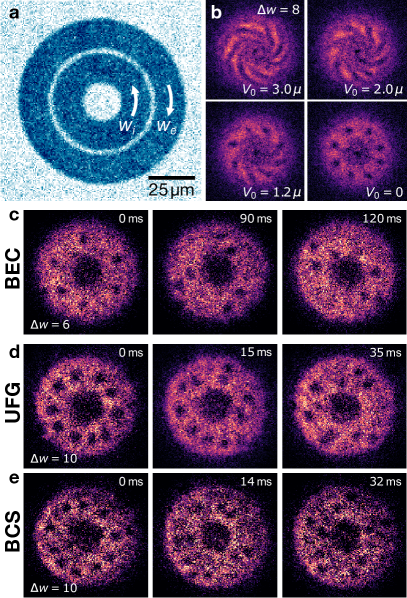
Figure 2: Flow preparation and Kelvin-Helmholtz dynamics. a, In situ density profile of two concentric counter-rotating superfluids (BEC), set in relative motion by a phase-imprinting technique while being separated by a potential barrier with FWHM $=$1.4(1)\text{\,}\mu\mathrm{m}$$. b, Single-shot TOF images in the BEC regime for $\Delta w=8$, as the barrier height $V_{0}$ is gradually lowered from $V_{0}\approx 3.5\,\mu$ to 0, where $\mu$ is the superfluid chemical potential (Methods). c–e, Typical single-shot TOF images of the vortex patterns obtained at different times $t\geq 0$ after merging the two superfluids in distinct interaction regimes: c. BEC at $1/k_{F}a=4.3(1)$ with $\Delta w=6$; d, UFG at $1/k_{F}a=0.0(1)$ with $\Delta w=10$; and e, BCS superfluid at $1/k_{F}a=-0.3(1)$ with $\Delta w=10$. In all interaction regimes, the vortex necklace destabilizes for $t>0$, and few-vortex clusters form.

We merge the two counter-rotating superfluids by gradually lowering the barrier potential. To follow the evolution of the flow, we image the atomic density profile after a short time-of-flight (TOF) expansion at varying times during the barrier removal. As shown in Fig. 2b, as long as the barrier separates the two superfluid rings, a spiral interference pattern is observed, due to the presence of an azimuthal phase gradient between the rings. The number of spiral arms matches the number $\Delta w\equiv|w_{e}-w_{i}|$ of $2\pi$ phase-slips at the circular interface ^{42, 41}. Eventually, when the barrier is completely removed and the two superfluids come into full contact ($t=0$), we observe a necklace of $N_{v}=\Delta w$ singly-charged, quantized vortices ^{38, 37} with the same circulation sign determined by vorticity³⁷. Soon after the vortex necklace emerges, its periodicity breaks down and vortices start pairing in a quasi-synchronous process. As time progresses, metastable clusters of increasingly larger size form, following trajectories reminiscent of the characteristic Kelvin-Helmholtz roll-up dynamics (Fig. 2c-e).

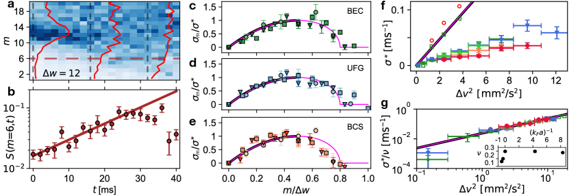
Figure 3: Analysis of Kelvin-Helmholtz instability across the BEC-BCS crossover. a, Normalized angular structure factor $s(m,t)$ for a UFG superfluid and $\Delta w=12$. Solid red lines represent vertical cuts $s(m)$, corresponding to angular spectra at different times, and the dashed horizontal line indicates the expected most unstable mode. b, Time evolution of $s$ for the most unstable mode, $m^{*}=6$. An exponential fit of the data (line) is used to extract the growth rate $\sigma^{*}$. Error bars denote the standard error of the mean over $\sim 20$ experimental realizations. c–e, Normalized dispersion relations, $\sigma_{m}/\sigma^{*}$, as a function of $m/\Delta w$ for: c, BEC [$1/k_{F}a=4.3(1)$]; d, UFG [$1/k_{F}a=0.0(1)$]; and e, BCS [$1/k_{F}a=-0.3(1)$] superfluids. Rates are shown for different $\Delta w=8,10,12$, respectively denoted by circles, squares, and triangles. Solid lines show the rates predicted by the PVM in Eq. (1) (black line) and by Rayleigh’s Eq. (2) using $\delta=0.8\hbar/M\Delta v$ (magenta line). f, Experimental and theoretical scaling of $\sigma^{*}$ against $\Delta v^{2}$ in different interaction regimes. Filled symbols corresponds to experimental data: BCS ($1/k_{F}a=-0.5(1)$, red diamonds), ($1/k_{F}a=-0.3(1)$, orange diamonds); UFG ($1/k_{F}a=0.0(1)$, blue triangles); and BEC ($1/k_{F}a=4.3(1)$, dark green stars), ($1/k_{F}a=8.3(3)$, light green circles). Open symbols refer to GP simulations at $T=0$ (open green squares) and cZNG simulations at $T/Tc=0.4$ (open red circles) for $1/k_{F}a=4.3(1)$. Solid lines refer to Rayleigh’s (magenta) and PVM (black) predictions. g, Experimental growth rates rescaled by the interaction-dependent constant $\nu$, shown in the inset as a function of $1/k_{F}a$. In panels, c–g, vertical error bars denote fitting $1\sigma$-errors, while horizontal ones reflect the experimental uncertainty on the initial vortex number.

The stability of the vortex necklace can be analyzed using the point vortex model⁴⁰ (PVM), where each vortex is treated as a point particle advected by the velocity field generated by all other vortices. The vortex motion is thus determined by the background flow which, in turn, emerges as a phenomenon associated with the vortex dynamics. The KHI appears as a departure from the initial ordered vortex configuration with characteristic rates given by ^{15, 16}

$$\sigma_{\mathrm{PVM}}(k,\Delta v)=\frac{\Gamma k}{2d_{v}}\left(1-\frac{kd_{v}}{2\pi}\right),$$ (1)

where $k$ is the perturbation mode wavenumber, $\Gamma=h/M$ is the quantized vortex circulation, and $d_{v}=h/(M\Delta v)$ is the initial inter-vortex separation. The maximum growth rate $\sigma^{*}$, i.e. the growth rate of the most unstable mode, is reached for $k^{*}=\pi/d_{v}$. This particular wavenumber sets a fundamental scaling law, $\sigma^{*}\propto{\Delta v}^{2}$, providing a direct hallmark of the instability. The mode $k^{*}$ is also the largest wavenumber that can be supported in a one-dimensional array of lattice constant $d_{v}$ (i.e. a mode with a wavelength equal to $2d_{v}$). As such, the model can be meaningfully applied to describe our data only for $k\leq k^{*}$. In the limit of closely packed vortices $d_{v}\rightarrow 0$, Eq. (1) reduces to $\sigma_{\mathrm{PVM}}\sim\frac{1}{2}k\Delta v$, which equals Kelvin’s growth rate of a continuous vortex sheet¹⁴ (i.e., a zero-width interface). The PVM thus extends the traditional KHI result to the case of a discrete vortex sheet formed by a finite number of vortices, providing thus a microscopic description of the instability. It predicts also a smooth change of the tangential flow between the two layers, except at the position of the vortices, resulting in a finite-size effective interface with half-width $\delta=\hbar/(M\Delta v)$ (Fig. 1b, and Ref. 40).

In classical fluid mechanics, the problem of the stability of a finite-width shear layer was first analyzed by Rayleigh ⁴³ who derived an interface-dependent growth rate as:

$$\sigma_{\mathrm{R}}(k,\Delta v)=\mathrm{Im}\frac{\Delta v}{4\delta}\sqrt{(2k\delta-1)^{2}-e^{-4k\delta}}.$$ (2)

Here, $\delta$ is the interface width and depends on the fluid’s specifics and on the flow shear velocity. According to Eq. (2), the instability only occurs for $k\delta\leq 0.64$, while the system is stable against perturbations with higher wavenumbers ¹⁴.

In the experiment, we reconstruct the evolution of the vortex necklace by tracking vortex positions over time and characterizing it through the vortex structure factor $S$. This provides a quantitative description of the lattice structure, and its deformation from the initial periodic configuration ⁴⁴. In our circular geometry, although vortices move both in radial and azimuthal directions, the vortex crystal modes are purely azimuthal (see dotted line in Fig. 1c). Therefore, to decompose the motion, it is natural to introduce the angular structure factor (see Methods), defined as $S(m,t)=(1/N_{v})\sum_{j,l}\exp[im(\theta_{j}(t)-\theta_{l}(t)]$. Here, $\theta_{j}(t)$ is the angular position of the $j$-th vortex, and $m$ is the integer winding number of the mode, defined as $m=kR_{0}$. Figure 3a displays $s(m,t)=S(m,t)/N_{v}$ measured for $1/k_{F}a=0.0(1)$ and $\Delta w=12$. The spectral peak at $m=\Delta w$, characteristic of a periodic necklace, evolves towards lower angular modes while it simultaneously broadens (see angular spectra plotted in red color). Similar behaviour is found in all interaction regimes. This indicates the breakdown of the necklace structure while an increasing number of modes become populated. We extract the instability rate of each mode $m$ by analyzing the initial time evolution of $s(m,t)$. For most modes, we observe that $s(m,t)$ grows exponentially in time as $s(m,t)\sim e^{2\sigma_{m}t}$, where $\sigma_{m}$ is the growth rate of the $m$-th mode, signaling the onset of a linearly unstable flow ^{40, 14}. As an example, in Fig. 3b we present the behavior for $m=6$.

In Fig. 3c-e, we show the normalized dispersion relations $\sigma_{m}/\sigma^{*}$ as a function of $m/\Delta w$ for BEC, UFG, and BCS superfluids. All the measured rates are in good agreement with the expected trends from the PVM [Eq. (1)] and Rayleigh [Eq. (2)] formulas using $\delta=0.8\hbar/(M\Delta v)$ (see Ref. 40 for the determination of $\delta$). We see that the instability occurs for $m\lesssim 0.8\,\Delta w$ matching the value predicted by the Rayleigh formula. The most unstable mode is found at $m^{*}\sim 0.5\,\Delta w$, as analytically derived from Eq. (1) and confirmed by Eq. (2) using the above value for $\delta$. In Fig. 3f, the extracted $\sigma^{*}$ for different superfluid regimes is plotted as a function of the relative velocity. The measured growth rates display a power law increase, $\sigma^{*}\propto{\Delta v}^{\alpha}$, with fitted exponent $\alpha=1.98(3)$ in agreement with the expected $\alpha=2$ within the experimental uncertainty ⁴⁰. Upon rescaling the fitted slopes with an interaction-dependent factor $\nu$ (see Fig. 3g), all data collapse on a single line over more than one decade. These scaling properties together with the normalized dispersion relations in Fig. 3c-e provide clear evidence of KHI dynamics in superfluids and of its universality across the BEC-BCS crossover.

The data in Fig. 3f are compared with Eqs. (1) and (2), and with 3D numerical simulations based on Gross-Pitaevskii (GP) equation and collisionless Zaremba-Nikuni-Griffin (cZNG) model^{11, 14}. While theoretical rates – analytical and numerical – agree quantitatively with each other, the measured ones show systematically lower values. In classical fluids, dissipation effects (e.g. surface tension, viscosity) typically tend to stabilize the system, leading to smaller growth rates ^{14, 13}. In our system, temperature effects and technical imperfections such as spurious vortices and other density excitations originated from the barrier removal, as well as from a non-ideal imprinting procedure, ^{41, 40} are possible sources of dissipation. These effects are encapsulated phenomenologically in the $\nu$ parameter shown in the inset of Fig. 3g. For $1/k_{F}a\geq 0$, $\nu$ show a nearly constant value of $0.29(1)$, while BCS superfluids with $1/k_{F}a<0$ display a stronger deviation from the ideal case ($\nu=1$). The numerical simulations of the cZNG model in the BEC limit suggest no significant role of the small thermal fraction. On the other hand, in the BCS regime, we expect the combined effects of the thermal component and Andreev vortex-bound states to enter into play, opening a further dissipative channel ^{47, 48}. A quantitative understanding of the microscopic mechanisms connecting non-local vortex dynamics to dissipation, especially in presence of strong correlations, remains an open problem ^{49, 50}.

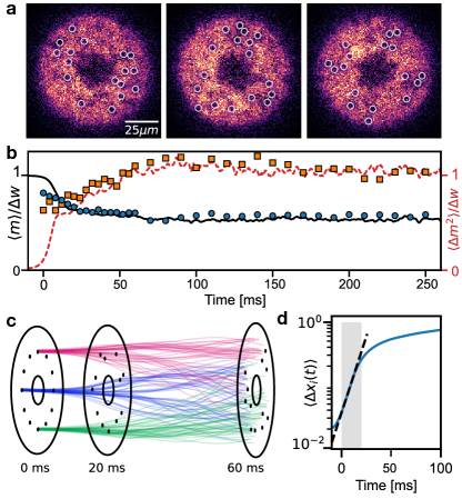
Figure 4: Nonlinear vortex dynamics. a, Single-shot TOF images of vortex patterns acquired after $36$ ms of evolution, showing $2-$, $3-$, and $4-$fold vortex cluster symmetries. Images are acquired for a BEC superfluid starting from nominally identical necklaces with $N=16$. b, Time evolution of the mean winding number $\langle m\rangle$ (circles) and its variance $\langle\Delta m^{2}\rangle$ (squares) normalized to $\Delta w$ for $1/k_{F}a=4.3(1)$ and $\Delta w=12$, averaged over $\sim\,$20 experimental realizations. The data are compared with PVM simulations (black-solid and red-dashed lines). c, Trajectories of three vortices (colored lines) belonging to nearly-identical necklaces with $N=12$. A set of 40 initial vortex positions are picked randomly, each within a range of one healing length $\xi\approx 0.5\mu$m around their reference value, for which the necklace is perfectly periodic. We show the vortex pattern at $t=0,20,60$ms for one realization. d, Mean-distance between each-vortex trajectory calculated as a function of time by averaging over $40$ nearly-identical random initial conditions, as described above, and over $N_{v}=12$ vortices. The distances are normalized to the mean separation of any given two points in the ring geometry (Methods). At short times, $t<20$ ms (shaded area), the separation between trajectories grows exponentially (dashed line) with a characteristic maximal Lyapunov exponent of $\Lambda=0.111(5)\,\text{ms}^{-1}$, in agreement with the maximum growth rate obtained for the KHI with $\Delta w=12$, $\sigma_{PVM}^{*}=0.127(5)\,\text{ms}^{-1}$.

After the initial stage of the instability, with characteristic time $1/\sigma^{*}$, the vortex dynamics enter a nonlinear regime with vortex clusters forming and fragmenting as time progresses while conserving the total vortex number. Starting from nominally identical initial conditions, vortices cluster in arrangements displaying different symmetries, as shown in Fig. 4a. Which of these symmetries appears at a given time hinges on the initial conditions and fluctuations in the system. Averaging over different realizations, we observe the system exploring widely different configurations, losing information about the initial order. In particular, the mean winding number $\langle m\rangle$ is nearly constant in time around $\Delta w/2$, while the variance $\langle\Delta m^{2}\rangle$ saturates to the vortex number $\Delta w$ (see Fig. 4b). This indicates that the system reaches a steady state, where all modes are significantly populated. PVM simulations starting with nearly identical configurations reproduce quantitatively the experimental data, suggesting that vortices tend to spread over the whole system volume (Fig. 4c).

This extreme sensitivity to the initial conditions, where arbitrarily small differences lead to exponential divergence of trajectories, is typically quantified by an average divergence rate known as the maximal Lyapunov exponent ⁵¹, $\Lambda$. We calculate $\Lambda$ by comparing the vortex trajectories of the different PVM simulations, computing their relative separation as a function of time (see Fig. 4c-d and Methods). Interestingly, we observe that the average separation between same-vortex trajectories grows exponentially, $\sim e^{\Lambda t}$, with a rate $\Lambda$ similar to the maximal KHI growth rate, $\sigma_{\mathrm{PVM}}^{*}$ (Fig. 4d). While $\sigma^{*}$ quantifies the collective motion of the necklace, $\Lambda$ refers to the trajectory of a single vortex. This connection clarifies the role of quantized vortices in defining the interface dynamics and the KHI as the mechanism behind the necklace breakdown. For $t\gg 1/\Lambda$, the distance between trajectories tends to saturate to the average separation of two random points in the system (set by the value $1$ in the graph). This is due to the finite-size effects that constrain the trajectories divergence, eventually leading to the attainment of boundary-dominated dynamical equilibrium. We remark that a positive maximal Lyapunov exponent implies the unpredictability of a deterministic system ⁵¹, and is generally associated with chaotic advection, and turbulent flows ⁵². Classically, the KHI drives the system into a turbulent state portrayed by an irregular – sensitive to initial conditions – mixing of spiraling structures at different scales ¹¹. The intertwined vortex trajectories shown in Fig. 4c are reminiscent of this scenario.

Our observation of the superfluid Kelvin-Helmholtz instability showcases a pristine example of an emergent phenomenon in which quantized vortices play the role of elementary constituents: the instability arises from the coherent motion of vortices, here acting simultaneously as sources and probes of the unstable flow. The same microscopic mechanism operates in all superfluid regimes, and it underlies the observed universal behaviour, which interestingly belongs to the class of classical inviscid fluids with finite-size shear layers. We anticipate our results to be of relevance for diverse non-equilibrium phenomena in strongly correlated quantum matter, ranging from rapidly rotating quantum gases ³⁹ to pulsar glitches ⁵³ and neutron star mergers ⁵⁴. Our findings also set the starting point to explore a variety of vortex matter phase-transitions in fermionic superfluids ⁵⁵, including negative temperature and non-trivial cluster states ^{56, 17, 18, 57}, even in presence of dissipative mechanisms resulting from vortex-vortex and vortex-quasiparticles interactions ^{58, 50}. An exciting direction for future experiments concerns the cascade of secondary instabilities towards the spontaneous onset of quantum turbulence ^{37, 20, 36}, exploring a route complementary to external forcing ^{59, 60} to probe its underlying microscopic mechanisms from the few- to the many-vortex perspective.

I Acknowledgements

We thank Iacopo Carusotto, Nigel Cooper, and Giovanni Modugno for valuable comments on the manuscript, and the Quantum Gases group at LENS for fruitful discussions. This work was supported by the European Research Council under Grant Agreement No. 307032, the Italian Ministry of University and Research under the PRIN2017 project CEnTraL, and European Union’s Horizon 2020 research and innovation program under the Qombs project FET Flagship on Quantum Technologies Grant Agreement No. 820419 and Marie Skłodowska-Curie Grant Agreement No. 843303, and the Research Fund (1.220137.01) of UNIST (Ulsan National Institute of Science and Technology). Acknowledge financial support from: PNRR MUR project PE0000023-NQSTI M.M. acknowledges support from Grant No. PID2021-126273NB-I00 funded by MCIN/AEI/10.13039/501100011033 and “ERDF - A way of making Europe”, and from the Basque Government through Grant No. IT1470-22.

II Methods

II.1 Sample preparation

We prepare fermionic superfluid samples by evaporating a balanced mixture of the two lowest hyperfine spin states $|F,m_{F}\rangle=|1/2,\pm 1/2\rangle$ of ⁶Li, near their scattering Feshbach resonance at $832\text{\,}\mathrm{G}$ in an elongated, elliptic optical dipole trap, formed by horizontally crossing two infrared beams at a $14^{\circ}$ angle. At the end of the evaporation, we sweep the magnetic field to the desired interaction regime. A repulsive $\mathrm{TEM_{01}}$-like optical potential at $532\text{\,}\mathrm{n}\mathrm{m}$ with a short waist of about $13\text{\,}\mu\mathrm{m}$ is then adiabatically ramped up before the end of the evaporation to provide strong vertical confinement, $\omega_{z}\simeq 2\pi\times 400$ Hz. Successively, a box-like potential is turned on to trap the resulting sample in a circular region of the $x$–$y$ plane. This circular box is tailored using a Digital Micromirror Device (DMD). When both potentials have reached their final configuration, the infrared lasers forming the crossed dipole trap are adiabatically extinguished, completing the transfer into the final uniform pancake trap⁴⁷. Finally, to create the pair of superfluid rings at rest we dynamically change the DMD-tailored potential. We first create the hole at the center of the initial disk and then dynamically increase its size until reaching a radius of $R_{i}=$10.0(2)\text{\,}\mu\mathrm{m}$$. Finally, an optical barrier separating the two superfluid rings is adiabatically raised at $R_{0}=$27.5(2)\text{\,}\mu\mathrm{m}$$. A residual radial harmonic potential of $2.5\text{\,}\mathrm{H}\mathrm{z}$ is present due to the combined effect of an anti-confinement provided by the $\mathrm{TEM_{01}}$ laser beam in the horizontal plane and the confining curvature of the magnetic field used to tune the Feshbach resonance. This weak confinement has a negligible effect on the sample over the $R_{e}=$45.0(2)\text{\,}\mu\mathrm{m}$$ radius of our box trap, resulting in an essentially homogeneous density.

II.2 Phase-imprinting procedure

We excite controllable persistent current states in each of the two rings by using the phase imprinting protocol described in Ref. 41. Using the DMD we create an optical gradient along the azimuthal direction, namely $U(r,\theta)=U_{0}\,\theta/2\pi\times\mathrm{sign}(r-R_{0})$. By projecting such a potential over a time $t_{I}<\hbar/\mu$, we imprint a phase $\phi(r,\theta)=U(r,\theta)\,t_{I}/h$ onto the superfluid wavefunction. By suitably tuning the imprinting time $t_{I}$ and the gradient intensity $U_{0}$, we excite well-defined winding number states in each of the two rings in a reproducible way. We measure the imprinted circulations using an interferometric probe: we let the two rings expand for $3$ ms of time of flight (TOF) and then image the resulting spiral-shaped interference pattern. The first panel of Fig. 2b shows such an interferogram for $\Delta w=8$. In particular, the number of spirals in the interferogram yields the relative winding number $\Delta w$ between the two rings ^{42, 41}. Additionally, we independently check that before the imprinting procedure, the inner ring is in the $w=0$ state by realizing a similar experimental protocol now in a geometry similar to the reported in Ref. 41. All circulation states excited in the two rings have been observed to persist for several hundreds of ms ⁴¹, except for $\Delta w>\mathrm{12}$ in the BCS regimes. Nevertheless, we observe these states to not decay for the typical timescale of the observed KHI $t<$40\text{\,}\mathrm{m}\mathrm{s}$$. To reduce the effect of extra density excitation in the system on the KHI dynamics, we wait $300\text{\,}\mathrm{m}\mathrm{s}$ after imprinting before removing the barrier between the superfluids.

II.3 Vortex imaging and tracking

We trigger the KHI dynamics by removing the circular barrier separating the two ring superfluids. In particular, we lower down its intensity by opportunely changing the DMD pattern. The barrier removal process takes 28 ms and brings the system into the vortex necklace configuration of Fig 2. We confirm that the duration of the barrier removal does not affect significantly the dynamics. Removing the barrier over time scales faster than 10 ms creates unwanted excitations such as solitonic structures. To image the vortices in the BEC regime, we acquire the TOF image of the superfluid density, where vortices appear as clear holes. In particular, we abruptly switch off the vertical confinement and at the same time, we start to ramp down the DMD potential, removing it completely in $1\text{\,}\mathrm{m}\mathrm{s}$. Then, we let the system evolve further for $2.2\text{\,}\mathrm{m}\mathrm{s}$ of TOF and then acquire the absorption image. This modified TOF method allows for to maximization of the vortex visibility. However, the small condensed fraction in the strongly-interacting regime makes it impossible to detect vortices with this simple method. Therefore, in the UFG and BCS regimes, we employ the technique developed in Ref. 47: we add a linear magnetic field ramp of $4-5$ ms to $700\text{\,}\mathrm{G}$ before the imaging to map the system in a BEC superfluid.

The position of the vortices is tracked manually in each acquired image. The error on the position of the vortex is limited by the size of the vortex after the TOF sequence. To estimate it we perform a Gaussian fit of the vortex density hole and obtain a waist of $\sim 1.0-$1.4\text{\,}\mu\mathrm{m}$$ for all interaction regimes.

II.4 Point Vortex Model (PVM)

We consider a two-dimensional fluid containing N point vortices with quantized circulations $\Gamma=h/M$. When the inter-vortex separation is greater than a few healing lengths, vortices are advected by the velocity field created by other vortices. The equation of motion of each vortex is $d\vec{r}_{i}/dt=\vec{v_{i}}^{0}$, where $\vec{v_{i}}^{0}$ is the velocity field created by all the other vortices. If we consider a 1D array of equispaced vortices at coordinates $(x_{n},y_{n})=(d_{v}/2+nd_{v},0)$, moving in a 2D space of coordinates $(x,y)$ without boundaries, the tangential velocity of the superfluid flow can be written as:

$$v_{x}(x,y)=-\frac{\Gamma}{2d_{v}}\frac{\sinh\left(2\pi y/d_{v}\right)}{\cosh\left(2\pi y/d_{v}\right)+\cos\left(2\pi x/d_{v}\right)}.$$

From this relation, the finite-size width of the effective interface is naturally expressed in units of $\delta=d_{v}/(2\pi)$, or equivalently $\delta=\hbar/(M\Delta v)$.

When considering the ring geometry, $\vec{v_{i}}^{0}$ must take into account the boundary conditions, namely that the flow must have a zero radial component at both the internal ($R_{i}$) and external ($R_{e}$) radii. We include the boundary conditions by using the method of image vortices ⁴⁰, and solve the equation of motions for the vortex necklace configuration in the ring with the Runge-Kutta method of fourth order. From the obtained trajectories of the vortices, $\vec{r}_{i}(t)$ we compute the normalized angular structure factor $s(m,t)$.

II.5 Angular structure factor analysis

At $t=0$, the one-dimensional angular structure factor of a finite array of $N$ vortices placed in a perfect necklace arrangement, with angular coordinates $\theta_{j}^{0}=2\pi j/N$, is $S^{0}(m)=\sin^{2}(\pi m)/(N\sin^{2}(\pi m/N))$. The departure from the necklace configuration can be modeled through the small fluctuations in the vortex positions at $t=0$: $\theta_{j}=\theta_{j}^{0}+\delta\theta$. In crystals, small fluctuations ($\delta\theta\ll 2\pi/N$) are considered as disorder of the first kind ⁴⁴, and they modify the structure factor as $S(m,t)\approx S^{0}(m)-m^{2}\langle\delta\theta^{2}\rangle(t)\,S^{0}(m)$. Here, the temporal dependence of $S(m,t)$ is entirely provided by the term $\langle\delta\theta^{2}\rangle(t)$. In the context of the PVM ^{15, 16}, the motion of the vortices is linked to the KHI growth rate. In particular, the deviation from their initial position grows as $\delta\theta\sim e^{\sigma_{m}t}$, where $\sigma_{m}$ is given by Eq. (1). Therefore, the temporal evolution of the structure factor is $S(m,t)\sim e^{2\sigma_{m}t}$.

II.6 Maximum growth rate $\sigma^{*}$

To obtain experimentally the maximum growth rate $\sigma^{*}$, we fit the dispersion relation of the measured rates, Fig. 2 c-e, using the following function $f(x,\sigma^{*})=\sigma^{*}\frac{\sqrt{e^{-4\eta x}-(2\eta x-1)^{2}}}{A}$, with $x=m/\Delta w$, and $A=\max\left[\sqrt{e^{-4\eta x}-(2\eta x-1)^{2}}\right]=(W(e^{-1})+1)/(2\eta)\approx 0.639/\eta$, where $W(x)$ is the Lambert W-function and $\eta=0.8$ (see Supplementary Information⁴⁰ for details). The function $f(x,1)$ corresponds to Eq. (2) normalized to the maximum value shown as the magenta line in Fig. 2c-e. We perform the fit of the dispersion relation letting $\sigma^{*}$ as the only free parameter.

II.7 Maximal Lyapunov exponent

To extract the Lyapunov exponent of the system we perform 40 PVM simulations under nearly-identical conditions for a necklace with $N=12$. The initial positions of each vortex are taken randomly within a range of one healing length ($0.5\,\mu$m) around their reference values for a perfectly periodic necklace. We then define the function $\mathcal{L}_{k}=\langle|\vec{r_{i}}^{k}-\vec{r_{j}}^{k}|\rangle_{i,j}$, as the average distance between two simulated trajectories of the $k$-th vortex in the necklace. Here, we denote by $\left\langle\cdot\right\rangle_{i,j}$ the average over different simulations, i.e., $i,j=0,...,40$. Then, we compute the average over the $N$ vortices $\langle\Delta\vec{x}\rangle=\left\langle\mathcal{L}_{k}\right\rangle_{k}$, which we report in Fig. 4d after normalizing it to the mean separation of any two points in the ring geometry $\mathrm{\bar{d}}=\int_{\Omega}\int_{\Omega}\sqrt{(x-x^{\prime})^{2}+(y-y^{\prime})^{2}}\,dx\,dy\,dx^{\prime}dy^{\prime}/A^{2}$, where $\Omega$ is the ring region with area $A=\pi(R_{e}^{2}-R_{i}^{2})$. Although $\mathrm{\bar{d}}$ is straightforward to write, computing the integrals to obtain an analytical result for it is quite involved. For this reason, we numerically evaluate it by taking $10^{5}$ random points uniformly distributed inside the ring geometry delimited by $R_{i}$ and $R_{e}$. Then, we compute the $10^{10}$ possible combinations for the point-to-point distances and calculate their average value to estimate the mean separation $\mathrm{\bar{d}}\approx$41.78(2)\text{\,}\mu\mathrm{m}$$. We extract the characteristic rate $\Lambda$ from a fit of $\langle\Delta\vec{x}\,\rangle$ initial trend over the first $14\text{\,}\mathrm{m}\mathrm{s}$ from the starting time of the instability.

^∗ E-mail: rajkov@lens.unifi.it

S.1 Experimental Methods

$\sigma^{*}$ scaling law

To obtain experimentally the scaling between $\sigma^{*}$ and $\Delta v$ we fit the measured rates, reported in Fig. 3f, using the function $\sigma^{*}=A\,{\Delta v}^{\alpha}$, leaving $A$ and $\alpha$ as free parameters. The results are shown in Fig. S.1. For all interaction regimes, we find the value of $\alpha$ to be consistent with the one expected from Eqs. (1) and (2), namely $\alpha=2$. The fitted exponent averaged over all interaction regimes is $\alpha=1.98(3)$, where the error corresponds to the standard deviation of the mean.

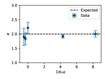
Figure S.1: KHI power-law scaling exponent $\alpha$ in the different interaction regimes, with $\sigma^{*}=A\Delta v^{\alpha}$. The horizontal line denote the expected exponent $\alpha=2$ obtained from Eqs. (1) and (2).

Thermodynamic properties

The thermodynamic properties of the superfluid are obtained from analytical calculations based on the polytropic approximation for trapped gas, for which $\mu=g_{\gamma}n^{\gamma}$, where $\gamma$ is the effective polytropic index $\gamma=\partial\log\mu/\partial\log n$ ^{1, 2}. In the BEC limit, $\gamma=1$, while at unitarity and in the BCS limit, $\gamma=2/3$. Within this approximation, the chemical potential and the Fermi energy take the form ³:

$$\mu_{0}=\left[\frac{\Gamma(\frac{1}{\gamma}+\frac{3}{2})}{\pi^{3/2}\Gamma(\frac{1}{\gamma}+1)}\frac{\sqrt{M/2}\,\omega_{z}Ng_{\gamma}^{1/\gamma}}{R_{\mathrm{e}}^{2}-R_{\mathrm{i}}^{2}}\right]^{\frac{2\gamma}{\gamma+2}},\quad E_{F}=2\hbar\left[\frac{\hbar\omega_{z}N}{m(R_{\mathrm{e}}^{2}-R_{\mathrm{i}}^{2})}\right]^{1/2}$$ (S.1)

where $\Gamma$ is the Gamma function, $g_{\gamma}$ is a pre-factor that depends on the interaction regime: (i) for $(k_{F}a)^{-1}>1$, $g_{\mathrm{BEC}}=4\pi\hbar^{2}a_{M}/M$ with $a_{M}=0.6\,a$, $M=2m$, and $m$ is the mass of the ⁶Li atom; (ii) for $(k_{F}a)^{-1}<-1$, $g_{\mathrm{BCS}}=\frac{\hbar^{2}}{2m}(6\pi^{2})^{2/3}$; (iii) for $|(k_{F}a)^{-1}|<1$, $g_{\mathrm{UFG}}=\xi_{B}\frac{\hbar^{2}}{2m}(6\pi^{2})^{2/3}$, where $\xi_{B}$ is the Bertsch parameter taking the value $\xi_{B}\simeq 0.37$ at unitarity for $T=0$ ². The Fermi wave number (see main text) is $k_{F}=\sqrt{2m\,E_{F}/\hbar^{2}}$.

Speed of sound

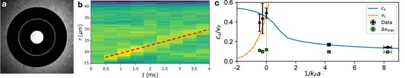
Figure S.2: a, Image of the optical potential projected onto the atomic sample after being shaped by the DMD. b, Density wave propagating in the radial direction after abruptly enlarging and restoring the inner radius of the ring trap by $1.2(2)\text{\,}\mu\mathrm{m}$. c, Black circles correspond to the measured propagation velocity of the density wave as a function of the interaction parameter. Green square symbols correspond to the maximum relative velocity $\Delta v_{max}$ at the interface explored in this work. The solid lines display the expected speed of sound $c_{s}/v_{F}$ in the BEC and crossover regimes (see text). The dashed line corresponds to the critical velocity for pair breaking in the BCS regime ⁴.

We measured the speed of sound by preparing the system in the same ring geometry of Fig. S.2a without the optical barrier separating the ring in two regions. We excite a sound wave propagating along the radial direction by abruptly enlarging and subsequently restoring the inner radius of the box potential. This procedure creates a density burst that travels at constant velocity along the radial direction toward the external radius. We measured the speed of sound $c_{s}$ by fitting the perturbed radial density profile with a Gaussian function, as shown in Fig. S.2b. The measured speed of propagation is reported in Fig. S.2c. To calculate the speed of sound analytically, we calculate $c_{s}=\sqrt{\frac{n}{M}\frac{\partial\mu}{\partial n}}=\sqrt{\gamma\mu/M}$, and take the ratio with the Fermi velocity $v_{F}=\hbar k_{F}$. In the BEC limit and for our geometry, the ratio $c_{s}/v_{F}$ can be expressed analytically in terms of $k_{F}a$ and is given by $\frac{c_{s}}{v_{F}}=\left(\frac{3k_{F}a_{M}}{2^{13/2}}\right)^{1/3}$, and for the BCS and crossover regimes as $\frac{c_{s}}{v_{F}}=\sqrt{{1\over 3}\xi^{3/4}}$, where we assumed $\xi\equiv\xi(k_{F}a)$ at $T=0$ ⁵. The expected behavior of $\frac{c_{s}}{v_{F}}$ is shown in Fig. S.2c as a solid line. For $1/k_{F}a<0$, the measured speed is below the expected speed of sound. However, the measured propagation speed agrees with Leggett 3D homogeneous critical velocity for superfluid pair breaking ⁴, suggesting this method fails to capture the speed of sound in the BCS regime. Nonetheless, the critical velocity for superfluid pair breaking is above the range of superfluid tangential velocities explored in this work.

Quasi-2D vortex dynamics

The vertical confinement provided by the $\mathrm{TEM_{1,0}}$ laser beam is such that in the BEC regimes the ratio $\mu/(\hbar\omega_{z})\gtrapprox 1.5$, and in the UFG and BCS regimes $E_{F}/(\hbar\omega_{z})\approx 6$; making the system collisionally three dimensional. However, vortex dynamics behave as a quasi-two-dimensional system since only a few Kelvin modes can be populated. In fact, the standard Kelvin dispersion ^{6, 7} is:

$$\omega(k)=-\frac{\hbar k^{2}}{2M}\log\left(\xi k\right),$$ (S.2)

where $\xi$ is the healing length. Due to geometrical restrictions ⁷, only modes with wavelength larger than the healing length can be effectively populated in a superfluid. Under our experimental condition, this translates into the fact that only the lowest wavenumber Kelvin mode with $k=\pi/R_{z}$ can be populated in the BEC regime, where $R_{z}=\sqrt{2\mu/(M\omega_{z}^{2})}$ is the Thomas-Fermi radius in the $z$-direction. On the other hand, in the UFG and BCS regimes, due to higher Thomas-Fermi radius and smaller healing length, only the first three Kelvin modes with $k_{n}=(\pi+2\pi n)/R_{z}$ can be populated. Anyway, in all the interaction regimes explored in this work, the number of possibly populated Kelvin modes remains so small that we can assume a 2D dynamics of the vortex motion.

Preparation of the vortex necklace

We remove the circular barrier (Fig. S.2a) between the two rings by lowering its intensity using a sequence of 15 different DMD patterns. To obtain a clear initial condition of the vortex crystal and to prevent the formation of other excitation in the system ⁸, we set the duration of the barrier removal to $\tau=$28\text{\,}\mathrm{m}\mathrm{s}$$.

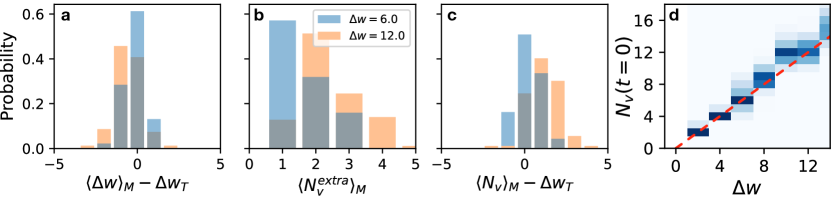
Figure S.3: a, Infidelity in creating the target circulation state state, $\langle\Delta w\rangle_{M}-{\Delta w}_{T}$. b, Number of spurious vortices observed before removing the optical barrier, and c, Deviation of the total number of vortices from the target state, $\langle N_{v}\rangle_{M}-\Delta w_{T}$. All three panels were generated from 100 experimental repetitions for each of the two target states $\Delta w_{T}=6,12$ (blue and orange, respectively). d, Total number of vortices detected after removing the barrier, $t=0$ of vortex dynamics, as a function of the imprinted winding number difference $\Delta w_{T}$. The red dashed line is the identity line, $N_{v}=\Delta w$.

After the complete barrier removal, we observe the creation of a vortex necklace with a number of vortices given by the relative circulation $\Delta w$, as illustrated in Fig. 2a. The phase imprinting method allows to excite circulation states in the two superfluids in a highly reproducible way, but experimental imperfections can lead to shot-to-shot fluctuations in the circulation state of the rings. This leads to fluctuations in the initial configuration of vortices, which we estimate by analyzing the statistics of the relative circulation and vortex number in datasets of 100 experimental realizations on a BEC superfluid at $1/k_{F}a_{s}=4.1(1)$. Figure S.3a shows the distribution of the measured relative circulation between the two rings $\langle\Delta w\rangle_{M}$ with respect to the target $\Delta w_{T}$, measured from interferograms acquired before removing the circular barrier for $\Delta w_{T}=6$ and $\Delta w_{T}=12$. In Fig. S.3b, the number of spurious vortices introduced by the phase-imprinting protocol is displayed, measured from the TOF expansion of the two rings before the barrier removal. Finally, Fig. S.3c shows the distribution of the total number of vortices in the superfluid detected in the TOF expansion after removing the circular barrier. Despite the high reliability in producing the desired circulation states in the two rings(Fig. S.3a), we observe that the distribution of the total number of vortices detected after the barrier removal is augmented and broadened by the presence of spurious vortices. This leads to residual fluctuations of the initial configurations of the vortex necklace (Fig. S.3d), which determine the experimental uncertainty on the initial relative velocity $\Delta v$ (see horizontal error bars in Figs. 3f,g). They also contribute to the experimental noise on the extracted exponential growth rate for a given $\Delta w$.

S.2 Numerical Methods

S.2.1 Gross-Pitaevskii simulations

In the BEC regime, at $T=0$, we simulate our system by solving the three-dimensional Gross-Pitaevskii (GP) equation

$$i\hbar\frac{\partial\psi(\bm{r},t)}{\partial t}=\left[-\frac{\hbar^{2}}{2M}\nabla^{2}+V(\bm{r},t)+gn(\bm{r},t)\right]\psi(\bm{r},t),$$ (S.3)

where $V(\mathbf{r},t)$ is the external potential, $gn(\bm{r},t)$ is the mean-field potential due to the interaction strength $g=4\pi\hbar^{2}a_{M}/M$, the density is $n(\bm{r},t)=\int|\psi(\bm{r},t)|^{2}d^{3}\bm{r}$, and $\int n(\bm{r},t)d^{3}\bm{r}=N$ is the total number of molecules. In particular, the expression for the external potential we employed is:

$$V(r_{\perp},z,t)=V_{G}(t)e^{-2\frac{(r_{\perp}-R_{0})^{2}}{\sigma^{2}}}+V_{r}\left[\tanh\left(\frac{r_{\perp}-R_{e}}{\epsilon}+1\right)+\tanh\left(\frac{R_{i}-r_{\perp}}{\epsilon}+1\right)\right]+\frac{1}{2}M(\omega^{2}_{x}x^{2}+\omega^{2}_{y}y^{2}+\omega^{2}_{z}z^{2}),$$ (S.4)

where $r_{\perp}\equiv\sqrt{x^{2}+y^{2}}$, $V_{G}(t)$ and $\sigma$ are the height and the size of the circular Gaussian barrier located at a distance $R_{0}=(R_{i}+R_{e})/2$ from the center in $xy$ plane, and $V_{r}$ and $\epsilon$ are the height and the stiffness of the ring potential in the $xy$ plane limited by internal and external radii $R_{i}$ and $R_{e}$ respectively. The simulation parameters are $a_{M}=1010\,a_{0}$, $N=3\times 10^{4}$. We used a grid of equal size along $x$ and $y$-directions equal to $\left[-60,60\right]\mu$m and $\left[-10,10\right]\mu$m along $z$ axis, based on up to $384\times 384\times 32$ grid points. The harmonic potential frequencies are the same as in the experiment, $\omega_{x}=\omega_{y}=2\pi\times 2.5$ Hz and $\omega_{z}=2\pi\times 396$ Hz. The parameters of the ring potential are $V_{r}/h=2500$ Hz, $\epsilon=1.5$ $\mu$m, $R_{i}=10$ $\mu$m and $R_{e}=45$ $\mu$m respectively. The barrier size (FWHM) is $\sigma=1.4$ $\mu$m, whereas its height is linearly decreased in time during the barrier removal, starting from the initial value of $V_{G}(t=0)=V_{0}=h\times 5000$ Hz.

We first compute the ground-state of the condensate (with the circular barrier at $V_{0}$) by numerically minimizing the GP energy functional corresponding to Eq. (S.3) by means of a conjugate gradient algorithm ^{9, 10}. The ground-state chemical potential is $\mu/h=887$ Hz. Then, we imprint an opposite circulation in the two rings, adding a phase term $\exp(\pm iw\theta)=\exp[\pm iw\arctan(y/x)]$ in the outer (+) and inner (-) ring, respectively, being $w$ the integer winding number. This phase imprinting results in an opposite velocity field in each of the two rings with $v=\pm\hbar/M\nabla\theta=\pm\hbar w/(Mr_{\perp})$. The dynamical evolution is then triggered by linearly lowering the height $V_{G}(t)$ of the internal barrier at 28 ms, as done in the experiment. At the end of this phase, $N_{v}=\Delta w$ vortices are nucleated at $r_{\perp}=R_{0}$ forming a regular array with angular periodicity $\Delta\theta=2\pi/N_{v}$.

S.2.2 Finite-temperature kinetic model

At finite temperature, the system is partially condensed, and its wavefunction can be written as the sum of condensate and thermal components. Here, we use the collisionless Zaremba-Nikuni-Griffin model ^{11, 12, 13, 14} (cZNG) to investigate the effect of the thermal component. This model has already been successfully applied in the study of different phenomena such as the collective modes ^{15, 16, 17, 18}, soliton and vortex dynamics ^{19, 20, 21, 22, 17}. The condensate wavefunction $\psi$ evolves according to the generalized Gross-Pitaevskii equation:

$$i\hbar\frac{\partial\psi(\bm{r},t)}{\partial t}=\left[-\frac{\hbar^{2}\nabla^{2}}{2M}+V(\bm{r},t)+g(n(\bm{r},t)+2n_{\mathrm{th}}(\bm{r},t))\right]\psi(\bm{r},t)\;,$$ (S.5)

which includes an additional term with respect to the Eq. (S.3): the mean-field potential of the thermal cloud ($2gn_{\mathrm{t}h}$ where $n_{\mathrm{th}}$ is the thermal cloud density). The thermal cloud dynamics is instead described through the phase-space distribution function $f$, which satisfies the collisionless Boltzmann equation:

$$\frac{\partial f}{\partial t}+\frac{\mathbf{p}}{M}\cdot\nabla_{\mathbf{r}}f-\nabla_{\mathbf{r}}V^{\rm eff}_{\rm th}\cdot\nabla_{\mathbf{p}}f=0$$ (S.6)

where $V^{\rm eff}_{\rm th}=V+2g(n+n_{\rm th})$ is the generalized mean-field potential felt by the thermal particles. The thermal cloud density instead is found as $n_{\rm th}=1/(2\pi\hbar)^{3}\int d\mathbf{p}~{}f(\mathbf{p},\mathbf{r},t)$). These two equations are solved self-consistently in a grid of equal size along the $x$ and $y$ directions, equal to $\left[-106,106\right]\mu$m, and to $\left[-22,22\right]\mu$m along the $z$ axis, based on $768\times 768\times 160$ grid points. The total particle number is equal to $N=3\times 10^{4}$.

We first find the condensate equilibrium density by solving the time-independent generalized GP equation:

$$\mu\psi_{0}=\left(-\frac{\hbar^{2}}{2M}\nabla^{2}+V+g(n_{0}+2n^{0}_{\mathrm{th}})\right)\psi_{0},$$ (S.7)

with $n_{0}$ and $n_{0}^{\mathrm{th}}$ being the equilibrium condensate and thermal density, respectively, in the presence of the circular Gaussian barrier. The initial thermal cloud density Ansatz is based on a Gaussian profile obtained for a certain temperature ¹¹. Then, we imprint a phase on the initial condensate wavefunction, as it was done for $T=0$ GP simulations, having opposite signs in the outer (+) and inner (-) rings. After that, the generalized GP equation and the Boltzmann equation are solved self-consistently in order to describe the system dynamics, in the presence of a time-dependent circular barrier whose potential height is removed in 28 ms. Due to the repulsive interaction between condensate and thermal particles, the thermal density $n^{\rm th}$ is maximum where the condensate density $n^{\rm BEC}$ is minimum, as it occurs e.g. at the barrier position, at the edges of the condensate and at the vortex cores.

S.2.3 Time evolution and stability analysis from the numerical results

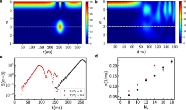
Figure S.4: Heat map of the angular structure factor $S(m,t)$ for the $\Delta w=6$ configuration for: a, $T=0$ (GP) and b, $T\simeq 0.4T_{c}$ (cZNG). The dashed line corresponds to $m=\Delta w/2$, whose amplitudes in logarithmic scales as a function of time for both temperatures are shown in panel c. d, Comparison between the growth rate extracted at $T=0$ and $T\simeq 0.4T_{c}$ as a function of the number of vortices.

From the simulations performed either using the GP equations for the $T=0$ case, or the cZNG model for the $T\neq 0$ case, we extract the density profile integrated along $z$. Then we identify the positions of the vortices ad different evolution times $t$, from which we calculate the structure factor $S(m,t)$ for different modes $m$. The result is shown in Fig. S.4 a for the case of $\Delta w=6$ (indicated by the color). Fig. S.4c, shows the time-dependence of the structure factor for the mode $m=\Delta w/2$ mode both for the $T=0$ (black) and $T=53nK$ (red) which is characterized by an initial exponential growth. Similarly, Fig. S.4 b shows the behaviour of the structure factor at temperature $T=53\,\mbox{nK}\simeq 0.4\,T_{c}$, close to the experimental value. We first observe that similar to the experimental results, at finite temperature, the growth of the $m=3$ mode amplitude starts almost immediately after the vortex array is generated, while at $T=0$ the instability starts much later. Furthermore, at a finite temperature, more modes are populated. We then extract the growth rate of the instability, and this procedure is repeated for different initial velocities, with the results shown in Fig. S.4d. Interestingly, even though the starting time of the instability and the population of different modes are strongly affected by the presence of the thermal cloud, the growth rate of the $m=\Delta w/2$ mode turns out to be only slightly affected, being in average larger than the one at $T=0$. We also note that at longer time evolution, the presence of the thermal cloud significantly affects the vortices dynamics, consistent with the results of ^{20, 21}.

Some additional tests have been performed to prove the stability of the GP results presented in this work. We verified that by doubling or halving the number of particles $N$ or the width of the internal barrier $\sigma$, the growth rates do not change. We also included in the GP simulations some noise in the density distribution of the ground state of the BEC. This noise term only affects the time when the instability starts without changing the growth rates of the most unstable mode. Moreover, cZNG simulations show that fixing the condensate number of the finite temperature case to be the same as the simulation at $T=0$ provides a similar growth rate, opposite to what is found in a Josephson junction ¹⁸ where the superfluid dynamics strongly depends on the condensate number.

Finally, we tried to include in the simulation an imperfect phase imprinting. This has been done by adding a phase to the ground state wavefunction distributed around a mean value $2\pi w$ with fluctuations smaller than $\pi$. This phase imprinting leads to the creation of density waves, which affect the dynamics of the vortex crystal. However, by averaging on different realizations, we found that the most unstable mode’s growth rate has a value that is only $18\%$ smaller than the one of the clean configuration. Nevertheless, we do not exclude that the presence of additional vortices due to the experimental imprinting techniques could have a larger effect on the observed growth rates.

S.2.4 Thickness of the interface layer and correction factor

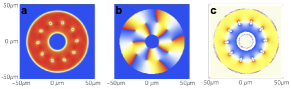
Figure S.5: Gross-Pitaevskii simulations. a, Density distribution $n(x,y,0)$; b, phase distribution$\phi(x,y,0)$; c, angular velocity distribution $v_{\theta}(x,y,0)$ for the case $\Delta w=10$ at $t=0$.

To estimate the interface thickness $\delta$ in Eq. (2), we analyzed the results of the GP simulations in the following way. From the phase $\phi$ of the condensate wavefunction, we numerically compute the velocity field as $v=\hbar/M\nabla\phi$. In Fig. S.5, we show, from left to right, the density distribution $n(x,y,0)$, the phase $\phi(x,y,0)$, and the tangential velocity field $v_{\theta}(x,y,0)$, for the case with $\Delta w=10$ at $t=0$, namely immediately after the removal of the circular barrier. Considering that the tangential velocity field $v_{\theta}$ changes sign at $r_{\perp}=R_{0}$, to extract the width of the interface layer between the two regions, we fit the radial velocity profile with the function $v_{\theta}(r_{\perp})=a\tanh\left[(r_{\perp}-R_{0})/\delta(\theta)\right]/r_{\perp}$. The behaviour of $v_{\theta}(r_{\perp})$ is shown in Fig. S.6a for different values of $\theta$ between two adjacent vortices. The value of $\delta(\theta)$ extracted from the fit is shown in Fig. S.6b. The interface thickness exhibits a sinusoidal behavior with minima in correspondence with the vortex cores and maxima in the middle of each vortex pair.

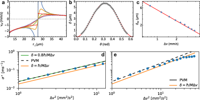
Figure S.6: a, Plot of $v_{\theta}$ for different angular positions between two adjacent vortices for the case $N_{v}=10$. The vertical gray dashed line corresponds to $r=R_{0}$, and the dashed red line represents the imprinted velocity in the two rings with modulus $\hbar N_{v}/(2Mr_{\perp})$. b, Values of the interface half-width $\delta$ (gray data point) for different angular positions between two consecutive vortices located at $\theta=0$ rad and $\theta=0.63$ rad ($N_{v}$=10). This behaviour is fitted with a sinusoidal function $\delta=a\cos(N_{v}\theta)+b$ (red line) to extract the mean value $\delta_{\text{av}}=b$. c, Values of $\delta_{\text{av}}$ as a function of $\Delta v$, plotted together with the expected behavior $\delta=\hbar/(M\Delta v)$ (red line). d–e, Extracted growth rate from the GP simulations (blue circles) as a function of $\Delta v$ for the experimentally explored velocities (d), and all simulated velocities (e). The PVM maximum growth rate is shown as a black dashed line, while the solid lines correspond to Rayleigh’s formula for the maximum growth rate with $\eta=0.8$ (green line) and $\eta=1$ (orange line).

We define the effective value of the interface half-width $\delta_{\text{av}}$ as the average value of $\delta(\theta)$, and extract it by fitting such quantity with a sinusoidal function $\delta=a\cos(N_{v}\theta)+\delta_{\text{av}}$. In Fig. S.6c we report the obtained values of $\delta_{\text{av}}$ as a function of $\Delta v=\hbar\Delta w/(MR_{0})$. A similar study of the effective thickness of the interface can be performed within the PVM. As commented in the Methods, the equation of motion of a linear array of equispaced vortices can be analytically solved in a 2D space $x-y$ without boundaries, providing Eq. (3) of the main text for the velocity field. Plotting $v_{x}(x_{0},y)$ for various $x_{0}\in[-0.5d_{v},\,0.5\,d_{v}]$ between two neighboring vortices provides similar trends of Fig. S.6 a-b. We then employ the same procedure used to extract $\delta_{\text{av}}$ from the GP results for the PVM prediction, obtaining results in agreement with those of GP simulations. In particular, the estimated average interface thickness with both methods is well in agreement with the formula $\delta_{\text{av}}=\hbar/(M\Delta v)$, which we plot in Fig. S.6c as a red line.

On the other hand, Rayleigh’s formula involves a linearly varying velocity between the two merging superfluids. We account for this difference by introducing an effective interface thickness $\delta=\eta\hbar/(M\Delta v)$, where $\eta$ is a phenomenological parameter of the order of $1$. We then fix the value of $\eta$ asking that the expressions of the most unstable mode under Rayleigh’s formula [Eq. (2)] and PVM are the same, namely:

$$\sigma_{R}^{*}(k,\Delta v)=\left(\frac{\sqrt{e^{-2\eta}-(\eta-1)^{2}}}{\eta}\right)\frac{M\Delta v^{2}}{4\hbar}=\sigma_{PVM}(k^{*},\Delta v)=\frac{1}{2}\frac{M\Delta v^{2}}{4\hbar}.$$ (S.8)

For the two expressions to be the same, we have to fix $\left(\sqrt{e^{-2\eta}-(\eta-1)^{2}}\right)/\eta=\frac{1}{2}$, yielding the value of $\eta\approx 0.80465$.

Finally, we verified that such a value of $\delta$ is also consistent with GP simulation results of the most unstable mode $\sigma_{\text{GP}}$. In particular, in Fig. S.6e, we report the values of $\sigma_{\text{GP}}$ as extracted from GP simulations (symbols) and compare it with the one given by Eq. (S.8) with $\eta=1$ (orange line) and $\eta=0.8$ (green line). The latter is observed to well reproduce the GP results for low velocities, whereas for larger ones $\eta=1$ matches the GP results better. The transition between these two regimes happens at velocities where the PVM is no longer applicable, i.e., when the inter-vortex distance is in the same order of magnitude as the healing length. The transition approximately occurs when $h/(M\Delta v)\approx 15~{}\xi$, with the associated velocity limit of $\Delta v=h/(15\,\xi M)\approx 3.16$ mm/s, or $\Delta w\approx 16$. For these reasons, we use the value $\eta\approx 0.8$ for $\Delta w<16$ for all the measurements reported in this work.

S.2.5 Point-Vortex Model (PVM) simulations

We consider a two-dimensional fluid containing $N_{v}$ point vortices with quantized circulations $\Gamma=h/M$. When the inter-vortex separation is greater than a few healing lengths, vortices are advected by the velocity field created by other vortices. The equation of motion of each vortex is $d\vec{r}_{i}/dt=\vec{v_{i}}^{0}$, where $\vec{v_{i}}^{0}$ is the velocity field created by all the other vortices. When considering the ring geometry, $\vec{v_{i}}^{0}$ must take into account the boundary conditions, namely that the flow must have a zero radial component at both the internal ($R_{i}$) and external ($R_{e}$) radii. We include the boundary conditions by using the method of image vortices ²³:

$$\vec{v_{i}}^{0} =\frac{\Gamma}{2\pi}\sum_{i\neq j}^{N_{v}}\kappa_{j}\hat{z}\times\frac{\vec{r}_{i}-\vec{r}_{j}}{\left|\vec{r}_{i}-\vec{r}_{j}\right|^{2}}+\frac{1}{2}\left(\frac{\Gamma}{2\pi}\sum_{j=1}^{N_{v}}\kappa_{j}\hat{z}\times\frac{\vec{r}_{i}-\vec{0}}{\left|\vec{r}_{i}-\vec{0}\right|^{2}}\right)$$ (S.9)

$$+\frac{\Gamma}{2\pi}\sum_{j=1}^{N_{v}}\sum_{n=1}^{\infty}\kappa_{j}\hat{z}\times\left(\frac{\vec{r}_{i}-\left(\frac{R_{e}}{R_{i}}\right)^{2n}\vec{r}_{j}}{\left|\vec{r}_{i}-\left(\frac{R_{e}}{R_{i}}\right)^{2n}\vec{r}_{j}\right|^{2}}+\frac{\vec{r}_{i}-\left(\frac{R_{i}}{R_{e}}\right)^{2n}\vec{r}_{j}}{\left|\vec{r}_{i}-\left(\frac{R_{i}}{R_{e}}\right)^{2n}\vec{r}_{j}\right|^{2}}\right)$$

$$-\frac{\Gamma}{2\pi}\sum_{j=1}^{N_{v}}\sum_{n=0}^{\infty}\kappa_{j}\hat{z}\times\left(\frac{\vec{r}_{i}-\left(\frac{R_{e}}{R_{i}}\right)^{2n}\left(\frac{R_{e}^{2}}{|\vec{r}_{j}|^{2}}\right)\vec{r}_{j}}{\left|\vec{r}_{i}-\left(\frac{R_{e}}{R_{i}}\right)^{2n}\left(\frac{R_{e}^{2}}{|\vec{r}_{j}|^{2}}\right)\vec{r}_{j}\right|^{2}}+\frac{\vec{r}_{i}-\left(\frac{R_{i}}{R_{e}}\right)^{2n}\left(\frac{R_{i}^{2}}{|\vec{r}_{j}|^{2}}\right)\vec{r}_{j}}{\left|\vec{r}_{i}-\left(\frac{R_{i}}{R_{e}}\right)^{2n}\left(\frac{R_{i}^{2}}{|\vec{r}_{j}|^{2}}\right)\vec{r}_{j}\right|^{2}}\right)$$

We solve the equations of motions for the vortex necklace configuration in the ring with the Runge-Kutta method of fourth order. From the obtained trajectories of the vortices, $\vec{r}_{i}(t)$ we compute the normalized angular structure factor $s(m,t)$.

References

- von Helmholtz [1868] H. von Helmholtz, Über discontinuierliche flüssigkeits-bewegungen [On the discontinuous movements of fluids], Monats. Königl. Preuss. Akad. Wiss. Berlin 23, 215 (1868).
- Sir William Thomson F. R. S. [1871] Sir William Thomson F. R. S., XLVI. Hydrokinetic solutions and observations, The London, Edinburgh, and Dublin Philosophical Magazine and Journal of Science 42, 362 (1871).
- Luce et al. [2018] H. Luce, L. Kantha, M. Yabuki, and H. Hashiguchi, Atmospheric Kelvin–Helmholtz billows captured by the MU radar, lidars and a fish-eye camera, Earth, Planets and Space 70, 162 (2018).
- Fukao et al. [2011] S. Fukao, H. Luce, T. Mega, and M. K. Yamamoto, Extensive studies of large-amplitude Kelvin-Helmholtz billows in the lower atmosphere with VHF middle and upper atmosphere radar, Quarterly Journal of the Royal Meteorological Society 137, 1019 (2011).
- Li and Yamazaki [2001] H. Li and H. Yamazaki, Journal of Oceanography 57, 709 (2001).
- Smyth and Moum [2012] W. Smyth and J. Moum, Ocean mixing by Kelvin-Helmholtz instability, Oceanography 25, 140 (2012).
- McNally et al. [2012] C. P. McNally, W. Lyra, and J.-C. Passy, A well-posed kelvin–helmholtz instability test and comparison, Astrophys. J. 201, 18 (2012).
- Klaassen and Peltier [1985] G. P. Klaassen and W. R. Peltier, The onset of turbulence in finite-amplitude Kelvin–Helmholtz billows, Journal of Fluid Mechanics 155, 1 (1985).
- Mashayek and Peltier [2012] A. Mashayek and W. R. Peltier, The ‘zoo’ of secondary instabilities precursory to stratified shear flow transition. part 2 the influence of stratification, Journal of Fluid Mechanics 708, 45 (2012).
- Thorpe [1987] S. A. Thorpe, Transitional phenomena and the development of turbulence in stratified fluids: A review, Journal of Geophysical Research 92, 5231 (1987).
- Thorpe [2012] S. A. Thorpe, On the kelvin–helmholtz route to turbulence, Journal of Fluid Mechanics 708, 1 (2012).
- Thorpe [2002] S. A. Thorpe, The axial coherence of Kelvin–Helmholtz billows, Quarterly Journal of the Royal Meteorological Society 128, 1529 (2002).
- Drazin and Reid [2004] P. G. Drazin and W. H. Reid, Hydrodynamic Stability (Cambridge University Press, Cambridge, 2004) pp. 1–31.
- Charru [2011] F. Charru, Hydrodynamic Instabilities (Cambridge University Press, 2011).
- Aref [1995] H. Aref, On the equilibrium and stability of a row of point vortices, Journal of Fluid Mechanics 290, 167 (1995).
- Havelock [1931] T. Havelock, LII. The stability of motion of rectilinear vortices in ring formation, The London, Edinburgh, and Dublin Philosophical Magazine and Journal of Science 11, 617 (1931).
- Johnstone et al. [2019] S. P. Johnstone, A. J. Groszek, P. T. Starkey, C. J. Billington, T. P. Simula, and K. Helmerson, Evolution of large-scale flow from turbulence in a two-dimensional superfluid, Science 364, 1267 (2019).
- Gauthier et al. [2019] G. Gauthier, M. T. Reeves, X. Yu, A. S. Bradley, M. A. Baker, T. A. Bell, H. Rubinsztein-Dunlop, M. J. Davis, and T. W. Neely, Giant vortex clusters in a two-dimensional quantum fluid, Science 364, 1264 (2019).
- Barenghi et al. [2014] C. F. Barenghi, L. Skrbek, and K. R. Sreenivasan, Introduction to quantum turbulence, Proc. Natl. Acad. Sci. U.S.A. 111, 4647 (2014).
- Kobyakov et al. [2014] D. Kobyakov, A. Bezett, E. Lundh, M. Marklund, and V. Bychkov, Turbulence in binary Bose-Einstein condensates generated by highly nonlinear Rayleigh-Taylor and Kelvin-Helmholtz instabilities, Phys. Rev. A 89, 013631 (2014).
- Neely et al. [2013] T. W. Neely, A. S. Bradley, E. C. Samson, S. J. Rooney, E. M. Wright, K. J. H. Law, R. Carretero-González, P. G. Kevrekidis, M. J. Davis, and B. P. Anderson, Characteristics of two-dimensional quantum turbulence in a compressible superfluid, Phys. Rev. Lett. 111, 235301 (2013).
- Reynolds [1883] O. Reynolds, XXIX. An experimental investigation of the circumstances which determine whether the motion of water shall be direct or sinuous, and of the law of resistance in parallel channels, Philos. Trans. R. Soc. Lond. 174, 935 (1883).
- Thorpe [1968] S. A. Thorpe, A method of producing a shear flow in a stratified fluid, Journal of Fluid Mechanics 32, 693 (1968).
- Kent [1969] G. I. Kent, Transverse Kelvin-Helmholtz instability in a rotating plasma, Physics of Fluids 12, 2140 (1969).
- Thorpe [1971] S. A. Thorpe, Experiments on the instability of stratified shear flows: miscible fluids, Journal of Fluid Mechanics 46, 299 (1971).
- Sullivan and List [1993] G. D. Sullivan and E. J. List, An experimental investigation of vertical mixing in two-layer density-stratified shear flows, Dynamics of Atmospheres and Oceans 19, 147 (1993).
- Shearer and Früh [1999] E. Shearer and W.-G. Früh, Kelvin-helmholtz instability in a continuously forced shear flow, Physics and Chemistry of the Earth, Part B: Hydrology, Oceans and Atmosphere 24, 487 (1999).
- Bennemann and Ketterson [2014] K.-H. Bennemann and J. B. Ketterson, Novel Superfluids: Volume 2 (Oxford University Press, 2014).
- Bloch et al. [2008] I. Bloch, J. Dalibard, and W. Zwerger, Many-body physics with ultracold gases, Rev. Mod. Phys. 80, 885 (2008).
- Korshunov [2002] S. E. Korshunov, Analog of Kelvin-Helmholtz instability on a free surface of a superfluid liquid, J. Exp. Theor. Phys. 75, 423 (2002).
- Volovik [2002] G. E. Volovik, On the Kelvin-Helmholtz instability in superfluids, J. Exp. Theor. Phys. 75, 418 (2002).
- Takeuchi et al. [2010] H. Takeuchi, N. Suzuki, K. Kasamatsu, H. Saito, and M. Tsubota, Quantum Kelvin-Helmholtz instability in phase-separated two-component Bose-Einstein condensates, Phys. Rev. B 81, 094517 (2010).
- Suzuki et al. [2010] N. Suzuki, H. Takeuchi, K. Kasamatsu, M. Tsubota, and H. Saito, Crossover between Kelvin-Helmholtz and counter-superflow instabilities in two-component Bose-Einstein condensates, Phys. Rev. A 82, 063604 (2010).
- Lundh and Martikainen [2012] E. Lundh and J.-P. Martikainen, Kelvin-Helmholtz instability in two-component Bose gases on a lattice, Phys. Rev. A 85, 023628 (2012).
- Blaauwgeers et al. [2002] R. Blaauwgeers, V. B. Eltsov, G. Eska, A. P. Finne, R. P. Haley, M. Krusius, J. J. Ruohio, L. Skrbek, and G. E. Volovik, Shear flow and Kelvin-Helmholtz instability in superfluids, Phys. Rev. Lett. 89, 155301 (2002).
- Finne et al. [2006] A. P. Finne, V. B. Eltsov, R. Hänninen, N. B. Kopnin, J. Kopu, M. Krusius, M. Tsubota, and G. E. Volovik, Dynamics of vortices and interfaces in superfluid 3He, Rep. Progr. Phys. 69, 3157 (2006).
- Baggaley and Parker [2018] A. W. Baggaley and N. G. Parker, Kelvin-Helmholtz instability in a single-component atomic superfluid, Phys. Rev. A 97, 053608 (2018).
- Giacomelli and Carusotto [2023] L. Giacomelli and I. Carusotto, Interplay of Kelvin-Helmholtz and superradiant instabilities of an array of quantized vortices in a two-dimensional Bose-Einstein condensate, SciPost Phys. 14, 025 (2023).
- Mukherjee et al. [2022] B. Mukherjee, A. Shaffer, P. B. Patel, Z. Yan, C. C. Wilson, V. Crépel, R. J. Fletcher, and M. Zwierlein, Crystallization of bosonic quantum Hall states in a rotating quantum gas, Nature 601, 58 (2022).
- [40] See Supplementary Information.
- Del Pace et al. [2022] G. Del Pace, K. Xhani, A. Muzi Falconi, M. Fedrizzi, N. Grani, D. Hernandez Rajkov, M. Inguscio, F. Scazza, W. J. Kwon, and G. Roati, Imprinting persistent currents in tunable fermionic rings, Phys. Rev. X 12, 041037 (2022).
- Eckel et al. [2014] S. Eckel, F. Jendrzejewski, A. Kumar, C. J. Lobb, and G. K. Campbell, Interferometric measurement of the current-phase relationship of a superfluid weak link, Phys. Rev. X 4, 031052 (2014).
- Rayleigh [1879] L. Rayleigh, On the stability, or instability, of certain fluid motions, Proceedings of the London Mathematical Society s1-11, 57 (1879).
- Warren [1990] B. E. Warren, X-Ray Diffraction, Dover Books on Physics (Dover Publications, Mineola, NY, 1990).
- Griffin et al. [2009] A. Griffin, T. Nikuni, and E. Zaremba, Bose-Condensed Gases at Finite Temperatures (Cambridge University Press, 2009).
- Proukakis et al. [2013] N. Proukakis, S. Gardiner, M. Davis, and M. Szymańska, eds., Quantum Gases: Finite Temperature and Non-Equilibrium Dynamics (Imperial College Press, London, United Kingdom, 2013).
- Kwon et al. [2021] W. J. Kwon, G. D. Pace, K. Xhani, L. Galantucci, A. M. Falconi, M. Inguscio, F. Scazza, and G. Roati, Sound emission and annihilations in a programmable quantum vortex collider, Nature 600, 64 (2021).
- Barresi et al. [2023] A. Barresi, A. Boulet, P. Magierski, and G. Wlazłowski, Dissipative dynamics of quantum vortices in fermionic superfluid, Phys. Rev. Lett. 130, 043001 (2023).
- Sonin [2015] E. B. Sonin, Dynamics of Quantised Vortices in Superfluids (Cambridge University Press, 2015).
- Mehdi et al. [2023] Z. Mehdi, J. J. Hope, S. S. Szigeti, and A. S. Bradley, Mutual friction and diffusion of two-dimensional quantum vortices, Phys. Rev. Res. 5, 013184 (2023).
- Pikovsky and Politi [2016] A. Pikovsky and A. Politi, Lyapunov exponents (Cambridge University Press, Cambridge, England, 2016).
- Babiano et al. [1994] A. Babiano, G. Boffetta, A. Provenzale, and A. Vulpiani, Chaotic advection in point vortex models and two-dimensional turbulence, Physics of Fluids 6, 2465 (1994).
- Haskell and Melatos [2015] B. Haskell and A. Melatos, Models of pulsar glitches, Int. J. Mod. Phys. D 24, 1530008 (2015).
- Price and Rosswog [2006] D. J. Price and S. Rosswog, Producing ultrastrong magnetic fields in neutron star mergers, Science 312, 719 (2006).
- Sachkou et al. [2019] Y. P. Sachkou, C. G. Baker, G. I. Harris, O. R. Stockdale, S. Forstner, M. T. Reeves, X. He, D. L. McAuslan, A. S. Bradley, M. J. Davis, and W. P. Bowen, Coherent vortex dynamics in a strongly interacting superfluid on a silicon chip, Science 366, 1480 (2019).
- Simula et al. [2014] T. Simula, M. J. Davis, and K. Helmerson, Emergence of order from turbulence in an isolated planar superfluid, Phys. Rev. Lett. 113, 165302 (2014).
- Reeves et al. [2022] M. T. Reeves, K. Goddard-Lee, G. Gauthier, O. R. Stockdale, H. Salman, T. Edmonds, X. Yu, A. S. Bradley, M. Baker, H. Rubinsztein-Dunlop, M. J. Davis, and T. W. Neely, Turbulent relaxation to equilibrium in a two-dimensional quantum vortex gas, Phys. Rev. X 12, 011031 (2022).
- Heyl et al. [2022] M. Heyl, K. Adachi, Y. M. Itahashi, Y. Nakagawa, Y. Kasahara, E. J. W. List-Kratochvil, Y. Kato, and Y. Iwasa, Vortex dynamics in the two-dimensional BCS-BEC crossover, Nature Comm. 13, 6986 (2022).
- Henn et al. [2009] E. A. L. Henn, J. A. Seman, G. Roati, K. M. F. Magalhães, and V. S. Bagnato, Emergence of turbulence in an oscillating Bose-Einstein condensate, Phys. Rev. Lett. 103, 045301 (2009).
- Navon et al. [2016] N. Navon, A. L. Gaunt, R. P. Smith, and Z. Hadzibabic, Emergence of a turbulent cascade in a quantum gas, Nature 539, 72 (2016).
Supplemental Information

References

- Heiselberg [2004] H. Heiselberg, Collective modes of trapped gases at the BEC-BCS crossover, Phys. Rev. Lett. 93, 040402 (2004).
- Haussmann and Zwerger [2008] R. Haussmann and W. Zwerger, Thermodynamics of a trapped unitary fermi gas, Phys. Rev. A 78, 063602 (2008).
- Del Pace et al. [2022] G. Del Pace, K. Xhani, A. Muzi Falconi, M. Fedrizzi, N. Grani, D. Hernandez Rajkov, M. Inguscio, F. Scazza, W. J. Kwon, and G. Roati, Imprinting persistent currents in tunable fermionic rings, Phys. Rev. X 12, 041037 (2022).
- Weimer et al. [2015] W. Weimer, K. Morgener, V. P. Singh, J. Siegl, K. Hueck, N. Luick, L. Mathey, and H. Moritz, Critical velocity in the bec-bcs crossover, Phys. Rev. Lett. 114, 095301 (2015).
- Kwon et al. [2020] W. J. Kwon, G. D. Pace, R. Panza, M. Inguscio, W. Zwerger, M. Zaccanti, F. Scazza, and G. Roati, Strongly correlated superfluid order parameters from dc josephson supercurrents, Science 369, 84 (2020).
- Fetter [2004] A. L. Fetter, Kelvin mode of a vortex in a nonuniform Bose-Einstein condensate, Phys. Rev. A 69, 043617 (2004).
- Rooney et al. [2011] S. J. Rooney, P. B. Blakie, B. P. Anderson, and A. S. Bradley, Suppression of kelvon-induced decay of quantized vortices in oblate Bose-Einstein condensates, Phys. Rev. A 84, 023637 (2011).
- Kanai et al. [2019] T. Kanai, W. Guo, and M. Tsubota, Merging of rotating Bose-Einstein condensates, J. Low. Temp. Phys. 195, 37 (2019).
- Press et al. [2007] W. H. Press, S. A. Teukolsky, W. T. Vetterling, and B. P. Flannery, Numerical Recipes: The Art of Scientific Computing, 3rd ed. (Cambridge University Press, USA, 2007).
- Modugno et al. [2003] M. Modugno, L. Pricoupenko, and Y. Castin, Bose-Einstein condensates with a bent vortex in rotating traps, Eur. Phys. J. D 22, 235 (2003).
- Griffin et al. [2009] A. Griffin, T. Nikuni, and E. Zaremba, Bose-Condensed Gases at Finite Temperatures (Cambridge University Press, 2009).
- Jackson and Zaremba [2002a] B. Jackson and E. Zaremba, Modeling Bose-Einstein condensed gases at finite temperatures with N-body simulations, Phys. Rev. A 66, 033606 (2002a).
- Proukakis and Jackson [2008] N. P. Proukakis and B. Jackson, Finite-temperature models of Bose–Einstein condensation, J. Phys. B: At. Mol. Opt. Phys. 41, 203002 (2008).
- Proukakis et al. [2013] N. Proukakis, S. Gardiner, M. Davis, and M. Szymańska, eds., Quantum Gases: Finite Temperature and Non-Equilibrium Dynamics (Imperial College Press, London, United Kingdom, 2013).
- Jackson and Zaremba [2002b] B. Jackson and E. Zaremba, Quadrupole collective modes in trapped finite-temperature Bose-Einstein condensates, Phys. Rev. Lett. 88, 180402 (2002b).
- Jackson and Zaremba [2001] B. Jackson and E. Zaremba, Finite-temperature simulations of the scissors mode in Bose-Einstein condensed gases, Phys. Rev. Lett. 87, 100404 (2001).
- Xhani et al. [2020] K. Xhani, E. Neri, L. Galantucci, F. Scazza, A. Burchianti, K.-L. Lee, C. F. Barenghi, A. Trombettoni, M. Inguscio, M. Zaccanti, G. Roati, and N. P. Proukakis, Critical transport and vortex dynamics in a thin atomic Josephson junction, Phys. Rev. Lett. 124, 045301 (2020).
- Xhani and Proukakis [2022] K. Xhani and N. P. Proukakis, Dissipation in a finite-temperature atomic Josephson junction, Phys. Rev. Res. 4, 033205 (2022).
- Jackson et al. [2007] B. Jackson, N. P. Proukakis, and C. F. Barenghi, Dark-soliton dynamics in Bose-Einstein condensates at finite temperature, Phys. Rev. A 75, 051601 (2007).
- Jackson et al. [2009] B. Jackson, N. P. Proukakis, C. F. Barenghi, and E. Zaremba, Finite-temperature vortex dynamics in Bose-Einstein condensates, Phys. Rev. A 79, 053615 (2009).
- Allen et al. [2013] A. J. Allen, E. Zaremba, C. F. Barenghi, and N. P. Proukakis, Observable vortex properties in finite-temperature Bose gases, Phys. Rev. A 87, 013630 (2013).
- Allen et al. [2014] A. J. Allen, S. Zuccher, M. Caliari, N. P. Proukakis, N. G. Parker, and C. F. Barenghi, Vortex reconnections in atomic condensates at finite temperature, Phys. Rev. A 90, 013601 (2014).
- Martikainen et al. [2001] J.-P. Martikainen, K.-A. Suominen, L. Santos, T. Schulte, and A. Sanpera, Generation and evolution of vortex-antivortex pairs in Bose-Einstein condensates, Phys. Rev. A 64, 063602 (2001).