Abstract

Through modeling the universe as a symplectic 3-brane embedded in the bulk of $\mathcal{N}=2$ five-dimensional ungauged supergravity theory, the entire evolution of the universe can be interpreted from inflation to late-time acceleration without introducing an inflaton nor a cosmological constant. The time dependence of the brane is strongly correlated to the complex structure moduli of the underlying Calabi-Yau submanifold and the bulk effects. The solutions to the field equations are found by exploiting the theory’s symplectic structure where the time evolution is similar to our universe according to the latest data of the Planck mission. Our results present a new explanation for the nature of dark energy mainly based on the topology of the subspace and the existence of a fifth extra dimension.

I Introduction

Cosmological evolution incorporates many mysteries. For instance, we assume with high confidence that our observable universe came to exist in an event known as the Big Bang some $13.842$ billion years ago [1], but little is known about its initial conditions. In other words what caused the Big Bang to happen? Did the universe, in a sense, have any choice about coming to exist? The general theory of relativity (GR) implies that it started with a singularity, but did it? It is also known that shortly after the Big Bang, a period of rapid acceleration; known as ‘inflation,’ caused the universe to expand very rapidly in a very short period [2]. Following a period of the so-called ‘graceful exit,’ decelerated expansion occurred. This last is the only epoch whose reasons are fully understood: namely the gravitational interaction of the universe on itself following the standard Friedmann equations. Then, roughly around our current time, a period of slow accelerated expansion started, as discovered by the Supernova Cosmology Project [3], and the Supernova Search Team [4]. The ‘dark energy’ refers to the mysterious source of negative pressure which drives the universe for that expansion. In Einstein’s gravitational theory this energy is accounted for by adding a term to the field equation called the cosmological constant ($\Lambda$) [5]. But unfortunately, the observational constraint on the density of the dark energy is $|\rho_{\Lambda}|<10^{-27}~{}\text{kg/m}^{3}\sim 10^{-47}~{}\text{GeV}^{4}$ [6, 7], while the cosmological constant in GR receives many corrections from the quantum vacuum energy whose energy density ($\rho_{th}$) theoretically exceeds the observational bound by at least 120 orders of magnitude. That means $\Lambda$ is of order $\sim 9.9834\times 10^{-120}~{}\Lambda_{th}$.

On the other hand, in recent years much attention has been drawn to five-dimensional $\mathcal{D}=5$ $\mathcal{N}=2$ supergravity theories for many reasons. For instance, they are so relevant to the AdS/CFT correspondence [8], and they have a vital role in M-theory compactification on the Calabi-Yau manifold with cosmological applications [9]. There are many proposed models of ‘brane-cosmology’ in which the universe is considered as a 3-brane (supersymmetric or non-supersymmetric) embedded in a higher dimensional spacetime [10]. Some of these models explain inflation based on the existence of a scalar field in the early universe called the ‘inflaton’ [11]. Other models focus on the late-time acceleration of the universe [12]. However, it seems that studies of the whole cosmic evolution of the universe by a single model are rare.

In this paper, we aim to explain the entire cosmic history of the universe during its different acceleration phases from inflation till the present accelerated expansion. We model the universe as a symplectic 3-brane embedded in the bulk of $\mathcal{N}=2$ $\mathcal{D}=5$ supergravity that has been produced from the dimensional reduction of $\mathcal{D}=11$ $\mathcal{N}=1$ supergravity over Calabi-Yau 3-fold [13]. The brane is filled by dust matter and radiation, whilst its cosmological constant vanishes, and only the extra fifth dimension has a cosmological constant called ($\tilde{\Lambda}$). When we numerically solve the modified field equations, we find that the flow norm of the moduli of the complex structure of the underlying Calabi-Yau manifold starts with very large values and decays rapidly (without any imposed initial conditions) [14, 15]. We also find that there is a strong correlation between the moduli and the dynamics of the brane, especially since it is correlated to an early epoch of rapid expansion, i.e., inflation. Whereas the late-time acceleration occurs because of the presence of the bulk’s cosmological constant mediated by the moduli flow norm. The solutions are BPS (Bogomol’nyi-Prasad-Sommerfield) [16] in the sense they partially preserve supersymmetry, and they are related to the initial conditions of the brane-universe. To fit the recent observations of the $\Lambda$CDM model [17], the bulk should be a de Sitter space with a tiny positive cosmological constant $(0.02<\tilde{\Lambda}<0.03)~{}[\text{Gyr}^{-2}]$. In other words, an expanding universe does not need a cosmological constant on the brane to explain its late-time acceleration nor the so-called inflaton to describe the early-time inflation. The whole cosmic evolution of the universe can be explained by topological effects and the existence of an extra dimension. Also, we solve the modified Friedmann equations analytically when the bulk has a fixed size, which imposes a constraint on the density and the pressure in the brane and the cosmological constant in the bulk.

It is worth mentioning that in a previous work of one of us, a similar model has been explored but the brane was vacuous [18], so it was considered a toy model of our universe. In a further study [19] we investigated a brane filled with dust and radiation separately and only the inflation era of the universe has been considered.

The paper is organized as follows: In section (II) we review the $\mathcal{D}=5$ supergravity theory formulated in the symplectic structure. In section (III) we introduce our metric for the model, solve the modified Friedmann equations numerically, and show the Hubble parameter and the scale factor of the brane coincide with that of the $\Lambda$CDM model over the scanned region of the model’s free parameter. In section (IV), we declare how the entire cosmic evolution of the brane-universe agrees with our universe’s expansion history through the different epochs, from the early inflation to the late-time acceleration. In section (V), we solve the field equations analytically.

II Five dimensional $\mathcal{N}=2$ supergravity

The ungauged five dimensional $\mathcal{N}=2$ supergravity theory contains two sets of matter fields; the vector multiplets, which we set to zero, and our main interest: the hypermultiplets. These are composed of the universal hypermultiplet $\left(\phi,\sigma,\zeta^{0},\tilde{\zeta}_{0}\right)$; where $\phi$ is the universal axion, and the dilaton $\sigma$ is proportional to the volume of the underlying Calabi-Yau manifold $\mathcal{M}$. The remaining hypermultiplet scalars are $\left(z^{i},z^{\bar{i}},\zeta^{i},\tilde{\zeta}_{i}:i=1,\ldots,h_{2,1}\right)$, where the $z$’s are the complex structure moduli of $\mathcal{M}$, and $h_{2,1}$ is the Hodge number determining the dimensions of the manifold $\mathcal{M}_{C}$ of the Calabi-Yau’s complex structure moduli. The fields $\left(\zeta^{I},\tilde{\zeta}_{I}:I=0,\ldots,h_{2,1}\right)$ are the axions, which define a symplectic vector space (see [20] for a review and more references). The axions are defined as components of the symplectic vector

$$\left|\Xi\right\rangle=\left({\begin{array}[]{*{20}c}{\,\,\,\,\,\zeta^{I}}\\ -{\tilde{\zeta}_{I}}\\ \end{array}}\right),$$ (1)

such that the symplectic scalar product is defined by, for example, $\left\langle{{\Xi}}\mathrel{\left|{\vphantom{{\Xi}\Xi}}\right.\kern-1.2pt}{\Xi}\right\rangle=\zeta^{I}\tilde{\zeta}_{I}-\tilde{\zeta}_{I}\zeta^{I}.$ A transformation in symplectic space can be defined by

$$\left\langle{d\Xi}\right|\mathop{\bf\Lambda}\limits_{\wedge}\left|{\star d\Xi}\right\rangle=2\left\langle{{d\Xi}}\mathrel{\left|{\vphantom{{d\Xi}V}}\right.\kern-1.2pt}{V}\right\rangle\mathop{}\limits_{\wedge}\left\langle{{\bar{V}}}\mathrel{\left|{\vphantom{{\bar{V}}{\star d\Xi}}}\right.\kern-1.2pt}{{\star d\Xi}}\right\rangle+2G_{i\bar{j}}\left\langle{{d\Xi}}\mathrel{\left|{\vphantom{{d\Xi}{U_{\bar{j}}}}}\right.\kern-1.2pt}{{U_{\bar{j}}}}\right\rangle\mathop{}\limits_{\wedge}\left\langle{{U_{i}}}\mathrel{\left|{\vphantom{{U_{i}}{\star d\Xi}}}\right.\kern-1.2pt}{{\star d\Xi}}\right\rangle-i\left\langle{d\Xi}\right.\mathop{|}\limits_{\wedge}\left.{\star d\Xi}\right\rangle,$$ (2)

where $d$ is the spacetime exterior derivative, $\star$ is the five dimensional Hodge duality operator, and $G_{i\bar{j}}$ is a special Kähler metric on $\mathcal{M}_{C}$. The symplectic basis vectors $\left|V\right\rangle$, $\left|{U_{i}}\right\rangle$ and their complex conjugates are defined by

$$\left|V\right\rangle=e^{\frac{\mathcal{K}}{2}}\left({\begin{array}[]{*{20}c}{Z^{I}}\\ {F_{I}}\\ \end{array}}\right),\,\,\,\,\,\,\,\,\,\,\,\,\,\,\,\left|{\bar{V}}\right\rangle=e^{\frac{\mathcal{K}}{2}}\left({\begin{array}[]{*{20}c}{\bar{Z}^{I}}\\ {\bar{F}_{I}}\\ \end{array}}\right)$$ (3)

where $\mathcal{K}$ is the Kähler potential on $\mathcal{M}_{C}$, $\left({Z,F}\right)$ are the periods of the Calabi-Yau’s holomorphic volume form, and

$$\left|{U_{i}}\right\rangle = \left|\nabla_{i}V\right\rangle=\left|\left[{\partial_{i}+\frac{1}{2}\left({\partial_{i}\mathcal{K}}\right)}\right]V\right\rangle$$

$$\left|{U_{\bar{i}}}\right\rangle = \left|\nabla_{\bar{i}}{\bar{V}}\right\rangle=\left|\left[{\partial_{\bar{i}}+\frac{1}{2}\left({\partial_{\bar{i}}\mathcal{K}}\right)}\right]{\bar{V}}\right\rangle$$ (4)

where the derivatives are with respect to the moduli $\left(z^{i},z^{\bar{i}}\right)$. In this language, the bosonic part of the action is given by:

$$S_{5} = \int\limits_{5}{\left[{\mathcal{R}\star\mathbf{1}-\frac{1}{2}d\sigma\wedge\star d\sigma-G_{i\bar{j}}dz^{i}\wedge\star dz^{\bar{j}}}\right.}+e^{\sigma}\left\langle{d\Xi}\right|\mathop{\bf\Lambda}\limits_{\wedge}\left|{\star d\Xi}\right\rangle$$ (5)

$$\left.{\quad\quad\quad\quad\quad\quad\quad\quad\quad\quad\quad\quad\quad-\frac{1}{2}e^{2\sigma}\left[{d\phi+\left\langle{\Xi}\mathrel{\left|{\vphantom{\Xi{d\Xi}}}\right.\kern-1.2pt}{{d\Xi}}\right\rangle}\right]\wedge\star\left[{d\phi+\left\langle{\Xi}\mathrel{\left|{\vphantom{\Xi{d\Xi}}}\right.\kern-1.2pt}{{d\Xi}}\right\rangle}\right]}\right].$$

Where $\mathcal{R}$ is the curvature scalar of the five-dimensional metric $g_{MN}$, $M,N=0,...,4$. The usual $\delta S=0$ gives the following field equations for the hypermultiplets scalar fields:

$$\left({\Delta\sigma}\right)\star\mathbf{1}+e^{\sigma}\left\langle{d\Xi}\right|\mathop{\bf\Lambda}\limits_{\wedge}\left|{\star d\Xi}\right\rangle-e^{2\sigma}\left[{d\phi+\left\langle{\Xi}\mathrel{\left|{\vphantom{\Xi{d\Xi}}}\right.\kern-1.2pt}{{d\Xi}}\right\rangle}\right]\wedge\star\left[{d\phi+\left\langle{\Xi}\mathrel{\left|{\vphantom{\Xi{d\Xi}}}\right.\kern-1.2pt}{{d\Xi}}\right\rangle}\right] = 0$$ (6)

$$\left({\Delta z^{i}}\right)\star\mathbf{1}+\Gamma_{jk}^{i}dz^{j}\wedge\star dz^{k}+\frac{1}{2}e^{\sigma}G_{i\bar{j}}{\partial_{\bar{j}}\left\langle{d\Xi}\right|\mathop{\bf\Lambda}\limits_{\wedge}\left|{\star d\Xi}\right\rangle} = 0$$

$$\left({\Delta z^{\bar{i}}}\right)\star\mathbf{1}+\Gamma_{\bar{j}\bar{k}}^{\bar{i}}dz^{\bar{j}}\wedge\star dz^{\bar{k}}+\frac{1}{2}e^{\sigma}G_{\bar{i}j}{\partial_{j}\left\langle{d\Xi}\right|\mathop{\bf\Lambda}\limits_{\wedge}\left|{\star d\Xi}\right\rangle} = 0$$ (7)

$$d^{{\dagger}}\left\{{e^{\sigma}\left|{{\bf\Lambda}d\Xi}\right\rangle-e^{2\sigma}\left[{d\phi+\left\langle{\Xi}\mathrel{\left|{\vphantom{\Xi{d\Xi}}}\right.\kern-1.2pt}{{d\Xi}}\right\rangle}\right]\left|\Xi\right\rangle}\right\} = 0$$ (8)

$$d^{{\dagger}}\left[{e^{2\sigma}d\phi+e^{2\sigma}\left\langle{\Xi}\mathrel{\left|{\vphantom{\Xi{d\Xi}}}\right.\kern-1.2pt}{{d\Xi}}\right\rangle}\right] = 0$$ (9)

where $d^{\dagger}$ is the $\mathcal{D}=5$ adjoint exterior derivative, $\Delta$ is the Laplace-de Rahm operator and $\Gamma_{jk}^{i}$ is a connection on $\mathcal{M}_{C}$. The full action is symmetric under the following SUSY transformations:

$$\delta_{\epsilon}\psi^{1} = D\epsilon_{1}+\frac{1}{4}\left\{{i{e^{\sigma}\left[{d\phi+\left\langle{\Xi}\mathrel{\left|{\vphantom{\Xi{d\Xi}}}\right.\kern-1.2pt}{{d\Xi}}\right\rangle}\right]}-Y}\right\}\epsilon_{1}-e^{\frac{\sigma}{2}}\left\langle{{\bar{V}}}\mathrel{\left|{\vphantom{{\bar{V}}{d\Xi}}}\right.\kern-1.2pt}{{d\Xi}}\right\rangle\epsilon_{2}$$

$$\delta_{\epsilon}\psi^{2} = D\epsilon_{2}-\frac{1}{4}\left\{{i{e^{\sigma}\left[{d\phi+\left\langle{\Xi}\mathrel{\left|{\vphantom{\Xi{d\Xi}}}\right.\kern-1.2pt}{{d\Xi}}\right\rangle}\right]}-Y}\right\}\epsilon_{2}+e^{\frac{\sigma}{2}}\left\langle{V}\mathrel{\left|{\vphantom{V{d\Xi}}}\right.\kern-1.2pt}{{d\Xi}}\right\rangle\epsilon_{1},$$ (10)

$$\delta_{\epsilon}\xi_{1}^{0} = e^{\frac{\sigma}{2}}\left\langle{V}\mathrel{\left|{\vphantom{V{\partial_{\mu}\Xi}}}\right.\kern-1.2pt}{{\partial_{\mu}\Xi}}\right\rangle\Gamma^{\mu}\epsilon_{1}-\left\{{\frac{1}{2}\left({\partial_{\mu}\sigma}\right)-\frac{i}{2}e^{\sigma}\left[{\left(\partial_{\mu}\phi\right)+\left\langle{\Xi}\mathrel{\left|{\vphantom{\Xi{\partial_{\mu}\Xi}}}\right.\kern-1.2pt}{{\partial_{\mu}\Xi}}\right\rangle}\right]}\right\}\Gamma^{\mu}\epsilon_{2}$$

$$\delta_{\epsilon}\xi_{2}^{0} = e^{\frac{\sigma}{2}}\left\langle{{\bar{V}}}\mathrel{\left|{\vphantom{{\bar{V}}{\partial_{\mu}\Xi}}}\right.\kern-1.2pt}{{\partial_{\mu}\Xi}}\right\rangle\Gamma^{\mu}\epsilon_{2}+\left\{{\frac{1}{2}\left({\partial_{\mu}\sigma}\right)+\frac{i}{2}e^{\sigma}\left[{\left(\partial_{\mu}\phi\right)+\left\langle{\Xi}\mathrel{\left|{\vphantom{\Xi{\partial_{\mu}\Xi}}}\right.\kern-1.2pt}{{\partial_{\mu}\Xi}}\right\rangle}\right]}\right\}\Gamma^{\mu}\epsilon_{1},$$ (11)

and

$$\delta_{\epsilon}\xi_{1}^{\hat{i}} = e^{\frac{\sigma}{2}}e^{\hat{i}j}\left\langle{{U_{j}}}\mathrel{\left|{\vphantom{{U_{j}}{\partial_{\mu}\Xi}}}\right.\kern-1.2pt}{{\partial_{\mu}\Xi}}\right\rangle\Gamma^{\mu}\epsilon_{1}-e_{\,\,\,\bar{j}}^{\hat{i}}\left({\partial_{\mu}z^{\bar{j}}}\right)\Gamma^{\mu}\epsilon_{2}$$

$$\delta_{\epsilon}\xi_{2}^{\hat{i}} = e^{\frac{\sigma}{2}}e^{\hat{i}\bar{j}}\left\langle{{U_{\bar{j}}}}\mathrel{\left|{\vphantom{{U_{\bar{j}}}{\partial_{\mu}\Xi}}}\right.\kern-1.2pt}{{\partial_{\mu}\Xi}}\right\rangle\Gamma^{\mu}\epsilon_{2}+e_{\,\,\,j}^{\hat{i}}\left({\partial_{\mu}z^{j}}\right)\Gamma^{\mu}\epsilon_{1},$$ (12)

where $\left(\psi^{1},\psi^{2}\right)$ are the two gravitini and $\left(\xi_{1}^{I},\xi_{2}^{I}\right)$ are the hyperini. The quantity $Y$ is defined by:

$$Y=\frac{{\bar{Z}^{I}N_{IJ}{dZ^{J}}-Z^{I}N_{IJ}{d\bar{Z}^{J}}}}{{\bar{Z}^{I}N_{IJ}Z^{J}}},$$ (13)

where $N_{IJ}=\mathfrak{Im}\left({\partial_{I}F_{J}}\right)$. The $e$’s are the beins of the special Kähler metric $G_{i\bar{j}}$, the $\epsilon$’s are the five-dimensional $\mathcal{N}=2$ SUSY spinors and the $\Gamma$’s are the usual Dirac matrices. The covariant derivative $D$ is defined by the usual $D=dx^{\mu}\left(\partial_{\mu}+\frac{1}{4}\omega_{\mu}^{\,\,\,\,\hat{\mu}\hat{\nu}}\Gamma_{\hat{\mu}\hat{\nu}}\right)$, where the $\omega$’s are the spin connections and the hatted indices are frame indices in a flat tangent space. Finally, the bulk’s stress tensor is:

$$T_{\mu\nu} = -\frac{1}{2}\left({\partial_{\mu}\sigma}\right)\left({\partial_{\nu}\sigma}\right)+\frac{1}{4}g_{\mu\nu}\left({\partial_{\alpha}\sigma}\right)\left({\partial^{\alpha}\sigma}\right)+e^{\sigma}\left\langle{\partial_{\mu}\Xi}\right|{\bf\Lambda}\left|{\partial_{\nu}\Xi}\right\rangle-\frac{1}{2}e^{\sigma}g_{\mu\nu}\left\langle{\partial_{\alpha}\Xi}\right|{\bf\Lambda}\left|{\partial^{\alpha}\Xi}\right\rangle$$ (14)

$$-\frac{1}{2}e^{2\sigma}\left[{\left({\partial_{\mu}\phi}\right)+\left\langle{\Xi}\mathrel{\left|{\vphantom{\Xi{\partial_{\mu}\Xi}}}\right.\kern-1.2pt}{{\partial_{\mu}\Xi}}\right\rangle}\right]\left[{\left({\partial_{\nu}\phi}\right)+\left\langle{\Xi}\mathrel{\left|{\vphantom{\Xi{\partial_{\nu}\Xi}}}\right.\kern-1.2pt}{{\partial_{\nu}\Xi}}\right\rangle}\right]+\frac{1}{4}e^{2\sigma}g_{\mu\nu}\left[{\left({\partial_{\alpha}\phi}\right)+\left\langle{\Xi}\mathrel{\left|{\vphantom{\Xi{\partial_{\alpha}\Xi}}}\right.\kern-1.2pt}{{\partial_{\alpha}\Xi}}\right\rangle}\right]\left[{\left({\partial^{\alpha}\phi}\right)+\left\langle{\Xi}\mathrel{\left|{\vphantom{\Xi{\partial^{\alpha}\Xi}}}\right.\kern-1.2pt}{{\partial^{\alpha}\Xi}}\right\rangle}\right]$$

$$-G_{i\bar{j}}\left({\partial_{\mu}z^{i}}\right)\left({\partial_{\nu}z^{\bar{j}}}\right)+\frac{1}{2}g_{\mu\nu}G_{i\bar{j}}\left({\partial_{\alpha}z^{i}}\right)\left({\partial^{\alpha}z^{\bar{j}}}\right).$$

Where $\mu,\nu=0,...,3$. As our main interest is bosonic configurations that preserve some supersymmetry, the stress tensor can be simplified by considering the vanishing of the supersymmetric variations (11,12); satisfying the BPS condition on the brane. This gives

$$T_{\mu\nu}=G_{i\bar{j}}\left({\partial_{\mu}z^{i}}\right)\left({\partial_{\nu}z^{\bar{j}}}\right)-\frac{1}{2}g_{\mu\nu}G_{i\bar{j}}\left({\partial_{\alpha}z^{i}}\right)\left({\partial^{\alpha}z^{\bar{j}}}\right),$$ (15)

as was detailed out in [18].

III Brane embedding and the field equations

We construct a 3-brane that may be thought of as a flat Robertson-Walker universe embedded in five dimensions. This is mapped by the metric

$$ds^{2}=g_{MN}~{}dx^{M}~{}dx^{N}=-dt^{2}+a^{2}\left(t\right)\left({dr^{2}+r^{2}d\Omega^{2}}\right)+b^{2}\left(t\right)dy^{2},$$ (16)

where ${d\Omega^{2}=d\theta^{2}+\sin^{2}\left(\theta\right)d\varphi^{2}}$, $a\left(t\right)$ is the usual Robertson-Walker scale factor, and $b\left(t\right)$ is a scale factor for the bulk dimension $y$. The brane is located at $y=0$ and we ignore all possible $y$-dependence of the warp factors as well as of the hypermultiplet bulk fields. We have explored this embedding in two earlier papers. In the first [18] an ‘empty’ brane-world was analytically studied, and a correlation between the dynamics of the brane, i.e. the time evolution of the scale factors, was found. This was further explored in [19] where two cases were considered: one with a dust-filled brane and the other with a radiation-filled brane. In both cases not only was the aforementioned correlation confirmed, leading to an expanding brane brought about by the complex structure moduli, but we have also found that the early decay of the norm of the moduli’s flow velocity $G_{i\bar{j}}\dot{z}^{i}\dot{z}^{\bar{j}}$ directly leads to a period of rapid accelerated expansion of the brane. Not only does this imply an interesting underlying mechanism for future exploration, but it also implies that the complex structure moduli can play the role of the inflaton if one takes this embedding seriously from a cosmological perspective. We continue this possible application here by exploring the possible late-time effect that the moduli can have on the brane’s dynamics by studying a brane containing matter with density $\rho_{m}=\rho_{m0}/a^{3}$, and radiation plus neutrinos with density $\rho_{r}=\rho_{r0}/a^{4}$. $\rho_{m0}$, and $\rho_{r0}$ are the current matter, and radiation plus neutrinos densities, respectively. Using the fact that for an ideal fluid, the typical radiation pressure is $p(t)=\rho(t)/3$, the following components of the brane’s stress tensor are added to (15):

$$T_{tt}^{{\rm Brane}} = \rho_{m}\left(t\right)+\rho_{r}\left(t\right)=\frac{\rho_{m0}}{{a^{3}}}+\frac{\rho_{r0}}{{a^{4}}}$$

$$T_{rr}^{{\rm Brane}} = a^{2}p\left(t\right)=a^{2}\frac{\rho_{r0}}{3a^{4}}$$

$$T_{\theta\theta}^{{\rm Brane}} = a^{2}r^{2}p\left(t\right)=a^{2}r^{2}\frac{\rho_{r0}}{3a^{4}},$$

$$T_{\varphi\varphi}^{{\rm Brane}} = a^{2}r^{2}\sin^{2}\theta p\left(t\right)=a^{2}r^{2}\sin^{2}\theta\frac{\rho_{r0}}{3a^{4}}.$$ (17)

Since the brane’s stress tensor $T^{Brane}_{\mu\nu}$ does not arise from the theory’s action Equ. (5), the matter and radiation contents of the brane do not couple to the supersymmetry fermions, the gravitini, and the hyperini. So the supersymmetry variations Equ. (10, 11, 12) are valid only in the bulk, while the brane’s contents are also confined to the brane, since the fifth component of the brane’s stress tensor $T^{Brane}_{yy}=0$. We consider the brane cosmological constant $\Lambda=0$ and show how the late-time acceleration can be produced only from the moduli and the bulk cosmological constant $\tilde{\Lambda}$ effects. Then Einstein’s equations $G_{MN}+\Lambda g_{MN}=\kappa T_{MN}$, where $\kappa=\frac{8\pi G}{c^{4}}$ give the following Friedmann-like equations:

$$3\left[{\left({\frac{{\dot{a}}}{a}}\right)^{2}+\left({\frac{{\dot{a}}}{a}}\right)\left({\frac{{\dot{b}}}{b}}\right)}\right] = G_{i\bar{j}}\dot{z}^{i}\dot{z}^{\bar{j}}+\rho$$

$$2\frac{{\ddot{a}}}{a}+\left({\frac{{\dot{a}}}{a}}\right)^{2}+\frac{{\ddot{b}}}{b}+2\left({\frac{{\dot{a}}}{a}}\right)\left({\frac{{\dot{b}}}{b}}\right) = -p-G_{i\bar{j}}\dot{z}^{i}\dot{z}^{\bar{j}}$$

$$3\left[{\frac{{\ddot{a}}}{a}+\left({\frac{{\dot{a}}}{a}}\right)^{2}}\right] = \tilde{\Lambda}-G_{i\bar{j}}\dot{z}^{i}\dot{z}^{\bar{j}},$$ (18)

where we consider $G=c=1$ units. Substitute by the current density parameters $\Omega_{0}\sim\rho_{0}/3H^{2}$, the field equations become:

$$\left[{\left({\frac{{\dot{a}}}{a}}\right)^{2}+\left({\frac{{\dot{a}}}{a}}\right)\left({\frac{{\dot{b}}}{b}}\right)}\right] = G_{i\bar{j}}\dot{z}^{i}\dot{z}^{\bar{j}}+H_{0}^{2}\left(\frac{{\Omega_{m0}}}{{a^{3}}}+\frac{\Omega_{r0}}{{a^{4}}}\right)$$

$$2\frac{{\ddot{a}}}{a}+\left({\frac{{\dot{a}}}{a}}\right)^{2}+\frac{{\ddot{b}}}{b}+2\left({\frac{{\dot{a}}}{a}}\right)\left({\frac{{\dot{b}}}{b}}\right) = -H_{0}^{2}\frac{\Omega_{r0}}{a^{4}}-G_{i\bar{j}}\dot{z}^{i}\dot{z}^{\bar{j}}$$

$$3\left[{\frac{{\ddot{a}}}{a}+\left({\frac{{\dot{a}}}{a}}\right)^{2}}\right] = \tilde{\Lambda}-G_{i\bar{j}}\dot{z}^{i}\dot{z}^{\bar{j}},$$ (19)

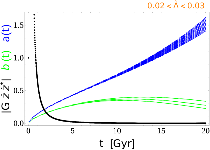
(a) The brane’s scale factor $a$ (blue), the bulk’s scale factor $b$ (green), and $\left|{G_{i\bar{j}}\dot{z}^{i}\dot{z}^{\bar{j}}}\right|$ (black) are plotted versus time for $0.02<\tilde{\Lambda}<0.03$. $a_{0}=1$, and $t_{0}=13.842~{}[\text{Gyr}]$.

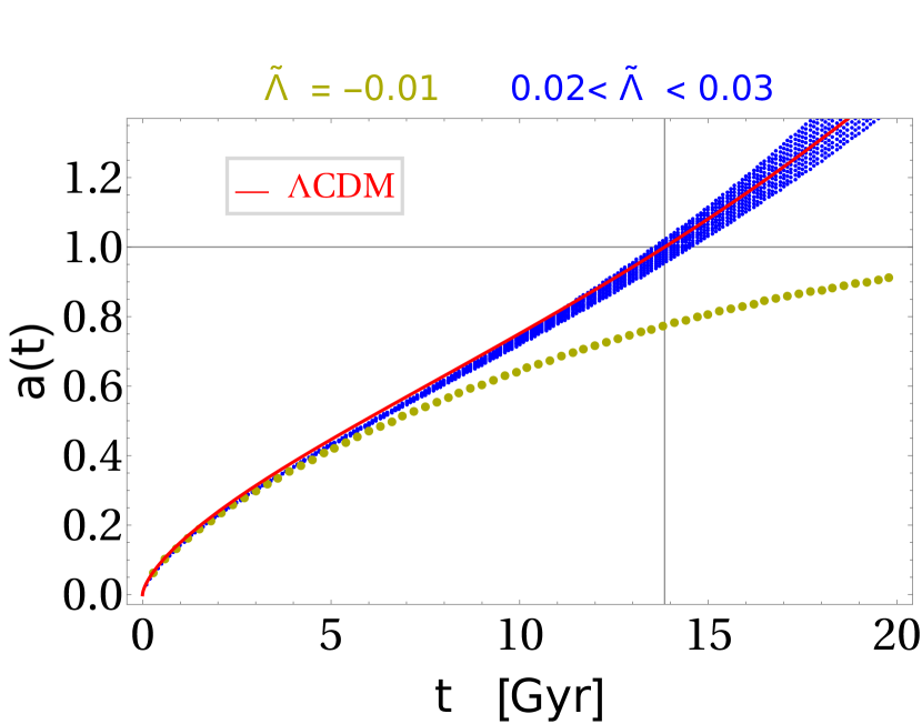
(b) The brane’s scale factor (blue) fits the scale factor of the $\Lambda$CDM model (red) for the range $0.02<\tilde{\Lambda}<0.03$. The yellow curve shows the brane’s scale factor for $\tilde{\Lambda}=-0.01$.

Figure 1:

The first and the second equations represent the Friedmann-like equations for the brane-universe, while the third equation represents the bulk. Solving those equations numerically to get the brane’s and the bulk’s scale factors $a$ and $b$, respectively, and the moduli’s flow velocity $G_{i\bar{j}}\dot{z}^{i}\dot{z}^{\bar{j}}$ [21]. We scan over a range of the bulk’s cosmological constant $0.02<\tilde{\Lambda}<0.03$. Whilst the solutions are valid for a wide range of initial conditions fine-tuning. Here we take $a[0]=b[0]\sim 0.06$ and $a^{\prime}[0]=b^{\prime}[0]\sim 0.01$. In our model, we consider the value of the dark energy density parameter $\Omega_{\Lambda}=0$, and the current matter density parameter $\Omega_{m0}\sim 0.99$, so in our model the main components of the brane-universe are only matter and radiation. In the $\Lambda$CDM model according to the recent Planck mission data based on CMB (The Cosmic Microwave Background) [22] $\Omega_{m0}=0.3111$, the current radiation density parameter $\Omega_{r0}=8.2\times 10^{-5}$, and $\Omega_{\Lambda 0}=0.6889$. The current value of the Hubble parameter is given by $H_{0}=0.0686751~{}[\text{Gyr}^{-1}]\sim 2.176\times 10^{-18}~{}[\text{sec}^{-1}]$. The age of the universe is $t_{0}=13.842~{}[\text{Gyr}]$. That amount of $\Omega_{m0}$ in the brane-universe means that the current dark matter density parameter $\Omega_{Dm0}\sim 0.94$ in the brane because the current baryonic matter density parameter in our universe is $\Omega_{Bm0}=0.0463\pm 0.0024$. That huge amount of $\Omega_{Dm0}$ in the brane may affect other cosmological observable like the baryonic acoustic oscillation or the galactic rotations curves. However, next, we will show that the cosmic evolution of the brane-universe is similar to the expansion history of our universe according to BOSS collaboration data based on the baryon acoustic oscillation (BAO) and the CMB constraints [23].

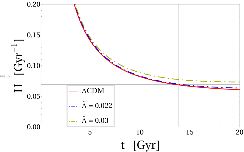
(a) The Hubble parameter of $\Lambda$CDM (red), the brane’s Hubble parameters for $\tilde{\Lambda}=0.022~{}[\text{Gyr}^{-2}]$ (blue dashed) and $\tilde{\Lambda}=0.03~{}[\text{Gyr}^{-2}]$ (yellow dashed) are plotted versus time. $H_{0}=0.0689751~{}[\text{Gyr}^{-1}]$.

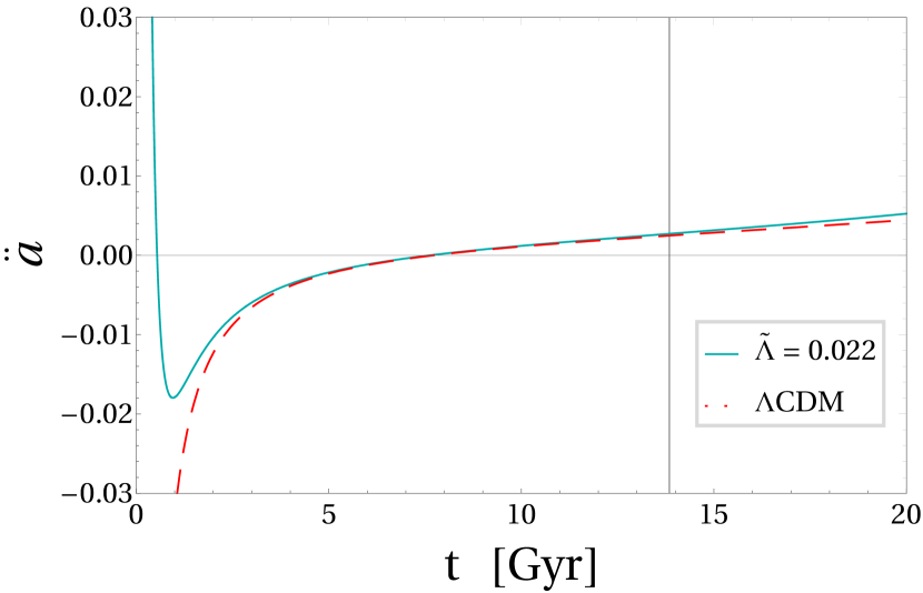
(b) The acceleration of the brane’s scale factor (blue) and the acceleration of the scale factor of $\Lambda$CDM (red dashed) are plotted versus time. Around $t=10~{}[\text{Gyr}]$ the accelerated expansion has been initiated.

Figure 2:

In Fig. (1(a)) the brane’s and the bulk’s scale factors, and the absolute value of the moduli velocity norm are plotted versus time. Through these ranges $a[t_{0}]=1$ as the scale factor of the $\Lambda$CDM model. The bulk’s scale factor varies by different values and it is inversely proportional to $\tilde{\Lambda}$. Also the correlation between $G_{i\bar{j}}\dot{z}^{i}\dot{z}^{\bar{j}}$ and $a(t)$ is clear, as the moduli are maximum $a(t)$ is minimum, and vise versa. Fig. (1(b)) shows that the scale factor of the brane (blue) fits and the $\Lambda$CDM’s scale factor (red) over the scanned parameter region, where the current value of the $\Lambda$CDM’s scale factor $a(t_{0})$ is normalized to $a_{0}=1$. While for instance, an Anti-de Sitter bulk with a negative $\tilde{\Lambda}$ leads the brane-univesre for a deceleration. Fig. (2(a)) shows that brane’s Hubble parameter (blue dashed) fits the Hubble parameter of the $\Lambda$CDM model (red) at $\tilde{\Lambda}=0.022$. The horizontal line is at $H_{0}$. In Fig. (2(b)) the acceleration of the brane’s scale factor at $\tilde{\Lambda}=0.022$ (blue) and the acceleration of the scale factor of $\Lambda$CDM (red dashed) are plotted versus time. We can see the deceleration and the acceleration eras that happened after the big bang by $(3-5)$ Gyr and $(9-10)$ Gyr, respectively, according to the BOSS’s data. Such that during the decelerated expansion the brane’s acceleration was negative ($\ddot{a}<0$), then around $10$ Gyr ($\ddot{a}>0$) till the present time $(t_{0})$. Through those epochs the brane and the $\Lambda$CDM’s accelerations coincide, while in the early times, the brane’s acceleration shows inflationary behavior ($\ddot{a}>0$) which the $\Lambda$CDM model does not explain. In the next graphs, we will show clearly the very early ages of the expansion.

IV The cosmic history

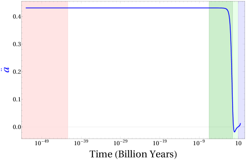
Figure 3: The acceleration of the brane’s scale factor is plotted versus time on a logarithmic scale ($\tilde{\Lambda}=0.022$.). The pink area corresponds to the inflation era, the dark green area when the CMB happens, the light green area when the deceleration expansion happened, and the light blue area corresponds to the late-time acceleration era.

In Fig. (3) the acceleration of the brane-universe is plotted versus time on a logarithmic scale. We can see that the early times are zoomed in, and the whole cosmic evolution of the universe is shown. The pink era is when the inflation started around $t\sim 10^{-53}~{}[\text{Gyr}]$ and ended on $t\sim 10^{-43}~{}[\text{Gyr}]$ where ($\ddot{a}>0$). Then the dark green era when the CMB happened, the light green era when the decelerated expansion took place, and the light blue era corresponds to the late-time acceleration expansion.

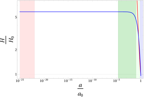
Figure 4: $H(a)/H_{0}$ for the brane-universe (blue) and the $\Lambda$CDM model (red) are plotted versus the expansion scale factor. The pink area is a high regime era where $H>>H_{0}$, which corresponds to the inflation era, and the dark green area is when the CMB happens. Then $H/H_{0}$ starts to get close to unity as the brane starts deceleration expansion through the light green area. The light blue area when the accelerated expansion started at $a\sim 0.7$ till the time beings.

In Fig. (4) the Hubble parameter $H(a)/H_{0}$ for the brane (blue) and the $\Lambda$CDM model (red) are plotted as functions in the expansion scale factor $(a/a_{0})$ on a logarithmic scale ($\tilde{\Lambda}=0.022$). The pink area corresponds to the inflation era, and the dark green area starts when the CMB happened after the big bang by $t_{CMB}=380.000$ years and $a[t_{CMB}]\sim 2.3\times 10^{-5}~{}[\text{Gyr}]$. The light green era corresponds to when the deceleration of the universe’s expansion happened, and the light blue era corresponds to when the late-time acceleration happens after $(9-10)$ billion years of the big bang till time beings. That is according to the experimental data of our universe’s expansion based on the baryon acoustic oscillation (BAO) reported by BOSS collaboration. We can see that $H(a)/H_{0}$ of the brane met that of the $\Lambda$CDM during the deceleration era. It is also shown that ($a/a_{0}$) through the inflation period where there are enough number of e-folds $N=ln(a_{e}/a_{0})$ (e stands for the end of the inflation) to solve the Horizon problem. Let us draw the attention that the values of $\tilde{\Lambda}$ are given in [$\text{Gyr}^{-2}$]. For the sake of comparison, the value of $\Lambda$ in $\Lambda$CDM is given by $\frac{8\pi G}{c^{2}}~{}\rho^{obs}_{\Lambda}~{}\sim 9.7\times 10^{-36}~{}\text{sec}^{-2}\sim 0.00969~{}\text{Gyr}^{-2}$, while for instance $\tilde{\Lambda}=0.022~{}\text{Gyr}^{-2}=5.5\times 10^{-35}~{}\text{sec}^{-2}$. Fig. (5) shows the relation of the moduli to the inflation slow-roll parameter $\epsilon=-\frac{\dot{H}}{H^{2}}$, where $\epsilon$ is plotted against the moduli’s flow velocity $|\dot{z}|^{2}\equiv\left({G_{i\bar{j}}\dot{z}^{i}\dot{z}^{\bar{j}}}\right)$ at $\tilde{\Lambda}=0.022$ (blue) and $\tilde{\Lambda}=0.03$ (green). We can see that when the moduli have larger values $\epsilon<1$ at inflation which means that $H$ is varying slowly or there is an accelerated phase of expansion. Then when $|\dot{z}|^{2}$ decrease the inflation ends, where $\epsilon>1$.

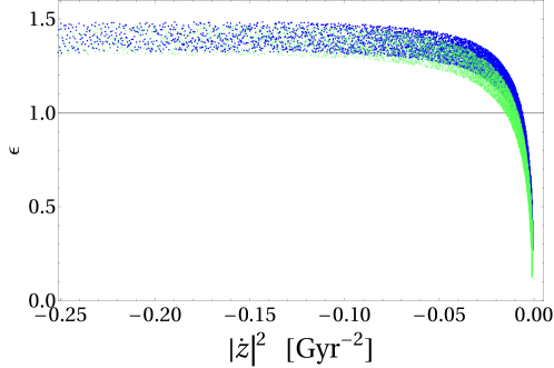
Figure 5: The slow-roll parameters are plotted against the moduli’s flow velocity $({G_{i\bar{j}}\dot{z}^{i}\dot{z}^{\bar{j}}})$ at $\tilde{\Lambda}=0.022$ (blue) and $\tilde{\Lambda}=0.03$ (green).

V Finding analytic solution

To find an analytic solution for the field equations (18), we consider the bulk has a constant size, i.e., the bulk’s scale factor is constant $(\dot{b}=0)$. The field equations simplify to:

$$3\left({\frac{{\dot{a}}}{a}}\right)^{2} = G_{i\bar{j}}\dot{z}^{i}\dot{z}^{\bar{j}}+\rho,$$

$$2\frac{{\ddot{a}}}{a}+\left({\frac{{\dot{a}}}{a}}\right)^{2} = -p-G_{i\bar{j}}\dot{z}^{i}\dot{z}^{\bar{j}},$$

$$\left[{\frac{{\ddot{a}}}{a}+\left({\frac{{\dot{a}}}{a}}\right)^{2}}\right] = \tilde{\Lambda}-G_{i\bar{j}}\dot{z}^{i}\dot{z}^{\bar{j}}.$$ (20)

Eliminating $(G_{i\bar{j}}\dot{z}^{i}\dot{z}^{\bar{j}})$ gives:

$$p = \frac{2\dot{a}^{2}}{a}+\frac{\ddot{a}}{a}+\tilde{\Lambda},$$

$$\rho = \frac{4\dot{a}^{2}}{a^{2}}+\frac{2\ddot{a}}{a}+p.$$ (21)

Solving these couple of equations gives:

$$a(t) = c_{2}\cos\left[\sqrt{\frac{3}{2}}\sqrt{p-\rho}(t+2c_{1})\right]^{1/3},$$ (22)

$$= c_{2}\cos\left[\sqrt{3}\sqrt{\tilde{\Lambda}-p}(t-c_{1})\right]^{1/3}.$$

Where $c_{1}$ and $c_{2}$ are the integration constants. That sets a constrain on the density $\rho$ and the pressure $p$ in the brane, and $\tilde{\Lambda}$ in the bulk, $3p-2\rho=\tilde{\Lambda}.$

Another thing we want to declare about that class of models with a null cosmological constant ($\Lambda=0$) [24], that they can prompt the string theory to be a theory of quantum gravity. If our universe as described in this paper has no cosmological constant, the Swampland conjectures do not apply to the string theory as a low-energy theory of our universe.

VI Conclusion

What is the origin of the late-time accelerated expansion of the universe? We find It difficult to accept that its origin is the cosmological constant in Einstein’s general relativity because in GR the cosmological constant is related to the vacuum energy density which is tremendously large compared to the observed energy density (dark energy) that is responsible for the universe’s accelerated expansion. In this paper, we introduced a new explanation for dark energy by modeling the universe as a symplectic 3-brane embedded in a five-dimensional bulk of $\mathcal{N}=2$ supergravity. The brane-universe has an early time inflation, followed by deceleration, then followed by a late-time acceleration adequate to our universe’s cosmic evolution. Although the 3-brane has a zero cosmological constant, solving the modified Friedmann’s equations shows that the fields which drive the dynamics of the brane and the bulk are the complex structure moduli of the Calabi-Yau manifold. The bulk should be a di-Sitter space with a non-vanishing cosmological constant. The results correspond to the $\Lambda$CDM model and agree with the recent experimental data presented by BOSS collaboration about our universe’s expansion history based on the baryon acoustic oscillation (BAO) combined with the CMB constraints. So our model gives an entire explanation of the whole time evolution of the universe, from inflation to the current time acceleration based on topological effects, and a fifth dimension. We would like to point out that in light of the results presented in this work, there are many other quests opened for future research, like studying the dynamics of the Calabi-Yau manifold itself and its complex structure moduli, investigating the moduli dependence on the extra fifth dimension, since here only the time dependence is considered, fully analyzing the inflationary period, what is the nature of the bulk’s cosmological constant? Is the bulk’s energy density like the energy density proposed in the $\Lambda$CDM model? Although the results agree with the BAO’s data, what are the consequences of assuming a large amount of dark energy in the brane? Finally, what are the implications of the analytic solutions of the field equations.

References

• [1] C. L. Bennett, et al “Nine-year Wilkinson Microwave anisotropy probe (WMAP) observations: Final maps and results,” The atrophysical journal supplement series, volume 208, number 2 (2013) doi:10.1088/0067-0049/208/2/20 [arXiv:1212.5225 [astro-ph]].
• [2] S. Tsujikawa, “Introductory review of cosmic inflation,” hep-ph/0304257.
• [3] S. Perlmutter, et al., “Measurements of $\Omega$ and $\Lambda$ from 42 high redshift supernovae,” Astrophys. J. 517 (1999) 565-586, arXiv:astro-ph/9812133.
• [4] A.G. Riess, et al., “Observational evidence from supernovae for an accelerating universe and a cosmological constant,” Astron. J. 116 (1998) 1009-1038, arXiv:astro-ph/9805201.
• [5] R. R. Caldwell, and M. Kamionkowski, “The physics of cosmic acceleration,” Annual Review of Nuclear and Particle Science, Vol. 59:397-429 (2009) doi:10.1146/annurev-nucl-010709- 151330.
• [6] Sean M. Carroll, et al., “The Cosmological Constant,” Ann. Rev. Astron. Astrophys. 30 (1992) 499-542.
• [7] S.E. Rugh, H. Zinkernagel, “The Quantum vacuum and the cosmological constant problem,” Stud. Hist. Philos. Sci. B 33 (2002) 663-705, arXiv:hep-th/0012253.
• [8] M. Nishimura, “Conformal supergravity from the AdS/CFT correspondence,” Nucl. Phys. B 588 (2000) 471–482, hep-th/0004179.
• [9] L. Jarv, T. Mohaupt, and F. Saueressig, “ M-theory cosmologies from singular Calabi-Yau compactifications,” JCAP 0402 (2004) 012, hep-th/0310174.
• [10] R. Maartens and K. Koyama, “Brane-World Gravity,” Living Rev. Rel. 13, 5 (2010) doi:10.12942/lrr-2010-5 [arXiv:1004.3962 [hep-th]].
• [11] A. D. Linde, “Recent progress in inflationary cosmology,” Lect. Notes Phys. 455 (1995) 363-372. Contribution to: International Workshop on the Birth of the Universe and Fundamental Physics, 363-372, LLWI 1994, 72-109, hep-th/9410082.
• [12] K. Koyama, “The cosmological constant and dark energy in braneworlds,” Gen. Rel. Grav. 40, 421 (2008), astro-ph/0706.1557.
• [13] A. C. Cadavid, A. Ceresole, R. D’Auria and S. Ferrara, “Eleven-dimensional supergravity compactified on Calabi-Yau threefolds,” Phys. Lett. B 357 (1995) 76–80, hep-th/9506144.
• [14] M. Dine, R. Kitano, A. Morisse and Y. Shirman, “Moduli decays and gravitinos,” Phys. Rev. D 73, 123518 (2006) [hep-ph/0604140].
• [15] D. Bodeker, “Moduli decay in the hot early universe,” JCAP 0606, 027 (2006) [hep- ph/0605030].
• [16] K. S. Stelle, “ BPS Branes in Supergravity,” NATO Sci. Ser. C 530 (1999) 257 [hep-th/9803116]. D. N. Kabat and A. Rajaraman, “Testing cosmological supersymmetry breaking,” Phys. Lett. B 516, 383 (2001) [hep-ph/0102309]; M. H. Emam, “Zero-branes and the symplectic hypermultiplets,” Phys. Rev. D 86, 045016 (2012) [hep-th/1208.3488].
• [17] J. P. Ostriker, Paul J. Steinhardt, “The Observational case for a low density universe with a nonzero cosmological constant, ” Nature 377 (1995) 600.
• [18] M. H. Emam, “BPS brane cosmology in N = 2 supergravity,” Class. Quant. Grav. 32, no. 18, 185014 (2015) doi:10.1088/0264-9381/32/18/185014 [arXiv:1509.01651 [hep-th]].
• [19] M. Emam, H. H. Salah, and S. Salem, “Brane-worlds and the Calabi- Yau complex structure moduli”, Class. Quant. Grav. 37, 195007 (2020) hep-th/2005.10408.
• [20] M. H. Emam, “The Many symmetries of Calabi-Yau compactifications,” Class. Quant. Grav. 27, 163001 (2010) [arXiv:1007.4847 [hep-th]].
• [21] Safinaz Salem, Moataz H. Emam, and H.H. Salah, “ The implications of $\mathcal{N}=2$ Supergravity Cosmology On the Topology of the Calabi-Yau Manifold,” [arXiv:gr-qc/2204.13776].
• [22] Planck Collaboration, Y. Akrami, et al., “Planck 2018 results. VI. Cosmological parameters,” Astron. Astrophys. 641 (2020) A6, arXiv:astro-ph/1807.06209.
• [23] BOSS Collaboration, Timothée Delubac, et al., “Baryon acoustic oscillations in the Ly$\alpha$ forest of BOSS quasars,” Astron.Astrophys. 574 (2015) A59, arXiv:astro-ph.CO/1404.1801.
• [24] L.G. Jaime, G. Arciniega, “A unified geometric description of the universe: From inflation to late-time acceleration without an inflaton nor a cosmological constant,” Phys. Lett. B 827 (2022) 136939.