Abstract

Estimation problems with constrained parameter spaces arise in various settings. In many of these problems, the observations available to the statistician can be modelled as arising from the noisy realization of the image of a random linear operator; an important special case is random design regression. We derive sharp rates of estimation for arbitrary compact elliptical parameter sets and demonstrate how they depend on the distribution of the random linear operator. Our main result is a functional that characterizes the minimax rate of estimation in terms of the noise level, the law of the random operator, and elliptical norms that define the error metric and the parameter space. This nonasymptotic result is sharp up to an explicit universal constant, and it becomes asymptotically exact as the radius of the parameter space is allowed to grow. We demonstrate the generality of the result by applying it to both parametric and nonparametric regression problems, including those involving distribution shift or dependent covariates.

1 Introduction

In this paper, we study the problem of estimating an unknown vector $\theta^{\star}$ on the basis of random linear observations corrupted by noise. More concretely, suppose that we observe a random operator $T_{\xi}$ and a random vector $y$, which are linked via the equation

$$y=T_{\xi}(\theta^{\star})+w.$$ (1)

This observation model involves two forms of randomness: the unobserved vector $w$, which is a form of additive observation noise, and the observed operator $T_{\xi}$, which is random, as indicated by its dependence on an underlying random variable $\xi$.

While relatively simple in appearance, the observation model (1) captures a broad range of statistical estimation problems.

Example 1 (Linear regression).

We begin with a simple but widely used model: linear regression. The goal is to estimate the coefficients $\theta^{\star}\in{}^{d}$ that define the best linear predictor $x\mapsto\langle x,\,\theta^{\star}\rangle$ of some real-valued response variable $Y\in\real$. In order to do so, we observe a collection of $(x_{i},y_{i})$ pairs linked via the noisy observation model

$$y_{i} =\langle x_{i},\,\theta^{\star}\rangle+w_{i}\qquad\mbox{for $i=1,\ldots,n$.}$$

If we define the concatenated vector $y=(y_{1},\ldots,y_{n})$, with an analogous definition for $w$, this is a special case of our general setup with the random linear operator $T_{\xi}:\mathbf{R}^{d}\rightarrow\mathbf{R}^{n}$ given by

$$[T_{\xi}(\theta)]_{i} =\langle x_{i},\,\theta\rangle\quad\mbox{for $i=1,\ldots,n$.}$$ (2)

Here, the random index corresponds to the covariate vectors so that $\xi=(x_{1},\dots,x_{n})$; note that we have imposed no assumptions on the dependence structure of these covariate vectors. In the classical setting, these covariates are assumed to be drawn in an i.i.d. manner; however, our general set-up is by no means limited to this classical setting. In the sequel, we consider various examples with interesting dependence structure, and our theory gives some very precise insights into the effects of such dependence.

Example 2 (Nonparametric regression).

In the preceding example, we discussed the problem of predicting a response variable $Y\in\real$ in a linear manner. Let us consider the nonparametric generalization: here our goal is to estimate the regression function $f^{\star}(x)\coloneq\operatorname*{\mathbf{E}}\ilimits@[Y\mid X=x]$, which need not be linear as a function of $x$. Given observations $\{(x_{i},y_{i})\}_{i=1}^{n}$, we can write them in the form

$$y_{i} =f^{\star}(x_{i})+w_{i},\qquad\mbox{for $i=1,\ldots,n$,}$$

where $w_{i}=y_{i}-\operatorname*{\mathbf{E}}\ilimits@[Y\mid X=x_{i}]$ are zero-mean noise variables.

Now let us suppose that $f^{\star}$ belongs to some function class $\mathcal{F}$ contained with $L^{2}(\mathcal{X})$, and show how this observation model can be understand as a special case of our setup with $\theta^{\star}\in\ell^{2}(\mathbf{N})$. Take some orthonormal basis $\{\phi_{j}\}_{j\geqslant 1}$ of $L^{2}(\mathcal{X})$. Any function in $\mathcal{F}$ can then be expanded as $f=\sum_{j\geqslant 1}\theta_{j}\phi_{j}$ for some sequence $\theta\in\ell^{2}(\mathbf{N})$. Letting $\xi=(x_{1},\ldots,x_{n})$, we can define the operator $T_{\xi}:\ell^{2}(\mathbf{N})\rightarrow\mathbf{R}^{n}$ via

$$\theta\mapsto[T_{\xi}(\theta)]_{i} \coloneq\sum_{j=1}^{\infty}\theta_{j}\phi_{j}(x_{i})\quad\mbox{for $i=1,\ldots,n$},$$

so that this problem can be written in the form of our general model (1). Observe that the randomness in the observation operator $T_{\xi}$ arises via the randomness in sampling the covariates $\{x_{i}\}_{i=1}^{n}$.

Example 3 (Tomographic reconstruction).

The problem of tomographic reconstruction refers to the problem of recovering an image, modeled as a real-valued function $f^{\star}$ on some compact domain $\mathcal{X}\subset{}^{2}$, based on noisy integral measurements. Formally, we observe responses of the form

$$y_{i} =\int_{\mathcal{X}}h(x_{i},u)f^{\star}(u)\,\mathrm{d}u+w_{i}\qquad\mbox{for $i=1,\ldots,n$,}$$

where $h:{}^{2}\times{}^{2}\rightarrow\real$ is a known window function. If we again view $f^{\star}$ as belonging to some function class $\mathcal{F}$ within $L^{2}(\mathcal{X})$, then we can write this model in our general form with

$$[T_{\xi}(v)]_{i} =\sum_{j\geqslant 1}v_{j}\Big{[}\int_{\mathcal{X}}h(x_{i},u)\phi_{j}(u)\,\mathrm{d}u\Big{]},\quad\mbox{and $\xi=(x_{1},\ldots,x_{n})$.}$$

Here we have followed the same conversion as in Example 2, in particular re-expressing $f^{\star}$ in terms of its generalized Fourier coefficients with respect to an orthonormal family $\{\phi_{j}\}_{j\geqslant 1}$.

Example 4 (Error-in-variables).

Consider the Berkson variant [6, 14] of the error-in-variables problem in nonparametric regression. In this problem, an observed covariate $x$—instead of being associated with a noisy observation of $f^{\star}(x)$—is associated with a noisy observation of the “jittered” evaluation $f^{\star}(x+u)$, where $u\in\mathbf{R}$ is the random jitter. Formally, we observe $n$ pairs $(x_{i},y_{i})$ of the form

$$y_{i} =f^{\star}(x_{i}+u_{i})+\varepsilon_{i}\qquad\mbox{for $i=1,\ldots,n$,}$$

where the unobserved random jitter $u_{i}$ is drawn independently of the pair $(x_{i},\varepsilon_{i})$. We can re-write these observations as a special case of our general model with $\xi=(x_{1},\ldots,x_{n})$, and

$$[T_{\xi}(f)]_{i}\coloneq\operatorname*{\mathbf{E}}\ilimits@_{u}\big{[}f(x_{i}+u)\big{]},\quad\mbox{and}\quad w_{i}\coloneq\varepsilon_{i}+\Big{\{}f(x_{i}+u_{i})-\operatorname*{\mathbf{E}}\ilimits@_{u}\big{[}f(x_{i}+u)\big{]}\Big{\}}\quad\mbox{for $i=1,\ldots,n$.}$$

Note that the new noise variables $w_{i}$ are again zero-mean, and our assumption that $T_{\xi}$ is observed means that the distribution of the jitter $u$ is known.

These examples (and others, as discussed below in Section 1.2) motivate our study of the operator model (1). As we discuss in further detail later, a key advantage of writing the observation model in this form is that it will allow us to separate three key components of the difficulty of the problem: (i) the distribution of the random operator $T_{\xi}$, as expressed via the distribution of $\xi$, (ii) the distribution of the noise variable $w\coloneq y-T_{\xi}\theta^{\star}$, and (iii) the constraints on the unknown parameter $\theta^{\star}$.

1.1 Problem formulation, notation, and assumptions

With these motivating examples in mind, we now turn to a more precise mathematical formulation of the estimation problem introduced above.

1.1.1 Assumptions on the random variables $(\xi,w)$

Let us start by discussing properties of the random operator $T_{\xi}$. In the examples previously introduced, the domain of the observation operator $T_{\xi}$ was either a subset of $\mathbf{R}^{d}$, or more generally, a subset of the sequence space $\ell^{2}(\mathbf{N})$. The bulk of our analysis focuses on the finite-dimensional setting —i.e., with domain $\mathbf{R}^{d}$—so that $T_{\xi}$ can be identified with a random matrix $\mathbf{R}^{n\times d}$, for some pair $(n,d)$ of positive but finite integers. However, as we highlight in Section 3.2, simple approximation arguments can be used to leverage our finite-dimensional results to determine minimax rates of convergence for estimating an element $\theta^{\star}$ of the infinite-dimensional sequence space $\ell^{2}(\mathbf{N})$.

In terms of the probabilistic structure of $T_{\xi}$, we assume the random element $\xi$ lies in the measurable space $(\Xi,\mathcal{E})$, and is drawn from a probability measure $\mathbb{P}$ on the same space. Throughout we take $\mathcal{E}$ to be large enough such that linear functionals of $T_{\xi}$ are measurable.

As for the noise vector $w\in\mathbf{R}^{n}$, we assume it is drawn—conditionally on $\xi$—from a noise distribution with conditional mean zero, and bounded conditional covariance. Formally, we assume that $w\sim\nu(\cdot\mid\xi)$ where $\nu$ is a Borel regular conditional probability on $\mathbf{R}^{n}$ that satisfies the following two conditions:

1. For $\mathbb{P}$-almost every $\xi\in\Xi$, we have $\int w\,\nu(\mathrm{d}w\mid\xi)=0$; and

2. For $\mathbb{P}$-almost every $\xi\in\Xi$, we have

   $$\int(u^{\mathsf{T}}w)^{2}\,\nu(\mathrm{d}w\mid\xi)\leqslant u^{\mathsf{T}}\Sigma_{w}u,\qquad\mbox{for any fixed}~{}u\in\mathbf{R}^{n}.$$

We write that the measure $\nu$ lies in the set $\mathcal{P}(\Sigma_{w})$ when these two conditions are satisfied.

In words, Assumption (N1) requires that $w$ is conditionally centered, and Assumption (N2) assumes that the conditional covariance of $w$ is almost surely upper bounded in the semidefinite ordering by $\Sigma_{w}$. Let $\mathbb{P}\times\nu$ denote the distribution of the tuple $(\xi,w)$; in explicit terms, writing $(\xi,w)\sim\mathbb{P}\times\nu$ means that $\xi\sim\mathbb{P}$ and $w\mid\xi\sim\nu(\cdot\mid\xi)$. Having specified the joint law of $(\xi,w)$, the random variable $y$ then satisfies the stated observation model (1).

1.1.2 Decision-theoretic formulation

In this paper, our goal to estimate $\theta^{\star}$ to the best possible accuracy as measured by a fixed quadratic form. To make this rigorous, we introduce two symmetric positive definite matrices ${K_{e}}$ and ${K_{c}}$, which induce (respectively) the squared norms

$$\|\theta\|_{{K_{e}}}^{2}\coloneq\langle\theta,{K_{e}}\theta\rangle\quad\mbox{and}\quad\|\theta\|_{{K_{c}}^{-1}}^{2}\coloneq\langle\theta,{K_{c}}^{\!-1}\theta\rangle,$$

defined for any $\theta\in\mathbf{R}^{d}$. We seek estimates $\widehat{\theta}$ of $\theta^{\star}$ that have low squared estimation error $\lVert\widehat{\theta}-\theta^{\star}\rVert_{{K_{e}}}^{2}$, as defined by the matrix ${K_{e}}$. In parallel, we assume that underlying parameter is bounded in the constraint norm, so that it lies in the ellipse

$$\Theta(\varrho,{K_{c}})\coloneq\Big{\{}\,\theta\in\mathbf{R}^{d}:\lVert\theta\rVert_{{K_{c}}^{-1}}\leqslant\varrho\,\Big{\}}$$

with radius $R$, as defined by the matrix ${K_{c}}$.

With this notation in hand, the central object of study in this paper is the minimax risk

$$\mathfrak{M}(T,\mathbb{P},\Sigma_{w},\varrho,{K_{e}},{K_{c}}) \coloneq\inf_{\widehat{\theta}}\sup_{\begin{subarray}{c}\theta^{\star}\in\Theta(\varrho,{K_{c}})\\ \nu\in\mathcal{P}(\Sigma_{w})\end{subarray}}\operatorname*{\mathbf{E}}\ilimits@_{(\xi,w)\sim\mathbb{P}\times\nu}\Big{[}\lVert\widehat{\theta}-\theta^{\star}\rVert^{2}_{{K_{e}}}\Big{]},$$ (3)

where the infimum ranges over all measurable functions $\widehat{\theta}\equiv\widehat{\theta}(T_{\xi},y)$ that map the observed pair $(T_{\xi},y)$ to $\mathbf{R}^{d}$.

1.2 Examples of choices of sampling laws, constraints and error norms

As discussed previously, our general theory accommodates various forms of the random linear operators $T_{\xi}$. As might one expect, the sampling law $\mathbb{P}$ for $\xi$ changes the statistical structure of the observations, and so influences the quality of the best possible estimates. Moreover, the interaction between $\mathbb{P}$ and the geometry of the error norm, as defined by the matrix ${K_{e}}$, plays an important role. Finally, both of these factors interact with the geometry of the constraint set, as determined by the matrix ${K_{c}}$.

Below we discuss some examples of these types of interactions. To be clear, each of these statistical settings have been considered separately in the literature previously; one benefit of our approach is that it provides a unifying framework that includes each of these problems as special cases.

Example 5 (Covariate shift in linear regression).

Recall the set-up for linear regression, as introduced in Example 1. In practice, the source distribution from which the covariates $x$ are sampled when constructing an estimate of $\theta^{\star}$ need not be the same as the target distribution of covariates on which the predictor is to be deployed. This phenomenon—a discrepancy between the source and target distributions—is known as covariate shift. It is now known to arise in a wide variety of applications (e.g., see the papers [45, 40] and references therein for more details).

As one concrete example, in healthcare applications, the covariate vector $x\in\mathbf{R}^{d}$ might correspond to various diagnostic measures run on a given patient, and the response $y\in\mathbf{R}$ could correspond to some outcome variable (e.g., blood pressure). Clinicians might use one population of patients to develop a predictive model relating the diagnostic measures $x$ to the outcome $y$, but then be interested in making predictions for a related but distinct population of patients.

In our setting, suppose that we use the linear model $\theta\mapsto\widehat{y}\coloneq\langle\theta,\,x\rangle$ to make predictions over a collection of covariates with distribution $Q$. A simple computation shows that the mean-squared prediction error, averaging over both the noise $w$ and random covariates $x$, takes the form

$$\operatorname*{\mathbf{E}}\ilimits@\big{[}(\widehat{y}-y)^{2}\big{]} =\underbrace{(\theta-\theta^{\star})^{\mathsf{T}}\Sigma_{Q}(\theta-\theta^{\star})}_{\eqcolon\,L_{Q}(\widehat{\theta},\theta^{\star})}+c,\qquad\mbox{where}\quad\Sigma_{Q}\coloneq\operatorname*{\mathbf{E}}\ilimits@_{Q}[x\otimes x],$$

and $c$ is a constant independent of the pair $(\theta,\theta^{\star})$. Thus, the excess prediction error over the new population $Q$ corresponds to taking ${K_{e}}=\Sigma_{Q}$ in our general set-up. Similarly, if one wanted to assess parameter error, then studying the minimax risk with the choice ${K_{e}}=I_{d}$ would be reasonable. Finally, the error in the original population (denoted $P$) can be assessed with the choice ${K_{e}}=\Sigma_{P}\coloneq\operatorname*{\mathbf{E}}\ilimits@_{P}[x\otimes x]$.

Among the claims in the paper of Mourtada [53] is the following elegant result: when no constraints are imposed on $\theta^{\star}$, the minimax risk in the squared metric $L_{Q}(\widehat{\theta},\theta^{\star})=\|\widehat{\theta}-\theta^{\star}\|_{\Sigma_{Q}}^{2}$ is equal to

$$\inf_{\widehat{\theta}}\sup_{\theta^{\star}\in\mathbf{R}^{d}}\operatorname*{\mathbf{E}}\ilimits@\Big{[}L_{Q}(\widehat{\theta},\theta^{\star})\Big{]}=\frac{\sigma^{2}}{n}\operatorname*{\mathbf{E}}\ilimits@[\operatorname{\bf Tr}(\Sigma_{n}^{-1}\Sigma_{Q})],$$ (4)

where $\Sigma_{n}$ denotes the sample covariance matrix $(1/n)\sum_{i=1}^{n}x_{i}\otimes x_{i}$, and the expectation is over $x_{1},\dots,x_{n}\stackrel{{\scriptstyle\rm IID}}{{\sim}}P$. Thus, the fundamental rate of estimation depends on the distribution of the sample covariance matrix, the noise level, and the target distribution $Q$.

In this paper, we derive related but more general results that allow for many other choices of the error metric and, perhaps more importantly, permit the statistician to incorporate constraints on the parameter $\theta^{\star}$. We demonstrate in Section 3.1.3 that these more general results allow us to recover the known relation (23) via a simple limiting argument where the constraint radius tends to infinity.

Example 6 (Nonparametric regression with non-uniform sampling).

Consider observing covariate-target pairs $\{(x_{i},y_{i})\}_{i=1}^{n}$ where $y_{i}$ is modeled as being a noisy realization of a conditional mean function; i.e., we have $y_{i}=f^{\star}(x_{i})+w_{i}$ where $f^{\star}(x)=\operatorname*{\mathbf{E}}\ilimits@[Y\mid X=x]$, analogously to Example 2. When $f^{\star}$ is appropriately smooth and the covariates are drawn from a uniform distribution over some compact domain, this problem has been intensively studied, and the minimax risks are well-understood. However, when the sampling of the covariates $x_{i}$ is non-uniform, the possible rates of estimation can deteriorate drastically—see for instance the papers [23, 25, 24, 26, 32, 2].

Using tools from the theory of reproducing kernel Hilbert spaces (RKHSs), one can formulate this problem as an infinite-dimensional counterpart to our model (1), where the constraint parameters $(\varrho,{K_{c}})$ are determined by the Hilbert radius and the eigenvalues of the integral operator associated with the kernel. Although formally our minimax risk is defined for finite dimensional problems, via limiting arguments, it is straightforward to obtain consequences for the infinite-dimensional problem of the type discussed here, which discuss in Section 3.2.

Example 7 (Covariate shift in nonparametric regression).

Combining the scenarios in Examples 5 and 6, now consider the problem of covariate shift in a nonparametric setting. We observe samples $(x_{i},y_{i})$ where the covariates have been drawn according to some law $P$, and our goal is to construct a predictor with low risk in the squared norm defined by some other covariate law $Q$.

In our study of this setting, the constraint set is determined by the underlying function class in a manner analogous to Example 6, and the error metric is determined by the new distribution of covariates on which the estimates must be deployed, analogously to Example 5. Some recent work has studied general conditions on the pair $(P,Q)$ and the corresponding optimal rates of estimation [41, 27, 56, 47, 59, 67, 60, 28]. Among the consequences of our work are more refined results that are instance-dependent, in the sense that we characterize optimality for fixed pairs $(P,Q)$, as opposed to optimality over broad classes of $(P,Q)$ pairs. See Section 3.2.3 for a detailed discussion of these refined results.

The examples above share the common feature of being problems where estimating a conditional mean function is able to be formulated within the observation model (1). Additionally, in these examples, the fundamental hardness of the problem depends on both the structure of this function (modelled via assumptions on $\theta^{\star}$) as well as the distribution of the covariates. The goal of this paper is to build a general theory for these types of observation models, which elucidates how both the structure of $\theta^{\star}$ as well as the covariate law $\mathbb{P}$ determine the minimax rate of estimation in finite samples. In Section 3, we give concrete consequences of our general results for these types of problems.

1.3 Connections and relations to prior work

Let us discuss in more detail some connections and relations between our problem formulation and results, and various branches of the statistics literature.

Connections to random design regression

As shown by the examples discussed so far, our general set-up includes, among other problems, many variants of random design regression. This is a classical problem in statistics, with a large literature; see the sources [33, 65, 35] and references therein for an overview. The recent paper [53] also studies the analogous problem studied here when the vector $\theta^{\star}$ is allowed to be arbitrary; the only assumption made is that $\theta^{\star}\in\mathbf{R}^{d}$. In this case, it is possible to use tools from Bayesian decision theory to exhibit the minimax optimality of the ordinary least squares (OLS) estimator [53, Theorem 1]. In Section 3.1.3, we demonstrate how to obtain this result as a corollary of our more general results. Note that in applications, such as those given by the preceding examples, it is important that there is a constraint on $\theta^{\star}$. For instance, in a nonparametric regression problem, the parameter $\theta^{\star}$ denotes the coefficients of a series expansion corresponding to a conditional mean function $f^{\star}(x)=\operatorname*{\mathbf{E}}\ilimits@[Y\mid X=x]$ in an appropriate orthonormal family of functions. In this case, one can obtain consistent estimators of $f^{\star}$ only if $\theta^{\star}$ lies in a compact set.

Random design and Bayesian priors

When the the norm of the vector $\theta^{\star}$ is constrained, there are relatively few minimax results in the random design setting. On the other hand, a related Bayesian setting has been studied. In this line of work, the definition of the minimax risk is altered so that the “worst-case” supremum over $\theta^{\star}$ in the constraint set is replaced with a suitable “average”—namely the expectation over $\theta^{\star}$ drawn according to a prior distribution over the constraint set.

In addition to the clear differences in the formulation, this line of work exhibits two main qualitative differences from our paper. First, these Bayesian results have primarily been established in the proportional asymptotics framework, in the ratio $d/n$ is assumed to converge towards some aspect ratio $\gamma>0$ as both $(d,n)$ diverge to infinity. Secondly, by selecting “nice priors”, it is possible to leverage certain properties—for instance, equivariance to some group action—that can hold for both the prior and covariate law. On the other hand, our setting is somewhat more challenging in that we make no a priori assumptions about the covariate law and its relationship to the constraint set.

In more detail, when the covariates are drawn from a multivariate Gaussian, for certain constraint sets, it is possible to find a prior such that the minimax and Bayesian risks coincide. As one example, Dicker [17] studies the asymptotic minimax risk when the ratio $d/n$ is allowed to grow, and by using equivariance arguments, he obtains asymptotically minimax procedure. Proposition 3(b) in his paper gives a prior for which the minimax and Bayesian risks coincide. The thesis [52, Corollary 8.2] provides a matching asymptotic lower bound. The relation between Bayes and minimax risks in this line of work cannot be expected in general, as the arguments repose critically on the rotation invariance of the standard multivariate Gaussian. Moreover, this and other classical work on random design regression using Gaussian covariates typically hinges on special, closed-form formulae for quantities related to the distribution of the sample covariance matrix (see, e.g., the papers [62, 12, 1]).

Fixed design results

Although we focus on minimax estimation of the unknown parameter $\theta^{\star}$ in the random design setting, we note that the related fixed design setting is well studied. In fact, in classical work, Donoho studied a very similar operator-based observation model to the one considered here; a key difference is that in that work, the focus is on estimating a (scalar-valued) functional of $\theta^{\star}$ [18].

By sufficiency arguments, our problem, when instantiated in the setting of fixed design with Gaussian noise, is equivalent to mean estimation on an elliptical parameter set. It is therefore related to classical work on sharp asymptotic minimax estimation in the Gaussian sequence model [57, 31, 20, 19, 5, 29, 30]; see also the monograph [38] for a pedagogical overview of this topic. These works extend the classical line of work on estimating a constrained (possibly multivariate) Gaussian mean [15, 9, 50, 7, 48]. We refer the reader to references [49, 22], which contain a more thorough overview of prior work on minimax estimation of a parameter when a notion of ‘signal to noise ratio’ is fixed. Of course, applying an optimal fixed design estimator cannot be expected to yield an optimal random design estimator in general. This is because in the fixed design formulation, the worst-case $\theta^{\star}$ could adapt to a single design matrix, whereas in the random design formulation, the worst-case $\theta^{\star}$ must adapt to the random ensemble of design matrices induced by sampling $n$ samples in an IID fashion from a fixed covariate law.

2 Main results

We now turn to the presentation of our main results, which are upper and lower bounds on the minimax rate of estimation as defined in display (3), matching up to a constant pre-factor. These bounds are presented in Section 2.1.

2.1 General upper and lower bounds

Our general upper bounds are stated as the following functional of the distribution of the operator $T_{\xi}$; the noise covariance $\Sigma_{w}$; the constraint norm, as determined by the pair $(\varrho,{K_{c}})$; and the estimation norm, as defined by the operator ${K_{e}}$,

$$\Phi(T,\mathbb{P},\Sigma_{w},\varrho,{K_{e}},{K_{c}})\\ \coloneq\sup_{\Omega}\Big{\{}\,\operatorname*{\mathbf{E}}\ilimits@\operatorname{\bf Tr}\Big{(}{K_{e}}^{\!\!1/2}(\Omega^{-1}+T_{\xi}^{\mathsf{T}}\Sigma_{w}^{-1}T_{\xi})^{-1}{K_{e}}^{\!\!1/2}\Big{)}:\Omega\succ 0,~{}\operatorname{\bf Tr}({K_{c}}^{\!-1/2}\Omega{K_{c}}^{\!-1/2})\leqslant\varrho^{2}\,\Big{\}}.$$ (5)

Our first main result is a general upper bound.

Theorem 1 (General minimax upper bound).

The minimax risk is upper bounded as

$$\mathfrak{M}(T,\mathbb{P},\Sigma_{w},\varrho,{K_{e}},{K_{c}})\leqslant\Phi(T,\mathbb{P},\Sigma_{w},\varrho,{K_{e}},{K_{c}}).$$ (6)

See Section 4.1 for the proof.

Our second result is a complementary lower bound.

Theorem 2 (Lower bound).

The minimax risk is lower bounded as

$$\mathfrak{M}(T,\mathbb{P},\Sigma_{w},\varrho,{K_{e}},{K_{c}})\geqslant\,\Phi(T,\mathbb{P},\Sigma_{w},\tfrac{\varrho}{2},{K_{e}},{K_{c}})\geqslant\frac{1}{4}\,\Phi(T,\mathbb{P},\Sigma_{w},\varrho,{K_{e}},{K_{c}}).$$ (7)

See Section 4.2 for the proof.

Note that the functional on the righthand side of the display (7) above matches the quantity appearing in our minimax upper bound (6). Thus, in a nonasymptotic fashion, we have determined the minimax risk for this problem up the prefactor $1/4$.

Sharper lower bound constants

The constant appearing in the lower bound (7) can typically be substantially sharpened. To describe how this can be done via our results, fix a scalar $\tau\in(0,1]$ and a symmetric positive definite matrix $\Omega$, and let $Z\in\mathbf{R}^{d}$ be vector of IID standard Gaussians. Define the scalar

$$c\coloneq\tau^{2}(1-\operatorname*{\mathbf{P}}\ilimits@\{\tau^{2}\sum_{i=1}^{d}\lambda_{i}Z^{2}_{i}>1\}),$$

where $\{\lambda_{i}\}_{i=1}^{d}$ are the the eigenvalues of the matrix $(1/\varrho^{2}){K_{e}}^{1/2}\Omega{K_{e}}^{1/2}$. Then, we are able to establish the following minimax lower bound,

$$\mathfrak{M}(T,\mathbb{P},\Sigma_{w},\varrho,{K_{e}},{K_{c}})\geqslant\operatorname*{\mathbf{E}}\ilimits@\operatorname{\bf Tr}\Big{(}{K_{e}}^{\!\!1/2}(\frac{1}{c}\Omega^{-1}+T_{\xi}^{\mathsf{T}}\Sigma_{w}^{-1}T_{\xi})^{-1}{K_{e}}^{\!\!1/2}\Big{)},$$ (8)

provided that the parameter $\tau\in(0,1]$ and the symmetric positive definite matrix $\Omega$ is such that $\operatorname{\bf Tr}({K_{c}}^{\!-1/2}\Omega{K_{c}}^{\!-1/2})=\varrho^{2}$.

With appropriate choices of the pair $(\tau,\Omega)$, the lower bound (8) can lead to pre-factors that are much closer to $1$, and in some cases, converge to one under various scalings. In Section 3.1.1, we give one illustration of how the family of bounds (8) can be exploited to obtain an improvement of this type.

Form of an optimal procedure

Inspecting the proof of Theorem 1—specifically, as a consequence of Proposition 3—if the supremum on the righthand side of (5) is attained at the matrix $\Omega_{\star}$, then the following estimator, in view of the lower bound (7), is near minimax-optimal,

$$\widehat{\theta}(T_{\xi},y)\coloneq\big{(}\Omega_{\star}^{-1}+T_{\xi}^{\mathsf{T}}\Sigma_{w}^{-1}T_{\xi}\big{)}^{-1}T_{\xi}^{\mathsf{T}}\Sigma_{w}^{-1}y.$$ (9)

It is perhaps instructive to write this estimator in its “ridge” formulation

$$\widehat{\theta}(T_{\xi},y)=\mathop{\rm arg\,min}_{\vartheta\in\mathbf{R}^{d}}\Big{\{}\,\|y-T_{\xi}\vartheta\|_{\Sigma_{w}^{-1}}^{2}+\|\vartheta\|_{\Omega_{\star}^{-1}}^{2}\,\Big{\}}.$$

In the language of Bayesian statistics, our order-optimal procedure is a maximum a posteriori (MAP) estimate for $\theta^{\star}$ when $y\sim\mathsf{N}\left(T_{\xi}\theta^{\star},\Sigma_{w}\right)$ and the parameter follows the prior distribution $\theta^{\star}\sim\mathsf{N}\left(0,\Omega_{\star}\right)$. The optimal prior is identified via the choice of $\Omega_{\star}$ which is determined by the functional appearing in Theorems 1 and 2. If the supremum in (5) is not attained, then by selecting a sequence of matrices $\Omega_{k}$ that approach the maximal value of the functional, one can similarly argue there exists a sequence of estimators that approach the order-optimal minimax risk.

2.2 Independent and identically distributed regression models

An important application of our general result is for independent and identically distributed (IID) regression models of the form

$$y_{i}=\langle\theta^{\star},\psi(x_{i})\rangle+\sigma z_{i},\quad\mbox{for}~{}i=1,\ldots,n.$$ (10)

Above, we assume that $x_{i}$ are independent and identical draws from a fixed covariate distribution $P$, on some measurable space $\mathcal{X}$, and that $\psi\colon\mathcal{X}\to\mathbf{R}^{d}$. The covariates $\{x_{i}\}_{i=1}^{n}$ are independent and the conditional distribution of $z\mid x$ is an element of $\mathcal{P}(I_{n})$. The parameter $\sigma>0$ indicates the noise level; it is an upper bound on the conditional standard deviation of $y_{i}-\langle\theta^{\star},\psi(x_{i})\rangle$.

For the model described above, the following minimax risk of estimation provides the best achievable performance of any estimator, when $\theta^{\star}$ lies in a compact ellipse and the error is measured in the quadratic norm

$$\mathfrak{M}^{\rm IID}_{n}\Big{(}\psi,P,\varrho,\sigma^{2},{K_{c}},{K_{e}}\Big{)}\coloneq\inf_{\widehat{\theta}}\sup_{\begin{subarray}{c}\theta^{\star}\in\Theta(\varrho,{K_{c}})\\ \nu\in\mathcal{P}(\sigma^{2}I_{n})\end{subarray}}\operatorname*{\mathbf{E}}\ilimits@\Big{[}\big{\lVert}\widehat{\theta}(y_{1}^{n},x_{1}^{n})-\theta^{\star}\big{\rVert}_{{K_{e}}}^{2}\Big{]}.$$ (11)

Note that this problem can be formulated as an instance of our general operator formulation (1) where we take $y=(y_{1},\dots,y_{n})$, $w=\sigma(z_{1},\dots,z_{n})$, and $\xi=(x_{1},\dots,x_{n})$, so that $\mathbb{P}=P^{n}$. The operator $T_{\xi}$ is given by the $n\times d$-matrix with rows $\psi(x_{i})^{\mathsf{T}}$. In this context the following random matrix, which is a rescaling of the operator $T_{\xi}^{\mathsf{T}}T_{\xi}$, plays an important role:

$$\Sigma_{n}\coloneq\frac{1}{n}\sum_{i=1}^{n}\psi(x_{i})\otimes\psi(x_{i}).$$ (12)

In order to state the consequence of our more general results for this problem, let us introduce a functional. We denote it by $d_{n}$ to indicate that it is essentially an “effective statistical dimension” for this problem,

$$\leavevmode\resizebox{427.47876pt}{}{ $d_{n}(\psi,P,\varrho,\sigma^{2},{K_{e}},{K_{c}})\coloneq\sup_{\Omega}\!\Big{\{}\operatorname{\bf Tr}\operatorname*{\mathbf{E}}\ilimits@_{P^{n}}\!\big{[}{K_{e}}^{\!\!1/2}(\Sigma_{n}+\Omega^{-1})^{-1}{K_{e}}^{\!\!1/2}\big{]}:\Omega\succ 0,\operatorname{\bf Tr}({K_{c}}^{\!\!-1/2}\Omega{K_{c}}^{\!\!-1/2})\leqslant\frac{n\varrho^{2}}{\sigma^{2}}\Big{\}}$ }.$$ (13)

Then an immediate corollary to Theorems 1 and 2 is the following pair of inequalities for the IID minimax risk.

Corollary 1.

Under the IID regression model (10), the minimax rate of estimation as defined in equation (11) satisfies the following inequalities,

$$\frac{1}{4}\,\frac{\sigma^{2}}{n}d_{n}(\psi,P,\varrho,\sigma^{2},{K_{e}},{K_{c}})\leqslant\frac{\sigma^{2}}{n}d_{n}(\psi,P,\tfrac{\varrho}{2},\sigma^{2},{K_{e}},{K_{c}})\\ \leqslant\mathfrak{M}^{\rm IID}_{n}\Big{(}\psi,P,\varrho,\sigma^{2},{K_{e}},{K_{c}}\Big{)}\leqslant\frac{\sigma^{2}}{n}d_{n}(\psi,P,\varrho,\sigma^{2},{K_{e}},{K_{c}}).$$ (14)

So as to lighten notation, in the sequel, when the feature map $\psi$ is the identity mapping $\psi(x)=x$, we drop the parameter $\psi$ from the functional $d_{n}$ and the minimax rate $\mathfrak{M}^{\rm IID}_{n}$.

2.3 Some properties of the functional appearing in Theorems 1 and 2

As indicated by Theorem 1 and the subsequent discussion, the extremal quantity

$$\sup_{\Omega}\Big{\{}\,\operatorname*{\mathbf{E}}\ilimits@\operatorname{\bf Tr}\Big{(}{K_{e}}^{\!\!1/2}(\Omega^{-1}+T_{\xi}^{\mathsf{T}}\Sigma_{w}^{-1}T_{\xi})^{-1}{K_{e}}^{\!\!1/2}\Big{)}:\Omega\succ 0,~{}\operatorname{\bf Tr}({K_{c}}^{\!-1/2}\Omega{K_{c}}^{\!-1/2})\leqslant\varrho^{2}\,\Big{\}}$$ (15)

is fundamental in that it determines our minimax risk; moreover when the supremum is attained, the maximizer defines an order-optimal estimation procedure (see equation (9)). Conveniently, it turns out that the maximization problem implied by the display (15) is concave.

Proposition 1 (Concavity of functional).

The optimization problem

maximize $$f(\Omega)\coloneq\operatorname{\bf Tr}\operatorname*{\mathbf{E}}\ilimits@\big{[}{K_{e}}^{\!1/2}\big{(}\Omega^{-1}+T_{\xi}^{\mathsf{T}}\Sigma_{w}^{-1}T_{\xi}\big{)}^{-1}{K_{e}}^{\!1/2}\big{]}$$ (16)

subject to $$\Omega\succ 0,\quad\operatorname{\bf Tr}({K_{c}}^{\!-1/2}\Omega{K_{c}}^{\!-1/2})\leqslant\varrho^{2},$$

is equivalent to a convex program, with variable $\Omega$. Formally, the constraint set above is convex, and function $f$ is concave over this set.

See Appendix A.1 for the proof.

Note that this claim implies that, provided oracle access to the objective function $f$ appearing above, one can in principle obtain a maximizer in a computationally tractable manner, by leveraging algorithms for convex optimization [11].

The functional (15) depends on the distribution of $T_{\xi}^{\mathsf{T}}\Sigma_{w}^{-1}T_{\xi}$. In general, Jensen’s inequality along with the convexity of the trace of the inverse of positive matrices [8, Exercise 1.5.1] implies that it is always lower bounded by

$$\sup_{\Omega}\Big{\{}\,\operatorname{\bf Tr}\Big{(}{K_{e}}^{\!\!1/2}(\Omega^{-1}+\operatorname*{\mathbf{E}}\ilimits@T_{\xi}^{\mathsf{T}}\Sigma_{w}^{-1}T_{\xi})^{-1}{K_{e}}^{\!\!1/2}\Big{)}:\Omega\succ 0,~{}\operatorname{\bf Tr}({K_{c}}^{\!-1/2}\Omega{K_{c}}^{\!-1/2})\leqslant\varrho^{2}\,\Big{\}}$$ (17)

Comparing displays (15) and (17), we have simply moved the expectation over $\xi$ into the inverse. For certain IID regression models, as described in Section 2.2, we can give a complementary upper bound. To state our result, we define

$$\leavevmode\resizebox{427.47876pt}{}{$\overline{d}_{n}(P,\varrho,\sigma^{2},{K_{e}},{K_{c}})\coloneq\sup_{\Omega}\!\Big{\{}\operatorname{\bf Tr}\big{(}{K_{e}}^{\!\!1/2}(\operatorname*{\mathbf{E}}\ilimits@_{P^{n}}\Sigma_{n}+\Omega^{-1})^{-1}{K_{e}}^{\!\!1/2}\big{)}:\Omega\succ 0,\operatorname{\bf Tr}({K_{c}}^{\!\!-1/2}\Omega{K_{c}}^{\!\!-1/2})\leqslant\frac{n\varrho^{2}}{\sigma^{2}}\Big{\}}$ }.$$ (18)

Note that this quantity only depends on the distribution $P^{n}$ through the matrix $\operatorname*{\mathbf{E}}\ilimits@_{P^{n}}\Sigma_{n}$.

Proposition 2 (Comparison of $d_{n}$ to $\overline{d}_{n}$).

Suppose that $\Sigma_{P}\coloneq\operatorname*{\mathbf{E}}\ilimits@_{P}[\psi(x)\otimes\psi(x)]$ is nonsingular. Define $\kappa$ to be the $P$-essential supremum of $x\mapsto\|{K_{c}}^{1/2}\psi(x)\|_{2}$. If $\kappa<\infty$, then for any $\varrho>0,\sigma>0$, we have

$$\overline{d}_{n}(\psi,P,\varrho,\sigma^{2},\Sigma_{P},{K_{c}})\leqslant d_{n}(\psi,P,\varrho,\sigma^{2},\Sigma_{P},{K_{c}})\leqslant\Big{(}1+\frac{\varrho^{2}\kappa^{2}}{\sigma^{2}}\Big{)}\overline{d}_{n}(\psi,P,\varrho,\sigma^{2},\Sigma_{P},{K_{c}}).$$

Unpacking this result, when $K_{c}^{1/2}\psi(x)$ is essentially bounded, for problems where the error is measured in the norm induced by the covariance $\Sigma_{P}$, we see that the functionals $\overline{d}_{n}$ and $d_{n}$ are of the same order when the signal-to-noise ratio satisfies the relation $\tfrac{\varrho^{2}}{\sigma^{2}}\lesssim\tfrac{1}{\kappa^{2}}$. As mentioned in the discussion above, the first inequality above is a consequence of a generic lower bound. See Appendix A.2 for the proof of the upper bound in the claim.

2.4 Asymptotics for a diverging radius

In this section, we develop an asymptotic limit relation for the minimax risk (3) as the radius $\varrho$ of the constraint set $\Theta(\varrho,{K_{c}})$ tends to infinity. The relation reveals that the lower bound constant $1/4$ appearing in the lower bound Theorem 2 can actually be made quite close to $1$ for large radii.

Corollary 2.

Suppose that $T_{\xi}^{\mathsf{T}}\Sigma_{w}^{-1}T_{\xi}$ is $\mathbb{P}$-almost surely nonsingular. Then the minimax risk (3) satisfies

$$\mathfrak{M}(T,\mathbb{P},\Sigma_{w},\varrho,{K_{e}},{K_{c}})=\big{(}1-o(1)\big{)}\,\Phi(T,\mathbb{P},\Sigma_{w},\varrho,{K_{e}},{K_{c}}),\quad\mbox{as}~{}\varrho\to\infty.$$

See Appendix A.3 for a proof of this claim.

An immediate consequence is that for IID regression settings as in Section 2.2, we have the following limit relation.

Corollary 3.

Suppose that that the empirical covariance matrix $\Sigma_{n}$ from equation (12) is $P^{n}$-almost surely invertible. Then, the minimax risk for an IID observation model (10) satisfies the relation

$$\mathfrak{M}^{\rm IID}_{n}\Big{(}\psi,P,\varrho,\sigma^{2},{K_{e}},{K_{c}}\Big{)}=\big{(}1-o(1)\big{)}\,\frac{\sigma^{2}}{n}d_{n}\big{(}\psi,P,\varrho,\sigma^{2},{K_{e}},{K_{c}}\big{)},\quad\mbox{as}~{}\varrho\to\infty.$$

3 Consequences of main results

In this section, we demonstrate consequences of our main results for a variety of estimation problems. In Section 3.1, we develop consequences of our main results for problems where the underlying parameter to be estimated is finite-dimensional. In Section 3.2, we develop consequences of our main results for problems where the underlying parameter is infinite-dimensional. In both cases, we are able to derive minimax rates of estimation, which to the best of our knowledge, are not yet in the literature. Additionally, we are also able to re-derive classical as well as recent results in a unified fashion via our main theorems.

3.1 Applications to parametric models

We begin by developing the consequences of our main results for regression problems where the statistician is aiming to estimate a finite-dimensional parameter. Sections 3.1.1, 3.1.2, and 3.1.3 concern IID regression settings of the form described in Section 2.2. In Section 3.1.4, we consider a non-IID regression setting.

3.1.1 Linear regression with Gaussian covariates

As in the prior work [17], consider a random design IID regression setting of the form presented in the display (10), but with Gaussian data. Formally, we assume Gaussian noise, so that $z_{i}\stackrel{{\scriptstyle\rm IID}}{{\sim}}\mathsf{N}\left(0,1\right)$, and Gaussian covariates, so that $x_{i}\stackrel{{\scriptstyle\rm IID}}{{\sim}}\mathsf{N}\left(0,I_{d}\right)$ and $\psi(x)=x$. Here $x$ and $z$ are assumed independent. Then we define

$$r(n,d,\varrho,\sigma)\coloneq\inf_{\widehat{\theta}}\sup_{\lVert\theta\rVert_{2}\leqslant\varrho}\operatorname*{\mathbf{E}}\ilimits@\Big{[}\lVert\widehat{\theta}-\theta\rVert_{2}^{2}\Big{]},\quad\mbox{and}\quad d_{\rm Dicker}(n,d,\varrho,\sigma)\coloneq\operatorname{\bf Tr}\operatorname*{\mathbf{E}}\ilimits@\Big{[}(\Sigma_{n}+\tfrac{\sigma^{2}}{n}\tfrac{d}{\varrho^{2}}I_{d})^{-1}\Big{]},$$

where the expectations are over the Gaussian covariates and noise pairs $\{(x_{i},z_{i})\}_{i=1}^{n}$. These quantities correspond, respectively, to the minimax risk and the worst-case risk (rescaled by $n/\sigma^{2}$), of a certain ridge estimator [17, Corollary 1] on the sphere $\{\|\theta\|_{2}=\varrho\}$.

Dicker [17, Corollary 3] proves the following limiting result. Under the proportional asymptotics $d/n\to\gamma$, where the limiting ratio $\gamma$ lies in $(0,\infty)$, the minimax risk satisfies

$$\lim_{d/n\to\gamma}\Big{|}r(n,d,\varrho,\sigma)-\frac{\sigma^{2}}{n}d_{\rm Dicker}(n,d,\varrho,\sigma)\Big{|}=0,$$ (19)

for any radius $\varrho>0$ and noise level $\sigma>0$.

Let us now demonstrate that our general theory yields a nonasymptotic counterpart of this claim, and taking limits recovers the asymptotic relation (19).

Corollary 4.

For linear regression over the $\varrho$-radius Euclidean sphere with Gaussian covariates, the minimax risk satisfies the sandwich relation

$$c_{d}\,\frac{\sigma^{2}}{n}d_{\rm Dicker}(n,d,\varrho,\sigma)\leqslant\frac{\sigma^{2}}{n}d_{\rm Dicker}(n,d,\sqrt{c_{d}}\varrho,\sigma)\leqslant r(n,d,\varrho,\sigma)\leqslant\frac{\sigma^{2}}{n}d_{\rm Dicker}(n,d,\varrho,\sigma),$$ (20a)

where

$$c_{d}\coloneq\begin{cases}(1-\tfrac{1}{2d-1})(1-\exp(-\tfrac{d^{3/2}}{4}))&d\geqslant 2\\ 1/4&d=1\end{cases}.$$ (20b)

Note that since $c_{d}=(1-o(1))$ as $d\to\infty$, the inequalities (20a) allow us to immediately recover Dicker’s result. It should be emphasized, however, that Corollary 4, holds for any quadruple $(n,d,\varrho,\sigma)$. In particular, it is valid in a completely nonasymptotic fashion and with explicit constants.

We now sketch how this result follows from our main results. As calculated in Appendix B.1.1, our functional for this problem satisfies

$$d_{n}(\mathsf{N}\left(0,I_{d}\right),\varrho,\sigma^{2},I_{d},I_{d})=d_{\rm Dicker}(n,d,\varrho,\sigma).$$ (21a)

Hence, our Corollary 1 implies the following characterization of the minimax risk,

$$\frac{1}{4}\,\frac{\sigma^{2}}{n}d_{\rm Dicker}(n,d,\varrho,\sigma)\leqslant r(n,d,\varrho,\sigma)\leqslant\frac{\sigma^{2}}{n}d_{\rm Dicker}(n,d,\varrho,\sigma^{2}).$$ (21b)

To establish our sharper result (20a), we leverage the stronger lower bound (8). The details of this calculation are presented in Appendix B.1.2. Note that in Section 5.1.1, we simulate this problem and find that as suggested by Corollary 4, that, indeed, the gap between our upper and lower bounds is tiny, even for problems with small dimension (see Figure 1).

3.1.2 Underdetermined linear regression

Consider observing samples from a standard linear regression model; that is, we observe pairs $\{(x_{i},y_{i})\}$ according to the model (10), with $\psi(x)=x$. A practical scenario in which some assumption regarding the norm of the underlying parameter is necessary is when the sample covariance matrix $\Sigma_{n}$, defined in display (12) is singular with positive $P^{n}$-probability. This occurs if $n<d$, or if there is a hyperplane $H\subset\mathbf{R}^{d}$ such that $x\sim P$ lies in $H$ with positive probability.

In this setting, the correct dependence of the minimax risk on the geometry of the constraint set and the distribution of sample covariance matrix is relatively poorly understood. For simplicity—although our results are more general than this—let us assume that error is measured in the Euclidean norm and that it is assumed that the underlying parameter $\theta^{\star}$ has Euclidean norm bounded by $\varrho>0$, and that the noise is independent Gaussian with variance $\sigma^{2}$. Then Corollary 1 demonstrates that

$$\inf_{\widehat{\theta}}\sup_{\|\theta\|_{2}\leqslant\varrho}\operatorname*{\mathbf{E}}\ilimits@[\|\widehat{\theta}-\theta\|_{2}^{2}]\asymp\frac{\sigma^{2}}{n}d_{n}(P,\varrho,\sigma^{2},I_{d},I_{d})=\frac{\sigma^{2}}{n}\sup_{\Omega\succ 0}\!\Big{\{}\operatorname{\bf Tr}\operatorname*{\mathbf{E}}\ilimits@_{P^{n}}\!\big{[}(\Sigma_{n}+\Omega^{-1})^{-1}\big{]}:\operatorname{\bf Tr}(\Omega)\leqslant\frac{n\varrho^{2}}{\sigma^{2}}\Big{\}}.$$

Taking $\Omega=\tfrac{n}{d}\tfrac{\varrho^{2}}{\sigma^{2}}I_{d}$, we obtain the following lower bound on the minimax risk for any covariate law $P$,

The lower bound (22) is sharp in certain cases. For instance, when $x_{i}\stackrel{{\scriptstyle\rm IID}}{{\sim}}\mathsf{N}\left(0,I_{d}\right)$ but there are fewer samples than the dimension, so that $n<d$, it is equal to the minimax risk up to universal constants, following the same argument as in Section 3.1.1.

Note that above, $\lambda_{i}$ denotes the $i$th largest (nonnegative) eigenvalue of a symmetric positive semidefinite matrix. One possible interpretation of this lower bound is as follows: the first term indicates the estimation error incurred in directions where the effective signal-to-noise ratio is high; on the other hand, the second term indicates the bias or approximation error that must be incurred in directions where the effective signal-to-noise ratio is low. In fact, the message of this lower bound is that in these directions, no procedure can do much better than estimating $0$ there. One concrete and interesting takeaway is that if $\Sigma_{n}$ has an eigenvalue equal to zero, it increases the minimax risk by essentially the same amount as if the eigenvalue were positive and in the interval $(0,\tfrac{\sigma^{2}}{n}\tfrac{d}{\varrho^{2}})$.

3.1.3 Linear regression with an unrestricted parameter space

In recent work, Mourtada [53] characterizes the minimax risk for random design linear regression problem for an unrestricted parameter space. Consider observing samples $\{(x_{i},y_{i})\}_{i=1}^{n}$ following the IID model (10) with $\psi(x)=x$, where the covariates are drawn from some distribution $P$ on $\mathbf{R}^{d}$. As argued by Mourtada (see his Proposition 1), or as can be seen by taking $\varrho\to\infty$ in our singular lower bound (22) from Section 3.1.2, if we impose no constraint on the underlying parameter $\theta^{\star}$, then it is necessary to assume that the sample covariance matrix $\Sigma_{n}$ is invertible with probability $1$ in order to obtain finite minimax risks. Theorem 1 in Mourtada’s paper then asserts that under this condition, we have

$$\inf_{\widehat{\theta}}\sup_{\begin{subarray}{c}\theta^{\star}\in\mathbf{R}^{d}\\ \nu\in\mathcal{P}(\sigma^{2}I_{n})\end{subarray}}\operatorname*{\mathbf{E}}\ilimits@\Big{[}\big{\lVert}\widehat{\theta}-\theta^{\star}\big{\rVert}^{2}_{\Sigma_{P}}\Big{]}=\frac{\sigma^{2}}{n}\operatorname*{\mathbf{E}}\ilimits@\big{[}\operatorname{\bf Tr}(\Sigma_{n}^{-1}\Sigma_{P})\big{]},$$ (23)

where the expectation is over the data $\{(x_{i},y_{i})\}_{i=1}^{n}$, and $\Sigma_{P}\coloneq\operatorname*{\mathbf{E}}\ilimits@_{P}[x\otimes x]$ is the population covariance matrix under $P$.

We now show that this result, with the exact constants, is a consequence of our more general results. We focus on establishing the lower bound, because it is well-known (and easy to show) that the upper bound is achieved by the ordinary least squares estimator. Thus for the lower bound, our results imply that

$$\inf_{\widehat{\theta}}\sup_{\begin{subarray}{c}\theta^{\star}\in\mathbf{R}^{d}\\ \nu\in\mathcal{P}(\sigma^{2}I_{n})\end{subarray}}\operatorname*{\mathbf{E}}\ilimits@\Big{[}\big{\lVert}\widehat{\theta}-\theta^{\star}\big{\rVert}^{2}_{\Sigma_{P}}\Big{]} \geqslant\sup_{\varrho>0}\,\bigg{\{}\inf_{\widehat{\theta}}\sup_{\begin{subarray}{c}\|\theta^{\star}\|_{2}\leqslant\varrho\\ \nu\in\mathcal{P}(\sigma^{2}I_{n})\end{subarray}}\operatorname*{\mathbf{E}}\ilimits@\Big{[}\big{\lVert}\widehat{\theta}-\theta^{\star}\big{\rVert}^{2}_{\Sigma_{P}}\Big{]}\bigg{\}}$$ (24a)

$$=\frac{\sigma^{2}}{n}\lim_{\varrho\to\infty}d_{n}(P,\varrho,\sigma^{2},\Sigma_{P},I_{d}).$$ (24b)

In order to obtain the relation (24b), we have used the fact that the constrained minimax risk over the set $\{\|\theta^{\star}\|_{2}\leqslant\varrho\}$ is nondecreasing in $\varrho>0$, and have applied our limit relation in Corollary 3. A short calculation, which we defer to Appendix B.1.3, demonstrates that

$$\lim_{\varrho\to\infty}d_{n}(P,\varrho,\sigma^{2},\Sigma_{P},I_{d})=\operatorname*{\mathbf{E}}\ilimits@\big{[}\operatorname{\bf Tr}(\Sigma_{n}^{-1}\Sigma_{P})\big{]}.$$ (25)

Thus, after combining displays (24b) and (25), we have obtained the lower bound in Mourtada’s result (23). One consequence of this argument is that the inequality (24a) is, as may be expected, an equality. That is, we have

$$\inf_{\widehat{\theta}}\sup_{\begin{subarray}{c}\theta^{\star}\in\mathbf{R}^{d}\\ \nu\in\mathcal{P}(\sigma^{2}I_{n})\end{subarray}}\operatorname*{\mathbf{E}}\ilimits@\Big{[}\big{\lVert}\widehat{\theta}-\theta^{\star}\big{\rVert}^{2}_{\Sigma_{P}}\Big{]}=\sup_{\varrho>0}\,\bigg{\{}\inf_{\widehat{\theta}}\sup_{\begin{subarray}{c}\|\theta^{\star}\|_{2}\leqslant\varrho\\ \nu\in\mathcal{P}(\sigma^{2}I_{n})\end{subarray}}\operatorname*{\mathbf{E}}\ilimits@\Big{[}\big{\lVert}\widehat{\theta}-\theta^{\star}\big{\rVert}^{2}_{\Sigma_{P}}\Big{]}\bigg{\}}.$$

Note that establishing this equality directly is somewhat cumbersome, as it requires essentially applying a form of a min-max theorem, which in turn requires compactness and continuity arguments.

3.1.4 Regression with Markovian covariates

We consider a dataset $\{(x_{t},y_{t})\}_{t=1}^{T}$ comprising of covariate-response pairs. The covariates are initialized with $x_{0}=0$, and then proceed via the recursion

$$x_{t}=\sqrt{r_{t}}\;x_{t-1}+\sqrt{1-r_{t}}\;z_{t}\quad\mbox{for}~{}t=1,\ldots,T,$$ (26)

for some collection of parameters $\{r_{t}\}_{t=1}^{T}\subset[0,1]$, and family of independent standard Gaussian variates $\{z_{t}\}_{t=1}^{T}$. By construction, the samples $\{x_{t}\}_{t=1}^{T}$ form a Markov chain—a time-varying $\mathrm{AR}(1)$ process with stationary distribution being the standard Gaussian law. At the extreme $r_{t}\equiv 0$, the sequence $\{x_{i}\}_{i=1}^{n}$ is IID, whereas for $r_{t}\in(0,1)$, is a dependent sequence, and its mixing becomes slower as the parameters $\{r_{t}\}$ get closer to $1$. In addition to these random covariates, suppose that we also observe responses $\{y_{t}\}_{t=1}^{T}$ from the model

$$y_{t}=x_{t}\theta^{\star}+\sigma w_{t},\qquad\mbox{for}~{}t=1,\ldots,T,$$ (27)

where $\sigma>0$ is a noise standard deviation, and the noise sequence $\{w_{t}\}_{t=1}^{T}$ consists of IID standard Gaussian variates. We assume that $z_{t}$ and $x_{t}$ are independent for all $t=1,\ldots,T$.

We now describe how our main results apply to this setting. Let us define a matrix $M\in\mathbf{R}^{T\times T}$ which is associated to the dynamical system (26). It has entries

$$M_{ss^{\prime}}=\sum_{t=s\lor s^{\prime}}^{T}\sqrt{c_{st}c_{s^{\prime}t}},\quad\mbox{where}\quad c_{st}\coloneq(1-r_{s})\prod_{\tau=s+1}^{t}r_{\tau}.$$ (28)

To give one example, in the special case that $r_{t}\equiv\alpha\in(0,1)$ for all $t$, then the matrix $M$ is similar under permutation to the matrix with entries

$$M_{st}=\sqrt{\alpha}^{|s-t|}-\sqrt{\alpha}^{s+t}.$$

Evidently, this matrix is a rank-one update to the covariance matrix for the underlying $\mathrm{AR}(1)$ process (i.e., the Kac–Murdock–Szegö matrix [39]); it is easily checked to be symmetric positive definite.

We now state the consequences of our main results for this problem.

Corollary 5.

The minimax risk for the Markovian observation model described above satisfies

$$\inf_{\widehat{\theta}}\sup_{|\theta^{\star}|\leqslant\varrho}\operatorname*{\mathbf{E}}\ilimits@\big{[}(\widehat{\theta}-\theta^{\star})^{2}\big{]}\asymp\Phi_{T}(\varrho,\sigma)\coloneq\operatorname*{\mathbf{E}}\ilimits@\bigg{[}\Big{(}\frac{1}{\varrho^{2}}+\frac{z^{\mathsf{T}}Mz}{\sigma^{2}}\Big{)}^{-1}\bigg{]}.$$ (29)

See Appendix B.1.4 for details of this calculation.

Note that in the result above, the expectation on the lefthand side is over the dataset $\{(x_{i},y_{i})\}_{i=1}^{T}$, under the Markovian model (26) for the covariates, and the expectation on the righthand size is over the Gaussian vector $z=(z_{1},\dots,z_{T})\sim\mathsf{N}\left(0,I_{T}\right)$. Corollary 5 gives one example of how our general results can even establish sharp rates for regression problems of the form described in Section 2.2, but with additional dependence among the covariates.

3.2 Applications to infinite-dimensional and nonparametric models

In this section, we derive some of the consequences of our main results for infinite-dimensional models, such as those arising in nonparametric regression. The basic idea will be to identify an infinite dimensional parameter space $\Theta$, typically lying in the Hilbert space $\ell^{2}(\mathbf{N})$. We then find a nested sequence of subsets

$$\Theta_{1}\subset\Theta_{2}\subset\cdots\subset\Theta_{k}\subset\cdots\subset\Theta,$$

where $\Theta_{k}$ are finite-dimensional truncations of $\Theta$. Under regularity conditions, we can show that the minimax risk for the $k$-dimensional problems converge to the minimax risk for the infinite dimensional problem as $k\to\infty$. Thus, since we have determined the minimax risk for each subset $\Theta_{k}$ up to universal constants (importantly, constants independent of the underlying dimension), we take the limit of our functional in the limit $k\to\infty$ to obtain a tight characterization of the minimax risk for the infinite-dimensional set $\Theta$.

In the next few sections, we carry this program out in a few examples. We begin with a study of the canonical Gaussian sequence model in Section 3.2.1. We then turn, in Sections 3.2.2 and 3.2.3, to nonparametric regression models arising from reproducing kernel Hilbert spaces. In this setting, we are able to derive some classical results for Sobolev spaces, derive new and sharper forms of bounds on nonparametric regression with covariate shift, and obtain new results for random design nonparametric models with non-uniform covariate laws.

3.2.1 Gaussian sequence model

In the canonical Gaussian sequence model, we make a countably infinite sequence of observations of the form

$$y_{i}=\theta^{\star}_{i}+\varepsilon_{i}z_{i},\qquad\mbox{for}~{}i=1,2,3,\ldots$$ (30)

Here the variables $\{z_{i}\}$ are a sequence of IID standard Gaussian variates, and $\varepsilon\coloneq\{\varepsilon_{i}\}$ indicate the noise level (i.e., the standard deviation) of the entries of the observation $y$. It is typically assumed that there is a nondecreasing sequence of divergent, nonnegative numbers $a\coloneq\{a_{i}\}$ and radius $C>0$ such that

$$\theta^{\star}\in\Theta(a,C)\coloneq\Big{\{}\,\theta\in\mathbf{R}^{\mathbf{N}}:\sum_{j\geqslant 1}a_{j}^{2}\theta_{j}^{2}\leqslant C^{2}\,\Big{\}}.$$

The minimax risk for this problem is then defined by

$$\mathfrak{M}\Big{(}\varepsilon,a,C\Big{)}\coloneq\inf_{\widehat{\theta}}\sup_{\theta^{\star}\in\Theta(a,C)}\operatorname*{\mathbf{E}}\ilimits@\Big{[}\sum_{j=1}^{\infty}(\widehat{\theta}_{j}(y)-\theta^{\star}_{j})^{2}\Big{]},$$

where the expectation is over $y$ according to the observation model (30).

Let us define a $k$-dimensional truncation,

$$\Theta_{k}(a,C)\coloneq\Big{\{}\,\theta\in\Theta(a,C):\theta_{j}=0,~{}\text{for all}~{}j>k\,\Big{\}}.$$

Evidently $\Theta_{k}(a,C)$ may be regarded as a subset of $\mathbf{R}^{k}$. Note that the class $\{\Theta_{k}(a,C)\}_{k\geqslant 1}$ forms a nested sequence of subsets within $\Theta$. Moreover, we can define the minimax risk for the $k$-dimensional problem

$$\mathfrak{M}_{k}\Big{(}\varepsilon,a,C\Big{)}\coloneq\inf_{\widehat{\theta}}\sup_{\theta^{\star}\in\Theta_{k}(a,C)}\operatorname*{\mathbf{E}}\ilimits@\Big{[}\sum_{j=1}^{k}(\widehat{\theta}_{j}(y)-\theta^{\star}_{j})^{2}\Big{]}.$$

Slightly abusing notation, above we regard $y,\theta^{\star}\in\mathbf{R}^{k}$, where $y$ is distributed as the first $k$ components of the observation model (30). Then, this sequence of minimax risks satisfies the limit relation

$$\lim_{k\to\infty}\mathfrak{M}_{k}\Big{(}\varepsilon,a,C\Big{)}=\mathfrak{M}\Big{(}\varepsilon,a,C\Big{)}.$$ (31)

See Appendix B.2.1 for a proof of this relation. The $k$-dimensional problem can be seen as a special case of our operator model (1), with parameters $T^{(k)},\Sigma_{w}^{(k)},{K_{e}}^{(k)},\varrho^{(k)},{K_{c}}^{(k)}$ defined as,

$$\begin{gathered}T^{(k)}(\xi)\equiv I_{k},\qquad\Sigma_{w}^{(k)}=\operatorname{\bf diag}(\varepsilon_{1}^{2},\dots,\varepsilon_{k}^{2}),\qquad{K_{e}}^{\!\!(k)}=I_{k},\\ \qquad{K_{c}}^{\!\!(k)}=\operatorname{\bf diag}\Big{(}\frac{1}{a_{1}^{2}},\dots,\frac{1}{a_{k}^{2}}\Big{)},\quad\mbox{and},\quad\varrho^{(k)}=C.\end{gathered}$$ (32)

Computing the functional (15) for the $k$-dimensional problem, we find it is equal to

$$R_{k}^{\star}\Big{(}\varepsilon,a,C\Big{)}\coloneq\sup_{\tau_{1},\dots,\tau_{k}}\Big{\{}\,\sum_{j=1}^{k}\frac{\tau_{j}^{2}\varepsilon_{j}^{2}}{\tau_{j}^{2}+\varepsilon_{j}^{2}}:\sum_{j=1}^{k}\tau_{j}^{2}a_{j}^{2}\leqslant C^{2}\,\Big{\}}.$$ (33)

Hence, define the following functional of $\varepsilon\coloneq\{\varepsilon_{j}\}_{j\geqslant 1},a\coloneq\{a_{j}\}_{j\geqslant 1}$, and $C>0$,

$$R^{\star}(\varepsilon,a,C)\coloneq\sup_{\tau=\{\tau_{j}\}_{j=1}^{\infty}}\Big{\{}\,\sum_{j=1}^{\infty}\frac{\tau_{j}^{2}\varepsilon_{j}^{2}}{\tau_{j}^{2}+\varepsilon_{j}^{2}}:\sum_{j=1}^{\infty}\tau_{j}^{2}a_{j}^{2}\leqslant C^{2}\,\Big{\}}.$$ (34)

Then our main results, Theorems 1 and 2 imply the sandwich relation

$$\frac{1}{4}\,R^{\star}(\varepsilon,a,C)\leqslant\mathfrak{M}\Big{(}\varepsilon,a,C\Big{)}\leqslant R^{\star}(\varepsilon,a,C).$$ (35)

See Appendix B.2.2 for verification of this relation as a consequence of our results. Note that this recovers a well-known result for the Gaussian sequence model [65, 38]. Some previous work [20] has shown that the lower bound constant can be slightly improved to $\frac{1}{1.25}$ by arguments specific to the Gaussian sequence model. Importantly, the Gaussian sequence model is a “deterministic” operator model in the sense that the operator $T_{\xi}$ has no dependence on $\xi$ for this problem. The next few examples show some consequences of our theory for infinite-dimensional problems where the corresponding operator $T_{\xi}$ is truly random.

3.2.2 Nonparametric regression over reproducing kernel Hilbert spaces (RKHSs)

In this section, we consider a nonparametric regression model of the form

$$y_{i} =f^{\star}(x_{i})+w_{i},\quad\mbox{for}~{}i=1,\ldots,n.$$ (36)

We assume that $\{x_{i}\}_{i=1}^{n}$ are IID samples covariate law $P$ and $w_{i}$ being conditionally centered with conditional variance bounded above by $\sigma^{2}$. Equivalently, the noise variables are drawn from a conditional distribution satisfying the noise conditions (N1) and (N2) with $\Sigma_{w}=\sigma^{2}I_{n}$. We will assume that $f^{\star}$ lies in a reproducing kernel Hilbert space $\mathcal{H}$, and has bounded Hilbert norm $\lVert f^{\star}\rVert_{\mathcal{H}}\leqslant\varrho$. The goal is to estimate $f^{\star}$.

Relating the RKHS observation model (36) with the model (10)

We now show that the observation model when $f^{\star}\in\mathcal{H}$ is an infinite-dimensional version of the observation model (10), as can be made precise with RKHS theory. Indeed, fix a measure space $(\mathcal{X},\mathcal{A},\nu)$, and a measurable positive definite kernel $k\colon\mathcal{X}\times\mathcal{X}\to\mathbf{R}$ and let $\mathcal{H}$ denote its reproducing kernel Hilbert space [3]. Under mild regularity assumptions, the RKHS $\mathcal{H}$ can be put into one-to-one correspondence with a mapping of $\ell^{2}(\mathbf{N})$. Formally, we have

$$\mathcal{H}=\Big{\{}\,f\coloneq\sum_{j=1}^{\infty}\theta_{j}\sqrt{\mu_{j}}\phi_{j}\mid\sum_{j=1}^{\infty}\theta_{j}^{2}<\infty\,\Big{\}}.$$ (38)

for a nonincreasing sequence $\mu_{j}\to 0$ as $j\to\infty$, and for an orthonormal sequence $\{\phi_{j}\}$ in $L^{2}(\nu)$. This allows us to equivalently write the observations (36) in the form

$$y_{i}=\langle\theta^{\star},\Phi(x_{i})\rangle+w_{i},\quad\mbox{for}~{}~{}i=1,\ldots,n.$$ (39)

Above, we have defined the sequence $\theta^{\star}\coloneq(\theta^{\star}_{j})_{j=1}^{\infty}$ and “feature map” $\Phi(x)\in\ell^{2}(\mathbf{N})$, by the formulas

$$\theta^{\star}_{j}\coloneq\frac{\int_{\mathcal{X}}f^{\star}(x)\phi_{j}(x)\,\mathrm{d}\nu(x)}{\sqrt{\mu_{j}}},\quad\mbox{and}\quad\big{(}\Phi(x)\big{)}_{j}\coloneq\sqrt{\mu_{j}}\phi_{j}(x),\qquad\mbox{for all}~{}j\geqslant 1.$$

With these definitions, note that the inner product in equation (39) is taken in the sequence space $\ell^{2}(\mathbf{N})$. From the display (39), we see that the RKHS observation model (36) is in fact an infinite-dimensional version of the observation model (10). The remainder of this section is devoted to deriving consequences of our results for this model by various truncation and limiting arguments.

Truncation argument for RKHS minimax risks

Given the RKHS ball $\mathsf{B}_{\mathcal{H}}(\varrho)\coloneq\big{\{}\,g\in\mathcal{H}:\lVert g\rVert_{\mathcal{H}}\leqslant\varrho\,\big{\}}$, our goal is to characterize the minimax risk

$$\mathfrak{M}_{n}(\varrho,\sigma^{2},P) \coloneq\inf_{\hat{f}}\sup_{\begin{subarray}{c}f^{\star}\in\mathsf{B}_{\mathcal{H}}(\varrho)\\ \nu\in\mathcal{P}(\sigma^{2}I_{n})\end{subarray}}\operatorname*{\mathbf{E}}\ilimits@\Big{[}\big{\lVert}\hat{f}-f^{\star}\big{\rVert}_{L^{2}(\nu)}^{2}\Big{]}.$$ (40)

It should be noted here that the covariates are drawn from $P$ and the error is measured in $L^{2}(\nu)$. In classical work on estimation over RKHSs, it is typical to assume that $P=\nu$. However, we develop in this section and in Section 3.2.3 some interesting consequences of our theory when $P\neq\nu$, and so this generality is important for our discussion.

To apply our results to this setting, we need to define certain finite-dimensional truncations. We start by defining

$$\mathcal{H}_{k}\coloneq\Big{\{}\,f\coloneq\sum_{j=1}^{\infty}\theta_{j}\sqrt{\mu_{j}}\phi_{j}\mid\theta_{j}=0,~{}~{}\mbox{for all}~{}j>k\,\Big{\}}.$$

We then define the minimax risk over the the ball $\mathsf{B}_{\mathcal{H}}(\varrho)$ restricted to $\mathcal{H}_{k}$,

$$\mathfrak{M}^{(k)}_{n}(\varrho,\sigma^{2},P) \coloneq\inf_{\hat{f}}\sup_{\begin{subarray}{c}f^{\star}\in\mathsf{B}_{\mathcal{H}}(\varrho)\cap\mathcal{H}_{k}\\ \nu\in\mathcal{P}(\sigma^{2}I_{n})\end{subarray}}\operatorname*{\mathbf{E}}\ilimits@\Big{[}\big{\lVert}\hat{f}-f^{\star}\big{\rVert}_{L^{2}(\nu)}^{2}\Big{]}.$$ (41)

In analogy to the limit relation (31) for the Gaussian sequence model, we can show that

$$\lim_{k\to\infty}\mathfrak{M}^{(k)}_{n}(\varrho,\sigma^{2},P)=\mathfrak{M}_{n}(\varrho,\sigma^{2},P).$$ (42)

See Appendix B.2.3 for a proof of this relation. The $k$-dimensional problem associated with the risk (41) can be seen, using the representation (39), as a special case of our IID observation model (10), with parameters, $P,\varrho,\sigma$ and

$$\psi(x)=\Phi_{k}(x)\coloneq\big{(}\sqrt{\mu_{j}}\phi_{j}(x)\big{)}_{j=1}^{k},\quad{K_{e}}=M_{k}\coloneq\operatorname{\bf diag}(\mu_{1},\dots,\mu_{k}),\quad\mbox{and}\quad{K_{c}}=I_{k}.$$ (43)

Let us define the $k\times k$ empirical covariance matrix

$$\Sigma_{n}^{(k)}\coloneq\frac{1}{n}\sum_{i=1}^{n}\Phi_{k}(x_{i})\otimes\Phi_{k}(x_{i}).$$

Then the using (43), we see that the functional (13) for the $k$-dimensional problem is equal to

$$d_{n}^{(k)}\coloneq\sup_{\Omega\succ 0}\,\Big{\{}\operatorname{\bf Tr}\operatorname*{\mathbf{E}}\ilimits@_{P^{n}}\!\big{[}M_{k}^{1/2}(\Sigma_{n}^{(k)}+\Omega^{-1})^{-1}M_{k}^{1/2}\big{]}:\operatorname{\bf Tr}(\Omega)\leqslant\frac{n\varrho^{2}}{\sigma^{2}}\Big{\}}$$ (44)

Characterizations of RKHS minimax risks of estimation

We now state the consequence of our results for the rate of estimation (40).

Corollary 6.

Define $d_{n}^{\star}=\limsup_{k\to\infty}d_{n}^{(k)}$, where the sequence $\{d_{n}^{(k)}\}_{k\geqslant 1}$ is defined in display (44). Then the RKHS minimax risk satisfies satisfies the inequalities,

$$\frac{1}{4}\,\frac{\sigma^{2}}{n}d_{n}^{\star}\leqslant\mathfrak{M}_{n}(\varrho,\sigma^{2},P)\leqslant\frac{\sigma^{2}}{n}d_{n}^{\star}.$$ (45)

Note that this result is an immediate consequence of Theorems 1 and 2, together with the limit relation (42).

Let us now further simplify the characterization (45) in the classical situation where $P=\nu$. We can give an explicit calculation of the minimax risk as a function of the kernel eigenvalues $\{\mu_{j}\}$, using Proposition 2, under the additional assumption that the map $x\mapsto k(x,x)$ is essentially bounded by a finite number $\kappa$ under $P$. Let us define two parameters $\lambda_{n}^{\star},\overline{d}_{n}^{\star}$ by

$$\sum_{k=1}^{\infty}\frac{1}{\sqrt{\mu_{k}}}\Big{(}\lambda_{n}^{\star}-\frac{1}{\sqrt{\mu_{k}}}\Big{)}_{+} =\frac{n\varrho^{2}}{\sigma^{2}},\quad\mbox{and,}$$ (46a)

$$\overline{d}_{n}^{\star} \coloneq\sum_{k=1}^{\infty}\frac{1}{\lambda_{n}^{\star}}\Big{(}\lambda_{n}^{\star}-\frac{1}{\sqrt{\mu_{k}}}\Big{)}_{+}.$$ (46b)

When $\kappa<\infty$, the characterization (45) can be further simplified as

$$\frac{1}{4}\,\frac{\sigma^{2}}{n}\overline{d}_{n}^{\star}\leqslant\mathfrak{M}_{n}(\varrho,\sigma^{2},P)\leqslant\Big{(}1+\frac{\kappa^{2}\varrho^{2}}{\sigma^{2}}\Big{)}\frac{\sigma^{2}}{n}\overline{d}_{n}^{\star}.$$ (47)

It should be noted that relations (45) and (47) establish the nonasymptotic minimax risk of estimation for the RKHS ball of radius $\rho$, apart from universal constants, in fairly general fashion. The loosened inequalities (47) permit easier calculation, but require $P=\nu$, $P$-essential boundedness of the diagonal of the kernel, and the signal-to-noise ratio $\tfrac{\rho}{\sigma}\lesssim\tfrac{1}{\kappa}$. Indeed, compared with (45), the key quantity $\overline{d}_{n}^{\star}$ in (47) can be easier to compute. The cost is that we require additional assumptions and gain the additional prefactor $(1+\frac{\kappa^{2}\varrho^{2}}{\sigma^{2}})$, which can be large when the signal-to-noise ratio is large. Although we have suppressed the dependence of $\lambda_{n}^{\star},\overline{d}_{n}^{\star}$ on the parameters $\sigma,\varrho$ in the notation, it should be noted that they do vary with $\sigma,\varrho$ in general; see display (46). Leveraging our main results, we present the proofs of the characterizations (45) and (47), respectively, in Appendices B.2.4 and B.2.5.

Interestingly, we note that our characterizations—even the loosened characterization (47)—does not need the kernel to satisfy an additional eigenvalue decay condition. Indeed, our results hold even if the kernel eigenvalues do not satisfy the requirement of a regular kernel as proposed in prior work [68].

Finally, we mention that—as a sanity check, classical results can be easily derived from (47). To provide one concrete example, when $P=\nu$ is the uniform distribution on $[0,1]^{d}$, and $\mathcal{H}$ is the Sobolev space of order $\beta>d/2$, it can be shown that $\tfrac{\sigma^{2}\overline{d}_{n}^{\star}}{n}\asymp\varrho^{2}(\tfrac{\sigma^{2}}{n\varrho^{2}})^{\tfrac{2\beta}{2\beta+d}}$. This recovers the classical minimax risk of estimation over this function class [37, 64]. We defer this calculation to Appendix B.2.6, making use of (47).

3.2.3 Kernel regression under covariate shift

We now discuss one important case in which we have $P\neq\nu$ in the RKHS model (36). In the setting of covariate shift, the model (36) comprises of covariates $x_{i}$ drawn from a source distribution $P$ that is different from the target distribution $Q$ of covariates on which estimates of the regression function are to be deployed. In this setting, then we take $\nu=Q$ and $P\neq Q$.

For any such pair, following the argument given previously in Section 3.2, we find that

$$\inf_{\hat{f}}\sup_{f^{\star}\in\mathsf{B}_{\mathcal{H}}(\varrho)}\operatorname*{\mathbf{E}}\ilimits@\Big{[}\big{\lVert}\hat{f}-f^{\star}\big{\rVert}_{L^{2}(Q)}^{2}\Big{]}\asymp\frac{\sigma^{2}}{n}\limsup_{k\to\infty}d_{n}^{(k)},$$ (48)

where the quantity $d_{n}^{(k)}$ is defined as in display (44). Above, the expectation on the lefthand side is over the noise and the covariates drawn from $P$ as described by the model (36). Note that the eigenvalues $\{\mu_{j}\}_{j\geqslant 1}$ here correspond to the diagonalization of the integral kernel operator under the target distribution $Q$.

Let us now compare to past work due to Ma et al. [47], who studied the covariate shift problem in RKHSs. In contrast to this work, our result is source-target distribution-dependent: it characterizes, apart from universal constants, the minimax risk for any kernel, any radius, any noise level, and any covariate shift pair $(P,Q)$. By contrast, the results in the paper [47] consider a more restrictive setup in which pair $(P,Q)$ satisfy an absolute continuity condition ($Q\ll P$), and moreover, the likelihood ratio is $P$-essentially bounded, meaning that there exists some $B\in[1,\infty)$ such that

$$\frac{\mathrm{d}Q}{\mathrm{d}P}(x)\leqslant B,\quad\mbox{for $P$-almost every $x$}.$$ (49)

Let $d_{\infty}(P,Q)$ denote the $P$-essential supremum of the likelihood ratio $\mathrm{d}Q/\mathrm{d}P$ when $Q\ll P$ and $d_{\infty}(P,Q)=+\infty$ otherwise. “Uniform” results, where minimax risks of estimation are studied over families of covariate shifts $P$ relative to $Q$ where $d_{\infty}(P,Q)\leqslant B$ for some parameter $B$ can be derived as a corollary to the sharper rate description (48).

To give one simple and concrete illustration of this, we will show how one can derive Theorem 2 in the paper [47]. By Jensen’s inequality, we have

$$d_{n}^{(k)}\geqslant\sup_{\Omega\succ 0}\,\Big{\{}\operatorname{\bf Tr}(\operatorname*{\mathbf{E}}\ilimits@_{P^{n}}M_{k}^{-1/2}\Sigma_{n}^{(k)}M_{k}^{-1/2}+\Omega^{-1})^{-1}:\operatorname{\bf Tr}(M_{k}^{-1}\Omega)\leqslant\frac{n\varrho^{2}}{\sigma^{2}}\Big{\}}.$$ (50)

If $P$ satisfies $d_{\infty}(P,Q)\leqslant B$, then it follows that we have the ordering

$$\operatorname*{\mathbf{E}}\ilimits@_{P^{n}}M_{k}^{-1/2}\Sigma_{n}^{(k)}M_{k}^{-1/2}\succcurlyeq\frac{1}{B}I_{k}.$$ (51)

Moreover, this lower bound can be achieved by a shift $P$ whenever the zero sets of the eigenfunctions $\phi_{j}$ in $L^{2}(Q)$ of the integral operator associated with the kernel $k$ have nontrivial intersection. Equivalently, when there exists

$$x_{0}\in\bigcap_{j\geqslant 1}\phi_{j}^{-1}(\{0\}),$$ (52)

then the bound (51) is achieved by the distribution $P_{x_{0}}\coloneq\frac{1}{B}Q+\Big{(}1-\frac{1}{B}\Big{)}\delta_{x_{0}}$. This choice is evidently a $B$-bounded shift relative to $Q$. To give an example where the zero set condition (52) holds, note that in the case of where the kernel $k$ is associated with the periodic $\beta$-order Sobolev class on $[0,1]$ and $Q$ is the uniform law on $[0,1]$, one can take $x_{0}=0$ as the eigenfunctions are sinusoids.

Now, combining relations (48) and (50) with the choice of $P=P_{x_{0}}$ given above, we have

$$\sup_{P:d_{\infty}(P,Q)\leqslant B}\inf_{\hat{f}}\sup_{f^{\star}\in\mathsf{B}_{\mathcal{H}}(\varrho)}\operatorname*{\mathbf{E}}\ilimits@\Big{[}\big{\lVert}\hat{f}-f^{\star}\big{\rVert}_{L^{2}(Q)}^{2}\Big{]} \gtrsim\frac{\sigma^{2}}{n}\sup_{\omega\succ 0}\Big{\{}\sum_{j=1}^{\infty}\frac{B\omega_{j}}{\omega_{j}+B}:\sum_{j=1}^{\infty}\frac{\omega_{j}}{\lambda_{j}}=\frac{n\varrho^{2}}{\sigma^{2}}\Big{\}}$$

$$\asymp\varrho^{2}\,\sup_{\lambda}\Big{\{}\sum_{j=1}^{\infty}\frac{\sigma^{2}B}{n\varrho^{2}}\land\lambda_{j}\mu_{j}:\lambda_{j}\geqslant 0,~{}\sum_{j=1}^{\infty}\lambda_{j}=1\,\Big{\}}.$$ (53)

Suppose, following the paper [47], we additionally impose a regularity condition on the decay of the eigenvalues $\mu_{j}$ of kernel integral operator in $L^{2}(Q)$. Namely, that there exists a constant $c\in(0,\infty)$ such that

$$\sup_{\delta>0}\frac{\sum_{j>d(\delta)}\mu_{j}}{\delta^{2}d(\delta)}\leqslant c,\quad\mbox{where}\quad d(\delta)\coloneq\inf\{j\geqslant 1:\mu_{j}\leqslant\delta^{2}\}.$$ (54)

Under this condition, we can further lower bound (53), up to universal constants, by

$$\varrho^{2}\,\inf_{\delta>0}\Big{\{}\delta^{2}+\frac{\sigma^{2}B}{\varrho^{2}n}d(\delta)\Big{\}}.$$ (55)

The details of this calculation can be found in Appendix B.2.7. Note that by establishing the lower bound (55), we have recovered Theorem 2 from the paper [47]. We remark that—as seen from the steps taken to arrive at this lower bound—our more general determination of the minimax rate (48) is sharper in that it holds for a fixed pair $(P,Q)$ rather than uniformly over the larger class $\{P:d_{\infty}(P,Q)\leqslant B\}$. Moreover, our result, as compared to the work [47], requires fewer regularity assumptions on the underlying kernel and its diagonalization in the target Hilbert space $L^{2}(Q)$. In fact, as demonstrated in Appendix B.2.7, the regularity condition (54) is not necessary for us to establish the lower bound (55).

4 Proofs of Theorems 1 and 2

In this section, we present the proofs of our main results. In Section 4.1, we provide the proof of our minimax upper bound (cf. Theorem 1). In Section 4.2, we provide the proof of our minimax lower bound. Some calculations and routine verifications are deferred to Appendix C.

4.1 Proof of Theorem 1

In this section, we develop an upper bound on the minimax risk. In order to do so, so, we define the risk function

$$r(\widehat{\theta},\theta^{\star})\coloneq\sup_{\nu\in\mathcal{P}(\Sigma_{w})}\operatorname*{\mathbf{E}}\ilimits@_{(\xi,w)\sim\mathbb{P}\times\nu}\operatorname*{\mathbf{E}}\ilimits@\Big{[}\big{\lVert}\widehat{\theta}(T_{\xi},T_{\xi}\theta^{\star}+w)-\theta^{\star}\big{\rVert}_{K_{e}}^{2}\Big{]}.$$

defined for any measurable estimator $\widehat{\theta}$ of $(T_{\xi},y)$, and any $\theta^{\star}\in\Theta(\varrho,{K_{c}})$. Evidently, the minimax risk we are bounding is then expressible as

$$\mathfrak{M}(T,\mathbb{P},\Sigma_{w},\varrho,{K_{e}},{K_{c}})=\inf_{\widehat{\theta}}\sup_{\theta^{\star}\in\Theta(\varrho,{K_{c}})}r(\widehat{\theta},\theta^{\star}).$$ (56)

In order to derive an upper bound, we restrict our focus to estimators that are conditionally linear. Formally, we consider the class of procedures

$$\widehat{\theta}_{C}(T_{\xi},y)\coloneq C(T_{\xi})T_{\xi}^{\mathsf{T}}\Sigma_{w}^{-1}y,$$ (57)

where $C$ is a $\mathbf{R}^{d\times d}$-valued measurable function of $T_{\xi}$. Our strategy involves the following three steps:

• First, we compute the supremum risk over the parameter set $\Theta(\varrho,{K_{c}})$ and all $\nu\in\mathcal{P}(\Sigma_{w})$.

• Second, compute the minimizer of the supremum risk in the choice of $C$ in (57).

• Finally, by using the curvature of the supremum risk and appealing to a min-max theorem, we put the pieces together to determine the final minimax risk.

The following subsections are devoted to the details associated with each of these three steps. In all cases, we defer routine calculations and verification to Section C.1.

4.1.1 Supremum risk of estimator $\widehat{\theta}_{C}$

Starting with the definition (57), for any matrix $C$, we have

$$\widehat{\theta}_{C}-\theta^{\star}=(C(T_{\xi})T_{\xi}^{\mathsf{T}}\Sigma_{w}^{-1}T_{\xi}-I_{d})\theta^{\star}+C(T_{\xi})T_{\xi}^{\mathsf{T}}\Sigma_{w}^{-1}w.$$

Therefore, the risk $r(\widehat{\theta}_{C},\theta^{\star})$ associated with $\widehat{\theta}_{C}$ can be bounded as

$$r(\widehat{\theta}_{C},\theta^{\star}) \coloneq\sup_{\nu\in\mathcal{P}(\Sigma_{w})}\operatorname*{\mathbf{E}}\ilimits@\Big{[}\lVert\widehat{\theta}_{C}(X,y)-\theta^{\star}\rVert_{{K_{e}}}^{2}\Big{]}$$

$$=\operatorname{\bf Tr}\bigg{\{}{K_{e}}^{\!1/2}\operatorname*{\mathbf{E}}\ilimits@_{\xi}\Big{[}(C(T_{\xi})T_{\xi}^{\mathsf{T}}\Sigma_{w}^{-1}T_{\xi}-I_{d})\theta^{\star}\otimes\theta^{\star}(C(T_{\xi})T_{\xi}^{\mathsf{T}}\Sigma_{w}^{-1}T_{\xi}-I_{d})^{\mathsf{T}}$$

$$\qquad\qquad\quad+C(T_{\xi})T_{\xi}^{\mathsf{T}}\Sigma_{w}^{-1}T_{\xi}C(T_{\xi})^{\mathsf{T}}\Big{]}{K_{e}}^{\!1/2}\bigg{\}}.$$ (58)

The equality above uses the property (N2) of distributions $\nu\in\mathcal{P}(\Sigma_{w})$; note that it is achieved by the Gaussian distribution $\nu=\mathsf{N}\left(0,\Sigma_{w}\right)$.

4.1.2 Curvature and minimizers of the functional $r(\widehat{\theta}_{C},\theta^{\star})$

We begin by observing that the function $r(\widehat{\theta}_{C},\cdot)\colon\Theta(\varrho,{K_{c}})\to\mathbf{R}_{+}$ can be replaced by an equivalent mapping—which, with a slight abuse of notation we denote by the same symbol $r$— on the space of symmetric positive definite matrices of the form

$$\mathcal{K}(\varrho,{K_{c}})\coloneq\Big{\{}\,\Omega\succcurlyeq 0\mid\operatorname{\bf Tr}({K_{c}}^{\!-1/2}\Omega{K_{c}}^{\!-1/2})\leqslant\varrho^{2}\,\Big{\}}.$$

We define (in a sense, this is can be regarded as an extension to the set $\mathcal{K}(\varrho,{K_{c}})$)

$$r(\widehat{\theta}_{C},\Omega)\coloneq\operatorname{\bf Tr}\Big{\{}{K_{e}}^{\!1/2}\operatorname*{\mathbf{E}}\ilimits@_{\xi}\Big{[}(C(T_{\xi})T_{\xi}^{\mathsf{T}}\Sigma_{w}^{-1}T_{\xi}-I_{d})\Omega(C(T_{\xi})T_{\xi}^{\mathsf{T}}\Sigma_{w}^{-1}T_{\xi}-I_{d})^{\mathsf{T}}\\ +C(T_{\xi})T_{\xi}^{\mathsf{T}}\Sigma_{w}^{-1}T_{\xi}C(T_{\xi})^{\mathsf{T}}\Big{]}{K_{e}}^{\!1/2}\Big{\}}.$$ (59)

Note that $r(\widehat{\theta}_{C},\theta^{\star})=r(\widehat{\theta}_{C},\theta^{\star}\otimes\theta^{\star})$ for $\theta^{\star}\in\Theta(\varrho,{K_{c}})$. We claim that the suprema over $\Theta(\varrho,{K_{c}})$ and $\mathcal{K}(\varrho,{K_{c}})$ are the same.

Lemma 1.

The suprema of the risk functional $r$ taken over either the set $\Theta(\varrho,{K_{c}})$ or the set $\mathcal{K}(\varrho,{K_{c}})$ are equal—that is, we have

$$\sup_{\theta^{\star}\in\Theta(\varrho,{K_{c}})}r(\widehat{\theta}_{C},\theta^{\star})=\sup_{\Omega\in\mathcal{K}(\varrho,{K_{c}})}r(\widehat{\theta}_{C},\Omega),$$

for every conditionally linear estimator $\widehat{\theta}_{C}$ of the form (57).

See Appendix C.1.1 for the proof of this claim.

Our next result characterizes some properties of the mapping $(C,K)\mapsto r(\widehat{\theta}_{C},K)$.

Lemma 2.

Over the set of measurable functions $C$ and matrices $\Omega\in\mathcal{K}(\varrho,{K_{c}})$, the mapping $(C,\Omega)\mapsto r(\widehat{\theta}_{C},\Omega)$ is affine in $\Omega$ and convex in $C$.

See Appendix C.1.2 for the proof of this claim.

Our next claim determines the minimizer of $r(\cdot,\Omega)$ over estimators $\widehat{\theta}_{C}$ of the form (57), provided that $\Omega$ is strictly positive definite.

Proposition 3.

Let $\Omega$ be a symmetric positive definite matrix. Then

$$\inf_{C}r(\widehat{\theta}_{C},\Omega)=\operatorname{\bf Tr}\Big{\{}{K_{e}}^{\!1/2}\operatorname*{\mathbf{E}}\ilimits@_{\xi}(\Omega^{-1}+T_{\xi}^{\mathsf{T}}\Sigma_{w}^{-1}T_{\xi})^{-1}{K_{e}}^{\!1/2}\Big{\}}$$ (60)

Moreover, the infimum is attained with the choice $C(T_{\xi})=(\Omega^{-1}+T_{\xi}^{\mathsf{T}}\Sigma_{w}^{-1}T_{\xi})^{-1}$.

See Section C.1.3 for the proof.

4.1.3 Proof of Theorem 1

We now piece together the previous lemmas to establish our main upper bound, as claimed in Theorem 1. In view of the relation (56) and the bound (58), we find that

$$\mathfrak{M}(T,\mathbb{P},\Sigma_{w},\varrho,{K_{e}},{K_{c}}) \leqslant\inf_{C}\sup_{\theta^{\star}\in\Theta(\varrho,{K_{c}})}r(\widehat{\theta}_{C},\theta^{\star})$$ (61a)

$$=\inf_{C}\sup_{\Omega\in\mathcal{K}(\varrho,{K_{c}})}r(\widehat{\theta}_{C},\Omega)$$ (61b)

$$=\sup_{\Omega\in\mathcal{K}(\varrho,{K_{c}})}\inf_{C}r(\widehat{\theta}_{C},\Omega)$$ (61c)

$$=\sup_{\Omega}\Big{\{}\,\operatorname*{\mathbf{E}}\ilimits@\operatorname{\bf Tr}\Big{(}{K_{e}}^{\!\!1/2}(\Omega^{-1}+T_{\xi}^{\mathsf{T}}\Sigma_{w}^{-1}T_{\xi})^{-1}{K_{e}}^{\!\!1/2}\Big{)}:$$

$$\qquad\qquad\qquad\qquad\qquad\qquad\qquad\Omega\succ 0,\operatorname{\bf Tr}({K_{c}}^{\!-1/2}\Omega{K_{c}}^{\!-1/2})\leqslant\varrho^{2}\,\Big{\}}.$$ (61d)

To clarify, in the first display (61a) and below, the infimum over $C$ denotes an infimum over all $\mathbf{R}^{d\times d}$-valued measurable functions of $T_{\xi}$. In display (61b), we have applied Lemma 1. Relation (61c) follows from the Ky Fan min-max theorem [21, 10] together with Lemma 2. Note that the set $\mathcal{K}(\varrho,{K_{c}})$ is evidently a compact convex subset of $\mathbf{R}^{d\times d}$. The final equality (61d) is essentially an application of Proposition 3; see Section C.1.4 for the details of this verification.

4.2 Proof of lower bound, Theorem 2

In this section, we prove our lower bound on the minimax risk. In order to do so, we focus on lower bounding the Gaussian minimax risk

$$\mathfrak{M}^{\rm G}(T,\mathbb{P},\Sigma_{w},\varrho,{K_{e}},{K_{c}})\coloneq\inf_{\widehat{\theta}}\sup_{\theta^{\star}\in\Theta(\varrho,{K_{c}})}\operatorname*{\mathbf{E}}\ilimits@_{(\xi,w)\sim\mathbb{P}\times\mathsf{N}\left(0,\Sigma_{w}\right)}\Big{[}\lVert\widehat{\theta}(T_{\xi},T_{\xi}\theta^{\star}+w)-\theta^{\star}\rVert^{2}_{{K_{e}}}\Big{]}.$$

Evidently, the Gaussian minimax risk lower bounds the general minimax risk, so that we have $\mathfrak{M}^{\rm G}\leqslant\mathfrak{M}$. In Section 4.2.1, we reduce this Gaussian minimax risk to yet another Gaussian observation model. A minimax lower bound for this auxiliary problem is then presented as Proposition 4 in Section 4.2.2. This result is the bulk of the proof of the lower bound, and it quickly allows us to establish our main result, Theorem 2. In Section 4.2.3, we then complete the proof of Proposition 4.

4.2.1 Reduction to an alternate observation model

To establish the lower bound, we first show that the minimax risk associated with our estimation problem is equivalent to another, perhaps simpler, minimax risk.

An auxiliary observation model

This observation model is defined by a random quadruple $(r,V,\Lambda,\Upsilon)$. The triple $(r,V,\Lambda)$ comprises a random integer $r$, a random orthogonal matrix $V\in\mathbf{R}^{d\times r}$ satisfying $V^{\mathsf{T}}V=I_{r}$, and a random, $r\times r$ diagonal positive definite matrix $\Lambda$. Conditional on $(r,V,\Lambda)$, the observation $\Upsilon$ is a Gaussian random variable, satisfying the equation

$$\Upsilon=VV^{\mathsf{T}}\eta^{\star}+V\Lambda^{-1/2}z,\quad\mbox{where}\quad z\sim\mathsf{N}\left(0,I_{r}\right).$$ (62)

Above, the random vector $z$ is drawn from the multivariate Gaussian with identity covariance in $\mathbf{R}^{r}$; it is independent of $(r,V,\Lambda)$. If $\omega\coloneq(r,V,\Lambda)$ is distributed according to $\mathbb{Q}$, we denote the minimax risk for this observation model as

$$\mathfrak{M}^{\rm G}_{\rm red}(\mathbb{Q},K)\coloneq\inf_{\widehat{\eta}}\sup_{\eta\in\Theta(K)}\operatorname*{\mathbf{E}}\ilimits@_{(\omega,\Upsilon)}\Big{[}\lVert\widehat{\eta}(\omega,\Upsilon)-\eta\rVert_{2}^{2}\Big{]}.$$

Above, the expectation indexed by $(\omega,\Upsilon)$ is over $\omega\sim\mathbb{Q}$ and $\Upsilon$ as in (62). The infimum is over measurable functions of $(\omega,\Upsilon)$. The set $\Theta(K)$ is a shorthand for the set $\Theta(1,K)=\{\|\theta\|_{K}\leqslant 1\}$.

Reduction to the new observation model

We formally reduce the minimax risk $\mathfrak{M}^{\rm G}$ to the reduction $\mathfrak{M}^{\rm G}_{\rm red}$, as follows.

Lemma 3.

Let $\widetilde{\mathbb{P}}$ denote the distribution of the triple $(r(\xi),V_{\xi},\Lambda_{\xi})$ under $\mathbb{P}$, where $r(\xi)$ is the (finite) rank of $Q_{\xi}={K_{e}}^{\!-1/2}T_{\xi}^{\mathsf{T}}\Sigma_{w}^{-1}T_{\xi}{K_{e}}^{\!-1/2}$, and $Q_{\xi}=V_{\xi}\Lambda_{\xi}V_{\xi}^{\mathsf{T}}$ denotes the diagonalization of this positive definite matrix. Then, for any $(T,\mathbb{P},\Sigma_{w},\varrho,{K_{c}},{K_{e}})$, we have

$$\mathfrak{M}^{\rm G}(T,\mathbb{P},\Sigma_{w},\varrho,{K_{c}},{K_{e}})=\mathfrak{M}^{\rm G}_{\rm red}(\widetilde{\mathbb{P}},\varrho^{2}{K_{e}}^{\!1/2}{K_{c}}{K_{e}}^{\!1/2}).$$

See Appendix C.2.1 for a proof of this claim.

4.2.2 Lower bounding the minimax risk

We now focus on lower bounding $\mathfrak{M}^{\rm G}_{\rm red}$. The following result is a formal statement of the lower bound for the “reduced” minimax risk.

Proposition 4.

For any $\tau\in(0,1]$ and any $\Pi\succ 0$ such that $\operatorname{\bf Tr}(K^{-1/2}\Pi K^{-1/2})\leqslant 1$, we have

$$\mathfrak{M}^{\rm G}_{\rm red}(\mathbb{Q},K)\geqslant\operatorname*{\mathbf{E}}\ilimits@\operatorname{\bf Tr}\Big{(}(\tfrac{1}{c(\tau,\Pi)}\Pi^{-1}+V\Lambda V^{\mathsf{T}})^{-1}\Big{)},$$ (63)

where the constant $c(\tau,\Pi)$ is defined in Lemma 6. Moreover, we have the lower bounds

$$\mathfrak{M}^{\rm G}_{\rm red}(\mathbb{Q},K) \geqslant\sup_{\Pi}\Big{\{}\,\operatorname*{\mathbf{E}}\ilimits@\operatorname{\bf Tr}\Big{(}(\Pi^{-1}+V\Lambda V^{\mathsf{T}})^{-1}\Big{)}:\Pi\succ 0,~{}\operatorname{\bf Tr}(K^{-1/2}\Pi K^{-1/2})\leqslant 1/4\,\Big{\}}$$ (64a)

$$\geqslant\frac{1}{4}\,\sup_{\Pi}\Big{\{}\,\operatorname*{\mathbf{E}}\ilimits@\operatorname{\bf Tr}\Big{(}(\Pi^{-1}+V\Lambda V^{\mathsf{T}})^{-1}\Big{)}:\Pi\succ 0,~{}\operatorname{\bf Tr}(K^{-1/2}\Pi K^{-1/2})\leqslant 1\,\Big{\}}.$$ (64b)

Proof of Theorem 2

We take the claim of Proposition 4 as given for the moment, and use it to derive our minimax lower bound. As mentioned, we may restrict to Gaussian noise to establish the lower bound; formally, we have $\mathfrak{M}\geqslant\mathfrak{M}^{\rm G}$. Additionally, the reduction given in Lemma 3 combined with the stronger lower bound (64a) in Proposition 4 gives us

$$\mathfrak{M}(T,\mathbb{P},\Sigma_{w},\varrho,{K_{e}},{K_{c}})\\ \geqslant\leavevmode\resizebox{429.82265pt}{}{$\sup_{\Pi}\Big{\{}\,\operatorname*{\mathbf{E}}\ilimits@\operatorname{\bf Tr}\Big{(}(\Pi^{-1}+{K_{e}}^{\!-1/2}T_{\xi}^{\mathsf{T}}\Sigma_{w}^{-1}T_{\xi}{K_{e}}^{\!-1/2})^{-1}\Big{)}:\Pi\succ 0,\operatorname{\bf Tr}({K_{e}}^{\!-1/2}\Pi{K_{e}}^{\!-1/2}{K_{c}}^{-1})\leqslant\tfrac{\varrho^{2}}{4}\,\Big{\}}$}.$$

Now define the matrix $\Omega={K_{e}}^{\!-1/2}\Pi{K_{e}}^{\!-1/2}$. Then, the quantity on the righthand side is equal to

$$\sup_{\Omega}\Big{\{}\,\operatorname*{\mathbf{E}}\ilimits@\operatorname{\bf Tr}\Big{(}{K_{e}}^{\!1/2}(\Omega^{-1}+T_{\xi}^{\mathsf{T}}\Sigma_{w}^{-1}T_{\xi})^{-1}{K_{e}}^{\!1/2}\Big{)}:\Omega\succ 0,~{}\operatorname{\bf Tr}({K_{c}}^{\!-1/2}\Omega{K_{c}}^{\!-1/2})\leqslant\tfrac{\varrho^{2}}{4}\,\Big{\}},$$

which furnishes the first inequality in Theorem 2. With similar manipulations to the weaker lower bound (64b) in Proposition (4), or by arguing directly from the display above, the second inequality in Theorem 2 follows. In order to establish the more detailed lower bound (8), we repeat the argument above but use (63).

4.2.3 Proof of Proposition 4

The lower bound proceeds in five steps:

1. We first lower bound the minimax risk in terms of the expected conditional Bayesian risk over any prior on the parameter set $\Theta(K)$.

2. We then demonstrate that, conditionally, there is a family of auxiliary Bayesian estimation problems, indexed by a parameter $\lambda>0$, which are all no harder than the Bayesian estimation problem implied by the conditional Bayesian risk.

3. We compute, in closed form, the Bayesian risk for any prior and any parameter $\lambda>0$. We are able to show that the Bayesian risk is a functional of the Fisher information of the marginal distribution of the observed data under the prior and sampling model.

4. For each $\lambda>0$, we then calculate a lower bound on the Fisher information for a prior obtained by conditioning a Gaussian distribution with mean zero and covariance $\Pi$ to the parameter space.

5. We put the pieces together: optimizing over all covariance operators $\Pi$, and the family of “easier” problems (i.e., optimizing over $\lambda>0$), we obtain our claimed lower bound.

Next, we present the details of the steps outlined above. Extended calculations and routine verification are deferred to Appendix C.2.

Step 1: Reduction to conditional Bayesian risk

We begin by lower bounding the minimax risk via the Bayes risk. Owing to the standard relation between minimax and Bayesian risks, we have for any prior $\pi$ on $\Theta(K)$ that

$$\mathfrak{M}^{\rm G}_{\rm red}(\mathbb{Q},K)=\inf_{\widehat{\eta}}\sup_{\eta\in\Theta(K)}\operatorname*{\mathbf{E}}\ilimits@_{(\omega,\Upsilon)}\Big{[}\lVert\widehat{\eta}(\omega,\Upsilon)-\eta\rVert_{2}^{2}\Big{]}\geqslant\inf_{\widehat{\eta}}\operatorname*{\mathbf{E}}\ilimits@_{\eta\sim\pi}\operatorname*{\mathbf{E}}\ilimits@_{(\omega,\Upsilon)}\big{[}\lVert\widehat{\eta}-\eta\rVert_{2}^{2}\big{]}\eqcolon B(\pi).$$ (65)

The quantity $B(\pi)$ appearing above is the Bayesian risk when the parameter $\eta$ is drawn from the prior $\pi$. The following observation is key for the lower bound. After moving to Bayesian risks, we can condition on the “design”, denoted by the random tuple $\omega=(r,V,\Lambda)$, and consider the conditional Bayesian risk. Formally, we have

$$B(\pi) =\inf_{\widehat{\eta}}\operatorname*{\mathbf{E}}\ilimits@_{\eta\sim\pi}\operatorname*{\mathbf{E}}\ilimits@_{(\omega,\Upsilon)\sim\mathcal{D}_{\eta}}\Big{[}\big{\lVert}\widehat{\eta}-\eta\big{\rVert}_{2}^{2}\Big{]}\geqslant\operatorname*{\mathbf{E}}\ilimits@_{\omega\sim\mathbb{Q}}\bigg{[}\inf_{\widehat{\eta}_{\omega}}\operatorname*{\mathbf{E}}\ilimits@_{\eta\sim\pi}\operatorname*{\mathbf{E}}\ilimits@_{\Upsilon}\big{\lVert}\widehat{\eta}_{\omega}(\Upsilon)-\eta\big{\rVert}_{2}^{2}\bigg{]}.$$ (66)

Above, the inequality follows by observing that if the function $\widehat{\eta}\colon(\omega,\Upsilon)\mapsto\widehat{\eta}\in\mathbf{R}^{d}$ is measurable, then $\widehat{\eta}_{\omega}(\Upsilon)\coloneq\widehat{\eta}(\omega,\Upsilon)$ is a measurable of $\Upsilon$. Note that the infimum on the righthand side is restricted to those maps which are measurable function of $\omega$; note that they may depend on $\omega$, and therefore we have included a subscript depending on $\omega$ to indicate this. To lighten notation in the subsequent discussion, we define the conditional Bayesian risk under $\pi$ and for a realization of the random variable $\omega=\omega_{0}$,

$$B(\pi\mid\omega_{0})\coloneq\inf_{\widehat{\eta}}\operatorname*{\mathbf{E}}\ilimits@_{\eta\sim\pi}\operatorname*{\mathbf{E}}\ilimits@_{z\sim\mathsf{N}\left(0,I_{r_{0}}\right)}\Big{[}\big{\lVert}\widehat{\eta}(V_{0}V_{0}^{\mathsf{T}}\eta+V_{0}\Lambda_{0}^{-1/2}z)-\eta\big{\rVert}_{2}^{2}\Big{]},\quad\mbox{where}~{}~{}\omega_{0}=(r_{0},V_{0},\Lambda_{0}).$$

Using this definition, along with the two inequalities (65) and (66), we have demonstrated

$$\mathfrak{M}^{\rm G}_{\rm red}(\mathbb{Q},K)\geqslant\operatorname*{\mathbf{E}}\ilimits@_{\omega\sim\mathbb{Q}}\big{[}B(\pi\mid\omega)\big{]},\qquad\mbox{for any prior}~{}\pi~{}\mbox{on}~{}\Theta(K).$$ (67)

Therefore, it suffices for us to lower bound $B(\pi\mid\omega)$.

Step 2: Reduction to a family of easier problems

In this step, we fix a parameter $\lambda>0$, which will index yet another auxiliary Bayesian estimation problem. The intuition will be that as $\lambda\to 0^{+}$, we are “approaching” the difficulty of the original Bayesian estimation problem.

Formally, fix $\omega=(r,V,\Lambda)$. Throughout we will let $V_{\perp}\colon\mathbf{R}^{d}\to\operatorname{\bf ran}(V)^{\perp}$ denote the projection of an element $\eta\in\mathbf{R}^{d}$ to the orthogonal complement of the closed subspace $\operatorname{\bf ran}(V)$. We now consider the observation, where for an independent random Gaussian variable $z\sim\mathsf{N}\left(0,I_{d}\right)$

$$\Upsilon_{\lambda}=\underbrace{(VV^{\mathsf{T}}+\lambda V_{\perp})}_{\eqcolon X_{\lambda}}\eta+V\Lambda^{-1/2}w+\sqrt{\lambda}V_{\perp}z=X_{\lambda}\eta+(V\Lambda^{-1}V^{\mathsf{T}}+\lambda V_{\perp})^{1/2}w^{\prime},$$ (68)

where the last equality holds in distribution. Define $\Sigma_{\lambda}\coloneq V\Lambda^{-1}V^{\mathsf{T}}+\lambda V_{\perp}$; evidently $\Sigma_{\lambda}$ is a symmetric positive definite matrix for any $\lambda>0$. Then, $\Upsilon_{\lambda}$ has distribution $\mathsf{N}\left(X_{\lambda}\eta,\Sigma_{\lambda}\right)$. We remark that the observation $\Upsilon_{\lambda}$ is more convenient than $\Upsilon$ as its covariance is nonsingular and moreover its mean is a nonsingular linear transformation of $\eta$—note that neither of these properties hold for $\Upsilon$.

Our goal is to show that the observation $\Upsilon_{\lambda}$ is more “informative” than $\Upsilon$. To do this, we now define the (conditional) Bayesian risk for $\Upsilon_{\lambda}$,

$$B_{\lambda}(\pi\mid\omega)\coloneq\inf_{\widehat{\eta}}\Big{\{}B_{\lambda}(\widehat{\eta},\pi\mid\omega)\coloneq\operatorname*{\mathbf{E}}\ilimits@\big{[}\lVert\widehat{\eta}(\Upsilon_{\lambda})-\eta\rVert_{2}^{2}\big{]}\Big{\}}.$$

The main claim is that this provides a lower bound on our original conditional Bayesian risk.

Lemma 4.

For any $\omega$ and $\lambda>0$, we have

$$B(\pi\mid\omega)\geqslant B_{\lambda}(\pi\mid\omega).$$

See Appendix C.2.2 for a proof of this claim.

Step 3: Calculation of Bayesian risk $B_{\lambda}(\pi\mid\omega)$, for a fixed prior $\pi$ and parameter $\lambda>0$

To compute the Bayesian risk for a fixed prior $\pi$ and parameter $\lambda>0$, we develop a variant of Tweedie’s formula (also sometimes referred to as Brown’s identity, when applied to Bayesian risks) [66, 58, 13].

To state the result, we need to introduce some notation. We define the marginal and conditional densities of $\Upsilon_{\lambda}$—disregarding normalization constants—as,

$$p(y)\coloneq\int p(y\mid\eta)\,\pi(\mathrm{d}\eta)\qquad\mbox{where}\quad p(y\mid\eta)\coloneq\exp\Big{(}-\frac{1}{2}\|y-X_{\lambda}\eta\|_{\Sigma_{\lambda}^{-1}}^{2}\Big{)}.$$

Finally we define the Fisher information of the marginal distribution of $\Upsilon_{\lambda}$, which is given by

$$\mathcal{I}\left(\Upsilon_{\lambda}\right)\coloneq\operatorname*{\mathbf{E}}\ilimits@[\nabla\log p(\Upsilon_{\lambda})\otimes\nabla\log p(\Upsilon_{\lambda})].$$

With this notation in hand, we can now state our formula for the Bayesian risk under the prior $\pi$ and for parameter $\lambda>0$.

Lemma 5.

Fix $\omega=(r,V,\Lambda)$. Define $X_{\lambda}\coloneq VV^{\mathsf{T}}+\lambda V_{\perp}$ and $\Sigma_{\lambda}\coloneq V\Lambda^{-1}V^{\mathsf{T}}+\lambda V_{\perp}$. Fix prior $\pi$, and parameter $\lambda>0$. Then the conditional Bayesian risk is given by

$$B_{\lambda}(\pi\mid\omega)=\operatorname{\bf Tr}\Big{(}X_{\lambda}^{-1}\Sigma_{\lambda}\big{[}\Sigma_{\lambda}^{-1}-\mathcal{I}\left(\Upsilon_{\lambda}\right)\big{]}\Sigma_{\lambda}X_{\lambda}^{-1}\Big{)}.$$

See Appendix C.2.3 for a proof of this claim.

Step 4: Lower bound on Fisher information for conditioned Gaussian prior

Consider a prior $\pi$ which is absolutely continuous with respect to Lebesgue measure on $\mathbf{R}^{d}$. Furthermore, suppose that its Lebesgue density $f_{\pi}\coloneq\frac{\mathrm{d}\pi}{\mathrm{d}\eta}$ has logarithmic gradient almost everywhere. Define

$$\mathcal{I}\left(\pi\right)\coloneq\int\nabla\log f_{\pi}(\eta)\otimes\nabla\log f_{\pi}(\eta)\,\mathrm{d}\pi(\eta).$$

Recall also that the Fisher information associated with a Gaussian distribution $\mathsf{N}\left(\mu,\Pi\right)$ for nonsingular $\Pi$ is given by $\Pi^{-1}$ [44, Example 6.3]. Therefore, applying well-known results for the Fisher information [69, eqn. (8) and Corollary 1]

$$\mathcal{I}\left(\Upsilon_{\lambda}\right)\preccurlyeq(X_{\lambda}\mathcal{I}\left(\pi\right)^{-1}X_{\lambda}+\Sigma_{\lambda})^{-1}.$$ (69)

Next, we select a prior distribution and calculate the Fisher information $\mathcal{I}\left(\Upsilon_{\lambda}\right)$ for the marginal density under this prior. For a parameter $\tau\in(0,1]$ and symmetric positive definite covariance matrix $\Pi$, we define the probability measures

$$\pi^{\rm G}_{\tau,\Pi}=\mathsf{N}\left(0,\tau^{2}\Pi\right)\quad\mbox{and}\quad\pi_{\tau,\Pi}=\pi_{\tau,\Pi}^{\rm G}\big{(}\cdot\mid\Theta(K)\big{)}.$$ (70)

In other words, $\pi_{\tau,\Pi}$ denotes the probability measure $\mathsf{N}\left(0,\tau^{2}\Pi\right)$ conditioned on the constraint set. Formally, it is defined by the relation,

$$\pi_{\tau,\Pi}(A)\coloneq\frac{\pi^{\rm G}_{\tau,\Pi}\big{(}A\cap\Theta(K)\big{)}}{\pi^{\rm G}_{\tau,\Pi}\big{(}\Theta(K)\big{)}},$$

for any event $A$. For these priors, we have the following claim.

Lemma 6.

Let $\tau\in(0,1]$ and $\Pi$ be a symmetric positive definite matrix satisfying the relation $\operatorname{\bf Tr}(\Pi^{1/2}K^{-1}\Pi^{1/2})\leqslant 1$. Then the Fisher information of the conditioned prior $\pi_{\tau,\Pi}$ satisfies the inequality

$$\mathcal{I}\left(\pi_{\tau,\Pi}\right)^{-1}\succcurlyeq c(\tau,\Pi)\Pi,$$

where $c(\tau,\Pi)=\tau^{2}(1-\pi_{\tau,\Pi}^{\rm G}(\Theta(K)^{c}))>0$.

See Appendix C.2.4 for the proof of this claim.

Step 5: Putting the pieces together

Combining Lemmas 4 and 5 along with the inequality (69) and Lemma 6, we find that for any $\tau\in(0,1]$ and symmetric positive definite matrix $\Pi$ satisfying $\operatorname{\bf Tr}(\Pi^{1/2}K^{-1}\Pi^{1/2})\leqslant 1$, that

$$B(\pi\mid\omega) \geqslant\sup_{\lambda>0}\operatorname{\bf Tr}\Big{(}X_{\lambda}^{-1}\Sigma_{\lambda}\big{[}\Sigma_{\lambda}^{-1}-(c(\tau,\Pi)X_{\lambda}\Pi X_{\lambda}+\Sigma_{\lambda})^{-1}\big{]}\Sigma_{\lambda}X_{\lambda}^{-1}\Big{)}$$

$$=\sup_{\lambda>0}\operatorname{\bf Tr}\Big{(}(\tfrac{1}{c(\tau,\Pi)}\Pi^{-1}+X_{\lambda}\Sigma_{\lambda}^{-1}X_{\lambda})^{-1}\Big{)}.$$

Above, we used the relation $A(A^{-1}-(B+A)^{-1})A=(A^{-1}+B^{-1})^{-1}$, valid for any pair $(A,B)$ of symmetric positive definite matrices. Our particular choice of matrices was $A=\Sigma_{\lambda}$ and $B=X_{\lambda}$. Note that

$$X_{\lambda}\Sigma_{\lambda}^{-1}X_{\lambda}=V\Lambda V^{\mathsf{T}}+\lambda V_{\perp}.$$

Therefore, by continuity, we have

$$B(\pi\mid\omega)\geqslant\lim_{\lambda\to 0^{+}}\operatorname{\bf Tr}\Big{(}(\tfrac{1}{c(\tau,\Pi)}\Pi^{-1}+V\Lambda V^{\mathsf{T}}+\lambda V_{\perp})^{-1}\Big{)}=\operatorname{\bf Tr}\Big{(}(\tfrac{1}{c(\tau,\Pi)}\Pi^{-1}+V\Lambda V^{\mathsf{T}})^{-1}\Big{)}.$$ (71)

Taking the expectation over $\omega$, and applying our minimax lower bound (67), we have established lower bound (63). Note that since $c(\tau,\Pi)\in(0,1]$, we evidently have from the above display that

$$B(\pi\mid\omega)\geqslant c(\tau,\Pi)\operatorname{\bf Tr}\Big{(}(\Pi^{-1}+V\Lambda V^{\mathsf{T}})^{-1}\Big{)}.$$

Let us define the constant

$$c_{\ell}(K)\coloneq\inf_{\begin{subarray}{c}\Pi\succ 0\\ \operatorname{\bf Tr}(\Pi K^{-1})\leqslant 1\end{subarray}}\sup_{\tau\in(0,1]}c(\tau,\Pi).$$

Then combining the conditional lower bound (71) with our minimax lower bound (67), we obtain

$$\mathfrak{M}^{\rm G}_{\rm red}(\mathbb{Q},K) \geqslant\sup_{\Pi}\Big{\{}\,\operatorname*{\mathbf{E}}\ilimits@\operatorname{\bf Tr}\Big{(}(\Pi^{-1}+V\Lambda V^{\mathsf{T}})^{-1}\Big{)}:\Pi\succ 0,~{}\operatorname{\bf Tr}(\Pi^{1/2}K^{-1}\Pi^{1/2})\leqslant c_{\ell}(K)\,\Big{\}}$$

$$=\sup_{\Pi}\Big{\{}\,\operatorname*{\mathbf{E}}\ilimits@\operatorname{\bf Tr}\Big{(}(\tfrac{1}{c_{\ell}(K)}\Pi^{-1}+V\Lambda V^{\mathsf{T}})^{-1}\Big{)}:\Pi\succ 0,~{}\operatorname{\bf Tr}(\Pi^{1/2}K^{-1}\Pi^{1/2})\leqslant 1\,\Big{\}}$$

$$\geqslant c_{\ell}(K)\,\sup_{\Pi}\Big{\{}\,\operatorname*{\mathbf{E}}\ilimits@\operatorname{\bf Tr}\Big{(}(\Pi^{-1}+V\Lambda V^{\mathsf{T}})^{-1}\Big{)}:\Pi\succ 0,~{}\operatorname{\bf Tr}(\Pi^{1/2}K^{-1}\Pi^{1/2})\leqslant 1\,\Big{\}}.$$

To complete the proof, we simply need to lower bound the constant $c_{\ell}(K)$ universally.

Lemma 7.

The constant $c_{\ell}(K)$ is lower bounded, for any symmetric positive definite $K$, as

$$c_{\ell}(K)\geqslant\frac{1}{4}.$$

See Appendix C.2.5 for a proof of this claim.

5 Discussion

In this work, we determined the minimax risk of estimation for observation models of the form (1), where one observes the image of a unknown parameter under a random linear operator with additive noise. Our results reveal the dependence of the rate of convergence on the covariate law, the parameter space, the error metric, and the noise level. We conclude our paper by presenting some simulation results; see Section 5.1

Finally, we note that in this work we studied minimax risks of convergence in expectation. This is convenient, as it requires relatively minor assumptions of the distribution of $T_{\xi}$. On the other hand, for the setting of random design regression, high-probability results, such as those obtained in the papers [4, 51, 36, 43, 55], typically require stronger assumptions such as the sub-Gaussianity of the covariate distribution. Nonetheless, high-probability guarantees provide a complementary perspective on the problem we consider. Indeed, when the covariate law can be considered “heavy-tailed,” it may be more relevant to develop robust estimators that have low risk with high probability. We refer to the survey article [46] for a overview of work in this direction.

5.1 Some illustrative simulations

We conclude our paper by presenting the results of some simulations reveal how changes in the distribution of the random operator $T_{\xi}$ can lead to dramatic changes in the overall minimax risk.

In this section, we present simulation results to illustrate the behavior of the functionals appearing in our main results for two versions of random design linear regression. In Section 5.1.1, we present simulation results for a multivariate, random design linear regression setting with IID covariates. Concretely, we provide two different covariate laws, where the minimax error for the same parameter space differs by at least two orders of magnitude. We emphasize this difference in entirely due to the covariate law; the noise, observation model, error metric, and parameter space are fixed in this comparison.

Additionally, in Section 5.1.2, we present simulation results for a univariate regression setting where the covariates are sampled from a Markov chain. In both cases, the functional is able to capture the dependence of the minimax rate of estimation on the underlying covariate distribution.

5.1.1 Higher-order effects in IID random design linear regression

For random design linear regression, higher order properties of the covariate distribution over the covariates can have striking effects on the minimax risk. In order to illustrate this phenomenon, we consider the regression model (10) with feature map $\psi(x)=x$, and parameter vector $\theta^{\star}$ constrained to a ball in the Euclidean norm. We then construct a family of distributions over the covariates that are all zero-mean with identity covariance, but differ in interesting ways in terms of their higher-order moment properties. More precisely, we let $\delta_{0}$ denote the Dirac measure with unit mass at $0$, and for a mixture weight $\lambda\in[0,1]$, we consider covariates generated from the probability distribution

$$P_{\lambda}\coloneq\lambda\delta_{0}+(1-\lambda)\mathsf{N}\left(0,\frac{1}{1-\lambda}I_{d}\right).$$ (72)

By construction, all members of the ensemble have the same behavior with respect to their first and second moments,

$$\operatorname*{\mathbf{E}}\ilimits@_{P_{\lambda}}[x]=0\quad\mbox{and}\quad\mathrm{Cov}_{P_{\lambda}}(x)=\operatorname*{\mathbf{E}}\ilimits@_{P_{\lambda}}[x\otimes x]=I_{d},\quad\mbox{for all}~{}\lambda\in[0,1].$$ (73)

In the special case $\lambda=0$, the distribution $P_{\lambda}$ corresponds to the standard Gaussian law on $\mathbf{R}^{d}$, whereas it becomes an increasingly ill-behaved Gaussian mixture distribution as $\lambda\rightarrow 1^{-}$.

Following the argument in Section 3.1.1, in this case, the minimax risk is upper and lower bounded as

$$\frac{\sigma^{2}}{n}\operatorname*{\mathbf{E}}\ilimits@_{P_{\lambda}^{n}}[\operatorname{\bf Tr}((\Sigma_{n}+\tfrac{c_{d}\sigma^{2}d}{n\varrho^{2}}I_{d})^{-1})]\\ \leqslant\mathfrak{M}^{\rm IID}_{n}\Big{(}P_{\lambda},\varrho,\sigma^{2},I_{d},I_{d}\Big{)}\leqslant\frac{\sigma^{2}}{n}\operatorname*{\mathbf{E}}\ilimits@_{P_{\lambda}^{n}}[\operatorname{\bf Tr}((\Sigma_{n}+\tfrac{\sigma^{2}d}{n\varrho^{2}}I_{d})^{-1})].$$ (74)

Above, the lower bound constant $c_{d}$ is defined in display (20b).

To understand the effect of the covariate law, we fix the signal-to-noise ratio such that $\tfrac{\varrho}{\sigma}=\tau$, for $\tau\in\{1,10\}$. Note that after renormalizing the minimax risk by $\varrho^{2}$, it only depends on $\tau$ (and not on the particular choices of $(\varrho,\sigma)$). Similarly, this invariance relation holds for the functionals appearing on the left- and righthand sides of the display (74)—after normalization by $1/\varrho^{2}$, they no longer depend on $(\varrho,\sigma)$ except via the ratio $\tau=\tfrac{\varrho}{\sigma}$. Additionally, we fix the aspect ratio $\gamma=\tfrac{d}{n}$.By varying $\gamma\in[0.05,4]$ we are able to illustrate the behavior of the minimax risk, as characterized by our functional, for problems which are both under- and overdetermined.

Having fixed the SNR at $\tau$ and aspect ratio at $\gamma$, we can somewhat simplify the display (74), by introducing the following quantities which only depend on the parameters $\tau,\gamma$ and the sample size $n$ and the mixture parameter $\lambda$,

$$\mathfrak{m}_{n}(\lambda,\tau,\gamma) \coloneq\frac{\mathfrak{M}^{\rm IID}_{n}\Big{(}P_{\lambda},\tau\sigma,\sigma^{2},I_{\left\lceil\gamma n\right\rceil},I_{\left\lceil\gamma n\right\rceil}\Big{)}}{\tau^{2}\sigma^{2}},$$ (75a)

$$u_{n}(\lambda,\tau,\gamma) \coloneq\frac{1}{\tau^{2}n}\operatorname*{\mathbf{E}}\ilimits@_{P_{\lambda}^{n}}[\operatorname{\bf Tr}((\Sigma_{n}+\tfrac{\left\lceil\gamma n\right\rceil}{n\tau^{2}}I_{\left\lceil\gamma n\right\rceil})^{-1})],$$ (75b)

$$\ell_{n}(\lambda,\tau,\gamma) \coloneq\frac{1}{\tau^{2}n}\operatorname*{\mathbf{E}}\ilimits@_{P_{\lambda}^{n}}[\operatorname{\bf Tr}((\Sigma_{n}+\tfrac{c_{d}\left\lceil\gamma n\right\rceil}{n\tau^{2}}I_{\left\lceil\gamma n\right\rceil})^{-1})].$$ (75c)

Then, the relations (74), can be equivalently expressed as

$$\ell_{n}(\lambda,\tau,\gamma)\leqslant\mathfrak{m}_{n}(\lambda,\tau,\gamma)\leqslant u_{n}(\lambda,\tau,\gamma),$$

and moreover this holds for all $\lambda\in[0,1],\tau>0,\gamma>0$. In our simulation, we use Monte Carlo simulation with 50 trials to estimate the upper and lower bound functionals $\ell_{n}$ and $u_{n}$.

In our simulations, we take $\lambda\in\{0,0.9,0.99\}$ and vary $\gamma\in[0.05,4]$. The results of these simulations are presented in Figure 1; see the caption for a detailed description and commentary. The general pattern should be clear: the covariate law can have a dramatic impact on the overall rate of estimation, even when restricting some moments such as we have with the relations (73).

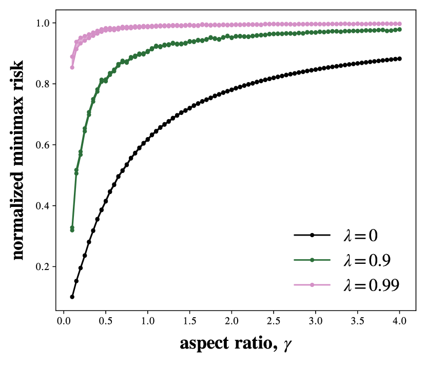
(a) $n=128,~{}\tau=1$

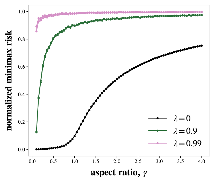
(b) $n=128,~{}\tau=10$

(c) $n=512,~{}\tau=1$

(d) $n=512,~{}\tau=10$

Figure 1: Simulations of random design regression for three covariate laws, $P_{\lambda}$ as defined in equation (72) with $\lambda\in\{0,0.9,0.99\}$. For a given choice of the mixture weight $\lambda$ and signal-to-noise ratio (SNR) $\tau$, we plot the lower bound $\ell_{n}(\lambda,\tau,\gamma)$ and upper bound $u_{n}(\lambda,\tau,\gamma)$ as $\gamma$ varies between $0.05$ and $4$. The normalized minimax risk $\mathfrak{m}_{n}$ is then guaranteed to lie in the region whose upper and lower envelopes are given by $u_{n}$ and $\ell_{n}$, respectively. To facilitate interpretation of these figures, we have shaded this region to highlight where we can guarantee the minimax risk $\mathfrak{m}_{n}$ must lie. The quantities $u_{n},\ell_{n},\mathfrak{m}_{n}$ are all defined in display (75). In panels (1(a)) and (1(b)), we set the sample size $n=128$, and set the SNR as $\tau=1,10$, respectively. In panels (1(c)) and (1(d)), we set the sample size $n=512$, and set the SNR as $\tau=1,10$, respectively. The plots above demonstrate that as $\lambda$ increases, the minimax risks are much worse. Numerically, in the setting where $n=512$ and $\tau=10$—as depicted in panel (1(d))—our upper and lower bounds guarantee that the minimax risk for the isotropic ensemble (depicted with $\lambda=0$ above) can be over 806 times larger than the minimax risk for the ensemble with $\lambda=0.99$. It should be noted that in this comparison the first and second moments of the ensemble are held fixed (see equation (73)), and hence the differences between the lines plotted in any given panel can only be explained by differences in higher-order moments within the ensemble $\{P_{\lambda}\}$. The figures also demonstrate that the gap between our upper and lower bounds is fairly small, particularly whenever $d>5$.

5.1.2 Mixing time effects in Markovian linear regression

Covariates need not be drawn in an IID manner, and any dependencies can be expected to affect the minimax risk. Here we illustrate this general phenomena via some simulations for the Markov regression example as outlined in Section 3.1.4. We seek to study a wide range of possible mixing conditions for the Markovian covariate model. In order to do so, we consider covariates generated from the Markovian model (26) with

$$r_{t}=\frac{\psi(t-1)}{\psi(t)},$$

where $\psi\colon\mathbf{N}\cup\{0\}\to\mathbf{R}_{+}$ is a nondecreasing function satisfying $\psi(0)=1$ and $\lim_{t\to\infty}\psi(t)=\infty$. With this choice, it is easily checked that, marginally

$$x_{t}\sim\mathsf{N}\left(0,1-\frac{1}{\psi(t)}\right).$$

Therefore, $x_{t}\to\mathsf{N}\left(0,1\right)$ in distribution as $t\to\infty$, and the rate of convergence is of order $1/\psi(t)$.

We now illustrate how the minimax rate, as determined in Corollary 5, for this problem behaves for different choices of the function $\psi$ and the signal-to-noise ratio (SNR). As in Section 5.1.1, we normalize the minimax risk by the squared radius so that it only depends on $\tau=\tfrac{\varrho}{\sigma}$. The quantity we then plot is

$$\Phi_{T}(\tau)\coloneq\frac{\Phi_{T}(\tau,1)}{\tau^{2}},$$

where $\Phi_{T}(\varrho,\sigma)$ is the functional appearing in Corollary 5.

In the simulation, we consider the following choices of scaling function $\psi$,

$$5^{t},\quad t+1,\quad 1+\log(t+1),\quad\mbox{and}\quad 1+\log\big{(}1+\log(t+1)\big{)}.$$

With the choice $\psi(t)=5^{t}$, the underlying Markov chain converges geometrically to the standard Normal law. On the other hand, the choice $\psi(t)=\log(1+\log(1+t))+1$ exhibits much slower convergence—the variational distance between the law of $x_{t}$ and $\mathsf{N}\left(0,1\right)$ is of order $O(1/(\log\log t))$.

We simulate each of these chains, computing the normalized functional $\Phi_{T}(\tau)$ over the course of 5000 Monte Carlo trials. The sample size $T$ is varied between 10 and $3162$. In the simulation we also include the choice $r_{t}\equiv 0$, which corresponds to IID covariates. The results of the simulation are presented in Figure 2; see the caption for more details and commentary.

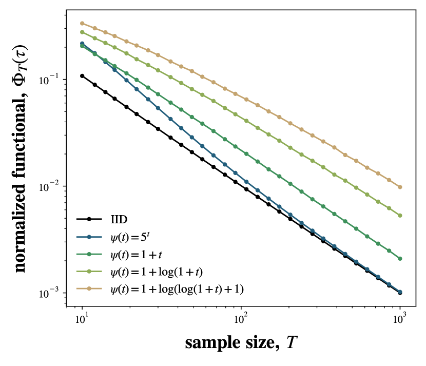
(a) $\tau=1$

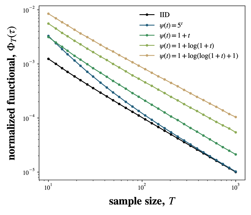
(b) $\tau=10$

Figure 2: Simulations for five distributions of Markovian covariates. In panel (2(a)), we set the SNR parameter as $\tau=1$, and in panel (2(b)), we set the SNR parameter as $\tau=10$. As the scaling function $\psi$ grows more slowly, the chain converges to its stationary distribution more slowly, and the minimax rate decays more slowly, as indicated by the displayed behavior of our functional $T\mapsto\Phi_{T}(\tau)$.

Acknowledgements

We thank Jaouad Mourtada for a helpful conversation and useful email exchanges; we also thank Peter Bickel for a helpful discussion regarding his prior work on the Gaussian sequence model. RP was partially supported by a UC Berkeley Chancellor’s Fellowship via the ARCS Foundation. MJW and RP were partially funded by ONR grant N00014-21-1-2842 and National Science Foundation grant NSF-DMS grant 2015454. MJW and RP gratefully acknowledge funding support from Meta via the UC Berkeley AI Research (BAIR) Commons initiative.

Appendix A Proofs from Section 2

A.1 Proof of Proposition 1

The constraint set is evidently convex, as it is formed by the intersection of of two convex sets: the $d\times d$ real, symmetric positive definite matrices with the hyperplane $\{\Omega:\operatorname{\bf Tr}({K_{c}}^{-1}\Omega)\leqslant\varrho^{2}\}$.

We claim that the objective function $f$ is concave over the set of symmetric positive definite matrices. It can be expressed as

$$f(\Omega)=\operatorname*{\mathbf{E}}\ilimits@_{\xi}[g(T_{\xi}^{\mathsf{T}}\Sigma_{w}^{-1}T_{\xi},\Omega)],\quad\mbox{where}\quad g(X,\Omega)\coloneq\operatorname{\bf Tr}({K_{e}}^{\!1/2}(X+\Omega^{-1})^{-1}{K_{e}}^{\!1/2}).$$

Evidently to establish that $f$ is concave, it is enough to show that $g(X,\cdot)$ is concave for every symmetric positive semidefinite $X$. In order to establish this claim, let us fix some $\varepsilon>0$, and define $X(\varepsilon)\coloneq X+\varepsilon I_{d}$. By the joint concavity of the harmonic mean of positive operators [61, Corollary 37.2], it follows that for any pair of positive definite matrices $\Omega,\Omega^{\prime}$, we have

$$\Big{(}X(\varepsilon)+\Big{(}\frac{\Omega+\Omega^{\prime}}{2}\Big{)}^{-1}\Big{)}^{-1}\succcurlyeq\frac{1}{2}\Big{(}X(\varepsilon)+\Omega^{-1}\Big{)}^{-1}+\frac{1}{2}\Big{(}X(\varepsilon)+(\Omega^{\prime})^{-1}\Big{)}^{-1}.$$

Passing to the limit as $\varepsilon\to 0$ yields

$$\Big{(}X+\Big{(}\frac{\Omega+\Omega^{\prime}}{2}\Big{)}^{-1}\Big{)}^{-1}\succcurlyeq\frac{1}{2}\Big{(}X+\Omega^{-1}\Big{)}^{-1}+\frac{1}{2}\Big{(}X+(\Omega^{\prime})^{-1}\Big{)}^{-1}.$$

Since the trace is a monotone mapping on positive definite matrices, and $g$ is continuous in its second argument, we obtain the claimed concavity of $g$.

A.2 Proof of Proposition 2

To establish the upper bound, it suffices to show that for each positive definite $\Omega\succ 0$ with $\operatorname{\bf Tr}({K_{c}}^{-1/2}\Omega{K_{c}}^{-1/2})\leqslant\frac{n\varrho^{2}}{\sigma^{2}}$ that the following inequality holds

$$\operatorname{\bf Tr}\Big{(}\operatorname*{\mathbf{E}}\ilimits@\big{[}\big{(}\Sigma_{n}+\Omega^{-1}\big{)}^{-1}\Sigma_{P}\big{]}\Big{)}\leqslant\Big{(}1+\frac{\varrho^{2}\kappa^{2}}{\sigma^{2}}\Big{)}\operatorname{\bf Tr}\big{(}\big{(}\Sigma_{P}+\Omega^{-1}\big{)}^{-1}\Sigma_{P}\Big{)}.$$ (76)

Our proof of the auxiliary claim (76) is based on exchangeability and operator convexity, and is similar to previous work on the analysis of ridge regression estimators [54]. Let $x_{n+1}$ be a fresh sample drawn independently from $\{x_{i}\}_{i=1}^{n}$ with the same distribution $P$. Letting $\operatorname*{\mathbf{E}}\ilimits@$ denote the expectation over the full sequence $\{x_{i}\}_{i=1}^{n+1}$, we have

$$\operatorname*{\mathbf{E}}\ilimits@\big{[}\big{(}\Sigma_{n}+\Omega^{-1}\big{)}^{-1}\Sigma_{P}\big{]}=n\operatorname*{\mathbf{E}}\ilimits@\big{[}\big{(}n\Sigma_{n}+n\Omega^{-1}\big{)}^{-1}(\psi(x_{n+1})\otimes\psi(x_{n+1}))\big{]}.$$ (77)

Define $\hat{\Sigma}_{n+1}\coloneq(n+1)^{-1}\sum_{i=1}^{n+1}\psi(x_{i})\otimes\psi(x_{i})$. Then, by the Sherman–Morrison lemma [34, Section 0.7.4], it follows that

$$(n\Sigma_{n}+n\Omega^{-1})^{-1}\psi(x_{n+1})=(1+\langle(n\Sigma_{n}+n\Omega^{-1})^{-1}\psi(x_{n+1}),\psi(x_{n+1})\rangle\big{(}(n+1)\hat{\Sigma}_{n+1}+n\Omega^{-1}\big{)}^{-1}\psi(x_{n+1}).$$

Additionally, by the Cauchy–Schwarz inequality, we have

$$\langle(n\Sigma_{n}+n\Omega^{-1})^{-1}\psi(x_{n+1}),\psi(x_{n+1})\rangle\leqslant\frac{1}{n}\vvvert{K_{c}}^{\!-1/2}\Omega\vvvert_{\rm op}\|{K_{c}}^{1/2}\psi(x_{n+1})\|_{2}^{2}\leqslant\frac{\varrho^{2}\kappa^{2}}{\sigma^{2}},$$

where the last inequality holds $P$-almost surely. Applying the previous two displays in relation (77), it follows that

$$\operatorname{\bf Tr}\operatorname*{\mathbf{E}}\ilimits@\big{[}\big{(}\Sigma_{n}+\Omega^{-1}\big{)}^{-1}\Sigma_{P}\big{]} \leqslant\Big{(}1+\frac{\varrho^{2}\kappa^{2}}{\sigma^{2}}\Big{)}\operatorname{\bf Tr}\operatorname*{\mathbf{E}}\ilimits@\big{[}\big{(}\hat{\Sigma}_{n+1}+\Omega^{-1}\big{)}^{-1}\psi(x_{n+1})\otimes\psi(x_{n+1})\big{]}$$

$$=\Big{(}1+\frac{\varrho^{2}\kappa^{2}}{\sigma^{2}}\Big{)}\frac{1}{n+1}\sum_{i=1}^{n+1}\operatorname{\bf Tr}\operatorname*{\mathbf{E}}\ilimits@\big{[}\big{(}\hat{\Sigma}_{n+1}+\Omega^{-1}\big{)}^{-1}\psi(x_{i})\otimes\psi(x_{i})\big{]}$$ (78)

$$=\Big{(}1+\frac{\varrho^{2}\kappa^{2}}{\sigma^{2}}\Big{)}\operatorname{\bf Tr}\operatorname*{\mathbf{E}}\ilimits@\big{[}\big{(}\hat{\Sigma}_{n+1}+\Omega^{-1}\big{)}^{-1}\hat{\Sigma}_{n+1}\big{]}$$ (79)

$$\leqslant\Big{(}1+\frac{\varrho^{2}\kappa^{2}}{\sigma^{2}}\Big{)}\operatorname{\bf Tr}\Big{(}\big{(}\Sigma_{P}+\Omega^{-1}\big{)}^{-1}\Sigma_{P}\Big{)}.$$ (80)

Above step (79) follows by the exchangeability of $\{\psi(x_{i})\}_{i=1}^{n+1}$, and step (80) follows by the cyclicity and linearity of the trace, as well as the the fact that for any fixed symmetric positive definite matrix $B$, the mapping $A\mapsto(A+B)^{-1}A=I_{d}-(A+B)^{-1}B$ is concave over the set over symmetric positive semidefinite matrices (see Bhatia [8, page 19]).

A.3 Proof of Corollary 2

Combining Theorems 2 and 2, we find that

$$\Phi(T,\mathbb{P},\Sigma_{w},\tfrac{\varrho}{2},{K_{e}},{K_{c}})\leqslant\mathfrak{M}(T,\mathbb{P},\Sigma_{w},\varrho,{K_{e}},{K_{c}})\leqslant\Phi(T,\mathbb{P},\Sigma_{w},\varrho,{K_{e}},{K_{c}}).$$ (81)

Evidently, by definition of the functional $\Phi$ (see definition (5)), the map $\varrho\to\Phi(T,\mathbb{P},\Sigma_{w},\varrho,{K_{e}},{K_{c}})$ is nondecreasing. Moreover since $T_{\xi}^{\mathsf{T}}\Sigma_{w}^{-1}T_{\xi}$ is invertible with probability 1, it is a bounded function. Therefore,

$$\lim_{\varrho\to\infty}\frac{\Phi(T,\mathbb{P},\Sigma_{w},\varrho,{K_{e}},{K_{c}})}{\Phi(T,\mathbb{P},\Sigma_{w},\varrho/2,{K_{e}},{K_{c}})}=1,$$

which in view of the sandwich relation (81), furnishes the claim.

Appendix B Proofs and calculations from Section 3

B.1 Proof and calculations from Section 3.1

B.1.1 Proof of equation (21a)

From the definition of the functional (13), we have

$$d_{n}(\mathsf{N}\left(0,I_{d}\right),\varrho,\sigma^{2},I_{d},I_{d})=\sup\Big{\{}\,\operatorname*{\mathbf{E}}\ilimits@[\operatorname{\bf Tr}((\Sigma_{n}+\tfrac{\sigma^{2}d}{n\varrho^{2}}M^{-1})^{-1})]:M\succ 0,~{}~{}\operatorname{\bf Tr}(M)=d\,\Big{\}}.$$

In this section, all expectations are over $x_{i}\stackrel{{\scriptstyle\rm IID}}{{\sim}}\mathsf{N}\left(0,I_{d}\right)$. We claim that the supremum above is achieved at $M=I_{d}$.

Lemma 8.

For any positive definite matrix $M\succ 0$ such that $\operatorname{\bf Tr}(M)=d$, we have

$$\operatorname*{\mathbf{E}}\ilimits@[\operatorname{\bf Tr}((\Sigma_{n}+\tfrac{\sigma^{2}d}{n\varrho^{2}}M^{-1})^{-1})]\leqslant\operatorname*{\mathbf{E}}\ilimits@[\operatorname{\bf Tr}((X^{\mathsf{T}}X+\tfrac{d\sigma^{2}}{\varrho^{2}}I_{d})^{-1})]$$

Assuming Lemma 8, we then have

$$d_{n}(\mathsf{N}\left(0,I_{d}\right),\varrho,\sigma^{2},I_{d},I_{d})=\operatorname*{\mathbf{E}}\ilimits@[\operatorname{\bf Tr}((\Sigma_{n}+\tfrac{\sigma^{2}d}{n\varrho^{2}}I_{d})^{-1})]=d_{\rm Dicker}(n,d,\varrho,\sigma),$$

which establishes (21a), as needed.

Proof of Lemma 8

Define the function $\phi\colon(\Sigma,M)\mapsto(\Sigma+\tfrac{d\sigma^{2}}{n\varrho^{2}}M^{-1})^{-1}$, where $\Sigma,M$ are assumed symmetric positive semidefinite and $M$ is nonsingular. For each $\Sigma\succcurlyeq 0$, it is well known that $\phi(\Sigma,\cdot)$ is operator concave [61, Corollary 37.2]—for any collection $\{M_{i}\}_{i=1}^{d}$ of symmetric positive definite matrices, one has

$$\frac{1}{d}\sum_{i=1}^{d}\phi(\Sigma,M_{i})\preccurlyeq\phi(\Sigma,\tfrac{1}{d}\sum_{i=1}^{d}M_{i}),\qquad\mbox{for any}~{}\Sigma\in\mathbb{S}_{+}^{d}.$$ (82)

Now let $M\succ 0$ satisfying $\operatorname{\bf Tr}(M)=d$ be given. Diagonalize $M$ so that $M=U\Lambda U^{\mathsf{T}}$, where $\Lambda=\operatorname{\bf diag}(\lambda)\succ 0$, and $U$ is orthogonal. Consider the cyclic permutations of $\Lambda$, given by

$$\Lambda^{(j)}=\operatorname{\bf diag}(\lambda^{(j)}),\quad\mbox{where}\quad\lambda^{(j)}_{i}=\lambda_{i+j}.$$

Above, the arithmetic $i+j$ occurs modulo $d$. By rotational invariance of the Gaussian and the fact that $x_{i}$ has iid coordinates, we have

$$\operatorname*{\mathbf{E}}\ilimits@\operatorname{\bf Tr}((\Sigma_{n}+\tfrac{d\sigma^{2}}{n\varrho^{2}}M^{-1})^{-1}) =\operatorname*{\mathbf{E}}\ilimits@\operatorname{\bf Tr}((\Sigma_{n}+\tfrac{d\sigma^{2}}{n\varrho^{2}}\Lambda^{-1})^{-1})$$

$$=\operatorname*{\mathbf{E}}\ilimits@\Big{[}\frac{1}{d}\sum_{j=1}^{d}\operatorname{\bf Tr}((\Sigma_{n}+\tfrac{d\sigma^{2}}{n\varrho^{2}}(\Lambda^{(j)})^{-1})^{-1})\Big{]}$$

$$=\operatorname{\bf Tr}\Big{\{}\operatorname*{\mathbf{E}}\ilimits@\Big{[}\frac{1}{d}\sum_{j=1}^{d}\phi(\Sigma_{n},\Lambda^{(j)})\Big{]}\Big{\}}$$

$$\leqslant\operatorname{\bf Tr}\Big{\{}\operatorname*{\mathbf{E}}\ilimits@\Big{[}\phi(\Sigma_{n},\overline{\Lambda})\Big{]}\Big{\}}\qquad\mbox{where}\quad\overline{\Lambda}\coloneq\tfrac{1}{d}\sum_{j=1}^{d}\Lambda^{(j)},$$

The final inequality above uses the concavity inequality (82), where we have taken $M_{i}=\Lambda^{(i)}$. Now note that

$$\overline{\Lambda}=\frac{\operatorname{\bf Tr}(\Lambda)}{d}I_{d}=\frac{\operatorname{\bf Tr}(M)}{d}I_{d}=I_{d}.$$

Combining the preceding displays furnishes the claim.

B.1.2 Proof of the lower bound in equation (20a)

We apply our our sharp lower bound in Theorem 2 with $\Omega=\tfrac{\varrho^{2}}{d}I_{d}$ and $\tau^{2}=1-\tfrac{1}{2d-1}$. Let us define $u=(1-\tfrac{1}{2d-1})(1-\operatorname*{\mathbf{P}}\ilimits@\{Z>2d^{2}-d\})$, where $Z$ is a $\chi^{2}$-random variable with $d$-degrees of freedom. Note that $d(d-1)\geqslant\sqrt{dt}+t$ for $t=\tfrac{d^{3/2}}{4}$ for all $d\geqslant 2$. Therefore by standard tail bounds for $\chi^{2}$-variates [42, pp. 1325], we have $u\leqslant\exp(-d^{3/2}/4)$. Applying the sharp lower bound (8) in Theorem 2 then yields the claim.

B.1.3 Proof of equation (25)

Using the semidefinite inequality

$$\big{(}\Sigma_{n}+\Omega^{-1}\big{)}^{-1}\preccurlyeq\Sigma_{n}^{-1},$$

and the choice $\Omega=\tfrac{n}{\sigma^{2}}\tfrac{\varrho^{2}}{d}I_{d}$, we have the sandwich relation

$$\operatorname{\bf Tr}\operatorname*{\mathbf{E}}\ilimits@_{P^{n}}\big{[}\Sigma_{P}^{1/2}(\Sigma_{n}+\tfrac{\sigma^{2}}{n}\tfrac{d}{\varrho^{2}}I_{d})^{-1}\Sigma_{P}^{1/2}\big{]}\leqslant d_{n}(P,\varrho,\sigma^{2},I_{d},\Sigma_{P})\leqslant\operatorname{\bf Tr}\operatorname*{\mathbf{E}}\ilimits@_{P^{n}}\big{[}\Sigma_{P}^{1/2}\Sigma_{n}^{-1}\Sigma_{P}^{1/2}\big{]},$$ (83)

for all $\varrho>0$. Since $\varrho\mapsto d_{n}(P,\varrho,\sigma^{2},I_{d},\Sigma_{P})$ is nondecreasing, the display above also demonstrates that this map has a limit. Now, note that by continuity, $P^{n}$-almost surely we have

$$\lim_{\varrho\to\infty}\operatorname{\bf Tr}(\Sigma_{P}^{1/2}(\Sigma_{n}+\tfrac{\sigma^{2}}{n}\tfrac{d}{\varrho^{2}}I_{d})^{-1}\Sigma_{P}^{1/2})=\operatorname{\bf Tr}(\Sigma_{P}^{1/2}\Sigma_{n}^{-1}\Sigma_{P}^{1/2}).$$

Thus, using the sandwich relation (25) and Fatou’s lemma, we have

$$\operatorname{\bf Tr}\operatorname*{\mathbf{E}}\ilimits@_{P^{n}}\big{[}\Sigma_{P}^{1/2}\Sigma_{n}^{-1}\Sigma_{P}^{1/2}\big{]}\leqslant\liminf_{\varrho\to\infty}\operatorname{\bf Tr}\operatorname*{\mathbf{E}}\ilimits@_{P^{n}}\big{[}\Sigma_{P}^{1/2}(\Sigma_{n}+\tfrac{\sigma^{2}}{n}\tfrac{d}{\varrho^{2}}I_{d})^{-1}\Sigma_{P}^{1/2}\big{]}\\ \leqslant\lim_{\varrho\to\infty}d_{n}(P,\varrho,\sigma^{2},I_{d},\Sigma_{P})\leqslant\operatorname{\bf Tr}\operatorname*{\mathbf{E}}\ilimits@_{P^{n}}\big{[}\Sigma_{P}^{1/2}\Sigma_{n}^{-1}\Sigma_{P}^{1/2}\big{]},$$

which establishes relation (25), as required.

B.1.4 Proof of minimax relation (29)

Let us state the claim corresponding to relation (29) somewhat more precisely. We define the functional

$$\Phi_{T}(\varrho,\sigma)\coloneq\operatorname*{\mathbf{E}}\ilimits@\bigg{[}\Big{(}\frac{1}{\varrho^{2}}+\frac{z^{\mathsf{T}}Mz}{\sigma^{2}}\Big{)}^{-1}\bigg{]}$$

Then the following lemma corresponds to the claim underlying relation (29).

Lemma 9.

The minimax risk under the Markovian observation model defined by the displays (26) and (27) satisfies

$$\frac{1}{4}\,\Phi_{T}(\varrho,\sigma)\leqslant\inf_{\widehat{\theta}}\sup_{|\theta^{\star}|\leqslant\varrho}\operatorname*{\mathbf{E}}\ilimits@\big{[}(\widehat{\theta}-\theta^{\star})^{2}\big{]}\leqslant\Phi_{T}(\varrho,\sigma).$$

The remainder of this section is devoted to the proof of this claim

Note that if we define $\xi=(x_{1},\dots,x_{T})$, and $T_{\xi}=x$, then the observation model (27) can be written

$$y=T_{\xi}\theta^{\star}+\Sigma_{w}^{1/2}w,$$

where $w\sim\mathsf{N}\left(0,I_{T}\right)$ and $\Sigma_{w}=\sigma^{2}I_{T}$. We have ${K_{c}}=1={K_{e}}$, since we are considering a univariate estimation problem. Therefore, since the functional (5) is attained at $\Omega=\varrho^{2}$, in order to establish Lemma 9, it is sufficient to show that

$$T_{\xi}^{\mathsf{T}}\Sigma_{w}^{-1}T_{\xi}=\frac{x^{\mathsf{T}}x}{\sigma^{2}}=\frac{z^{\mathsf{T}}Mz}{\sigma^{2}}.$$ (84)

However, from display (26), by induction we can establish that

$$x_{t}=\sum_{s=1}^{t}\sqrt{c_{st}}\,z_{s},$$

where the coefficients $\{c_{st}\}$ are defined as in display (28). Then, it follows that

$$x^{\mathsf{T}}x=\sum_{t=1}^{T}\sum_{s,s^{\prime}=1}^{t}\sqrt{c_{st}c_{s^{\prime}t}}z_{s}z_{s^{\prime}}=\sum_{s,s^{\prime}=1}^{T}\underbrace{\sum_{t=s\lor s^{\prime}}\sqrt{c_{st}c_{s^{\prime}t}}}_{=M_{ss^{\prime}}}z_{s}z_{s^{\prime}}.$$

Using the display above, we establish the relation (84), which in turn establishes Lemma 9, as needed.

B.2 Proof and calculations from Section 3.2

B.2.1 Proof of limit relation (31)

To lighten notation in this section, let us define the shorthands

$$\mathfrak{M}_{k} \coloneq\mathfrak{M}_{k}\Big{(}\{\varepsilon_{j}\}_{j=1}^{k},\Theta_{k}(a,C)\Big{)},\quad\mbox{and,}$$ (85a)

$$\mathfrak{M} \coloneq\mathfrak{M}\Big{(}\{\varepsilon_{j}\}_{j=1}^{\infty},\Theta(a,C)\Big{)}\coloneq\inf_{\widehat{\theta}}\sup_{\theta^{\star}\in\Theta(a,C)}\operatorname*{\mathbf{E}}\ilimits@\Big{[}\sum_{j=1}^{\infty}(\widehat{\theta}_{j}(y)-\theta^{\star}_{j})^{2}\Big{]}.$$ (85b)

We begin by stating the following sandwich relation for the minimax risks.

Lemma 10.

The sequence of minimax risks $\{\mathfrak{M}_{k}\}$ and infinite-dimensional risk $\mathfrak{M}$ satisfies the sandwich relation

$$\mathfrak{M}_{k}\leqslant\mathfrak{M}\leqslant\mathfrak{M}_{k}+\frac{C^{2}}{a_{k+1}^{2}},$$ (86)

for all $k\geqslant 1$.

Assuming Lemma 10 for the moment, note that it implies for any divergent sequence $a_{k}\to\infty$ that

$$\lim_{k\to\infty}\mathfrak{M}_{k}=\mathfrak{M}.$$

In view of the shorthands (85), the display above establishes our desired limit relation (31).

Proof of Lemma 10

We begin by establishing the lower bound. Note that $\Theta_{k}(a,C)\subset\Theta(a,C)$, hence we have

$$\mathfrak{M} \geqslant\inf_{\widehat{\theta}}\sup_{\theta^{\star}\in\Theta_{k}(a,C)}\operatorname*{\mathbf{E}}\ilimits@\Big{[}\sum_{j=1}^{\infty}(\widehat{\theta}_{j}((y_{i})_{i=1}^{\infty})-\theta^{\star}_{j})^{2}\Big{]}$$

$$\geqslant\inf_{\widehat{\theta}}\sup_{\theta^{\star}\in\Theta_{k}(a,C)}\operatorname*{\mathbf{E}}\ilimits@\Big{[}\sum_{j=1}^{k}(\widehat{\theta}_{j}((y_{i})_{i=1}^{\infty})-\theta^{\star}_{j})^{2}\Big{]},$$

where the last equation arises since $\theta^{\star}_{j}=0$ for $j>k$ and thus any minimax optimal estimator over $\Theta_{k}(a,C)$ satisfies $\widehat{\theta}_{j}\equiv 0$ for all $j>k$. The righthand side differs from $\mathfrak{M}_{k}$ in that $\widehat{\theta}$ is a function of the full sequence $y=(y_{i})_{i=1}^{\infty}$. However, note that due to the independence of the noise variables $z_{i}$, for the observation model (30) restricted to $\Theta_{k}(a,C)$, the vector $y^{(k)}=(y_{i})_{i=1}^{k}$ is a sufficient statistic. Hence we have for each $k\geqslant 1$,

$$\mathfrak{M}\geqslant\inf_{\widehat{\theta}}\sup_{\theta^{\star}\in\Theta_{k}(a,C)}\operatorname*{\mathbf{E}}\ilimits@\Big{[}\sum_{j=1}^{k}(\widehat{\theta}_{j}(y^{(k)})-\theta^{\star}_{j})^{2}\Big{]}=\mathfrak{M}_{k},$$

which establishes the lower bound in relation (86).

To establish the upper bound, note that we certainly may restrict the infimum in the definition of $\mathfrak{M}$ to those estimators taking values in $\mathbf{R}^{k}$ which only are a function of $y^{(k)}$. Indeed, we then find

$$\mathfrak{M} \leqslant\inf_{\widehat{\theta}\in\mathbf{R}^{k}}\sup_{\theta^{\star}\in\Theta(a,C)}\operatorname*{\mathbf{E}}\ilimits@\Big{[}\sum_{j=1}^{k}(\widehat{\theta}_{j}(y^{(k)})-\theta^{\star}_{j})^{2}+\sum_{j>k}(\theta^{\star}_{j})^{2}\Big{]}$$ (87)

$$\leqslant\mathfrak{M}_{k}+\sup_{\theta^{\star}\in\Theta(a,C)}\sum_{j>k}(\theta^{\star}_{j})^{2}.$$ (88)

The inequality (88) arises by taking the supremum over the two terms of the risk in display (87), and noting the first term only depends on the first $k$ coordinate of $\theta^{\star}\in\Theta(a,C)$, and hence the supremum may be taken over $\Theta_{k}(a,C)$ in the first term so as to obtain $\mathfrak{M}_{k}$.

Now observe by Hölder’s inequality, and the membership $\theta^{\star}\in\Theta(a,C)$,

$$\sum_{j>k}(\theta^{\star}_{j})^{2}=\sum_{j>k}\frac{1}{a_{j}^{2}}(a_{j}^{2}(\theta^{\star}_{j})^{2})\leqslant\Big{(}\max_{j>k}\frac{1}{a_{j}^{2}}\Big{)}C^{2}=\frac{C^{2}}{a_{k+1}^{2}},$$

with the last equality arising because $j\mapsto a_{j}^{2}$ is assumed nondecreasing. Combining the display above with inequality (88) establishes the upper bound in (86), and thus establishes Lemma 10 as needed.

B.2.2 Proof of relation (35)

Let us continue to adopt the shorthands $\mathfrak{M}_{k}$ and $\mathfrak{M}$ defined, respectively, in the displays (85a) and (85b). Moreover, we also use the shorthands

$$R_{k}^{\star}\coloneq R_{k}^{\star}\Big{(}\varepsilon,a,C\Big{)},\quad\mbox{and}\quad R^{\star}\coloneq R^{\star}(\varepsilon,a,C),$$

corresponding to the functionals (33) and (34), respectively.

We prove the following lemma.

Lemma 11.

The functionals $R_{k}^{\star}$, $R^{\star}$ and minimax risks $\mathfrak{M}_{k}$ satisfy

$$\frac{1}{4}R_{k}^{\star} \leqslant\mathfrak{M}_{k}\leqslant R_{k}^{\star}\quad\mbox{for all $k\geqslant 1$, and,}$$ (89a)

$$\lim_{k\to\infty}R_{k}^{\star}=R^{\star}.$$ (89b)

Assuming Lemma 11 for the moment, note that the two inequalities immediately imply the sandwich relation (35), simply by applying the sandwich (89a) to the terms $\mathfrak{M}_{k}$ and then applying the limit relations (31) and (89b). Consequently, it suffices to establish Lemma 11.

Proof of Lemma 11

Recall the settings of the parameters $T^{(k)},\Sigma_{w}^{(k)},{K_{e}}^{(k)},\varrho^{(k)},{K_{c}}^{(k)}$, corresponding to the $k$ dimensional minimax risk $\mathfrak{M}_{k}$, as given in (32). We claim that

$$\Phi(T^{(k)},\mathbb{P},\Sigma_{w}^{(k)},\varrho^{(k)},{K_{e}}^{(k)},{K_{c}}^{(k)})=R_{k}^{\star}.$$ (90)

(Note by our construction of $T^{(k)}$ the choice of $\mathbb{P}$ is irrelevant.) Then the sandwich relation (89a) follows by applying Theorems 1 and 2 to the minimax risk $\mathfrak{M}_{k}$.

To see that relation (90) holds, note that by definition 5, we have

$$\Phi(T^{(k)},\mathbb{P},\Sigma_{w}^{(k)},\varrho^{(k)},{K_{e}}^{(k)},{K_{c}}^{(k)})=\sup_{\Omega\succ 0}\Big{\{}\,\operatorname{\bf Tr}\Big{(}(\Omega^{-1}+(\Sigma_{w}^{(k)})^{-1})^{-1}\Big{)}:\sum_{j=1}^{k}a_{j}^{2}\Omega_{jj}\leqslant C^{2}\,\Big{\}}.$$

We claim that the supremum above can be reduced to diagonal $\Omega$. To see why, first note that for every nonzero $\lambda\in\mathbf{R}$

$$\big{(}\Omega^{-1}+(\Sigma_{w}^{(k)})^{-1}\big{)}^{-1}\preccurlyeq\lambda^{2}\Omega+(1-\lambda)^{2}\Sigma_{w}^{(k)}.$$

This follows from Lemma 15, with the choices

$$A=\Sigma_{w}^{(k)},\quad B=\Omega^{-1},\quad\mbox{and}\quad D=\lambda I.$$

Consequently, we have for every nonzero $u\in\mathbf{R}^{k}$, that

$$u^{\mathsf{T}}\big{(}\Omega^{-1}+(\Sigma_{w}^{(k)})^{-1}\big{)}^{-1}u\leqslant\inf_{\lambda\in\mathbf{R}}\lambda^{2}u^{\mathsf{T}}\Omega u+(1-\lambda)^{2}u^{\mathsf{T}}\Sigma_{w}^{(k)}u=\Big{(}\frac{1}{u^{\mathsf{T}}\Omega u}+\frac{1}{u^{\mathsf{T}}\Sigma_{w}^{(k)}u}\Big{)}^{-1}.$$

Hence taking $u$ to be elements of the standard basis $e_{i}$, and summing over $i=1,\dots,k$, we obtain,

$$\operatorname{\bf Tr}\Big{(}\big{(}\Omega^{-1}+(\Sigma_{w}^{(k)})^{-1}\big{)}^{-1}\Big{)}\leqslant\sum_{i=1}^{k}\Big{(}\frac{1}{\Omega_{ii}}+\frac{1}{\varepsilon_{i}^{2}}\Big{)}^{-1}=\sum_{i=1}^{k}\frac{\Omega_{ii}\varepsilon_{i}^{2}}{\Omega_{ii}+\varepsilon_{i}^{2}}.$$

Moreover, by taking $\Omega$ to be diagonal, the inequality above holds with equality. Thus,

$$\Phi(T^{(k)},\mathbb{P},\Sigma_{w}^{(k)},\varrho^{(k)},{K_{e}}^{(k)},{K_{c}}^{(k)}) =\sup_{\Omega_{jj}>0}\Big{\{}\,\sum_{j=1}^{k}\frac{\Omega_{jj}\varepsilon_{j}^{2}}{\Omega_{jj}+\varepsilon_{j}^{2}}:\sum_{j=1}^{k}a_{j}^{2}\Omega_{jj}\leqslant C^{2}\,\Big{\}}$$

$$=\sup_{\tau_{j}^{2}>0}\Big{\{}\,\sum_{j=1}^{k}\frac{\tau_{j}^{2}\varepsilon_{j}^{2}}{\tau_{j}^{2}+\varepsilon_{j}^{2}}:\sum_{j=1}^{k}a_{j}^{2}\tau_{j}^{2}\leqslant C^{2}\,\Big{\}}$$

$$=R^{\star}_{k},$$

which establishes the relation (90). Note that in the last equality, we have dropped the inequality constraints $\tau_{j}^{2}>0$, due to the continuity of the map $\tau\mapsto\sum_{i=1}^{k}\frac{\tau_{j}^{2}\varepsilon_{j}^{2}}{\tau_{j}^{2}+\varepsilon_{j}^{2}}$ over $\tau\in\mathbf{R}^{k}$.

We now turn to establishing the relation (89b). Note that for any $\tau\in\mathbf{R}^{\mathbf{N}}$ with $\sum_{j=1}^{\infty}a_{j}^{2}\tau_{j}^{2}\leqslant C^{2}$, we have

$$\sum_{j=1}^{k}\frac{\tau_{j}^{2}\varepsilon_{j}^{2}}{\tau_{j}^{2}+\varepsilon_{j}^{2}}\leqslant\sum_{j=1}^{\infty}\frac{\tau_{j}^{2}\varepsilon_{j}^{2}}{\tau_{j}^{2}+\varepsilon_{j}^{2}}\leqslant\sum_{j=1}^{k}\frac{\tau_{j}^{2}\varepsilon_{j}^{2}}{\tau_{j}^{2}+\varepsilon_{j}^{2}}+\sup_{\tau\in\mathbf{R}^{\mathbf{N}}:\sum_{j=1}^{\infty}a_{j}^{2}\tau_{j}^{2}\leqslant C^{2}}\sum_{j>k}^{\infty}\tau_{j}^{2}$$

By Hölder’s inequality, the second term is bounded above by $C^{2}/a_{k+1}^{2}$, hence in view of definitions (33) and (34), we have the sandwich relation

$$R_{k}^{\star}\leqslant R^{\star}\leqslant R_{k}^{\star}+\frac{C^{2}}{a_{k+1}^{2}},$$

which holds for all $k\geqslant 1$. Since $a_{k}\to\infty$, the limit relation (89b) follows.

B.2.3 Proof of limit relation (42)

We claim that the following sandwich relation holds for the minimax risks in this case.

Lemma 12.

For all $k\geqslant 1$, we have

$$\mathfrak{M}^{(k)}_{n}(\varrho,\sigma^{2},P)\leqslant\mathfrak{M}_{n}(\varrho,\sigma^{2},P)\leqslant\mathfrak{M}^{(k)}_{n}(\varrho,\sigma^{2},P)+\varrho^{2}\mu_{k+1}.$$ (91)

Assuming Lemma 12, note that since $\mu_{k}\to 0$ as $k\to\infty$, it immediately implies limit relation (42)

Proof of Lemma 12

The proof is quite similar to Lemma 10. We now prove inequality (91). We begin by defining the sets

$$\mathcal{B}(\varrho)=\{\theta\in\ell^{2}(\mathbf{N}):\|\theta\|_{2}\leqslant\varrho\},\quad\mbox{and}\quad\mathcal{B}_{k}(\varrho)=\{\theta\in\mathcal{B}_{k}(\varrho):\theta_{j}=0,~{}~{}\mbox{for all}~{}j>k\}.$$

By Parseval’s identity, we may rewrite the minimax risks in the following form

$$\mathfrak{M}_{k} \equiv\mathfrak{M}^{(k)}_{n}(\varrho,\sigma^{2},P)=\inf_{\widehat{\theta}}\sup_{\begin{subarray}{c}\theta^{\star}\in\mathcal{B}_{k}(\varrho)\\ \nu\in\mathcal{P}(\sigma^{2}I_{n})\end{subarray}}\operatorname*{\mathbf{E}}\ilimits@\Big{[}\sum_{j=1}^{k}\mu_{j}(\widehat{\theta}_{j}(y_{1},\dots,y_{n},\Phi_{k}(x_{1}),\dots,\Phi_{k}(x_{n}))-\theta^{\star}_{j})^{2}\Big{]},$$ (92a)

$$\mathfrak{M} \equiv\mathfrak{M}_{n}(\varrho,\sigma^{2},P)=\inf_{\widehat{\theta}}\sup_{\begin{subarray}{c}\theta^{\star}\in\mathcal{B}(\varrho)\\ \nu\in\mathcal{P}(\sigma^{2}I_{n})\end{subarray}}\operatorname*{\mathbf{E}}\ilimits@\Big{[}\sum_{j=1}^{\infty}\mu_{j}(\widehat{\theta}_{j}(y_{1},\dots,y_{n},\Phi(x_{1}),\dots,\Phi(x_{n}))-\theta^{\star}_{j})^{2}\Big{]}.$$ (92b)

Evidently, we have $\mathfrak{M}\geqslant\mathfrak{M}_{k}$, since $\mathcal{B}_{k}(\varrho)\subset\mathcal{B}(\varrho)$ and $(y,\Phi_{k}(x))$ are sufficient in this submodel. Similarly, the upper bound follows since by restricting to those estimators $\widehat{\theta}$ with $\widehat{\theta}_{j}=0$ for all $j>k$ that are functions of $(y,\Phi_{k}(x))$, we have

$$\mathfrak{M}\leqslant\mathfrak{M}_{k}+\sup_{\theta\in\mathcal{B}(\varrho)}\sum_{j>k}\mu_{j}\theta_{j}^{2}=\mathfrak{M}_{k}+\varrho^{2}\mu_{k+1},$$

which establishes the upper bound.

B.2.4 Proof of relation (45)

Applying Corollary 1 to the minimax risk $\mathfrak{M}_{k}(\varrho,\sigma^{2},P)$, we find that

$$\frac{1}{4}\,\frac{\sigma^{2}}{n}d_{n}^{(k)}\leqslant\mathfrak{M}_{k}(\varrho,\sigma^{2},P)\leqslant\frac{\sigma^{2}}{n}d_{n}^{(k)},$$

since the quantity $d_{n}^{(k)}$ equals the functional for this minimax risk (see equation (44)). Therefore passing to the superior limit and applying the limit relation (42), we obtain the result.

B.2.5 Proof of relation (47)

First, we define the population counterparts of the functional $d_{n}^{(k)}$, as defined in equation (44). Note that under $P$, we have $\operatorname*{\mathbf{E}}\ilimits@\Sigma_{n}^{(k)}=\operatorname{\bf diag}(\mu_{1},\dots,\mu_{k})$. We denote this matrix by $M_{k}$. Hence, the population counterpart to $d_{n}^{(k)}$ is

$$\overline{d}_{n}^{(k)} \coloneq\sup_{\Omega\succ 0}\,\Big{\{}\operatorname{\bf Tr}\Big{(}M_{k}(M_{k}+\Omega^{-1})^{-1}\Big{)}:\operatorname{\bf Tr}(\Omega)\leqslant\frac{n\varrho^{2}}{\sigma^{2}}\Big{\}}$$ (93)

$$=\sup_{\Omega\succ 0}\,\Big{\{}\operatorname{\bf Tr}\Big{(}(I_{k}+\Omega^{-1})^{-1}\Big{)}:\operatorname{\bf Tr}(M_{k}^{-1}\Omega)\leqslant\frac{n\varrho^{2}}{\sigma^{2}}\Big{\}}.$$ (94)

Using Proposition 2 and the sandwich relation (91), we find

$$\frac{1}{4}\,\frac{\sigma^{2}}{n}\overline{d}_{n}^{(k)}\leqslant\mathfrak{M}_{n}^{(k)}(\varrho,\sigma^{2},P)\leqslant\Big{(}1+\frac{\kappa^{2}\varrho^{2}}{\sigma^{2}}\Big{)}\frac{\sigma^{2}}{n}\overline{d}_{n}^{(k)}+\mu_{k+1}\varrho^{2}.$$

Since $\mu_{k}\to 0$ as $j\to\infty$, it suffices to show that

$$\lim_{j\to\infty}\overline{d}_{n}^{(k)}=\overline{d}_{n}^{\star}.$$ (95)

Proof of relation (95)

This limit relation can be established via an argument based on Lagrange multipliers. First, by an eigendecomposition of the variable $\Omega\succ 0$, we have

$$\overline{d}_{n}^{(k)} =\sup\Big{\{}\sum_{j=1}^{k}\frac{\tau_{j}}{1+\tau_{j}}:\tau_{j}>0,\sum_{j=1}^{k}\frac{\tau_{j}}{\mu_{j}}\leqslant\frac{n\varrho^{2}}{\sigma^{2}}\Big{\}}$$

$$=\sup\Big{\{}\sum_{j=1}^{k}\frac{\mu_{j}\gamma_{j}}{\tfrac{\sigma^{2}}{n\varrho^{2}}+\mu_{j}\gamma_{j}}:\gamma_{j}\geqslant 0,\sum_{j=1}^{k}\gamma_{j}\leqslant 1\Big{\}}.$$ (96)

The final equality arises by a rescaling and continuity argument. Note that we may drop the nonnegativity constraint, since the sequence $\{\mu_{j}\}$ is nonnegative. We can compute (96) by introducing dual variables. In particular, we have

$$\overline{d}_{n}^{(k)} =\sup_{\gamma}\inf_{\lambda}\sum_{j=1}^{k}\frac{\mu_{j}\gamma_{j}}{\tfrac{\sigma^{2}}{n\varrho^{2}}+\mu_{j}\gamma_{j}}-\frac{\tfrac{n\varrho^{2}}{\sigma^{2}}}{\lambda^{2}}\Big{(}\sum_{j=1}^{k}\gamma_{j}-1\Big{)}.$$ (97)

By simple calculus, we see that the saddle point $(\gamma^{\star},\lambda^{\star})$ satisfies

$$\quad\sum_{j=1}^{k}\tau_{j}^{\star}=1\quad\mbox{and}\quad\Big{(}\frac{\sigma^{2}}{n\varrho^{2}}\Big{)}^{2}\frac{\mu_{j}}{(\tfrac{\sigma^{2}}{n\varrho^{2}}+\mu_{j}\gamma_{j}^{\star})^{2}}=\frac{1}{(\lambda^{\star})^{2}},~{}~{}\mbox{for}~{}j=1,\ldots,k.$$

Using the fact that $\gamma_{j}^{\star}\geqslant 0$, we obtain $\gamma_{j}^{\star}=\tfrac{\sigma^{2}}{n\varrho^{2}}\tfrac{1}{\sqrt{\mu_{j}}}(\lambda^{\star}-\tfrac{1}{\sqrt{\mu_{j}}})_{+}$, where $\lambda^{\star}$ is chosen such that

$$\frac{\sigma^{2}}{n\varrho^{2}}\sum_{j=1}^{k}\frac{1}{\sqrt{\mu_{j}}}\Big{(}\lambda^{\star}-\frac{1}{\sqrt{\mu_{j}}}\Big{)}_{+}=\frac{\sigma^{2}}{n\varrho^{2}}\sum_{j=1}^{k}\gamma^{\star}_{j}=1.$$

Using equation (96), it follows that

$$\overline{d}_{n}^{(k)}=\sum_{j=1}^{k}\frac{1}{\lambda^{\star}}\Big{(}\lambda^{\star}-\tfrac{1}{\sqrt{\mu_{j}}}\Big{)}_{+}.$$

The result then follows by appealing to the following numerical result, with $a_{j}=1/\sqrt{\mu_{j}}$.

Lemma 13.

Let $\{a_{j}\}_{j\geqslant 1}$ denote a nonnegative, divergent sequence, and define $a_{\star}\coloneq\inf_{j\geqslant 1}a_{j}$. Consider the functions $f_{n},f\colon[a_{\star},+\infty)\to\mathbf{R}_{+}$ given by

$$f_{n}(t)\coloneq\sum_{k=1}^{n}a_{k}(t-a_{k})_{+}\quad\mbox{and}\quad f(t)\coloneq\sum_{k=1}^{\infty}a_{k}(t-a_{k})_{+},$$

and define $\tau_{n}$ and $\tau$ via the relations $f_{n}(\tau_{n})=f_{n}(\tau)=1$. Then:

1. The function $f$ and values $\tau_{n},\tau$ are well-defined; and

2. We have $\tau_{n}=\tau$ for $n$ sufficiently large.

Proof of Lemma 13

Since the sequence $a_{k}$ diverges to infinity, we may assume without loss of generality that $a_{k}>0$ for all $k$. For the first claim, note that $f$ is well-defined. Indeed fix $t\geqslant a_{\star}$. Then, there exists $n$ sufficiently large such that $t<a_{k}$ for all $k\geqslant n$. Consequently, $f(t)=f_{n}(t)$. Similarly, note that $f_{n},f$ are strictly increasing, continuous functions with $f(a_{\star})=f_{n}(a_{\star})=0$, and $f(x),f_{n}(x)\to\infty$ in the limit as $x\to\infty$. Therefore, $\tau_{n},\tau$ exist and are uniquely defined by the equations $f_{n}(\tau_{n})=1$ and $f(\tau)=1$, respectively. By the argument given previously, $f_{n}(\tau)=f(\tau)$ for all $n$ large enough, and therefore, by uniqueness $\tau=\tau_{n}$ for $n$ large enough.

B.2.6 Proof of Sobolev rate calculation

Let $\{\mu_{j}\}_{j\geqslant 1}$ denote the eigenvalue sequence associated to the integral operator for the order $\beta$ Sobolev space on $[0,1]^{d}$. We then define the auxiliary functions

$$f(\lambda)\coloneq\sum_{k=1}^{\infty}\frac{1}{\sqrt{\mu_{k}}}\Big{(}\lambda-\frac{1}{\sqrt{\mu_{k}}}\Big{)}_{+}\quad\mbox{and}\quad d_{n}(\lambda)\coloneq\sum_{k=1}^{\infty}\frac{1}{\lambda}\Big{(}\lambda-\frac{1}{\sqrt{\mu_{k}}}\Big{)}_{+}.$$

In view of relation (47), it follows that the minimax risk over the ball of radius $\varrho>0$ within the order-$\beta$ Sobolev space in $[0,1]^{d}$ is equal (up to constant pre-factors) to

$$\frac{\sigma^{2}}{n}d_{n}(\lambda_{n}^{\star})\quad\mbox{where}\quad f(\lambda_{n}^{\star})=\frac{n\varrho^{2}}{\sigma^{2}},$$ (98)

whenever $\varrho\lesssim\sigma$. In order to simplify the description of the rate above, we claim that

$$d_{n}(\lambda_{n}^{\star})\asymp\Big{(}\frac{\sigma^{2}}{n\varrho^{2}}\Big{)}^{-\frac{d}{2\beta+d}}.$$ (99)

Assuming equation (99) for the moment, combination with display (98) yields the minimax risk, which is $\varrho^{2}(\tfrac{\sigma^{2}}{n\varrho^{2}})^{\tfrac{2\beta}{2\beta+d}}$, up to constant factors. This is the claimed result.

Proof of relation (99)

We begin by determining $\lambda_{n}^{\star}$, apart from constants. For $\beta>d/2$, the eigenvalues $\mu_{j}$ satisfy $\mu_{j}\asymp j^{-2\alpha}$, where $\alpha\coloneq\beta/d$. Therefore, it follows that

$$f(\lambda)\asymp g(\lambda)\coloneq\sum_{k=1}^{\infty}k^{\alpha}(\lambda-k^{\alpha})_{+}.$$

Note that both $f$ and $g$ are increasing functions. If $g(\lambda)\asymp g(\lambda^{\prime})$, it follows that $\lambda\asymp\lambda^{\prime}$, since $g$ is piecewise affine, and thus locally Lipschitz. It follows that $\lambda^{\star}_{n}\asymp\widetilde{\lambda}_{n}^{\star}$, where $g(\widetilde{\lambda}_{n}^{\star})\asymp\frac{n\varrho^{2}}{\sigma^{2}}$. A similar argument shows that

$$d_{n}(\lambda)\asymp\widetilde{d}_{n}(\lambda)\coloneq\sum_{k=1}^{\infty}\frac{(\lambda-k^{\alpha})_{+}}{\lambda}$$

Our argument is based on establishing the following relations,

$$g(\lambda)\stackrel{{\scriptstyle\rm(i)}}{{\asymp}}\lambda^{2+1/\alpha}\quad\mbox{and}\quad\widetilde{d}_{n}(\lambda)\stackrel{{\scriptstyle\rm(ii)}}{{\asymp}}\lambda^{1/\alpha}.$$ (100)

Assuming these bounds for a moment, we explain how the claimed result on the minimax risk follows. First, note that since $f(\lambda_{n}^{\star})=\tfrac{n\varrho^{2}}{\sigma^{2}}$, the argument above implies that $\lambda_{n}^{\star}\asymp\widetilde{\lambda}_{n}^{\star}$ where $\widetilde{\lambda}_{n}^{\star}$ satisfies $g(\lambda)\asymp\tfrac{n\varrho^{2}}{\sigma^{2}}$. Therefore, from equation (100)(i), it follows that $\widetilde{\lambda}_{n}^{\star}\asymp(\tfrac{\sigma^{2}}{n\varrho^{2}})^{-\frac{\alpha}{2\alpha+1}}$. Then, using equation (100)(ii), it follows that $\widetilde{d}_{n}(\lambda_{n}^{\star})\asymp\widetilde{d}_{n}(\widetilde{\lambda}_{n}^{\star})\asymp(\tfrac{\sigma^{2}}{n\varrho^{2}})^{-\frac{1}{2\alpha+1}}$, which establishes the claimed inequality (99), after recalling $\alpha=\beta/d$, and clearing the denominator of the exponent.

We now demonstrate scaling relation (100)(i), so that we show that $g(\lambda)\asymp\lambda^{2+1/\alpha}$, for all $\lambda\geqslant 1$. In order to establish this claim, choose the integer $k$ such that $\lambda\in(k^{\alpha},(k+1)^{\alpha}]$. Then

$$g(\lambda)\leqslant\lambda\sum_{j=1}^{k}j^{\alpha}\leqslant\lambda\frac{(k+1)^{\alpha+1}}{\alpha+1}\lesssim\lambda k^{\alpha+1}\lesssim\lambda^{2+1/\alpha}.$$

Above, we used an integral approximation for the summation. On the other hand, when $\lambda\in(k^{\alpha},(k+1)^{\alpha}]$, we have

$$g(\lambda)\geqslant g(k^{\alpha})\geqslant(k^{\alpha}-\left\lceil k/2\right\rceil^{\alpha})\sum_{j=1}^{\left\lceil k/2\right\rceil}j^{\alpha}\gtrsim k^{2\alpha+1}.$$

To simplify, the last equality (up to constants) is obtained by an integration argument. Therefore, we have

$$\inf_{k\geqslant 1}\inf_{\lambda\in(k^{\alpha},(k+1)^{\alpha}]}\frac{g(\lambda)}{\lambda^{2+1/\alpha}}\geqslant\inf_{k\geqslant 1}\frac{g(k^{\alpha})}{(k+1)^{2\alpha+1}}\gtrsim 1.$$

Thus, we have the bound $g(\lambda)\gtrsim\lambda^{2+1/\alpha}$ for all $\lambda$, as needed.

We now demonstrate the scaling relation (100)(ii), so that we show $\widetilde{d}_{n}(\lambda)\asymp\lambda^{1/\alpha}$. To see this, note first that for $\lambda\in(k^{\alpha},(k+1)^{\alpha}]$, we have the trivial bound

$$\widetilde{d}_{n}(\lambda)=\sum_{j=1}^{k}(1-\lambda^{-1}j^{\alpha})_{+}\leqslant k\lesssim\lambda^{1/\alpha}.$$

On the other hand, we have the lower bound

$$\widetilde{d}_{n}(\lambda)\geqslant\sum_{j=1}^{\left\lceil k/2\right\rceil}\frac{(k^{\alpha}-j^{\alpha})}{(k+1)^{\alpha}}\geqslant\frac{k+1}{2}\cdot\Big{(}\frac{k}{k+1}\frac{(k^{\alpha}-\left\lceil k/2\right\rceil^{\alpha})}{(k+1)^{\alpha}}\Big{)}\gtrsim k+1\gtrsim\lambda^{1/\alpha}.$$

B.2.7 Proof of relation (55)

Note that the kernel regularity condition is not necessary for our lower bound. Indeed, note that we first have

$$\inf_{\delta>0}\Big{\{}\delta^{2}+\frac{\sigma^{2}B}{n\varrho^{2}}d(\delta)\Big{\}} =\inf_{d\geqslant 1}\Big{\{}\,\mu_{d}+\frac{\sigma^{2}Bd}{n\varrho^{2}}\,\Big{\}}$$

Let $d_{n}^{\star}$ be the largest integer $d$ such that $\mu_{d}\geqslant\tfrac{\sigma^{2}Bd}{n\varrho^{2}}$; this must exist since $\mu_{d}\to 0$. As the two sequences are nonincreasing and strictly increasing, respectively, the display above is bounded above by

$$4\Big{(}\mu_{d_{n}^{\star}}\land\frac{\sigma^{2}Bd_{n}^{\star}}{n\varrho^{2}}\Big{)}\leqslant 4\frac{\sigma^{2}Bd_{n}^{\star}}{n\varrho^{2}}.$$

Hence, it suffices to establish that the lower bound $\frac{\sigma^{2}Bd_{n}^{\star}}{n\varrho^{2}}$ can be obtained from our result (53).

Note that if $\mu_{d}\geqslant\frac{\sigma^{2}Bd}{n\varrho^{2}}$ then the choice of $\lambda$ in the lower bound (53), given by

$$\lambda_{j}=\frac{\sigma^{2}B}{n\varrho^{2}}\frac{1}{\mu_{j}}\mathbf{1}\{j\leqslant d\},\quad\mbox{for}~{}j=1,2,3,\dots,$$

satisfies $\sum_{j}\lambda_{j}\leqslant 1$. Evaluating the corresponding lower bound, with the maximal choice $d=d_{n}^{\star}$ yields the lower bound $\tfrac{\sigma^{2}Bd}{n\varrho^{2}}$, as needed.

Appendix C Proofs and calculations from Section 4

C.1 Deferred proofs from Section 4.1

In this section, we collect proofs of the results underlying the argument establishing our upper bound in Section 4.1 of the paper.

C.1.1 Proof of Lemma 1

Clearly the lefthand side is less than the right hand side as for $\theta\in\Theta(\varrho,{K_{c}})$ we have $\theta\otimes\theta\succcurlyeq 0$, and $\operatorname{\bf Tr}({K_{c}}^{\!-1/2}\theta\otimes\theta{K_{c}}^{\!-1/2})=\lVert\theta\rVert_{{K_{c}}^{-1}}^{2}\leqslant\varrho^{2}$.

For the reverse inequality, fix $\Omega\in\mathcal{K}(\varrho,{K_{c}})$. We diagonalize the positive semidefinite matrix ${K_{c}}^{\!-1/2}\Omega{K_{c}}^{\!-1/2}=UDU^{\mathsf{T}}$, and define $\theta(\varepsilon)={K_{c}}^{\!1/2}UD^{1/2}\varepsilon$, where $\varepsilon\in\{\pm 1\}^{d}$. Evidently,

$$\lVert\theta(\varepsilon)\rVert_{{K_{c}}^{-1}}^{2}=\lVert UD^{1/2}\varepsilon\rVert_{2}^{2}=\operatorname{\bf Tr}(D)=\operatorname{\bf Tr}({K_{c}}^{\!-1/2}\Omega{K_{c}}^{\!-1/2})\leqslant\varrho^{2}.$$

Thus, for all $\varepsilon\in\{\pm 1\}^{d}$, the vector $\theta(\varepsilon)$ lies in the set $\Theta(\varrho,{K_{c}})$. Consequently, we have

$$\sup_{\theta\in\Theta(\varrho,{K_{c}})}r(\hat{\theta}_{C},\theta) \geqslant\max_{\varepsilon\in\{\pm 1\}^{d}}r(\widehat{\theta}_{C},\theta(\varepsilon))$$

$$\geqslant\operatorname*{\mathbf{E}}\ilimits@_{\varepsilon}r(\widehat{\theta}_{C},\theta(\varepsilon))$$ (101)

$$=r(\widehat{\theta}_{C},\Omega).$$ (102)

Note that $\Omega\in\mathcal{K}(\varrho,{K_{c}})$ was arbitrary in this argument, and hence passing to supremum over $\Omega$ gives us the desired reverse inequality. Above, display (101) follows by lower bounding the maximum over $\varepsilon\in\{\pm 1\}^{d}$ by the expectation over $\varepsilon$ where $\varepsilon_{i}$ are IID Rademacher variables. The relation (102) follows by noting that $r(\widehat{\theta}_{C},\theta(\varepsilon))=r(\widehat{\theta}_{C},\theta(\varepsilon)\otimes\theta(\varepsilon))$, and moreover this latter quantity is linear in the rank-one matrix $\theta(\varepsilon)\otimes\theta(\varepsilon)$, as justified by Lemma 2. By linearity of expectation we can bring the expectation inside, and use the fact that

$$\operatorname*{\mathbf{E}}\ilimits@_{\varepsilon}[\theta(\varepsilon)\otimes\theta(\varepsilon)]={K_{c}}^{\!1/2}UDU^{\mathsf{T}}{K_{c}}^{\!1/2}=\Omega.$$

C.1.2 Proof of Lemma 2

Inspecting the definition of $r$ (see equation (59)), we see that it is affine in $\Omega$. To verify that it is convex in $C$, note that $r$ can be equivalently expressed as

$$r(\widehat{\theta}_{C},\Omega)=\operatorname*{\mathbf{E}}\ilimits@_{\xi}\Big{[}\vvvert{K_{e}}^{\!1/2}(C(T_{\xi})T_{\xi}^{\mathsf{T}}\Sigma_{w}^{-1}T_{\xi}-I_{d})\Omega^{1/2}\vvvert_{\rm F}^{2}+\vvvert{K_{e}}^{\!1/2}(C(T_{\xi})T_{\xi}^{\mathsf{T}}\Sigma_{w}^{-1/2}\vvvert_{\rm F}^{2}\Big{]}.$$

Evidently, the display above is convex in $C$.

C.1.3 Proof of Proposition 3

In order to prove Proposition 3, we need two results regarding the harmonic mean of positive (semi)definite matrices. For our results, it is important to allow once of these matrices to be (possibly) singular, and so we study (twice) the harmonic mean of $A$ and the Moore-Penrose pseudoinverse $B^{\dagger}$—that is, the quantity $(A^{-1}+B)^{-1}$, where $B\succcurlyeq 0$ and $A\succ 0$. Note that since $(B^{\dagger})^{\dagger}=B$, these results also imply bounds for the mean $(A^{-1}+B^{\dagger})^{-1}$. See the reference [8, chap. 4] for additional details about the harmonic mean of positive matrices.

Lemma 14.

Suppose that $A,B$ are two symmetric positive semidefinite matrices, and that $A$ is nonsingular. For any $x\in\mathbf{R}^{d}$ and any $y$ in the range of $B$, we have

$$(x-y)^{\mathsf{T}}A(x-y)+y^{\mathsf{T}}B^{\dagger}y\geqslant x^{\mathsf{T}}(A^{-1}+B)^{-1}x,$$

where $B^{\dagger}$ denotes the Moore-Penrose pseudoinverse associated with $B$.

Proof.

Using $BB^{\dagger}B=B$, the claim is equivalent to showing that $\inf_{x,u}g(x,u)\geqslant 0$ where

$$g(x,u)\coloneq(x-Bu)^{\mathsf{T}}A(x-Bu)+u^{\mathsf{T}}Bu-x^{\mathsf{T}}(A^{-1}+B)^{-1}x.$$

Define $f(u)=\inf_{x}g(x,u)$. A calculation demonstrates that

$$f(u) =u^{\mathsf{T}}\Big{[}B+BAB-BA(A-(A^{-1}+B)^{-1})^{\dagger}AB\Big{]}u$$

$$=u^{\mathsf{T}}BA^{1/2}\Big{[}K^{\dagger}+I-(I-(I+K)^{-1})^{\dagger}\Big{]}A^{1/2}Bu.$$ (103)

Above, $K\coloneq A^{1/2}BA^{1/2}$. Diagonalizing $K$, we may write $K=UDU^{\mathsf{T}}$ and therefore $K^{\dagger}=UD^{\dagger}U^{T}$. Applying the similarity transformation under $U$, we have

$$U^{\mathsf{T}}(K^{\dagger}+I-(I-(I+K)^{-1})^{\dagger})U=D^{\dagger}+I-(I-(I+D)^{-1})^{\dagger}=I-D^{\dagger}D\succcurlyeq 0.$$ (104)

Therefore, combining displays (C.1.3) with (104), we obtain

$$\inf_{x,u}g(x,u)=\inf_{u}f(u)\geqslant 0,$$

which establishes the desired claim. ∎

Lemma 15.

Suppose that $A,B$ are two symmetric positive semidefinite matrices, and that $A$ is nonsingular. If $D^{\mathsf{T}}\in\mathbf{R}^{d\times d}$ has range included in the range of $B$, then

$$(I-D)A(I-D)^{\mathsf{T}}+DB^{\dagger}D^{\mathsf{T}}\succcurlyeq(A^{-1}+B)^{-1}.$$

Moreover equality holds with the choice $D=(A^{-1}+B)^{-1}B$.

Proof.

Let $x\in\mathbf{R}^{d}$ and note that if $y\coloneq D^{\mathsf{T}}x$, then

$$x^{\mathsf{T}}\Big{[}(I-D)A(I-D)^{\mathsf{T}}+DB^{\dagger}D^{\mathsf{T}}\Big{]}x =(x-y)^{\mathsf{T}}A(x-y)+y^{\mathsf{T}}B^{\dagger}y$$

$$\geqslant x^{\mathsf{T}}(A^{-1}+B)^{-1}x,$$

where the final inequality follows from Lemma 14, since $y$ lies in the range of $B$. As the inequality holds for arbitrary $x\in\mathbf{R}^{d}$, we have established the desired matrix inequality. To see the attainment at $D=(A^{-1}+B)^{-1}B$, first note that $D^{\mathsf{T}}=B(A^{-1}+B)^{-1}$. Therefore the range of $D^{\mathsf{T}}$ is exactly the range of $B$. Additionally, since $I-D=(A^{-1}+B)^{-1}A^{-1}$, we have

$$(I-D)A(I-D)^{\mathsf{T}}+DB^{\dagger}D^{\mathsf{T}}=(A^{-1}+B)^{-1}(A^{-1}+BB^{\dagger}B)(A^{-1}+B)^{-1}=(A^{-1}+B)^{-1},$$

as required. ∎

We are now in a situation to prove Proposition 3.

Proof of Proposition 3

From display (59), to establish the claim, it suffices to lower bound the following matrix in the semidefinite ordering,

$$(C(T_{\xi})T_{\xi}^{\mathsf{T}}\Sigma_{w}^{-1}T_{\xi}-I_{d})\Omega(C(T_{\xi})T_{\xi}^{\mathsf{T}}\Sigma_{w}^{-1}T_{\xi}-I_{d})^{\mathsf{T}}\\ +C(T_{\xi})T_{\xi}^{\mathsf{T}}\Sigma_{w}^{-1}T_{\xi}C(T_{\xi})^{\mathsf{T}}.$$ (105)

This matrix can be written as $(I-D)\Omega(I-D)^{\mathsf{T}}+DB^{\dagger}D^{\mathsf{T}}$ where we defined

$$B\coloneq T_{\xi}^{\mathsf{T}}\Sigma_{w}^{-1}T_{\xi},\quad\mbox{and,}\quad D\coloneq C(T_{\xi})T_{\xi}^{\mathsf{T}}\Sigma_{w}^{-1}T_{\xi}.$$

Evidently, the range of $D^{\mathsf{T}}$ is included in the range of $B$, and so it follows from Lemma 15 that the matrix in equation (105) is lower bounded in the semidefinite ordering by

$$(\Omega^{-1}+T_{\xi}^{\mathsf{T}}\Sigma_{w}^{-1}T_{\xi})^{-1}.$$ (106)

Moreover, Lemma 15 also demonstrates this is established by taking

$$D=(\Omega^{-1}+T_{\xi}^{\mathsf{T}}\Sigma_{w}^{-1}T_{\xi})^{-1}T_{\xi}^{\mathsf{T}}\Sigma_{w}^{-1}T_{\xi},$$

which arises from taking $C(T_{\xi})=(\Omega^{-1}+T_{\xi}^{\mathsf{T}}\Sigma_{w}^{-1}T_{\xi})^{-1}$, as claimed. Evaluating this lower bound matrix (106) in (59) establishes equality (60).

C.1.4 Proof of equation (61d)

Let us formally state our claim, equivalent to equation (61d), as a lemma.

Lemma 16.

Let $\mathcal{K}_{+}(\varrho,{K_{c}})$ denote the subset of nonsingular matrices in $\mathcal{K}(\varrho,{K_{c}})$—that is, the set $\{\Omega\succ 0:\Omega\in\mathcal{K}(\varrho,{K_{c}})\}$. Then, we have

$$\sup_{\Omega\in\mathcal{K}(\varrho,{K_{c}})}\inf_{C}r(\widehat{\theta}_{C},\Omega)=\sup_{\Omega\in\mathcal{K}_{+}(\varrho,{K_{c}})}\inf_{C}r(\widehat{\theta}_{C},\Omega).$$

We prove this claim now. Evidently, since $\mathcal{K}_{+}(\varrho,{K_{c}})\subset\mathcal{K}(\varrho,{K_{c}})$ it suffices to show that the lefthand side is less than or equal to the righthand side. To begin, we note that for each $\lambda>0$, we have

$$\sup_{\Omega\in\mathcal{K}(\varrho,{K_{c}})}\inf_{C}r(\widehat{\theta}_{C},\Omega)\stackrel{{\scriptstyle\rm(a)}}{{\leqslant}}\sup_{\Omega\in\mathcal{K}(\varrho,{K_{c}})}\inf_{C}r(\widehat{\theta}_{C},\Omega+\tfrac{(\varrho+\lambda)^{2}-\varrho^{2}}{d}{K_{c}})\stackrel{{\scriptstyle\rm(b)}}{{\leqslant}}\sup_{\Omega\in\mathcal{K}_{+}(\varrho+\lambda,{K_{c}})}\inf_{C}r(\widehat{\theta}_{C},\Omega)\eqcolon f(\lambda).$$

Inequality (a) above follows since $r(\widehat{\theta}_{C},\Omega)\leqslant r(\widehat{\theta}_{C},\Omega^{\prime})$ for any $\Omega\preccurlyeq\Omega^{\prime}$—this follows immediately from display (59). Here we have taken $\Omega^{\prime}\coloneq\Omega+\tfrac{(\varrho+\lambda)^{2}-\varrho^{2}}{d}{K_{c}}\succcurlyeq\Omega$. Inequality (b) then follows by noting that $\Omega^{\prime}$ is symmetric positive (strictly) definite, and $\operatorname{\bf Tr}({K_{c}}^{\!-1/2}\Omega^{\prime}{K_{c}}^{\!-1/2})\leqslant(\varrho+\lambda)^{2}$, since $\Omega\in\mathcal{K}(\varrho,{K_{c}})$. Since the displayed relation above holds for any $\lambda>0$, it suffices to show that

$$\inf_{\lambda>0}f(\lambda)=f(0).$$ (107)

By Proposition 3, we have

$$f(\lambda) =\sup_{\Omega}\Big{\{}\,\operatorname*{\mathbf{E}}\ilimits@\operatorname{\bf Tr}\Big{(}{K_{e}}^{\!\!1/2}(\Omega^{-1}+T_{\xi}^{\mathsf{T}}\Sigma_{w}^{-1}T_{\xi})^{-1}{K_{e}}^{\!\!1/2}\Big{)}:$$

$$\qquad\qquad\qquad\qquad\qquad\qquad\qquad\Omega\succ 0,\operatorname{\bf Tr}({K_{c}}^{\!-1/2}\Omega{K_{c}}^{\!-1/2})\leqslant(\varrho+\lambda)^{2}\,\Big{\}}$$

$$=\sup_{\Omega}\Big{\{}\,\operatorname*{\mathbf{E}}\ilimits@\operatorname{\bf Tr}\Big{(}{K_{e}}^{\!\!1/2}((\tfrac{\varrho+\lambda}{\varrho})^{-2}\Omega^{-1}+T_{\xi}^{\mathsf{T}}\Sigma_{w}^{-1}T_{\xi})^{-1}{K_{e}}^{\!\!1/2}\Big{)}:$$

$$\qquad\qquad\qquad\qquad\qquad\qquad\qquad\Omega\succ 0,\operatorname{\bf Tr}({K_{c}}^{\!-1/2}\Omega{K_{c}}^{\!-1/2})\leqslant\varrho^{2}\,\Big{\}}$$

$$\leqslant\Big{(}\frac{\varrho+\lambda}{\varrho}\Big{)}^{2}\;\sup_{\Omega}\Big{\{}\,\operatorname*{\mathbf{E}}\ilimits@\operatorname{\bf Tr}\Big{(}{K_{e}}^{\!\!1/2}((\Omega^{-1}+T_{\xi}^{\mathsf{T}}\Sigma_{w}^{-1}T_{\xi})^{-1}{K_{e}}^{\!\!1/2}\Big{)}:$$

$$\qquad\qquad\qquad\qquad\qquad\qquad\qquad\Omega\succ 0,\operatorname{\bf Tr}({K_{c}}^{\!-1/2}\Omega{K_{c}}^{\!-1/2})\leqslant\varrho^{2}\,\Big{\}}$$

$$=\Big{(}\frac{\varrho+\lambda}{\varrho}\Big{)}^{2}\,f(0).$$

Hence we have established the sandwich relation

$$f(0)\leqslant f(\lambda)\leqslant\Big{(}\frac{\varrho+\lambda}{\varrho}\Big{)}^{2}\,f(0),\qquad\mbox{for all}~{}\lambda>0.$$

Note that $f(0)\leqslant f(\lambda^{\prime})\leqslant f(\lambda)$ whenever $0<\lambda^{\prime}\leqslant\lambda$. Thus, $\inf_{\lambda>0}=\lim_{\lambda\to 0^{+}}f(\lambda)=f(0)$, which establishes (107), completing the proof of the claim.

C.2 Deferred proofs from Section 4.2

In this section, we collect proofs of the results underlying the argument establishing our lower bound in Section 4.2 of the paper.

C.2.1 Proof of Lemma 3

By parameterizing $\theta^{\star}={K_{e}}^{\!-1/2}\eta^{\star}$, we have

$$\mathfrak{M}^{\rm G}( T,\mathbb{P},\Sigma_{w},\varrho,{K_{c}},{K_{e}})$$

$$=\inf_{\widehat{\eta}}\sup_{\eta^{\star}\in\Theta(\varrho^{2}{K_{e}}^{\!1/2}{K_{c}}{K_{e}}^{\!1/2})}\operatorname*{\mathbf{E}}\ilimits@_{\xi,w\sim\mathsf{N}\left(0,I_{n}\right)}\Big{[}\big{\lVert}\widehat{\eta}(T_{\xi}{K_{e}}^{\!-1/2},T_{\xi}{K_{e}}^{\!-1/2}\eta^{\star}+\Sigma_{w}^{1/2}w)-\eta^{\star}\big{\rVert}_{2}^{2}\Big{]}$$

$$=\inf_{\widehat{\eta}}\sup_{\eta^{\star}\in\Theta(\varrho^{2}{K_{e}}^{\!1/2}{K_{c}}{K_{e}}^{\!1/2})}\operatorname*{\mathbf{E}}\ilimits@_{\xi,z\sim\mathsf{N}\left(0,I_{r(\xi)}\right)}\Big{[}\big{\lVert}\widehat{\eta}(Q_{\xi},Q_{\xi}\eta^{\star}+V_{\xi}\Lambda_{\xi}^{\!1/2}z)-\eta^{\star}\big{\rVert}_{2}^{2}\Big{]}$$ (108)

$$=\inf_{\widehat{\eta}}\sup_{\eta^{\star}\in\Theta(\varrho^{2}{K_{e}}^{\!1/2}{K_{c}}{K_{e}}^{\!1/2})}\operatorname*{\mathbf{E}}\ilimits@_{\omega\sim\widetilde{\mathbb{P}},z\sim\mathsf{N}\left(0,I_{r(\xi)}\right)}\Big{[}\big{\lVert}\widehat{\eta}(\omega,V_{\xi}V_{\xi}^{\mathsf{T}}\eta^{\star}+V_{\xi}\Lambda_{\xi}^{\!-1/2}z)-\eta^{\star}\big{\rVert}_{2}^{2}\Big{]}$$ (109)

$$=\mathfrak{M}^{\rm G}_{\rm red}(\widetilde{\mathbb{P}},\varrho^{2}{K_{e}}^{\!1/2}{K_{c}}{K_{e}}^{\!1/2}).$$

We justify some of the relations in the display above. Since the density of $v=T_{\xi}{K_{e}}^{\!-1/2}\eta^{\star}+\Sigma_{w}^{1/2}w$ is, up to constants independent of $\eta^{\star}$, proportional to

$$\exp\Big{(}-\frac{1}{2}\big{\{}\langle\eta^{\star},{K_{e}}^{\!-1/2}T_{\xi}^{\mathsf{T}}\Sigma_{w}^{-1}T_{\xi}{K_{e}}^{\!-1/2}\eta^{\star}\rangle-2\langle v,\Sigma_{w}^{-1}T_{\xi}{K_{e}}^{\!-1/2}\eta^{\star}\rangle\big{\}}\Big{)},$$

factorization arguments imply $Q_{\xi}\coloneq{K_{e}}^{\!-1/2}T_{\xi}^{\mathsf{T}}\Sigma_{w}^{-1}T_{\xi}{K_{e}}^{\!-1/2}$ and $v^{\prime}\coloneq{K_{e}}^{\!-1/2}T_{\xi}^{\mathsf{T}}\Sigma_{w}^{-1}v$ are sufficient statistics for $\eta^{\star}$. Note that $v^{\prime}$ is distributed $\mathsf{N}\left(Q_{\xi}\eta^{\star},Q_{\xi}\right)$. Thus, as consequence of the Rao-Blackwell theorem, any minimax optimal estimator is a function of $(Q_{\xi},v^{\prime})$, and hence display (108) follows. Similarly, any optimal estimator function is a function of any bijective function of $(Q_{\xi},v^{\prime})$. Evidently one can construct $Q_{\xi}$ from $\omega\coloneq(r(\xi),V_{\xi},\Lambda_{\xi})$, and vice versa. On the other hand, $v^{\prime}$ lies in the range of $G(\xi)\coloneq{K_{e}}^{\!-1/2}T_{\xi}^{\mathsf{T}}\Sigma_{w}^{-1/2}$, which is the same as the range of $G(\xi)G(\xi)^{\mathsf{T}}=Q_{\xi}$; consequently one may replace $v^{\prime}$ with $Q_{\xi}^{\dagger}v^{\prime}\equiv V_{\xi}(\Lambda_{\xi})^{-1}V_{\xi}^{\mathsf{T}}v^{\prime}$, which is distributed $\mathsf{N}\left(V_{\xi}V_{\xi}^{\mathsf{T}}\eta^{\star},V_{\xi}(\Lambda_{\xi})^{-1}V_{\xi}^{\mathsf{T}}\right)$, and so that display (109) follows.

C.2.2 Proof of Lemma 4

In this argument, we use the notation $B(\widehat{\eta},\pi\mid\omega)$ to denote the Bayes risk of estimator $\widehat{\eta}$, conditional on $\omega$, for the original observation $\Upsilon$. Formally, it is the expectation $\operatorname*{\mathbf{E}}\ilimits@[\lVert\widehat{\eta}(\Upsilon)-\eta\rVert_{2}^{2}]$, where the expectation is over $\Upsilon\sim\mathsf{N}\left(VV^{\mathsf{T}},V\Lambda^{-1}V^{\mathsf{T}}\right)$.

The main observation is that if we consider the projection of $\Upsilon_{\lambda}$ onto the range of $V$, we will recover a random variable with the same distribution as $\Upsilon$, and therefore the risks are the same. Formally, let $\widehat{\eta}$ be any estimator which is constant over the fibers of the operator $VV^{\mathsf{T}}$. Equivalently, it can be written

$$\widehat{\eta}(y)=\widehat{\eta}_{0}(VV^{\mathsf{T}}y),\qquad\mbox{for some measurable}~{}\hat{\eta}_{0}.$$

Let this class of estimators be denoted by $\mathcal{E}_{V}$. Then we evidently have

$$B_{\lambda}(\pi\mid\omega)\leqslant\inf_{\widehat{\eta}\in\mathcal{E}_{V}}B_{\lambda}(\widehat{\eta},\pi\mid\omega).$$ (110)

To complete the proof of the claim, we claim that

$$B_{\lambda}(\widehat{\eta},\pi\mid\omega)=B(\widehat{\eta},\pi\mid\omega),\qquad\mbox{for any}~{}\widehat{\eta}\in\mathcal{E}_{V}.$$ (111)

This follows immediately from the fact that $VV^{\mathsf{T}}\Upsilon_{\lambda}=\Upsilon$ with probability 1. We note that combination with (110) furnishes the claim, since it implies that

$$B_{\lambda}(\pi\mid\omega)\leqslant\inf_{\widehat{\eta}\in\mathcal{E}_{V}}B(\widehat{\eta},\pi\mid\omega)=B(\pi\mid\omega).$$

The final equality occurs since for any measurable estimator $\widehat{\eta}\not\in\mathcal{E}_{V}$, we can define $\widehat{\eta}_{V}(y)=\widehat{\eta}(VV^{\mathsf{T}}y)$, and since $\Upsilon=VV^{\mathsf{T}}\Upsilon$ with probability $1$, and therefore $B(\widehat{\eta}_{V},\pi\mid\omega)=B(\widehat{\eta},\pi\mid\omega)$, which establishes this claim.

C.2.3 Proof of Lemma 5

Let $\widehat{\eta}_{\pi}$ denote the posterior mean $y\mapsto\operatorname*{\mathbf{E}}\ilimits@[\eta\mid\Upsilon_{\lambda}=y]$. Then, as the posterior mean $\widehat{\eta}_{\pi}$ minimizes the Bayes risk $\widehat{\eta}\mapsto B_{\lambda}(\widehat{\eta},\pi\mid\omega)$ over all measurable estimators $\widehat{\eta}$, it suffices to compute the risk of $\widehat{\eta}_{\pi}$. Note that, by definition of conditional expectation, we have

$$\widehat{\eta}_{\pi}(y)=\frac{1}{p(y)}\int\eta\,p(y\mid\eta)\,\pi(\mathrm{d}\eta).$$

We now compute the derivative of $p(y)$. Exchanging integration and differentiation,

$$\Sigma_{\lambda}\nabla p(y)=\int(X_{\lambda}\eta-y)\,p(y\mid\eta)\,\pi(\mathrm{d}\eta).$$

Therefore, we conclude that

$$\widehat{\eta}_{\pi}(y)=X_{\lambda}^{-1}\Big{(}y+\Sigma_{\lambda}\nabla\log p(y)\Big{)}.$$

Finally, to compute risk of the posterior mean $\widehat{\eta}_{\pi}(\Upsilon_{\lambda})\coloneq\operatorname*{\mathbf{E}}\ilimits@[\eta\mid\Upsilon_{\lambda}]$, we add and subtract the observation $X_{\lambda}^{-1}\Upsilon_{\lambda}$, and find that

$$\operatorname*{\mathbf{E}}\ilimits@_{(\eta,\Upsilon_{\lambda})}\Big{[}(\eta-\widehat{\eta}_{\pi}(\Upsilon_{\lambda}))\otimes(\eta-\widehat{\eta}_{\pi}(\Upsilon_{\lambda}))\Big{]}=X_{\lambda}^{-1}\Sigma_{\lambda}X_{\lambda}^{-1}-X_{\lambda}^{-1}\Sigma_{\lambda}\operatorname*{\mathbf{E}}\ilimits@[\nabla\log p(\Upsilon_{\lambda})\otimes\nabla\log p(\Upsilon_{\lambda})]\Sigma_{\lambda}X_{\lambda}^{-1}.$$

Identifying the Fisher information in the display above, factoring the expression, and taking the trace yields the desired result.

C.2.4 Proof of Lemma 6

Note that $\pi_{\tau,\Pi}$ is evidently absolutely continuous with respect to Lebesgue measure. In particular, on the interior of $\Theta(K)$, $\pi_{\tau,\Pi}$ and $\pi_{\tau,\Pi}^{\rm G}$ have the same Lebesgue density up to rescaling by $\pi_{\tau,\Pi}^{\rm G}(\Theta(K))$. Denote this density by $f_{\tau,\Pi}$. Therefore, we have

$$\mathcal{I}\left(\pi_{\tau,\Pi}^{\rm G}\right) =\operatorname*{\mathbf{E}}\ilimits@_{\eta\sim\pi_{\tau,\Pi}^{\rm G}}\mathbf{1}_{\Theta(K)}(\eta)\nabla\log f_{\tau,\Pi}(\eta)\otimes\nabla\log f_{\tau,\Pi}(\eta)+\operatorname*{\mathbf{E}}\ilimits@_{\eta\sim\pi_{\tau,\Pi}^{\rm G}}\mathbf{1}_{\Theta(K)^{c}}(\eta)\nabla\log f_{\tau,\Pi}(\eta)\otimes\nabla\log f_{\tau,\Pi}(\eta)$$

$$\succcurlyeq\operatorname*{\mathbf{E}}\ilimits@_{\eta\sim\pi_{\tau,\Pi}^{\rm G}}\mathbf{1}_{\Theta(K)}(\eta)\nabla\log f_{\tau,\Pi}(\eta)\otimes\nabla\log f_{\tau,\Pi}(\eta)$$

$$=\pi_{\tau,\Pi}^{\rm G}(\Theta(K))\mathcal{I}\left(\pi_{\tau,\Pi}\right).$$

The final equality arises since the boundary of $\Theta(K)$ has Lebesgue measure zero. Using the well known relation $\mathcal{I}\left(\pi_{\tau,\Pi}^{\rm G}\right)=(\tau^{2}\Pi)^{-1}$ [44, Example 6.3], the above display implies that

$$\mathcal{I}\left(\pi_{\tau,\Pi}\right)^{-1}\succcurlyeq\pi_{\tau,\Pi}^{\rm G}(\Theta(K))\tau^{2}\Pi=\tau^{2}(1-\pi_{\tau,\Pi}^{\rm G}(\Theta(K)^{c}))\Pi.$$

To ensure that $\eta\sim\pi_{\tau,\Pi}^{\rm G}$ lies in $\Theta(K)$ with decent probability, we take $\Pi$ to satisfy the relation $\operatorname{\bf Tr}(K^{-1}\Pi)\leqslant 1$. Then defining

$$c(\tau,\Pi)\coloneq\tau^{2}(1-\pi_{\tau,\Pi}^{\rm G}(\Theta(K)^{c})),$$

completes the proof of the claim.

C.2.5 Proof of Lemma 7

Fix $\Pi\succ 0$ such that $\operatorname{\bf Tr}(\Pi^{1/2}K^{-1}\Pi^{1/2})\leqslant 1$. Let $\lambda=(\lambda_{1},\dots,\lambda_{d})$ denote the eigenvalues of $\Pi^{1/2}K^{-1}\Pi^{1/2}$. The vector satisfies the inequalities $\lambda\succ 0,\lambda^{\mathsf{T}}\mathbf{1}\leqslant 1$. Moreover, by the rotational invariance of the Gaussian, we have for $g\sim\mathsf{N}\left(0,I_{d}\right)$, that

$$\pi^{\rm G}_{\tau,\Pi}(\Theta(K)^{c})=\operatorname*{\mathbf{P}}\ilimits@\Big{\{}\tau^{2}g^{\mathsf{T}}\Pi^{1/2}K^{-1}\Pi^{1/2}g>1\Big{\}}=\operatorname*{\mathbf{P}}\ilimits@\Big{\{}\tau^{2}\sum_{i=1}^{d}\lambda_{i}g_{i}^{2}>1\Big{\}}.$$

Let us make the choice $\tau^{2}=1/2$. Then, note for any $\lambda\succ 0,\lambda^{\mathsf{T}}\mathbf{1}\leqslant 1$, by Markov’s inequality,

$$\operatorname*{\mathbf{P}}\ilimits@\Big{\{}\sum_{i=1}^{d}\lambda_{i}g_{i}^{2}>2\Big{\}}\leqslant\frac{\sum_{i=1}^{d}\lambda_{i}\operatorname*{\mathbf{E}}\ilimits@[g_{i}^{2}]}{2}=\frac{1}{2}.$$

Hence, using this bound in the definition of $c(\tau,\Pi)$, we find

$$c_{\ell}(K)\geqslant\inf_{\lambda\succ 0,\lambda^{\mathsf{T}}\mathbf{1}\leqslant 1}c(1/2,\operatorname{\bf diag}(\lambda))\geqslant\frac{1}{4},$$

which completes the proof of the claim.

References

- [1] T. W. Anderson. An introduction to multivariate statistical analysis. Wiley Series in Probability and Statistics. Wiley-Interscience [John Wiley & Sons], Hoboken, NJ, third edition, 2003.
- [2] A. Antoniadis, M. Pensky, and T. Sapatinas. Nonparametric regression estimation based on spatially inhomogeneous data: minimax global convergence rates and adaptivity. ESAIM Probab. Stat., 18:1–41, 2014.
- [3] N. Aronszajn. Theory of reproducing kernels. Trans. Amer. Math. Soc., 68:337–404, 1950.
- [4] J.-Y. Audibert and O. Catoni. Robust linear least squares regression. Ann. Statist., 39(5):2766–2794, 2011.
- [5] E. N. Belitser and B. Y. Levit. On minimax filtering over ellipsoids. Math. Methods Statist., 4(3):259–273, 1995.
- [6] J. Berkson. Are there two regressions? Journal of the American Statistical Association, 45:164–180, 1950.
- [7] J. C. Berry. Minimax estimation of a bounded normal mean vector. J. Multivariate Anal., 35(1):130–139, 1990.
- [8] R. Bhatia. Positive definite matrices. Princeton Series in Applied Mathematics. Princeton University Press, Princeton, NJ, 2007.
- [9] P. J. Bickel. Minimax estimation of the mean of a normal distribution when the parameter space is restricted. Ann. Statist., 9(6):1301–1309, 1981.
- [10] J. M. Borwein and D. Zhuang. On Fan’s minimax theorem. Math. Programming, 34(2):232–234, 1986.
- [11] S. Boyd and L. Vandenberghe. Convex optimization. Cambridge University Press, Cambridge, 2004.
- [12] L. Breiman and D. Freedman. How many variables should be entered in a regression equation? J. Amer. Statist. Assoc., 78(381):131–136, 1983.
- [13] L. D. Brown. Admissible estimators, recurrent diffusions, and insoluble boundary value problems. Ann. Math. Statist., 42:855–903, 1971.
- [14] R. J. Carroll, D. Ruppert, and L. A. Stefanski. Measurement Error in Nonlinear Models. Chapman and Hall, 1995.
- [15] G. Casella and W. E. Strawderman. Estimating a bounded normal mean. Ann. Statist., 9(4):870–878, 1981.
- [16] F. Cucker and S. Smale. On the mathematical foundations of learning. Bull. Amer. Math. Soc. (N.S.), 39(1):1–49, 2002.
- [17] L. H. Dicker. Ridge regression and asymptotic minimax estimation over spheres of growing dimension. Bernoulli, 22(1):1–37, 2016.
- [18] D. L. Donoho. Statistical estimation and optimal recovery. Ann. Statist., 22(1):238–270, 1994.
- [19] D. L. Donoho and I. M. Johnstone. Minimax risk over -balls for -error. Probab. Theory Related Fields, 99(2):277–303, 1994.
- [20] D. L. Donoho, R. C. Liu, and B. MacGibbon. Minimax risk over hyperrectangles, and implications. Ann. Statist., 18(3):1416–1437, 1990.
- [21] K. Fan. Minimax theorems. Proc. Nat. Acad. Sci. U.S.A., 39:42–47, 1953.
- [22] D. Fourdrinier, W. E. Strawderman, and M. T. Wells. Shrinkage estimation. Springer Series in Statistics. Springer, Cham, 2018.
- [23] S. Gaïffas. Convergence rates for pointwise curve estimation with a degenerate design. Math. Methods Statist., 14(1):1–27, 2005.
- [24] S. Gaïffas. On pointwise adaptive curve estimation based on inhomogeneous data. ESAIM Probab. Stat., 11:344–364, 2007.
- [25] S. Gaïffas. Sharp estimation in sup norm with random design. Statist. Probab. Lett., 77(8):782–794, 2007.
- [26] S. Gaïffas. Uniform estimation of a signal based on inhomogeneous data. Statist. Sinica, 19(2):427–447, 2009.
- [27] D. Gogolashvili. Importance weighting correction of regularized least-squares for covariate and target shifts, 2022.
- [28] D. Gogolashvili, M. Zecchin, M. Kanagawa, M. Kountouris, and M. Filippone. When is importance weighting correction needed for covariate shift adaptation?, 2023.
- [29] A. Goldenshluger and A. Tsybakov. Adaptive prediction and estimation in linear regression with infinitely many parameters. Ann. Statist., 29(6):1601–1619, 2001.
- [30] A. Goldenshluger and A. Tsybakov. Optimal prediction for linear regression with infinitely many parameters. J. Multivariate Anal., 84(1):40–60, 2003.
- [31] G. K. Golubev. Quasilinear estimates for signals in . Problemy Peredachi Informatsii, 26(1):19–24, 1990.
- [32] A. Guillou and N. Klutchnikoff. Minimax pointwise estimation of an anisotropic regression function with unknown density of the design. Math. Methods Statist., 20(1):30–57, 2011.
- [33] L. Györfi, M. Kohler, A. Krzyżak, and H. Walk. A distribution-free theory of nonparametric regression. Springer Series in Statistics. Springer-Verlag, New York, 2002.
- [34] R. A. Horn and C. R. Johnson. Matrix analysis. Cambridge University Press, Cambridge, second edition, 2013.
- [35] D. Hsu, S. M. Kakade, and T. Zhang. Random design analysis of ridge regression. Found. Comput. Math., 14(3):569–600, 2014.
- [36] D. Hsu and S. Sabato. Loss minimization and parameter estimation with heavy tails. J. Mach. Learn. Res., 17:Paper No. 18, 40, 2016.
- [37] I. A. Ibragimov and R. Z. Khas\cprime minskiĭ. Nonparametric regression estimation. Dokl. Akad. Nauk SSSR, 252(4):780–784, 1980.
- [38] I. M. Johnstone. Gaussian estimation: Sequence and wavelet models. Book manuscript, September 2019.
- [39] M. Kac, W. L. Murdock, and G. Szegö. On the eigenvalues of certain Hermitian forms. J. Rational Mech. Anal., 2:767–800, 1953.
- [40] P. W. Koh, S. Sagawa, H. Marklund, S. M. Xie, M. Zhang, A. Balsubramani, W. Hu, M. Yasunaga, R. L. Phillips, I. Gao, et al. Wilds: A benchmark of in-the-wild distribution shifts. In International Conference on Machine Learning, pages 5637–5664. PMLR, 2021.
- [41] S. Kpotufe and G. Martinet. Marginal singularity and the benefits of labels in covariate-shift. Ann. Statist., 49(6):3299–3323, 2021.
- [42] B. Laurent and P. Massart. Adaptive estimation of a quadratic functional by model selection. Ann. Statist., 28(5):1302–1338, 2000.
- [43] G. Lecué and S. Mendelson. Performance of empirical risk minimization in linear aggregation. Bernoulli, 22(3):1520–1534, 2016.
- [44] E. L. Lehmann and G. Casella. Theory of point estimation. Springer Texts in Statistics. Springer-Verlag, New York, second edition, 1998.
- [45] M. Liu, Y. Zhang, K. P. Liao, and T. Cai. Augmented transfer regression learning with semi-non-parametric nuisance models, 2020.
- [46] G. Lugosi and S. Mendelson. Mean estimation and regression under heavy-tailed distributions: a survey. Found. Comput. Math., 19(5):1145–1190, 2019.
- [47] C. Ma, R. Pathak, and M. J. Wainwright. Optimally tackling covariate shift in RKHS-based nonparametric regression, 2022.
- [48] E. Marchand. Estimation of a multivariate mean with constraints on the norm. Canad. J. Statist., 21(4):359–366, 1993.
- [49] E. Marchand and W. E. Strawderman. Estimation in restricted parameter spaces: a review. In A festschrift for Herman Rubin, volume 45 of IMS Lecture Notes Monogr. Ser., pages 21–44. Inst. Math. Statist., Beachwood, OH, 2004.
- [50] A. A. Melkman and Y. Ritov. Minimax estimation of the mean of a general distribution when the parameter space is restricted. Ann. Statist., 15(1):432–442, 1987.
- [51] S. Mendelson. Learning without concentration. J. ACM, 62(3):Art. 21, 25, 2015.
- [52] J. Mourtada. Contributions à l’apprentissage statistique : estimation de densité, agrégation d’experts et forêts aléatoires. Theses, Institut Polytechnique de Paris, June 2020.
- [53] J. Mourtada. Exact minimax risk for linear least squares, and the lower tail of sample covariance matrices. Ann. Statist., page to appear, 2022.
- [54] J. Mourtada and L. Rosasco. An elementary analysis of ridge regression with random design. C. R. Math. Acad. Sci. Paris, page to appear, 2022.
- [55] R. I. Oliveira. The lower tail of random quadratic forms with applications to ordinary least squares. Probab. Theory Related Fields, 166(3-4):1175–1194, 2016.
- [56] R. Pathak, C. Ma, and M. Wainwright. A new similarity measure for covariate shift with applications to nonparametric regression. In K. Chaudhuri, S. Jegelka, L. Song, C. Szepesvari, G. Niu, and S. Sabato, editors, Proceedings of the 39th International Conference on Machine Learning, volume 162 of Proceedings of Machine Learning Research, pages 17517–17530. PMLR, 17–23 Jul 2022.
- [57] M. S. Pinsker. Optimal filtration of square-integrable signals in Gaussian noise. Probl. Inf. Transm., 16(2):52–68, 1980.
- [58] H. Robbins. An empirical Bayes approach to statistics. In Proceedings of the Third Berkeley Symposium on Mathematical Statistics and Probability, 1954–1955, vol. I, pages 157–163. University of California Press, Berkeley-Los Angeles, Calif., 1956.
- [59] J. Schmidt-Hieber and P. Zamolodtchikov. Local convergence rates of the least squares estimator with applications to transfer learning, 2022.
- [60] M. Simchowitz, A. Ajay, P. Agrawal, and A. Krishnamurthy. Statistical learning under heterogenous distribution shift, 2023.
- [61] B. Simon. Loewner’s theorem on monotone matrix functions, volume 354 of Grundlehren der mathematischen Wissenschaften [Fundamental Principles of Mathematical Sciences]. Springer, Cham, 2019.
- [62] C. Stein. Multiple regression. In Contributions to probability and statistics, pages 424–443. Stanford Univ. Press, Stanford, Calif., 1960.
- [63] I. Steinwart and C. Scovel. Mercer’s theorem on general domains: on the interaction between measures, kernels, and RKHSs. Constr. Approx., 35(3):363–417, 2012.
- [64] C. J. Stone. Optimal global rates of convergence for nonparametric regression. Ann. Statist., 10(4):1040–1053, 1982.
- [65] A. B. Tsybakov. Introduction to nonparametric estimation. Springer Series in Statistics. Springer, New York, 2009. Revised and extended from the 2004 French original, Translated by Vladimir Zaiats.
- [66] M. C. K. Tweedie. Functions of a statistical variate with given means, with special reference to Laplacian distributions. Proc. Cambridge Philos. Soc., 43:41–49, 1947.
- [67] K. Wang. Pseudo-labeling for kernel ridge regression under covariate shift, 2023.
- [68] Y. Yang, M. Pilanci, and M. J. Wainwright. Randomized sketches for kernels: fast and optimal nonparametric regression. Ann. Statist., 45(3):991–1023, 2017.
- [69] R. Zamir. A proof of the Fisher information inequality via a data processing argument. IEEE Trans. Inform. Theory, 44(3):1246–1250, 1998.