Dynamic Partial Order Reduction for Checking Correctness against Transaction Isolation Levels

Abstract.

Modern applications, such as social networking systems and e-commerce platforms are centered around using large-scale databases for storing and retrieving data. Accesses to the database are typically enclosed in transactions that allow computations on shared data to be isolated from other concurrent computations and resilient to failures. Modern databases trade isolation for performance. The weaker the isolation level is, the more behaviors a database is allowed to exhibit and it is up to the developer to ensure that their application can tolerate those behaviors.

In this work, we propose stateless model checking algorithms for studying correctness of such applications that rely on dynamic partial order reduction. These algorithms work for a number of widely-used weak isolation levels, including Read Committed, Causal Consistency, Snapshot Isolation and Serializability. We show that they are complete, sound and optimal, and run with polynomial memory consumption in all cases. We report on an implementation of these algorithms in the context of Java Pathfinder applied to a number of challenging applications drawn from the literature of distributed systems and databases.

1. Introduction

Data storage is no longer about writing data to a single disk with a single point of access. Modern applications require not just data reliability, but also high-throughput concurrent accesses. Applications concerning supply chains, banking, etc. use traditional relational databases for storing and processing data, whereas applications such as social networking software and e-commerce platforms use cloud-based storage systems (such as Azure Cosmos DB (Paz, 2018), Amazon DynamoDB (DeCandia et al., 2007), Facebook TAO (Bronson et al., 2013), etc.).

Providing high-throughput processing, unfortunately, comes at an unavoidable cost of weakening the consistency guarantees offered to users: Concurrently-connected clients may end up observing different versions of the same data. These “anomalies” can be prevented by using a strong isolation level such as Serializability (Papadimitriou, 1979), which essentially offers a single version of the data to all clients at any point in time. However, serializability requires expensive synchronization and incurs a high performance cost. As a consequence, most storage systems use weaker isolation levels, such as Causal Consistency (Lamport, 1978; Lloyd et al., 2011; Akkoorath and Bieniusa, 2016), Snapshot Isolation (Berenson et al., 1995), Read Committed (Berenson et al., 1995), etc. for better performance. In a recent survey of database administrators (Pavlo, 2017), 86% of the participants responded that most or all of the transactions in their databases execute at Read Committed level.

A weaker isolation level allows for more possible behaviors than stronger isolation levels. It is up to the developers then to ensure that their application can tolerate this larger set of behaviors. Unfortunately, weak isolation levels are hard to understand or reason about (Brutschy et al., 2017; Adya, 1999) and resulting application bugs can cause loss of business (Warszawski and Bailis, 2017).

Model Checking Database-Backed Applications. This paper addresses the problem of model checking code for correctness against a given isolation level. Model checking (Clarke et al., 1983; Queille and Sifakis, 1982) explores the state space of a given program in a systematic manner and it provides high coverage of program behavior. However, it faces the infamous state explosion problem, i.e., the number of executions grows exponentially in the number of concurrent clients.

Partial order reduction (POR) (Clarke et al., 1999; Godefroid, 1996; Peled, 1993; Valmari, 1989) is an approach that limits the number of explored executions without sacrificing coverage. POR relies on an equivalence relation between executions where e.g., two executions are equivalent if one can be obtained from the other by swapping consecutive independent (non-conflicting) execution steps. It guarantees that at least one execution from each equivalence class is explored. Optimal POR techniques explore exactly one execution from each equivalence class. Beyond this classic notion of optimality, POR techniques may aim for optimality by avoiding visiting states from which the exploration is blocked. Dynamic partial order reduction (DPOR) (Flanagan and Godefroid, 2005) has been introduced to explore the execution space (and tracking the equivalence relation between executions) on-the-fly without relying on a-priori static analyses. This is typically coupled with stateless model checking (SMC) (Godefroid, 1997) which explores executions of a program without storing visited states, thereby, avoiding excessive memory consumption.

There is a large body of work on (D)POR techniques that address their soundness when checking a certain class of specifications for a certain class of programs, as well as their completeness and their theoretical optimality (see Section 8). Most often these works consider shared memory concurrent programs executing under a strongly consistent memory model.

In the last few years, some works have studied DPOR in the case of shared memory programs running under weak memory models such as TSO or Release-Acquire, e.g. (Abdulla et al., 2016, 2017a, 2018; Kokologiannakis et al., 2019). While these algorithms are sound and complete, they have exponential space complexity when they are optimal. More recently, Kokologiannakis et al. (2022) defined a DPOR algorithm that has a polynomial space complexity, in addition of being sound, complete and optimal. This algorithm can be applied for a range of shared memory models.

While the works mentioned above concern shared memory programs, we are not aware of any published work addressing the case of database transactional programs running under weak isolation levels. In this paper, we address this case and propose new stateless model checking algorithms relying on DPOR techniques for database-backed applications. We assume that all the transactions in an application execute under the same isolation level, which happens quite frequently in practice (as mentioned above, most database applications are run on the default isolation level of the database). Our work generalizes the approach introduced by (Kokologiannakis et al., 2022). However, this generalization to the transactional case, covering the most relevant isolation levels, is not a straightforward adaptation of (Kokologiannakis et al., 2022). Ensuring optimality while preserving the other properties, e.g., completeness and polynomial memory complexity, is very challenging. Next, we explain the main steps and features of our work.

Formalizing Isolation Levels. Our algorithms rely on the axiomatic definitions of isolation levels introduced by Biswas and Enea (2019). These definitions use logical constraints called axioms to characterize the set of executions of a database (e.g., key-value store) that conform to a particular isolation level (extensible to SQL queries (Biswas et al., 2021)). These constraints refer to a specific set of relations between events/transactions in an execution that describe control-flow or data-flow dependencies: a program order ${\color[rgb]{0.76953125,0.1171875,0.2265625}\mathsf{po}}$ between events in the same transaction, a session order ${\color[rgb]{0.5,0,0.5}\mathsf{so}}$ between transactions in the same session, and a write-read ${\color[rgb]{0,0.5,0}\mathsf{wr}}$ (read-from) relation that associates each read event with a transaction that writes the value returned by the read. These relations along with the events in an execution are called a history. A history describes only the interaction with the database, omitting application-side events (e.g., computing values written to the database).

Execution Equivalence. DPOR algorithms are parametrized by an equivalence relation on executions, most often, Mazurkiewicz equivalence (Mazurkiewicz, 1986). In this work, we consider a weaker equivalence relation, also known as read-from equivalence (Chalupa et al., 2018; Abdulla et al., 2018, 2019; Kokologiannakis et al., 2019; Kokologiannakis and Vafeiadis, 2020; Kokologiannakis et al., 2022), which considers that two executions are equivalent when their histories are precisely the same (they contain the same set of events, and the relations ${\color[rgb]{0.76953125,0.1171875,0.2265625}\mathsf{po}}$, ${\color[rgb]{0.5,0,0.5}\mathsf{so}}$, and ${\color[rgb]{0,0.5,0}\mathsf{wr}}$ are the same). In general, reads-from equivalence is coarser than Mazurkiewicz equivalence, and its equivalence classes can be exponentially-smaller than Mazurkiewicz traces in certain cases (Chalupa et al., 2018).

SMC Algorithms. Our SMC algorithms enumerate executions of a given program under a given isolation level $I$. They are sound, i.e., enumerate only feasible executions (admitted by the program under $I$), complete, i.e., they output a representative of each read-from equivalence class, and optimal, i.e., they output exactly one complete execution from each read-from equivalence class. For isolation levels weaker than and including Causal Consistency, they satisfy a notion of strong optimality which says that additionally, the enumeration avoids states from which the execution is “blocked”, i.e., it cannot be extended to a complete execution of the program. For Snapshot Isolation and Serializability, we show that there exists no algorithm in the same class (to be discussed below) that can ensure such a strong notion of optimality. All the algorithms that we propose are polynomial space, as opposed to many DPOR algorithms introduced in the literature.

As a starting point, we define a generic class of SMC algorithms, called swapping based, generalizing the approach adopted by (Kokologiannakis et al., 2019, 2022), which enumerate histories of program executions. These algorithms focus on the interaction with the database assuming that the other steps in a transaction concern local variables visible only within the scope of the enclosing session. Executions are extended according to a generic scheduler function Next and every read event produces several exploration branches, one for every write executed in the past that it can read from. Events in an execution can be swapped to produce new exploration “roots” that lead to different histories. Swapping events is required for completeness, to enumerate histories where a read $r$ reads from a write $w$ that is scheduled by Next after $r$. To ensure soundness, we restrict the definition of swapping so that it produces a history that is feasible by construction (extending an execution which is possibly infeasible may violate soundness). Such an algorithm is optimal w.r.t. the read-from equivalence when it enumerates each history exactly once.

We define a concrete algorithm in this class that in particular, satisfies the stronger notion of optimality mentioned above for every isolation level $I$ which is prefix-closed and causally-extensible, e.g., Read Committed and Causal Consistency. Prefix-closure means that every prefix of a history that satisfies $I$, i.e., a subset of transactions and all their predecessors in the causal relation, i.e., $({\color[rgb]{0.5,0,0.5}\mathsf{so}}\cup{\color[rgb]{0,0.5,0}\mathsf{wr}})^{+}$, is also consistent with $I$, and causal extensibility means that any pending transaction in a history that satisfies $I$ can be extended with one more event to still satisfy $I$, and if this is a read event, then, it can read-from a transaction that precedes it in the causal relation. To ensure strong optimality, this algorithm uses a carefully chosen condition for restricting the application of event swaps, which makes the proof of completeness in particular, quite non-trivial.

We show that isolation levels such as Snapshot Isolation and Serializability are not causally-extensible and that there exists no swapping based SMC algorithm which is sound, complete, and strongly optimal at the same time (independent of memory consumption bounds). This impossibility proof uses a program to show that any Next scheduler and any restriction on swaps would violate either completeness or strong optimality. However, we define an extension of the previous algorithm which satisfies the weaker notion of optimality, while preserving soundness, completeness, and polynomial space complexity. This algorithm will simply enumerate executions according to a weaker prefix-closed and causally-extensible isolation level, and filter executions according to the stronger isolation levels Snapshot Isolation and Serializability at the end, before outputting.

We implemented these algorithms in the Java Pathfinder (JPF) model checker (Visser et al., 2004), and evaluated them on a number of challenging database-backed applications drawn from the literature of distributed systems and databases.

Our contributions and outline are summarized as follows:

• identifies a class of isolation levels called prefix-closed and causally-extensible that admit efficient SMC.

• defines a generic class of swapping based SMC algorithms based on DPOR which are parametrized by a given isolation level.

• defines a swapping based SMC algorithm which is sound, complete, strongly-optimal, and polynomial space, for any isolation level that is prefix-closed and causally-extensible.

• shows that there exists no swapping based algorithm for Snapshot Isolation and Serializability, which is sound, complete, and strongly-optimal at the same time, and proposes a swapping based algorithm which satisfies “plain” optimality.

• reports on an implementation and evaluation of these algorithms.

Section 2 recalls the formalization of isolation levels of Biswas and Enea (Biswas and Enea, 2019; Biswas et al., 2021), while Sections 8 and 9 conclude with a discussion of related work and concluding remarks. Additional formalization, proofs, and experimental data can be found in the technical report (Bouajjani et al., 2023a).

2. Transactional Programs

2.1. Program Syntax

$$x\in\mathsf{Vars}\quad{a}\in\mathsf{LVars}$$

$$\mathsf{Prog} ::=\mathsf{Sess}\ \mid\ \mathsf{Sess}\,||\,\mathsf{Prog}$$

$$\mathsf{Sess} ::=\mathsf{Trans}\ \mid\ \mathsf{Trans};\mathsf{Sess}$$

$$\mathsf{Trans} ::=\mathtt{begin};\mathsf{Body};\mathtt{commit}$$

$$\mathsf{Body} ::=\mathsf{Instr}\ \mid\ \mathsf{Instr};\mathsf{Body}$$

$$\mathsf{Instr} ::=\mathsf{InstrDB}\ \mid\ a:=e\mid\ \mathtt{if}({\phi(\vec{a})})\{{\mathsf{Instr}}\}$$

$$\mathsf{InstrDB} ::={a}:=\mathtt{read}(x)\ \mid\ \mathtt{write}(x,{a})\ \mid\ \mathtt{abort}$$

Figure 1. Program syntax. The set of global variables is denoted by $\mathsf{Vars}$ while $\mathsf{LVars}$ denotes the set of local variables. We use $\phi$ to denote Boolean expressions over local variables, and $e$ to denote expressions over local variables interpreted as values. We use $\vec{\cdot}$ to denote vectors of elements.

Figure 1 lists the definition of a simple programming language that we use to represent applications running on top of a database. A program is a set of sessions running in parallel, each session being composed of a sequence of transactions. Each transaction is delimited by $\mathtt{begin}$ and either $\mathtt{commit}$ or $\mathtt{abort}$ instructions, and its body contains instructions that access the database and manipulate a set $\mathsf{LVars}$ of local variables. We use symbols $a$, $b$, etc. to denote elements of $\mathsf{LVars}$.

For simplicity, we abstract the database state as a valuation to a set $\mathsf{Vars}$ of global variables, ranged over using $x$, $y$, etc. The instructions accessing the database correspond to reading the value of a global variable and storing it into a local variable $a$ ($a:=\mathtt{read}(x)$) , writing the value of a local variable $a$ to a global variable $x$ ($\mathtt{write}(x,a)$), or an assignment to a local variable $a$ ($a:=e$). The set of values of global or local variables is denoted by $\mathsf{Vals}$. Assignments to local variables use expressions $e$ over local variables, which are interpreted as values and whose syntax is left unspecified. Each of these instructions can be guarded by a Boolean condition $\phi(\vec{a})$ over a set of local variables $\vec{a}$ (their syntax is not important). Our results assume bounded programs, as usual in SMC algorithms, and therefore, we omit other constructs like $\mathtt{while}$ loops. SQL statements (SELECT, JOIN, UPDATE) manipulating relational tables can be compiled to reads or writes of variables representing rows in a table (see for instance, (Rahmani et al., 2019; Biswas et al., 2021)).

2.2. Isolation Levels

We present the axiomatic framework introduced by Biswas and Enea (2019) for defining isolation levels. Isolation levels are defined as logical constraints, called axioms, over histories, which are an abstract representation of the interaction between a program and the database in an execution.

2.2.1. Histories

Programs interact with a database by issuing transactions formed of $\mathtt{begin}$, $\mathtt{commit}$, $\mathtt{abort}$, read and write instructions. The effect of executing one such instruction is represented using an event $\langle e,\mathit{type}\rangle$ where $e$ is an identifier and $\mathit{type}$ is a type. There are five types of events: $\mathsf{begin}$, $\mathsf{commit}$, $\mathsf{abort}$, $\mathsf{read}({x})$ for reading the global variable $x$, and $\mathsf{write}({x,v})$ for writing value $v$ to $x$. $\mathcal{E}$ denotes the set of events. For a read/write event $e$, we use $\mathit{var}(e)$ to denote the variable $x$.

A transaction log ${\left\langle{t,E,{\color[rgb]{0.76953125,0.1171875,0.2265625}\mathsf{po}}_{t}}\right\rangle}$ is an identifier $t$ and a finite set of events $E$ along with a strict total order ${\color[rgb]{0.76953125,0.1171875,0.2265625}\mathsf{po}}_{t}$ on $E$, called program order (representing the order between instructions in the body of a transaction). The minimal element of ${\color[rgb]{0.76953125,0.1171875,0.2265625}\mathsf{po}}_{t}$ is a $\mathsf{begin}$ event. A transaction log without neither a $\mathsf{commit}$ nor an $\mathsf{abort}$ event is called pending. Otherwise, it is called complete. A complete transaction log with a $\mathsf{commit}$ event is called committed and aborted otherwise. If a $\mathsf{commit}$ or an $\mathsf{abort}$ event occurs, then it is maximal in ${\color[rgb]{0.76953125,0.1171875,0.2265625}\mathsf{po}}_{t}$; $\mathsf{commit}$ and $\mathsf{abort}$ cannot occur in the same log. The set $E$ of events in a transaction log $t$ is denoted by $\mathsf{events}({t})$. Note that a transaction is aborted because it executed an $\mathtt{abort}$ instruction. Histories do not include transactions aborted by the database because their effect should not be visible to other transactions and the abort is not under the control of the program. For simplicity, we may use the term transaction instead of transaction log.

Isolation levels differ in the values returned by read events which are not preceded by a write on the same variable in the same transaction. We assume in the following that every transaction in a program is executed under the same isolation level. For every isolation level that we are aware of, if a read of a global variable $x$ is preceded by a write to $x$ in ${\color[rgb]{0.76953125,0.1171875,0.2265625}\mathsf{po}}_{t}$, then it should return the value written by the last write to $x$ before the read (w.r.t. ${\color[rgb]{0.76953125,0.1171875,0.2265625}\mathsf{po}}_{t}$).

The set of $\mathsf{read}({x})$ events in a transaction log $t$ that are not preceded by a write to $x$ in ${\color[rgb]{0.76953125,0.1171875,0.2265625}\mathsf{po}}_{t}$, for some $x$, is denoted by $\mathsf{reads}({t})$. Also, if $t$ does not contain an $\mathsf{abort}$ event, the set of $\mathsf{write}({x,\_})$ events in $t$ that are not followed by other writes to $x$ in ${\color[rgb]{0.76953125,0.1171875,0.2265625}\mathsf{po}}_{t}$, for some $x$, is denoted by $\mathsf{writes}({t})$. If a transaction contains multiple writes to the same variable, then only the last one (w.r.t. ${\color[rgb]{0.76953125,0.1171875,0.2265625}\mathsf{po}}_{t}$) can be visible to other transactions (w.r.t. any isolation level that we are aware of). If $t$ contains an abort event, then we define $\mathsf{writes}({t})$ to be the empty set. This is because the effect of aborted transactions (its set of writes) should not be visible to other transactions. The extension to sets of transaction logs is defined as usual. Also, we say that a transaction log $t$ writes $x$, denoted by ${t}\ \mathsf{writes}\ {x}$, when $\mathsf{writes}({t})$ contains some $\mathsf{write}({x,\_})$ event.

A history contains a set of transaction logs (with distinct identifiers) ordered by a (partial) session order ${\color[rgb]{0.5,0,0.5}\mathsf{so}}$ that represents the order between transactions in the same session. It also includes a write-read relation (also called read-from) that defines read values by associating each read to a transaction that wrote that value. Read events do not contain a value, and their return value is defined as the value written by the transaction associated by the write-read relation. Let $T$ be a set of transaction logs. For a write-read relation ${\color[rgb]{0,0.5,0}\mathsf{wr}}\subseteq\mathsf{writes}({T})\times\mathsf{reads}({T})$ and variable $x$, ${\color[rgb]{0,0.5,0}\mathsf{wr}}_{x}$ is the restriction of ${\color[rgb]{0,0.5,0}\mathsf{wr}}$ to reads of $x$, ${\color[rgb]{0,0.5,0}\mathsf{wr}}_{x}={\color[rgb]{0,0.5,0}\mathsf{wr}}\cap(\mathsf{writes}({T})\times\{e\ |\ e\mbox{ is a }\mathsf{read}({x})\mbox{ event}\})$. We extend the relations ${\color[rgb]{0,0.5,0}\mathsf{wr}}$ and ${\color[rgb]{0,0.5,0}\mathsf{wr}}_{x}$ to pairs of transactions by ${\left\langle{t_{1},t_{2}}\right\rangle}\in{\color[rgb]{0,0.5,0}\mathsf{wr}}$, resp., ${\left\langle{t_{1},t_{2}}\right\rangle}\in{\color[rgb]{0,0.5,0}\mathsf{wr}}_{x}$, iff there exists a $\textsf{write}({x},{\_})$ event $w$ in $t_{1}$ and a $\textsf{read}({x})$ event $r$ in $t_{2}$ s.t. ${\left\langle{w,r}\right\rangle}\in{\color[rgb]{0,0.5,0}\mathsf{wr}}$, resp., ${\left\langle{w,r}\right\rangle}\in{\color[rgb]{0,0.5,0}\mathsf{wr}}_{x}$. Analogously, ${\color[rgb]{0,0.5,0}\mathsf{wr}}$ and ${\color[rgb]{0,0.5,0}\mathsf{wr}}_{x}$ can be extended to tuples formed of a transaction (containing a write) and a read event. We say that the transaction log $t_{1}$ is read by the transaction log $t_{2}$ when ${\left\langle{t_{1},t_{2}}\right\rangle}\in{\color[rgb]{0,0.5,0}\mathsf{wr}}$.

Definition 2.1.

A history ${\left\langle{T,{\color[rgb]{0.5,0,0.5}\mathsf{so}},{\color[rgb]{0,0.5,0}\mathsf{wr}}}\right\rangle}$ is a set of transaction logs $T$ along with a strict partial session order ${\color[rgb]{0.5,0,0.5}\mathsf{so}}$, and a write-read relation ${\color[rgb]{0,0.5,0}\mathsf{wr}}\subseteq\mathsf{writes}({T})\times\mathsf{reads}({T})$ such that

• the inverse of ${\color[rgb]{0,0.5,0}\mathsf{wr}}$ is a total function,

• if $(w,r)\in{\color[rgb]{0,0.5,0}\mathsf{wr}}$, then $w$ and $r$ are a write and respectively, a read, of the same variable, and

• ${\color[rgb]{0.5,0,0.5}\mathsf{so}}\cup{\color[rgb]{0,0.5,0}\mathsf{wr}}$ is acyclic (here we use the extension of ${\color[rgb]{0,0.5,0}\mathsf{wr}}$ to pairs of transactions).

Every history includes a distinguished transaction writing the initial values of all global variables. This transaction precedes all the other transactions in ${\color[rgb]{0.5,0,0.5}\mathsf{so}}$. We use ${h}$, ${h}_{1}$, ${h}_{2}$, $\ldots$ to range over histories.

The set of transaction logs $T$ in a history ${h}={\left\langle{T,{\color[rgb]{0.5,0,0.5}\mathsf{so}},{\color[rgb]{0,0.5,0}\mathsf{wr}}}\right\rangle}$ is denoted by $\mathsf{tr}({{h}})$, and $\mathsf{events}({{h}})$ is the union of $\mathsf{events}({t})$ for $t\in T$. For a history ${h}$ and an event $e$ in ${h}$, $\mathsf{tr}({h},{e})$ is the transaction $t$ in ${h}$ that contains $e$. Also, $\mathsf{writes}({{h}})=\bigcup_{t\in\mathsf{tr}({h})}\mathsf{writes}({t})$ and $\mathsf{reads}({{h}})=\bigcup_{t\in\mathsf{tr}({h})}\mathsf{reads}({t})$.

We extend ${\color[rgb]{0.5,0,0.5}\mathsf{so}}$ to pairs of events by $(e_{1},e_{2})\in{\color[rgb]{0.5,0,0.5}\mathsf{so}}$ if $(\mathsf{tr}({h},{e_{1}}),\mathsf{tr}({h},{e_{2}}))\in{\color[rgb]{0.5,0,0.5}\mathsf{so}}$. Also, ${\color[rgb]{0.76953125,0.1171875,0.2265625}\mathsf{po}}=\bigcup_{t\in T}{\color[rgb]{0.76953125,0.1171875,0.2265625}\mathsf{po}}_{t}$.

2.2.2. Axiomatic Framework

$t_{1}\neq t_{2}\ \land{\left\langle{t_{1},t_{3}}\right\rangle}\in{\color[rgb]{0,0.5,0}\mathsf{wr}}_{x}\ \land$

${t_{2}}\ \mathsf{writes}\ {x}\ \land$

${\left\langle{t_{2},t_{3}}\right\rangle}\in({\color[rgb]{0.5,0,0.5}\mathsf{so}}\cup{\color[rgb]{0,0.5,0}\mathsf{wr}})^{+}$

$\Rightarrow{\left\langle{t_{2},t_{1}}\right\rangle}\in{\color[rgb]{0.703125,0.4453125,0}\mathsf{co}}$

(a) $\mathsf{Causal\ Consistency}$

$t_{1}\neq t_{2}\ \land{\left\langle{t_{1},t_{3}}\right\rangle}\in{\color[rgb]{0,0.5,0}\mathsf{wr}}_{x}\ \land$

${t_{2}}\ \mathsf{writes}\ {x}\ \land$

${\left\langle{t_{2},t_{3}}\right\rangle}\in{\color[rgb]{0.703125,0.4453125,0}\mathsf{co}}^{*}\circ\,({\color[rgb]{0,0.5,0}\mathsf{wr}}\cup{\color[rgb]{0.5,0,0.5}\mathsf{so}})$

$\Rightarrow{\left\langle{t_{2},t_{1}}\right\rangle}\in{\color[rgb]{0.703125,0.4453125,0}\mathsf{co}}$

(b) $\mathsf{Prefix}$

$t_{1}\neq t_{2}\ \land\ {\left\langle{t_{1},t_{3}}\right\rangle}\in{\color[rgb]{0,0.5,0}\mathsf{wr}}_{x}\ \land$

${t_{2}}\ \mathsf{writes}\ {{a}}\ \land\ {t_{3}}\ \mathsf{writes}\ {{y}}\ \land$

${t_{4}}\ \mathsf{writes}\ {{y}}\land{\left\langle{t_{2},t_{4}}\right\rangle}\in{\color[rgb]{0.703125,0.4453125,0}\mathsf{co}}^{*}$

$\land\ {\left\langle{t_{4},t_{3}}\right\rangle}\in{\color[rgb]{0.703125,0.4453125,0}\mathsf{co}}$

$\Rightarrow{\left\langle{t_{2},t_{1}}\right\rangle}\in{\color[rgb]{0.703125,0.4453125,0}\mathsf{co}}$

(c) $\mathsf{Conflict}$

$t_{1}\neq t_{2}\ \land\ {\left\langle{t_{1},t_{3}}\right\rangle}\in{\color[rgb]{0,0.5,0}\mathsf{wr}}_{x}\land$

${t_{2}}\ \mathsf{writes}\ {x}\ \land\ {\left\langle{t_{2},t_{3}}\right\rangle}\in{\color[rgb]{0.703125,0.4453125,0}\mathsf{co}}$

$\Rightarrow{\left\langle{t_{2},t_{1}}\right\rangle}\in{\color[rgb]{0.703125,0.4453125,0}\mathsf{co}}$

(d) $\mathsf{Serializability}$

Figure 2. Axioms defining isolations levels (all logical variables representing transactions, e.g., $t_{1}$, are universally quantified). The reflexive and transitive, resp., transitive, closure of a relation $rel$ is denoted by $rel^{*}$, resp., $rel^{+}$. Also, $\circ$ denotes the composition of two relations, i.e., $rel_{1}\circ rel_{2}=\{{\left\langle{a,b}\right\rangle}|\exists c.{\left\langle{a,c}\right\rangle}\in rel_{1}\land{\left\langle{c,b}\right\rangle}\in rel_{2}\}$.

A history satisfies a certain isolation level if there is a strict total order ${\color[rgb]{0.703125,0.4453125,0}\mathsf{co}}$ on its transactions, called commit order, which extends the write-read relation and the session order, and which satisfies certain properties. These properties, called axioms, relate the commit order with the ${\color[rgb]{0.5,0,0.5}\mathsf{so}}$ and ${\color[rgb]{0,0.5,0}\mathsf{wr}}$ relations in a history and are defined as first-order formulas of the form:

$$\forall x,\ \forall t_{1}\neq t_{2},\ \forall t_{3}.\$$

(1) $$\hskip 8.53581pt{\left\langle{t_{1},t_{3}}\right\rangle}\in{\color[rgb]{0,0.5,0}\mathsf{wr}}_{x}\land{t_{2}}\ \mathsf{writes}\ {x}\land\phi(t_{2},t_{3})\Rightarrow{\left\langle{t_{2},t_{1}}\right\rangle}\in{\color[rgb]{0.703125,0.4453125,0}\mathsf{co}}$$

where $\phi$ is a property relating $t_{2}$ and $\tau$ (i.e., the read or the transaction reading from $t_{1}$) that varies from one axiom to another. Note that an aborted transaction $t$ cannot take the role of $t_{1}$ nor $t_{2}$ in equation 1 as the set $\mathsf{writes}({t})$ is empty. Intuitively, this axiom schema states the following: in order for $\tau$ to read specifically $t_{1}$’s write on $k$, it must be the case that every $t_{2}$ that also writes $k$ and satisfies $\phi(t_{2},\tau)$ was committed before $t_{1}$. The property $\phi$ relates $t_{2}$ and $\tau$ using the relations in a history and the commit order. Figure 2 shows two axioms which correspond to their homonymous isolation levels: Causal Consistency (CC) and Serializability (SER). The conjunction of the other two axioms Conflict and Prefix defines Snapshot Isolation (SI). Read Atomic (RA) is a weakening of CC where $({\color[rgb]{0.5,0,0.5}\mathsf{so}}\cup{\color[rgb]{0,0.5,0}\mathsf{wr}})^{+}$ is replaced with ${\color[rgb]{0.5,0,0.5}\mathsf{so}}\cup{\color[rgb]{0,0.5,0}\mathsf{wr}}$. Read Committed (RC) is defined similarly. Note that SER is stronger than SI (i.e., every history satisfying SER satisfies SI as well), SI is stronger than CC, CC is stronger than RA, and RA is stronger than RC.

Figure 3. Causal Consistency violation. Boxes group events from the same transaction.

For instance, the axiom defining Causal Consistency (Lamport, 1978) states that for any transaction $t_{1}$ writing a variable $x$ that is read in a transaction $t_{3}$, the set of $({\color[rgb]{0,0.5,0}\mathsf{wr}}\cup{\color[rgb]{0.5,0,0.5}\mathsf{so}})^{+}$ predecessors of $t_{3}$ writing $x$ must precede $t_{1}$ in commit order ($({\color[rgb]{0,0.5,0}\mathsf{wr}}\cup{\color[rgb]{0.5,0,0.5}\mathsf{so}})^{+}$ is usually called the causal order). A violation of this axiom can be found in Figure 3: the transaction $t_{2}$ writing 2 to $x$ is a $({\color[rgb]{0,0.5,0}\mathsf{wr}}\cup{\color[rgb]{0.5,0,0.5}\mathsf{so}})^{+}$ predecessor of the transaction $t_{3}$ reading 1 from $x$ because the transaction $t_{4}$, writing 1 to $y$, reads $x$ from $t_{2}$ and $t_{3}$ reads $y$ from $t_{4}$. This implies that $t_{2}$ should precede in commit order the transaction $t_{1}$ writing 1 to $x$, which is inconsistent with the write-read relation ($t_{2}$ reads from $t_{1}$).

The $\mathsf{Serializability}$ axiom requires that for any transaction $t_{1}$ writing to a variable $x$ that is read in a transaction $t_{3}$, the set of ${\color[rgb]{0.703125,0.4453125,0}\mathsf{co}}$ predecessors of $t_{3}$ writing $x$ must precede $t_{1}$ in commit order. This ensures that each transaction observes the effects of all the ${\color[rgb]{0.703125,0.4453125,0}\mathsf{co}}$ predecessors.

Definition 2.2.

For an isolation level $I$ defined by a set of axioms $X$, a history ${h}={\left\langle{T,{\color[rgb]{0.5,0,0.5}\mathsf{so}},{\color[rgb]{0,0.5,0}\mathsf{wr}}}\right\rangle}$ satisfies $I$ iff there is a strict total order ${\color[rgb]{0.703125,0.4453125,0}\mathsf{co}}$ s.t. ${\color[rgb]{0,0.5,0}\mathsf{wr}}\cup{\color[rgb]{0.5,0,0.5}\mathsf{so}}\subseteq{\color[rgb]{0.703125,0.4453125,0}\mathsf{co}}$ and ${\left\langle{h,{\color[rgb]{0.703125,0.4453125,0}\mathsf{co}}}\right\rangle}$ satisfies $X$.

A history that satisfies an isolation level $I$ is called $I$-consistent. For two isolation levels $I_{1}$ and $I_{2}$, $I_{1}$ is weaker than $I_{2}$ when every $I_{1}$-consistent history is also $I_{2}$-consistent.

2.3. Program Semantics

We define a small-step operational semantics for transactional programs, which is parametrized by an isolation level $I$. The semantics keeps a history of previously executed database accesses in order to maintain consistency with $I$.

For readability, we define a program as a partial function ${\mathsf{P}}:\mathsf{SessId}\rightharpoonup\mathsf{Sess}$ that associates session identifiers in $\mathsf{SessId}$ with concrete code as defined in Figure 1 (i.e., sequences of transactions). Similarly, the session order ${\color[rgb]{0.5,0,0.5}\mathsf{so}}$ in a history is defined as a partial function ${\color[rgb]{0.5,0,0.5}\mathsf{so}}:\mathsf{SessId}\rightharpoonup\mathsf{Tlogs}^{*}$ that associates session identifiers with sequences of transaction logs. Two transaction logs are ordered by ${\color[rgb]{0.5,0,0.5}\mathsf{so}}$ if one occurs before the other in some sequence ${\color[rgb]{0.5,0,0.5}\mathsf{so}}(j)$ with $j\in\mathsf{SessId}$.

The operational semantics is defined as a transition relation $\Rightarrow_{I}$ between configurations, which are defined as tuples containing the following:

• history ${h}$ storing the events generated by database accesses executed in the past,

• a valuation map $\vec{\gamma}$ that records local variable values in the current transaction of each session ($\vec{\gamma}$ associates identifiers of sessions with valuations of local variables),

• a map $\vec{B}$ that stores the code of each live transaction (mapping session identifiers to code),

• sessions/transactions ${\mathsf{P}}$ that remain to be executed from the original program.

The relation $\Rightarrow_{I}$ is defined using a set of rules as expected. Starting a new transaction in a session $j$ is enabled as long as this session has no live transactions ($\vec{\mathsf{B}}(j)=\epsilon$) and results in adding a transaction log with a single $\mathsf{begin}$ event to the history and scheduling the body of the transaction (adding it to $\vec{\mathsf{B}}(j)$). Local steps, i.e., checking a Boolean condition or computation with local variables, use the local variable valuations and advance the code as expected. Read instructions of some global variable $x$ can have two possible behaviors: (1) if the read follows a write on $x$ in the same transaction, then it returns the value written by the last write on $x$ in that transaction, and (2) otherwise, the read reads from another transaction $t^{\prime}$ which is chosen non-deterministically as long as extending the current history with the write-read dependency associated to this choice leads to a history that still satisfies $I$. Depending on the isolation level, there may not exist a transaction $t^{\prime}$ the read can read from. For other instructions, e.g., $\mathtt{commit}$ and $\mathtt{abort}$, the history is simply extended with the corresponding events while ending the transaction execution in the case of $\mathtt{abort}$.

An initial configuration for program ${\mathsf{P}}$ contains the program ${\mathsf{P}}$, a history ${h}={\left\langle{\{t_{0}\},\emptyset,\emptyset}\right\rangle}$ where $t_{0}$ is a transaction log containing writes that write the initial value for all variables, and empty current transaction code ($\mathsf{B}=\epsilon$). An execution of a program ${\mathsf{P}}$ under an isolation level $I$ is a sequence of configurations $c_{0}c_{1}\ldots c_{n}$ where $c_{0}$ is an initial configuration for ${\mathsf{P}}$, and $c_{m}\Rightarrow_{I}c_{m+1}$, for every $0\leq m<n$. We say that $c_{n}$ is $I$-reachable from $c_{0}$. The history of such an execution is the history ${h}$ in the last configuration $c_{n}$. A configuration is called final if it contains the empty program (${\mathsf{P}}=\emptyset$). Let ${\mathsf{hist}_{I}({{\mathsf{P}}})}$ denote the set of all histories of an execution of ${\mathsf{P}}$ under $I$ that ends in a final configuration.

3. Prefix-Closed and Causally-Extensible Isolation Levels

We define two properties of isolation levels, prefix-closure and causal extensibility, which enable efficient DPOR algorithms (as shown in Section 5).

3.1. Prefix Closure

For a relation $R\subseteq A\times A$, the restriction of $R$ to $A^{\prime}\times A^{\prime}$, denoted by $R\downarrow A^{\prime}\times A^{\prime}$, is defined by $\{(a,b):(a,b)\in R,a,b\in A^{\prime}\}$. Also, a set $A^{\prime}$ is called $R$-downward closed when it contains $a\in A$ every time it contains some $b\in A$ with $(a,b)\in R$.

(a) A history.

(b) A prefix.

(c) Not a prefix.

Figure 4. Explaining the notion of prefix of a history. init denotes the transaction log writing initial values. Boxes group events from the same transaction.

A prefix of a transaction log ${\left\langle{t,E,{\color[rgb]{0.76953125,0.1171875,0.2265625}\mathsf{po}}_{t}}\right\rangle}$ is a transaction log ${\left\langle{t,E^{\prime},{\color[rgb]{0.76953125,0.1171875,0.2265625}\mathsf{po}}_{t}\downarrow E^{\prime}\times E^{\prime}}\right\rangle}$ such that $E^{\prime}$ is ${\color[rgb]{0.76953125,0.1171875,0.2265625}\mathsf{po}}_{t}$-downward closed. A prefix of a history ${h}={\left\langle{T,{\color[rgb]{0.5,0,0.5}\mathsf{so}},{\color[rgb]{0,0.5,0}\mathsf{wr}}}\right\rangle}$ is a history ${h}^{\prime}={\left\langle{T^{\prime},{\color[rgb]{0.5,0,0.5}\mathsf{so}}\downarrow T^{\prime}\times T^{\prime},{\color[rgb]{0,0.5,0}\mathsf{wr}}\downarrow T^{\prime}\times T^{\prime}}\right\rangle}$ such that every transaction log in $T^{\prime}$ is a prefix of a different transaction log in $T$ but carrying the same id, $\mathsf{events}({{h}^{\prime}})\subseteq\mathsf{events}({{h}})$, and $\mathsf{events}({{h}^{\prime}})$ is $({\color[rgb]{0.76953125,0.1171875,0.2265625}\mathsf{po}}\cup{\color[rgb]{0.5,0,0.5}\mathsf{so}}\cup{\color[rgb]{0,0.5,0}\mathsf{wr}})^{*}$-downward closed. For example, the history pictured in Fig. 4(b) is a prefix of the one in Fig. 4(a) while the history in Fig. 4(c) is not. The transactions on the bottom of Fig. 4(c) have a ${\color[rgb]{0,0.5,0}\mathsf{wr}}$ predecessor in Fig. 4(a) which is not included.

Definition 3.1.

An isolation level $I$ is called prefix-closed when every prefix of an $I$-consistent history is also $I$-consistent.

Every isolation level $I$ discussed above is prefix-closed because if a history ${h}$ is $I$-consistent with a commit order ${\color[rgb]{0.703125,0.4453125,0}\mathsf{co}}$, then the restriction of ${\color[rgb]{0.703125,0.4453125,0}\mathsf{co}}$ to the transactions that occur in a prefix ${h}^{\prime}$ of ${h}$ satisfies the corresponding axiom(s) when interpreted over ${h}^{\prime}$.

Theorem 3.2.

Read Committed, Read Atomic, Causal Consistency, Snapshot Isolation, and Serializability are prefix closed.

3.2. Causal Extensibility

(a) Extensible history.

(b) Non-extensible history.

Figure 5. Explaining causal extensibility. init denotes the transaction log writing initial values. Boxes group events from the same transaction.

Figure 6. A counter-example to causal extensibility for SI and SER. The ${\color[rgb]{0.5,0,0.5}\mathsf{so}}$-edges from init to the other transactions are omitted for legibility.

We start with an example to explain causal extensibility. Let us consider the histories $h_{1}$ and $h_{2}$ in Figures 5(a) and 5(b), respectively, without the events $\mathsf{read}({y})$ and $\mathsf{write}({y,2})$ written in blue bold font. These histories satisfy Read Atomic. The history $h_{1}$ can be extended by adding the event $\textsf{read}({y})$ and the ${\color[rgb]{0,0.5,0}\mathsf{wr}}$ dependency ${\color[rgb]{0,0.5,0}\mathsf{wr}}(\textup{{{init}}},\textsf{read}({y}))$ while still satisfying Read Atomic. On the other hand, the history $h_{2}$ can not be extended with the event $\textsf{write}({y},{2})$ while still satisfying Read Atomic. Intuitively, if the reading transaction on the bottom reads $x$ from the transaction on the right, then it should read $y$ from the same transaction because this is more “recent” than init w.r.t. session order. The essential difference between these two extensions is that the first concerns a transaction which is maximal in $({\color[rgb]{0.5,0,0.5}\mathsf{so}}\cup{\color[rgb]{0,0.5,0}\mathsf{wr}})^{+}$ while the second no. The extension of ${h}_{2}$ concerns the transaction on the right in Figure 5(b) which is a ${\color[rgb]{0,0.5,0}\mathsf{wr}}$ predecessor of the reading transaction. Causal extensibility will require that at least the $({\color[rgb]{0.5,0,0.5}\mathsf{so}}\cup{\color[rgb]{0,0.5,0}\mathsf{wr}})^{+}$ maximal (pending) transactions can always be extended with any event while still preserving consistency. The restriction to $({\color[rgb]{0.5,0,0.5}\mathsf{so}}\cup{\color[rgb]{0,0.5,0}\mathsf{wr}})^{+}$ maximal transactions is intuitively related to the fact that transactions should not read from non-committed (pending) transactions, e.g., the reading transaction in ${h}_{2}$ should not read from the still pending transaction that writes $x$ and later $y$.

Formally, let ${h}={\left\langle{T,{\color[rgb]{0.5,0,0.5}\mathsf{so}},{\color[rgb]{0,0.5,0}\mathsf{wr}}}\right\rangle}$ be a history. A transaction $t$ is called $({\color[rgb]{0.5,0,0.5}\mathsf{so}}\cup{\color[rgb]{0,0.5,0}\mathsf{wr}})^{+}$-maximal in $h$ if $h$ does not contain any transaction $t^{\prime}$ such that $(t,t^{\prime})\in({\color[rgb]{0.5,0,0.5}\mathsf{so}}\cup{\color[rgb]{0,0.5,0}\mathsf{wr}})^{+}$. We define a causal extension of a pending transaction $t$ in $h$ with an event $e$ as a history $h^{\prime}$ such that:

• $e$ is added to $t$ as a maximal element of ${\color[rgb]{0.76953125,0.1171875,0.2265625}\mathsf{po}}_{t}$,

• if $e$ is a read event and $t$ does not contain a write to $\mathit{var}(e)$, then ${\color[rgb]{0,0.5,0}\mathsf{wr}}$ is extended with some tuple $(t^{\prime},e)$ such that $(t^{\prime},t)\in({\color[rgb]{0.5,0,0.5}\mathsf{so}}\cup{\color[rgb]{0,0.5,0}\mathsf{wr}})^{+}$ in $h$ (if $e$ is a read event and $t$ does contain a write to $\mathit{var}(e)$, then the value returned by $e$ is the value written by the latest write on $\mathit{var}(e)$ before $e$ in $t$; the definition of the return value in this case is unique and does not involve ${\color[rgb]{0,0.5,0}\mathsf{wr}}$ dependencies),

• the other elements of ${h}$ remain unchanged in $h^{\prime}$.

(a) History ${h}$.

(b) $t_{4}$ reads $x$ and $y$ from $t_{1}$.

(c) $t_{4}$ reads $x$ from $t_{3}$, $y$ from $t_{1}$.

Figure 7. Two causal extensions of the history $h$ on the left with the $\mathsf{read}({x})$ event written in blue.

For example, Figure 7(b) and 7(c) present two causal extensions with a $\mathsf{read}({x})$ event of the transaction $t_{4}$ in the history ${h}$ in Figure 7(a). The new read event reads from transaction $t_{1}$ or $t_{3}$ which were already related by $({\color[rgb]{0.5,0,0.5}\mathsf{so}}\cup{\color[rgb]{0,0.5,0}\mathsf{wr}})^{+}$ to $t_{4}$. An extension of $h$ where the new read event reads from $t_{2}$ is not a causal extension because $(t_{2},t_{4})\not\in({\color[rgb]{0.5,0,0.5}\mathsf{so}}\cup{\color[rgb]{0,0.5,0}\mathsf{wr}})^{+}$.

Definition 3.3.

An isolation level $I$ is called causally-extensible if for every $I$-consistent history $h$, every $({\color[rgb]{0.5,0,0.5}\mathsf{so}}\cup{\color[rgb]{0,0.5,0}\mathsf{wr}})^{+}$-maximal pending transaction $t$ in $h$, and every event $e$, there exists a causal extension ${h}^{\prime}$ of $t$ with $e$ that is $I$-consistent.

Theorem 3.4.

Causal Consistency, Read Atomic, and Read Committed are causally-extensible.

Snapshot Isolation and Serializability are not causally extensible. Figure 6 presents a counter-example to causal extensibility: the causal extension of the history ${h}$ that does not contain the $\mathsf{write}({x,2})$ written in blue bold font with this event does not satisfy neither Snapshot Isolation nor Serializability although ${h}$ does. Note that the causal extension with a write event is unique. (Note that both $h$ and this causal extension satisfy Causal Consistency and therefore, as expected, this counter-example does not apply to isolation levels weaker than Causal Consistency.)

4. Swapping-Based Model Checking Algorithms

We define a class of stateless model checking algorithms for enumerating executions of a given transactional program, that we call swapping-based algorithms. Section 5 will describe a concrete instance that applies to isolation levels that are prefix-closed and causally extensible.

These algorithms are defined by the recursive function explore listed in Algorithm 1. The function explore receives as input a program ${\mathsf{P}}$, an ordered history ${h}_{<}$, which is a pair $({h},<)$

Algorithm 1 explore algorithm

1:function explore(${\mathsf{P}}$, ${h}_{<}$, $\mathsf{locals}$)

2:   $j,e,\gamma\leftarrow\textsc{Next}({\mathsf{P}},{h}_{<},\mathsf{locals})$

3:   $\mathsf{locals}^{\prime}\leftarrow\mathsf{locals}[e\mapsto\gamma]$

4:   if $e=\bot$ and $\textsc{Valid}(h)$ then

5:      output $h$, $\mathsf{locals}^{\prime}$

6:   else if $\mathit{type}(e)=\mathtt{read}$ then

7:      for all $t\in\textsc{ValidWrites}(h,e)$ do

8:         $h^{\prime}_{<}\leftarrow h_{<}\oplus_{j}e\oplus{\color[rgb]{0,0.5,0}\mathsf{wr}}(t,e)$

9:         $\textsc{explore}({\mathsf{P}},h^{\prime}_{<},\mathsf{locals}^{\prime})$

10:         $\textsc{exploreSwaps}({\mathsf{P}},h^{\prime}_{<},\mathsf{locals}^{\prime})$       

11:   else

12:      $h^{\prime}_{<}\leftarrow h_{<}\oplus_{j}e$

13:      $\textsc{explore}({\mathsf{P}},h^{\prime}_{<},\mathsf{locals}^{\prime})$

14:      $\textsc{exploreSwaps}({\mathsf{P}},h^{\prime}_{<},\mathsf{locals}^{\prime})$    

of a history and a total order $<$ on all the events in ${h}$, and a mapping $\mathsf{locals}$ that associates each event $e$ in ${h}$ with the valuation of local variables in the transaction of $e$ ($\mathsf{tr}({h},{e})$) just before executing $e$. For an ordered history $({h},<)$ with ${h}={\left\langle{T,{\color[rgb]{0.5,0,0.5}\mathsf{so}},{\color[rgb]{0,0.5,0}\mathsf{wr}}}\right\rangle}$, we assume that $<$ is consistent with ${\color[rgb]{0.76953125,0.1171875,0.2265625}\mathsf{po}}$, ${\color[rgb]{0.5,0,0.5}\mathsf{so}}$, and ${\color[rgb]{0,0.5,0}\mathsf{wr}}$, i.e., $e_{1}<e_{2}$ if $(\mathsf{tr}({h},{e_{1}}),\mathsf{tr}({h},{e_{2}}))\in({\color[rgb]{0.5,0,0.5}\mathsf{so}}\cup{\color[rgb]{0,0.5,0}\mathsf{wr}})^{+}$ or $(e_{1},e_{2})\in{\color[rgb]{0.76953125,0.1171875,0.2265625}\mathsf{po}}$. Initially, the ordered history and the mapping $\mathsf{locals}$ are empty.

The function explore starts by calling Next to obtain an event representing the next database access in some pending transaction of ${\mathsf{P}}$, or a $\mathsf{begin}$/$\mathsf{commit}$/$\mathsf{abort}$ event for starting or ending a transaction. This event is associated to some session $j$. For example, a typical implementation of Next would choose one of the pending transactions (in some session $j$), execute all local instructions until the next database instruction in that transaction (applying the transition rules if-true, if-false, and local) and return the event $e$ corresponding to that database instruction and the current local state $\gamma$. Next may also return $\bot$ if the program finished. If Next returns $\bot$, then the function Valid can be used to filter executions that satisfy the intended isolation level before outputting the current history and local states (the use of Valid will become relevant in Section 6).

Otherwise, the event $e$ is added to the ordered history $h_{<}$. If $e$ is a read event, then ValidWrites computes a set of write events $w$ in the current history that are valid for $e$, i.e., adding the event $e$ along with the ${\color[rgb]{0,0.5,0}\mathsf{wr}}$ dependency $(w,e)$ leads to a history that still satisfies the intended isolation level. Concerning notations, let ${h}$ be a history where ${\color[rgb]{0.5,0,0.5}\mathsf{so}}$ is represented as a function ${\color[rgb]{0.5,0,0.5}\mathsf{so}}:\mathsf{SessId}\rightharpoonup\mathsf{Tlogs}^{*}$ (as in § 2.3). For event $e$, ${h}\oplus_{j}e$ is the history obtained from ${h}$ by adding $e$ to the last transaction in ${\color[rgb]{0.5,0,0.5}\mathsf{so}}(j)$ as the last event in ${\color[rgb]{0.76953125,0.1171875,0.2265625}\mathsf{po}}$ (i.e., if ${\color[rgb]{0.5,0,0.5}\mathsf{so}}(j)=\sigma;{\left\langle{t,E,{\color[rgb]{0.76953125,0.1171875,0.2265625}\mathsf{po}}_{t}}\right\rangle}$, then the session order ${\color[rgb]{0.5,0,0.5}\mathsf{so}}^{\prime}$ of ${h}\oplus_{j}e$ is defined by ${\color[rgb]{0.5,0,0.5}\mathsf{so}}^{\prime}(k)={\color[rgb]{0.5,0,0.5}\mathsf{so}}(k)$ for all $k\neq j$ and ${\color[rgb]{0.5,0,0.5}\mathsf{so}}(j)=\sigma;{\left\langle{t,E\cup\{e\},{\color[rgb]{0.76953125,0.1171875,0.2265625}\mathsf{po}}_{t}\cup\{(e^{\prime},e):e^{\prime}\in E\}}\right\rangle}$). This is extended to ordered histories: $({h},<)\oplus_{j}e$ is defined as $({h}\oplus_{j}e,<\cdot\ e)$ where $<\cdot\ e$ means that $e$ is added as the last element of $<$. Also, ${h}\oplus_{j}(e,\mathsf{begin})$ is a history where ${\left\langle{t,\{{\left\langle{e,\mathsf{begin}}\right\rangle}\},\emptyset}\right\rangle}$ with $t$ a fresh id is appended to ${\color[rgb]{0.5,0,0.5}\mathsf{so}}(j)$, and ${h}\oplus{\color[rgb]{0,0.5,0}\mathsf{wr}}(t,e)$ is defined by adding $(t,e)$ to the write-read of ${h}$.

Algorithm 2 exploreSwaps

1:function exploreSwaps(${\mathsf{P}}$, ${h}_{<}$, $\mathsf{locals}$)

2:   $l\leftarrow\textsc{ComputeReorderings}(h_{<})$

3:   for all $(\alpha,\beta)\in l$ do

4:      if $\textsc{Optimality}(h_{<},\alpha,\beta,\mathsf{locals})$ then

5:         $\textsc{explore}({\mathsf{P}},\textsc{Swap}(h_{<},\alpha,\beta,\mathsf{locals}))$          

Once an event is added to the current history, the algorithm may explore other histories obtained by re-ordering events in the current one. Such re-orderings are required for completeness. New read events can only read from writes executed in the past which limits the set of explored histories to the scheduling imposed by Next. Without re-orderings, writes scheduled later by Next cannot be read by read events executed in the past, although this may be permitted by the isolation level.

The function exploreSwaps calls ComputeReorderings to compute pairs of sequences of events $\alpha,\beta$ that should be re-ordered; $\alpha$ and $\beta$ are contiguous and disjoint subsequences of the total order $<$, and $\alpha$ should end before $\beta$ (since $\beta$ will be re-ordered before $\alpha$). Typically, $\alpha$ would contain a read event $r$ and $\beta$ a write event $w$ such that re-ordering the two enables $r$ to read from $w$. Ensuring soundness and avoiding redundancy, i.e., exploring the same history multiple times, may require restricting the application of such re-orderings. This is modeled by the Boolean condition called Optimality. If this condition holds, the new explored histories are computed by the function Swap. This function returns local states as well, which are necessary for continuing the exploration. We assume that $\textsc{Swap}({h}_{<},\alpha,\beta,\mathsf{locals})$ returns pairs $({h}^{\prime}_{<^{\prime}},\mathsf{locals}^{\prime})$ such that

1. ${h}^{\prime}$ contains at least the events in $\alpha$ and $\beta$,

2. ${h}^{\prime}$ without the events in $\alpha$ is a prefix of ${h}$, and

3. if a read $r$ in $\alpha$ reads from different writes in ${h}$ and ${h}^{\prime}$ (the ${\color[rgb]{0,0.5,0}\mathsf{wr}}$ relations of ${h}$ and ${h}^{\prime}$ associate different transactions to $r$), then $r$ is the last event in its transaction (w.r.t. ${\color[rgb]{0.76953125,0.1171875,0.2265625}\mathsf{po}}$).

The first condition makes the re-ordering “meaningful” while the last two conditions ensure that the history ${h}^{\prime}$ is feasible by construction, i.e., it can be obtained using the operational semantics defined in Section 2.3. Feasibility of ${h}^{\prime}$ is ensured by keeping prefixes of transaction logs from ${h}$ and all their ${\color[rgb]{0,0.5,0}\mathsf{wr}}$ dependencies except possibly for read events in $\alpha$ (second condition). In particular, for events in $\beta$, it implies that ${h}^{\prime}$ contains all their $({\color[rgb]{0.76953125,0.1171875,0.2265625}\mathsf{po}}\cup{\color[rgb]{0.5,0,0.5}\mathsf{so}}\cup{\color[rgb]{0,0.5,0}\mathsf{wr}})^{*}$ predecessors. Also, the change of a read-from dependency is restricted to the last read in a transaction (third condition) because changing the value returned by a read may disable later events in the same transaction.

A concrete implementation of explore is called:

• $I$-sound if it outputs only histories in ${\mathsf{hist}_{I}({{\mathsf{P}}})}$ for every program ${\mathsf{P}}$,

• $I$-complete if it outputs every history in ${\mathsf{hist}_{I}({{\mathsf{P}}})}$ for every program ${\mathsf{P}}$,

• optimal if it does not output the same history twice,

• strongly optimal if it is optimal and never engages in fruitless explorations, i.e., explore is never called (recursively) on a history ${h}$ that does not satisfy $I$, and every call to explore results in an output or another recursive call to explore.

5. Swapping-based model checking for Prefix-Closed and Causally-Extensible Isolation Levels

We define a concrete implementation of explore, denoted as explore-ce, that is $I$-sound, $I$-complete, and strongly optimal for any isolation level $I$ that is prefix-closed and causally-extensible. The isolation level $I$ is a parameter of explore-ce. The space complexity of explore-ce is polynomial in the size of the program. An important invariant of this implementation is that it explores histories with at most one pending transaction and this transaction is maximal in session order. This invariant is used to avoid fruitless explorations: since $I$ is assumed to be causally-extensible, there always exists an extension of the current history with one more event that continues to satisfy $I$. Moreover, this invariant is sufficient to guarantee completeness in the sense defined above of exploring all histories of “full” program executions (that end in a final configuration).

Section 5.1 describes the implementations of Next and ValidWrites used to extend a given execution, Section 5.2 describes the functions ComputeReorderings and Swap used to compute re-ordered executions, and Section 5.3 describes the Optimality restriction on re-ordering. We assume that the function Valid is defined as simply $\textsc{Valid}({h})::=true$ (no filter before outputting). Section 5.4 discusses correctness arguments.

5.1. Extending Histories According to An Oracle Order

The function Next generates events representing database accesses to extend an execution, according to an arbitrary but fixed order between the transactions in the program called oracle order. We assume that the oracle order, denoted by $<_{{\color[rgb]{0,0.1484375,1}\mathsf{or}}}$, is consistent with the order between transactions in the same session of the program. The extension of $<_{{\color[rgb]{0,0.1484375,1}\mathsf{or}}}$ to events is defined as expected. For example, assuming that each session has an id, an oracle order can be defined by an order on session ids along with the session order ${\color[rgb]{0.5,0,0.5}\mathsf{so}}$: transactions from sessions with smaller ids are considered first and the order between transactions in the same session follows ${\color[rgb]{0.5,0,0.5}\mathsf{so}}$.

Next returns a new event of the transaction that is not already completed and that is minimal according to $<_{{\color[rgb]{0,0.1484375,1}\mathsf{or}}}$. In more detail, if $j,e,\gamma$ is the output of $\textsc{Next}({\mathsf{P}},{h}_{<},\mathsf{locals})$, then either:

• the last transaction log $t$ of session $j$ (w.r.t. ${\color[rgb]{0.5,0,0.5}\mathsf{so}}$) in ${h}$ is pending, and $t$ is the smallest among pending transaction logs in ${h}$ w.r.t. $<_{{\color[rgb]{0,0.1484375,1}\mathsf{or}}}$

• ${h}$ contains no pending transaction logs and the next transaction of sessions $j$ is the smallest among not yet started transactions in the program w.r.t. $<_{{\color[rgb]{0,0.1484375,1}\mathsf{or}}}$.

This implementation of Next is deterministic and it prioritizes the completion of pending transactions. The latter is useful to maintain the invariant that any history explored by the algorithm has at most one pending transaction. Preserving this invariant requires that the histories given as input to Next also have at most one pending transaction. This is discussed further when explaining the process of re-ordering events in Section 5.2.

⬇ begin; d = read(x); write($x$,3); commit

(a) Program (2 sessions).

(b) An incomplete history.

(c) An extension.

Figure 8. A program with two sessions (a), a history $h$ (b), and an extension of $h$ with an event returned by Next (c). The ${\color[rgb]{0.5,0,0.5}\mathsf{so}}$-edges from init to the other transactions are omitted for legibility. We use edges labeled by ${\color[rgb]{0,0.1484375,1}\mathsf{or}}$ to represent the oracle order $<_{{\color[rgb]{0,0.1484375,1}\mathsf{or}}}$. Events in gray are not yet added to the history.

For example, consider the program in Figure 8(a), an oracle order which orders the two transactions in the left session before the transaction in the right session, and the history $h$ in Figure 8(b). Since the local state of the pending transaction on the left stores $3$ to the local variable $a$ (as a result of the previous $\mathsf{read}({x})$ event) and the Boolean condition in if holds, Next will return the event $\textsf{write}({y},{1})$ when called with ${h}$.

⬇ begin; a = read(y); commit begin; b = read(x); commit

(a) Program (2 sessions).

(b) Current history.

(c) One extension.

(d) Another extension.

Figure 9. Extensions of a history by adding a $\mathtt{read}$ event. Events in gray are not yet added to the history.

According to Algorithm 1, if the event returned by Next is not a read event, then it is simply added to the current history as the maximal element of the order $<$ (cf. the definition of $\oplus_{j}$ on ordered histories). If it is a read event, then adding this event may result in multiple histories depending on the chosen ${\color[rgb]{0,0.5,0}\mathsf{wr}}$ dependency. For example, in Figure 9, extending the history in Figure 9(b) with the $\mathsf{read}({x})$ event could result in two different histories, pictured in Figure 9(c) and 9(d), depending on the write with whom this read event is associated by ${\color[rgb]{0,0.5,0}\mathsf{wr}}$. However, under CC, the latter history is inconsistent. The function ValidWrites limits the choices to those that preserve consistency with the intended isolation level $I$, i.e.,

$$\textsc{ValidWrites}(h,e)\coloneqq\{t\ \in\mathsf{commTrans}({h})\ |\ h\oplus_{j}e\oplus{\color[rgb]{0,0.5,0}\mathsf{wr}}(t,e)\mbox{ satisfies }I\}$$

where $\mathsf{commTrans}({h})$ is the set of committed transactions in $h$.

5.2. Re-Ordering Events in Histories

After extending the current history with one more event, explore may be called recursively on other histories obtained by re-ordering events in the current one (and dropping some other events).

⬇ begin; write($x$,2); write($y$,2); commit

(a) Program (2 sessions).

(b) Current.

(c) Reorder.

(d) Extended.

(e) Inconsistent.

Figure 10. Example of inconsistency after swapping two events. All ${\color[rgb]{0.5,0,0.5}\mathsf{so}}$-edges from init to the other transactions are omitted for legibility. The history order $<$ is represented by the top to bottom order in each figure. Events in gray are not yet added to the history.

Re-ordering events must preserve the invariant of producing histories with at most one pending transaction. To explain the use of this invariant in avoiding fruitless explorations, let us consider the program in Figure 10(a) assuming an exploration under Read Committed. The oracle order gives priority to the transaction on the left. Assume that the current history reached by the exploration is the one pictured in Figure 10(b) (the last added event is $\textsf{write}({x},{2})$). Swapping $\textsf{write}({x},{2})$ with $\textsf{read}({x})$ would result in the history pictured in Figure 10(c). To ensure that this swap produces a new history which was not explored in the past, the ${\color[rgb]{0,0.5,0}\mathsf{wr}}_{x}$ dependency of $\textsf{read}({x})$ is changed towards the $\textsf{write}({x},{2})$ transaction (we detail this later). By the definition of next (and the oracle order), this history shall be extended with $\textsf{read}({y})$, and this read event will be associated by ${\color[rgb]{0,0.5,0}\mathsf{wr}}_{y}$ to the only available $\mathtt{write}(y,\_)$ event from init. This is pictured in Figure 10(d). The next exploration step will extend the history with $\mathsf{write}({y,2})$ (the only extension possible) which however, results in a history that does not satisfy Read Committed, thereby, the recursive exploration branch being blocked. The core issue is related to the history in Figure 10(d) which has a pending transaction that is not $({\color[rgb]{0.5,0,0.5}\mathsf{so}}\cup{\color[rgb]{0,0.5,0}\mathsf{wr}})^{+}$-maximal. Being able to extend such a transaction while maintaining consistency is not guaranteed by Read Committed (and any other isolation level we consider). Nevertheless, causal extensibility guarantees the existence of an extension for pending transactions that are $({\color[rgb]{0.5,0,0.5}\mathsf{so}}\cup{\color[rgb]{0,0.5,0}\mathsf{wr}})^{+}$-maximal. We enforce this requirement by restricting the explored histories to have at most one pending transaction. This pending transaction will necessarily be $({\color[rgb]{0.5,0,0.5}\mathsf{so}}\cup{\color[rgb]{0,0.5,0}\mathsf{wr}})^{+}$-maximal.

To enforce histories with at most one pending transaction, the function ComputeReorderings, which identifies events to reorder, has a non-empty return value only when the last added event is $\mathsf{commit}$ (the end of a transaction). Therefore, in such a case, it returns pairs of some transaction log prefix ending in a read $r$ and the last completed transaction log $t$, such that the transaction log containing $r$ and $t$ are not causally dependent (i.e., related by $({\color[rgb]{0.5,0,0.5}\mathsf{so}}\cup{\color[rgb]{0,0.5,0}\mathsf{wr}})^{*}$) (the transaction log prefix ending in $r$ and $t$ play the role of the subsequences $\alpha$ and respectively, $\beta$ in the description of ComputeReorderings from Section 4). To simplify the notation, we will assume that ComputeReorderings returns pairs $(r,t)$.

$$\textsc{ComputeReorderings}(h_{<})\coloneqq\{(r,t)\in\mathcal{E}\times T\ |\ r\in\mathsf{reads}({T})\land{t}\ \mathsf{writes}\ {\mathtt{var}({r})}\land\mathsf{tr}({h},{r})<t$$

$$\hskip 76.82234pt\land\ (\mathsf{tr}({h},{r}),t)\not\in({\color[rgb]{0.5,0,0.5}\mathsf{so}}\cup{\color[rgb]{0,0.5,0}\mathsf{wr}})^{*}\land\mbox{$t$ is complete and it includes the last event in $<$}\}$$

⬇ begin; write($y$,3); commit begin; write($x$,4); commit

(a) Program (2 sessions).

(b) Current.

(c) Swap $t_{2}$ and $t_{4}$.

(d) Swap $t_{1}$ and $t_{4}$.

Figure 11. Re-ordering events. All ${\color[rgb]{0.5,0,0.5}\mathsf{so}}$-edges from init to other transactions are omitted for legibility. The history order $<$ is represented by the top to bottom order in each figure. Events in gray are deleted from the history.

For example, for the program in Figure 11(a) and history $h$ in Figure 11(b), $\textsc{ComputeReorderings}(h)$ would return $(r_{1},t_{4})$ and $(r_{2},t_{4})$ where $r_{1}$ and $r_{2}$ are the $\textsf{read}({x})$ events in $t_{1}$ and $t_{2}$ respectively.

For a pair $(r,t)$, the function Swap produces a new history ${h}^{\prime}$ which contains all the events ordered before $r$ (w.r.t. $<$), the transaction $t$ and all its $({\color[rgb]{0.5,0,0.5}\mathsf{so}}\cup{\color[rgb]{0,0.5,0}\mathsf{wr}})^{*}$ predecessors, and the event $r$ reading from $t$. All the other events are removed. Note that the ${\color[rgb]{0.76953125,0.1171875,0.2265625}\mathsf{po}}$ predecessors of $r$ from the same transaction are ordered before $r$ by $<$ and they will be also included in ${h}^{\prime}$. The history ${h}^{\prime}$ without $r$ is a prefix of the input history ${h}$. By definition, the only pending transaction in ${h}^{\prime}$ is the one containing the read $r$. The order relation is updated by moving the transaction containing the read $r$ to be the last; it remains unchanged for the rest of the events.

$$\textsc{Swap}(h_{<},r,t,\mathsf{locals})\coloneqq\big{(}(h^{\prime}=(h\setminus D)\oplus{\color[rgb]{0,0.5,0}\mathsf{wr}}(t,r),<^{\prime}),\mathsf{locals}^{\prime}\big{)},\text{where $\mathsf{locals}^{\prime}=\mathsf{locals}\downarrow\mathsf{events}({h^{\prime}})$}$$

$$D=\{e|r<e\land(\mathsf{tr}({h},{e}),t)\not\in({\color[rgb]{0.5,0,0.5}\mathsf{so}}\cup{\color[rgb]{0,0.5,0}\mathsf{wr}})^{*}\}\mbox{ and }<^{\prime}=\big{(}<\downarrow(\mathsf{events}({h^{\prime}})\setminus\mathsf{events}({\mathsf{tr}({h^{\prime}},{r})}))\big{)}\cdot\mathsf{tr}({h^{\prime}},{r})$$

Above, $h\setminus D$ is the prefix of ${h}$ obtained by deleting all the events in $D$ from its transaction logs; a transaction log is removed altogether if it becomes empty. Also, ${h}^{\prime\prime}\oplus{\color[rgb]{0,0.5,0}\mathsf{wr}}(t,r)$ denotes an update of the ${\color[rgb]{0,0.5,0}\mathsf{wr}}$ relation of ${h}^{\prime\prime}$ where any pair $(\_,r)$ is replaced by $(t,r)$. Finally, $<^{\prime\prime}\cdot\ \mathsf{tr}({h^{\prime}},{r})$ is an extension of the total order $<^{\prime\prime}$ obtained by appending the events in $\mathsf{tr}({h^{\prime}},{r})$ according to program order.

Continuing with the example of Figure 11, when swapping $r_{1}$ and $t_{4}$, all the events in transaction $t_{2}$ belong to $D$ and they will be removed. This is shown in Figure 11(d). Note that transaction $t_{1}$ aborted in Figure 11(b) while it will commit in Figure 11(d) (because the value read from $x$ changed). When swapping $r_{2}$ and $t_{4}$, no event but the commit in $t_{2}$ will be deleted (Figure 11(c)).

5.3. Ensuring Optimality

Simply extending histories according to Next and making recursive calls on re-ordered histories whenever they are $I$-consistent guarantees soundness and completeness, but it does not guarantee optimality. Intuitively, the source of redundancy is related to the fact that applying Swap on different histories may give the same result.

⬇ begin; a=read($x$); commit ⬇ begin; write($x$,4); commit

(a) Program (4 sessions)

(b) Before reading

(c) $t_{3}$ reads init

(d) $t_{3}$ reads $t_{1}$

(e) After swap.

Figure 12. Re-ordering events versus optimality. We assume an oracle order orders transaction from left to right, top to bottom in the program. All transaction logs are history-ordered top to bottom according to their position in the figure. Events in gray are not yet added to the history.

As a first example, consider the program in Figure 12(a) with 2 transactions that only read some variable $x$ and 2 transactions that only write to $x$, each transaction in a different session. Assume that explore reaches the ordered history in Figure 12(b) and Next is about to return the second reading transaction. explore will be called recursively on the two histories in Figure 12(c) and Figure 12(d) that differ in the write that this last read is reading from (the initial write or the first write transaction). On both branches of the recursion, Next will extend the history with the last write transaction written in blue bold font. For both histories, swapping this last write with the first read on $x$ will result in the history in Figure 12(e) (cf. the definition of ComputeReorderings and Swap). Thus, both branches of the recursion will continue extending the same history and optimality is violated. The source of non-optimality is related to ${\color[rgb]{0,0.5,0}\mathsf{wr}}$ dependencies that are removed during the Swap computation. The histories in Figure 12(c) and Figure 12(d) differ in the ${\color[rgb]{0,0.5,0}\mathsf{wr}}$ dependency involving the last read, but this difference was discarded during the Swap computation. To avoid this behavior, Swap is enabled only on histories where the discarded ${\color[rgb]{0,0.5,0}\mathsf{wr}}$ dependencies relate to some “fixed” set of writes, i.e., latest writes w.r.t. $<$ that guarantee consistency by causal extensibility (see the definition of $\mathsf{readLatest}_{I}(\_,\_,$) below). By causal extensibility, a read $r$ can always read from a write which already belongs to its “causal past”, i.e., predecessors in $({\color[rgb]{0.5,0,0.5}\mathsf{so}}\cup{\color[rgb]{0,0.5,0}\mathsf{wr}})^{*}$ excluding the ${\color[rgb]{0,0.5,0}\mathsf{wr}}$ dependency for $r$. For every discarded ${\color[rgb]{0,0.5,0}\mathsf{wr}}$ dependency, it is required that the read reads from the latest such write w.r.t. $<$. In this example, re-ordering is enabled only when the second $\textsf{read}({x})$ reads from the initial write; $\mathsf{write}({x,2})$ does not belong to its “causal past” (when the ${\color[rgb]{0,0.5,0}\mathsf{wr}}$ dependency of the read itself is excluded).

⬇ begin; b=read($y$); commit ⬇ begin; write($x$,4); commit

(a) Program (4 sessions).

(b) Current history.

(c) Swap $t_{2}$ and $t_{3}$.

(d) Swap $t_{1}$ and $t_{4}$.

Figure 13. Re-ordering the same read on different branches of the recursion.

The restriction above is not sufficient, because the two histories for which Swap gives the same result may not be generated during the same recursive call (for different ${\color[rgb]{0,0.5,0}\mathsf{wr}}$ choices when adding a read). For example, consider the program in Figure 13(a) that has four sessions each containing a single transaction. explore may compute the history $h$ pictured in Figure 13(b). Before adding transaction $t_{4}$, explore can re-order $t_{3}$ and $t_{2}$ and then extend with $t_{4}$ and arrive at the history $h_{1}$ in Figure 13(c). Also, after adding $t_{4}$, it can re-order $t_{1}$ and $t_{4}$ and arrive at the history $h_{2}$ in Figure 13(d). However, swapping the same $t_{1}$ and $t_{4}$ in $h_{1}$ leads to the same history $h_{2}$, thereby, having two recursive branches that end up with the same input and violate optimality. Swapping $t_{1}$ and $t_{4}$ in $h_{1}$ should not be enabled because the $\mathsf{read}({y})$ to be removed by Swap has been swapped in the past. Removing it makes it possible that this recursive branch explores that ${\color[rgb]{0,0.5,0}\mathsf{wr}}$ choice for $\mathsf{read}({y})$ again.

The Optimality condition restricting re-orderings requires that the re-ordered history be $I$- consistent and that every read deleted by Swap or the re-ordered read $r$ (whose ${\color[rgb]{0,0.5,0}\mathsf{wr}}$ dependency is modified) reads from a latest valid write, cf. the example in Figure 12, and it is not already swapped, cf. the example in Figure 13 (the set $D$ is defined as in Swap):

$$\textsc{Optimality}(h_{<},r,t,\mathsf{locals})\coloneqq\mbox{the history returned by }\textsc{Swap}(h_{<},r,t,\mathsf{locals})\mbox{ satisfies }I$$

$$\hskip 99.58464pt\land\ \forall r^{\prime}\in\mathsf{reads}({h})\cap(D\cup\{r\}).\ \lnot\textup{{swapped}}(h_{<},r^{\prime})\land\mathsf{readLatest}_{I}(h_{<},r^{\prime},t)$$

A read $r$ reads from a causally latest valid transaction, denoted as $\mathsf{readLatest}_{I}(h_{<},r,$), if reading from any other later transaction $t^{\prime}$ w.r.t. $<$ which is in the “causal past” of $\mathsf{tr}({h_{<}},{r})$ violates the isolation level $I$. Formally, assuming that $t_{r}$ is the transaction such that $(t_{r},r)\in{\color[rgb]{0,0.5,0}\mathsf{wr}}$ in $h$,

$$\mathsf{readLatest}_{I}(h_{<},r,t)\coloneqq t_{r}=\max_{<}\left\{\begin{array}[]{ccc}{t^{\prime}}\ \mathsf{writes}\ {\mathit{var}(r)}\land(t^{\prime},\mathsf{tr}({h_{<}},{r}))\in({\color[rgb]{0.5,0,0.5}\mathsf{so}}\cup{\color[rgb]{0,0.5,0}\mathsf{wr}})^{*}\text{ in }h^{\prime}\\ \land\ h^{\prime}\oplus r\oplus{\color[rgb]{0,0.5,0}\mathsf{wr}}(t^{\prime},r)\models I\end{array}\right\}\\$$

where $h^{\prime}=h\setminus\{e\ |\ r\leq e\land(\mathsf{tr}({h},{e}),t)\not\in({\color[rgb]{0.5,0,0.5}\mathsf{so}}\cup{\color[rgb]{0,0.5,0}\mathsf{wr}})^{*}\}$.

We say that a read $r$ is swapped in ${h}_{<}$ when (1) $r$ reads from a transaction $t$ that is a successor in the oracle order $<_{{\color[rgb]{0,0.1484375,1}\mathsf{or}}}$ (the transaction was added by Next after the read), which is now a predecessor in the history order $<$, (2) there is no transaction $t^{\prime}$ that is before $r$ in both $<_{{\color[rgb]{0,0.1484375,1}\mathsf{or}}}$ and $<$, and which is a $({\color[rgb]{0.5,0,0.5}\mathsf{so}}\cup{\color[rgb]{0,0.5,0}\mathsf{wr}})^{+}$ successor of $t$, and (3) $r$ is the first read in its transaction to read from $t$. Formally, assuming that $t$ is the transaction such that $(t,r)\in{\color[rgb]{0,0.5,0}\mathsf{wr}}$,

$$\textup{{swapped}}(h_{<},r)\coloneqq t<r\land t>_{{\color[rgb]{0,0.1484375,1}\mathsf{or}}}r\land\forall t^{\prime}\in h.\ t^{\prime}<_{{\color[rgb]{0,0.1484375,1}\mathsf{or}}}\mathsf{tr}({h},{r})\Rightarrow(r<t^{\prime}\lor(t,t^{\prime})\not\in({\color[rgb]{0.5,0,0.5}\mathsf{so}}\cup{\color[rgb]{0,0.5,0}\mathsf{wr}})^{+})$$

$$\hskip 71.13188pt\land\ \forall r^{\prime}\in\mathsf{reads}({h}).\ (t,r^{\prime})\in{\color[rgb]{0,0.5,0}\mathsf{wr}}\Rightarrow(r^{\prime},r)\not\in{\color[rgb]{0.76953125,0.1171875,0.2265625}\mathsf{po}}$$

Condition (1) states a quite straightforward fact about swaps: $r$ could not have been involved in a swap if it reads from a predecessor in the oracle order which means that it was added by Next after the transaction it reads from. Conditions (2) and (3) are used to exclude spurious classifications as swapped reads. Concerning condition (2), suppose that in a history $h$ we swap a transaction $t$ with respect a (previous) read event $r$. Later on, the algorithm may add a read $r^{\prime}$ reading also from $t$. Condition (2) forbids $r^{\prime}$ to be declared as swapped. Indeed, taking $tr(h,r)$ as an instantiation of $t^{\prime}$, $tr(h,r)$ is before $r^{\prime}$ in both $<_{or}$ and $<$ and it reads from the same transaction as $r^{\prime}$, thereby, being a $({\color[rgb]{0.5,0,0.5}\mathsf{so}}\cup{\color[rgb]{0,0.5,0}\mathsf{wr}})^{+}$ successor of the transaction read by $r^{\prime}$. Condition (3) forbids that, after swapping $r$ and $t$ in $h$, later read events from the same transaction as $r$ can be considered as swapped.

Showing that $I$-completeness holds despite discarding re-orderings is quite challenging. Intuitively, it can be shown that if some Swap is not enabled in some history $h_{<}$ for some pair $(r,t)$ although the result would be $I$-consistent (i.e., $\textsc{Optimality}(h_{<},r,t,\mathsf{locals})$ does not hold because some deleted read is swapped or does not read from a causally latest transaction), then the algorithm explores another history $h^{\prime}$ which coincides with $h$ except for those deleted reads who are now reading from causally latest transactions. Then, $h^{\prime}$ would satisfy $\textsc{Optimality}(h_{<},r,t,\mathsf{locals})$, and moreover applying Swap on $h^{\prime}$ for the pair $(r,t)$ would lead to the same result as applying Swap on $h$, thereby, ensuring completeness.

5.4. Correctness

The following theorem states the correctness of the algorithm presented in this section:

Theorem 5.1.

For any prefix-closed and causally extensible isolation level $I$, explore-ce is $I$-sound, $I$-complete, strongly optimal, and polynomial space.

$I$-soundness is a consequence of the ValidWrites and Optimality definitions which guarantee that all histories given to recursive calls are $I$-consistent, and of the Swap definition which ensures to only produce feasible histories (which can be obtained using the operational semantics defined in Section 2.3). The fact that this algorithm never engages in fruitless explorations follows easily from causal-extensibility which ensures that any current history can be extended with any event returned by Next. Polynomial space is also quite straightforward since the for all loops in Algorithm 1 have a linear number of iterations: the number of iterations of the loop in explore, resp., exploreSwaps, is bounded by the number of write, resp., read, events in the current history (which is smaller than the size of the program; recall that we assume bounded programs with no loops as usual in SMC algorithms). On the other hand, the proofs of $I$-completeness and optimality are quite complex.

$I$-completeness means that for any given program ${\mathsf{P}}$, the algorithm outputs every history $h$ in ${\mathsf{hist}_{I}({{\mathsf{P}}})}$. The proof of $I$-completeness defines a sequence of histories produced by the algorithm starting with an empty history and ending in $h$, for every such history $h$. It consists of several steps:

1. Define a canonical total order $<$ for every unordered partial history $h$, such that if the algorithm reaches $h_{<^{\prime}}$, for some order $<^{\prime}$, then $<$ and $<^{\prime}$ coincide. This canonical order is useful in future proof steps as it allows to extend several definitions to arbitrary histories that are not necessarily reachable, such as Optimality or swapped.

2. Define the notion of ${\color[rgb]{0,0.1484375,1}\mathsf{or}}$-respectfulness, an invariant satisfied by every (partial) ordered history reached by the algorithm. Briefly, a history is ${\color[rgb]{0,0.1484375,1}\mathsf{or}}$-respectful if it has only one pending transaction and for every two events $e,e^{\prime}$ such that $e<_{{\color[rgb]{0,0.1484375,1}\mathsf{or}}}e^{\prime}$, either $e<e^{\prime}$ or there is a swapped event $e^{\prime\prime}$ in between.

3. Define a deterministic function prev which takes as input a partial history (not necessarily reachable), such that if $h$ is reachable, then $\textup{{prev}}(h)$ returns the history computed by the algorithm just before $h$ (i.e., the previous history in the call stack). Prove that if a history $h$ is ${\color[rgb]{0,0.1484375,1}\mathsf{or}}$-respectful, then $\textup{{prev}}(h)$ is also ${\color[rgb]{0,0.1484375,1}\mathsf{or}}$-respectful.

4. Deduce that if $h$ is ${\color[rgb]{0,0.1484375,1}\mathsf{or}}$-respectful, then there is a finite collection of ${\color[rgb]{0,0.1484375,1}\mathsf{or}}$-respectful histories $H_{h}=\{h_{i}\}_{i=0}^{n}$ such that $h_{n}=h$, $h_{0}=\emptyset$, and $h_{i}=\textup{{prev}}(h_{i+1})$ for each $i$. The ${\color[rgb]{0,0.1484375,1}\mathsf{or}}$-respectfulness invariant and the causal-extensibility of the isolation level are key to being able to construct such a collection. In particular, they are used to prove that $h_{i}$ has at most the same number of swapped events as $h_{i+1}$ and in case of equality, $h_{i}$ contain exactly one event less than $h_{i+1}$, which implies that the collection is indeed finite.

5. Prove that if $h$ is ${\color[rgb]{0,0.1484375,1}\mathsf{or}}$-respectful and $\textup{{prev}}(h)$ is reachable, then $h$ is also reachable. Conclude by induction that every history in $H_{h}$ is reachable, as $h_{0}$ is the initial state and $h_{i}=\textup{{prev}}(h_{i+1})$.

The proof of strong optimality relies on arguments employed for $I$-completeness. It can be shown that if the algorithm would reach a (partial) history $h$ twice, then for one of the two exploration branches, the history $h^{\prime}$ computed just before $h$ would be different from $\textup{{prev}}(h)$, which contradicts the definition of $\textup{{prev}}(h)$.

In terms of time complexity, the $\textsc{explore-ce}(I)$ algorithm achieves polynomial time between consecutive outputs for isolation levels $I$ where checking $I$-consistency of a history is polynomial time, e.g., RC, RA, and CC.

6. Swapping-based model checking for Snapshot Isolation and Serializability

For explore-ce, the part of strong optimality concerning not engaging in fruitless explorations was a direct consequence of causal extensibility (of the isolation level). However, isolation levels such as SI and SER are not causally extensible (see Section 3.2). Therefore, the question we investigate in this section is whether there exists another implementation of explore that can ensure strong optimality along with $I$-soundness and $I$-completeness for $I$ being SI or SER. We answer this question in the negative, and as a result, propose an SMC algorithm that extends explore-ce by just filtering histories before outputting to be consistent with SI or SER.

Theorem 6.1.

If $I$ is Snapshot Isolation or Serializability, there exists no explore algorithm that is $I$-sound, $I$-complete, and strongly optimal.

The proof of Theorem 6.1 defines a program with two transactions and shows that any concrete instance of explore in Alg. 1 cannot be both $I$-complete and strongly optimal.

Given this negative result, we define an implementation of explore for an isolation level $I\in\{SI,SER\}$ that ensures optimality instead of strong optimality, along with soundness, completeness, and polynomial space bound. Thus, let $\textsc{explore-ce}(I_{0})$ be an instance of explore-ce parametrized by $I_{0}\in\{\textup{{RC}},\textup{{RA}},\textup{{CC}}\}$. We define an implementation of explore for $I$, denoted by $\textsc{explore-ce}^{*}(I_{0},I)$, which is exactly $\textsc{explore-ce}(I_{0})$ except that instead of $\textsc{Valid}({h})::=true$, it uses

$$\begin{array}[]{ccc}\textsc{Valid}({h})&\coloneqq&{h}\mbox{ satisfies }I\end{array}\vspace{-1mm}$$

$\textsc{explore-ce}^{*}(I_{0},I)$ enumerates exactly the same histories as $\textsc{explore-ce}(I_{0})$ except that it outputs only histories consistent with $I$. The following is a direct consequence of Theorem 5.1.

Corollary 6.2.

For any isolation levels $I_{0}$ and $I$ such that $I_{0}$ is prefix-closed and causally extensible, and $I_{0}$ is weaker than $I$, $\textsc{explore-ce}^{*}(I_{0},I)$ is $I$-sound, $I$-complete, optimal, and polynomial space.

7. Experimental evaluation

We evaluate an implementation of explore-ce and $\textsc{explore-ce}^{*}$ in the context of the Java Pathfinder (JPF) (Visser et al., 2004) model checker for Java concurrent programs. As benchmark, we use bounded-size client programs of a number of database-backed applications drawn from the literature. The experiments were performed on an Apple M1 with $8$ cores and $16$ GB of RAM.

7.1. Implementation

We implemented our algorithms as an extension of the DFSearch class in JPF. For performance reasons, we implemented an iterative version of these algorithms where roughly, inputs to recursive calls are maintained as a collection of histories instead of relying on the call stack. For checking consistency of a history with a given isolation level, we implemented the algorithms proposed by Biswas and Enea (2019).

Our tool takes as input a Java program and isolation levels as parameters. We assume that the program uses a fixed API for interacting with the database, similar to a key-value store interface. This API consists of specific methods for starting/ending a transaction, and reading/writing a global variable. The fixed API is required for being able to maintain the database state separately from the JVM state (the state of the Java program) and update the current history in each database access. This relies on a mechanism for “transferring” values read from the database state to the JVM state.

7.2. Benchmark

We consider a set of benchmarks inspired by real-world applications and evaluate them under different types of client programs and isolation levels.

Shopping Cart (Sivaramakrishnan et al., 2015) allows users to add, get and remove items from their shopping cart and modify the quantities of the items present in the cart.

Twitter (Difallah et al., 2013) allows users to follow other users, publish tweets and get their followers, tweets and tweets published by other followers.

Courseware (Nair et al., 2020) manages the enrollment of students in courses in an institution. It allows to open, close and delete courses, enroll students and get all enrollments. One student can only enroll to a course if it is open and its capacity has not reached a fixed limit.

Wikipedia (Difallah et al., 2013) allows users to get the content of a page (registered or not), add or remove pages to their watching list and update pages.

TPC-C (TPC, 2010) models an online shopping application with five types of transactions: reading the stock of a product, creating a new order, getting its status, paying it and delivering it.

SQL tables are modeled using a “set” global variable whose content is the set of ids (primary keys) of the rows present in the table, and a set of global variables, one variable for each row in the table (the name of the variable is the primary key of that row). SQL statements such as INSERT and DELETE statements are modeled as writes on that “set” variable while SQL statements with a WHERE clause (SELECT, JOIN, UPDATE) are compiled to a read of the table’s set variable followed by reads or writes of variables that represent rows in the table (similarly to (Biswas et al., 2021)).

7.3. Experimental Results

We designed three experiments where we compare the performance of a baseline model checking algorithm, explore-ce and $\textsc{explore-ce}^{*}$ for different (combinations of) isolation levels, and we explore the scalability of explore-ce when increasing the number of sessions and transactions per session, respectively. For each experiment we report running time, memory consumption, and the number of end states, i.e., histories of complete executions and in the case of $\textsc{explore-ce}^{*}$, before applying the Valid filter. As the number of end states for a program on a certain isolation level increases, the running time of our algorithms naturally increases as well.

The first experiment compares the performance of our algorithms for different combinations of isolation levels and a baseline model checking algorithm that performs no partial order reduction. We consider as benchmark five (independent) client programs for each application described above ($25$ in total), each program with 3 sessions and 3 transactions per session. Running time, memory consumption, and number of end states are reported in Fig. 14 as cactus plots (Brain et al., 2017).

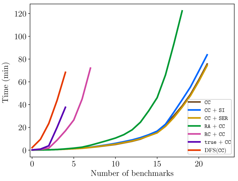
(a) Running time.

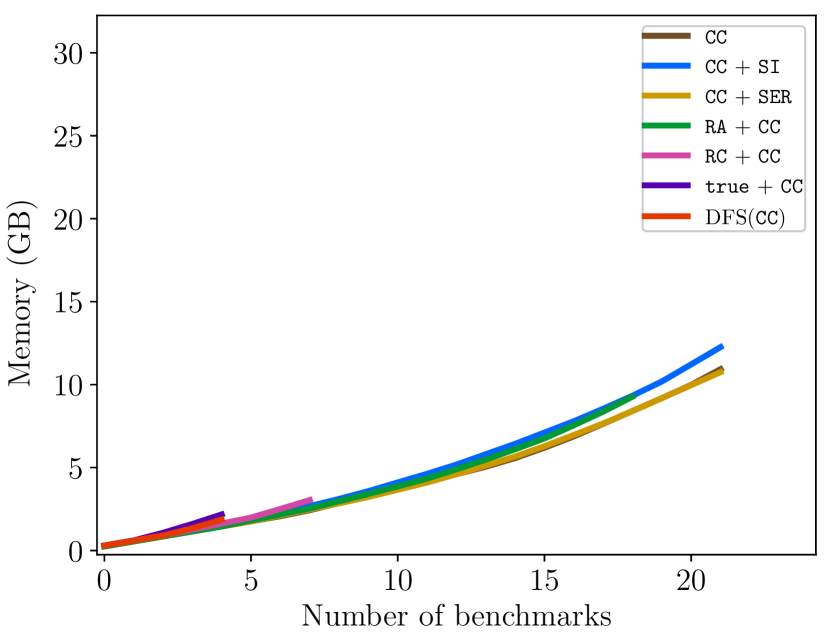
(b) Memory consumption.

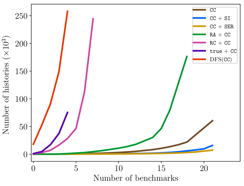
(c) End states.

Figure 14. Cactus plots comparing different algorithms in terms of time, memory, and end states. For readability, we use CC to denote explore-ce under CC, $I_{1}+I_{2}$ stands for $\textsc{explore-ce}^{*}(I_{1},I_{2})$, and true is the trivial isolation level where every history is consistent. Differences between CC, $\textup{{CC}}+\textup{{SI}}$ and $\textup{{CC}}+\textup{{SER}}$ are very small and their graphics overlap. Moreover, $\textsc{DFS}(\textup{{CC}})$ denotes a standard DFS traversal of the semantics defined in Section 2.3. These plots exclude benchmarks that timeout ($30$ mins): $3$ benchmarks for CC, $\langle\textup{{SI}},\textup{{CC}}\rangle$ and $\langle\textup{{SER}},\textup{{CC}}\rangle$ and $6$, $17$, $20$ and $20$ benchmarks timeout for $\langle\textup{{RA}},\textup{{CC}}\rangle$, $\langle\textup{{RC}},\textup{{CC}}\rangle$, $\langle\texttt{true},\textup{{CC}}\rangle$ and $\textsc{DFS}(\textup{{CC}})$ respectively.

To justify the benefits of partial order reduction, we implement a baseline model checking algorithm $\textsc{DFS}(\textup{{CC}})$ that performs a standard DFS traversal of the execution tree w.r.t. the formal semantics defined in Section 2.3 for CC (for fairness, we restrict interleavings so at most one transaction is pending at a time). This baseline algorithm may explore the same history multiple times since it includes no partial order reduction mechanism. In terms of time, $\textsc{DFS}(\textup{{CC}})$ behaves poorly: it timeouts for $20$ out of the $25$ programs and it is less efficient even when it terminates. We consider a timeout of $30$ mins. In comparison the strongly optimal algorithm $\textsc{explore-ce}(\textup{{CC}})$ (under CC) finishes in in $3^{\prime}26^{\prime\prime}$ seconds in average (counting timeouts). $\textsc{DFS}(\textup{{CC}})$ is similiar to $\textsc{explore-ce}(\textup{{CC}})$ in terms of memory consumption. The memory consumption of $\textsc{DFS}(\textup{{CC}})$ is $381$MB in average, compared to $508$MB for $\textsc{explore-ce}(\textup{{CC}})$ (JPF forces a minimum consumption of $256$MB).

To show the benefits of strong optimality, we compare $\textsc{explore-ce}(\textup{{CC}})$ which is strongly optimal with “plain” optimal algorithms $\textsc{explore-ce}^{*}(I_{0},\textup{{CC}})$ for different levels $I_{0}$. As shown in Figure 14(a), $\textsc{explore-ce}(\textup{{CC}})$ is more efficient time-wise than every “plain” optimal algorithm, and the difference in performance grows as $I_{0}$ becomes weaker. In the limit, when $I_{0}$ is the trivial isolation level true where every history is consistent, $\textsc{explore-ce}^{*}(\texttt{true},\textup{{CC}})$ timeouts for $20$ out of the $25$ programs. The average speedup (average of individual speedups) of $\textsc{explore-ce}(\textup{{CC}})$ w.r.t. $\textsc{explore-ce}^{*}(\textup{{RA}},\textup{{CC}})$, $\textsc{explore-ce}^{*}(\textup{{RC}},\textup{{CC}})$ and $\textsc{explore-ce}^{*}(\texttt{true},\textup{{CC}})$ is $3$, $18$ and $15$. respectively (we exclude timeout cases when computing speedups). All algorithms consume around $500$MB of memory in average.

For the SI and SER isolation levels that admit no strongly optimal explore algorithm, we observe that the overhead of $\textsc{explore-ce}^{*}(\textup{{CC}},\textup{{SI}})$ or $\textsc{explore-ce}^{*}(\textup{{CC}},\textup{{SER}})$ relative to $\textsc{explore-ce}(\textup{{CC}})$ is negligible (the corresponding lines in Figure 14 are essentially overlapping). This is due to the fact that the consistency checking algorithms of Biswas and Enea (2019) are polynomial time when the number of sessions is fixed, which makes them fast at least on histories with few sessions.

In our second experiment, we investigate the scalability of explore-ce when increasing the number of sessions. For each $i\in[1,5]$, we consider 5 (independent) client programs for TPC-C and 5 for Wikipedia (10 in total) with $i$ sessions, each session containing 3 transactions. We start with 10 programs with 5 sessions, and remove sessions one by one to obtain programs with fewer sessions. We take CC as isolation level. The plot in Figure 15(a) shows average running time and memory consumption for each number $i\in[1,5]$ of sessions. As expected, increasing the number of sessions is a bottleneck running time wise because the number of histories increases significantly. However, memory consumption does not grow with the same trend, cf. the polynomial space bound.

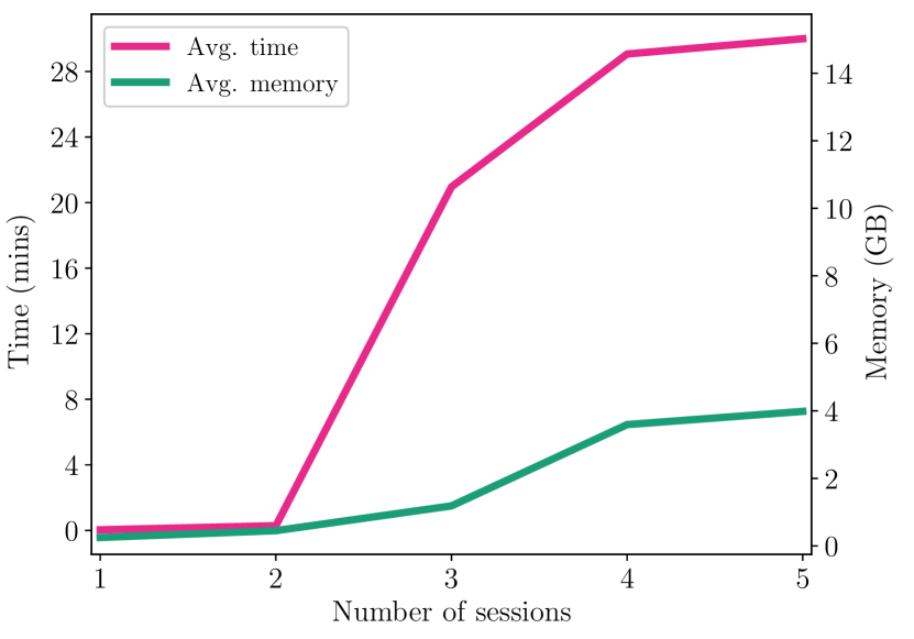
(a) Increasing sessions.

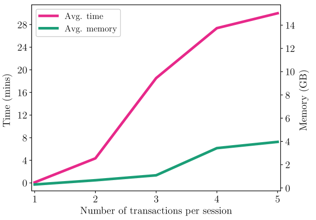
(b) Increasing transactions per session.

Figure 15. Evaluating the scalability of $\textsc{explore-ce}(\textup{{CC}})$ for TPC-C and Wikipedia client programs when increasing their size. These plots include benchmarks that timeout ($30$ mins): $4$, $9$ and $10$ for $3$, $4$ and $5$ sessions respectively in Figure 15(a), and $5$, $8$ and $10$ for $3$, $4$ and $5$ transactions per sessions respectively in Figure 15(b).

Finally, we evaluate the scalability of $\textsc{explore-ce}(\textup{{CC}})$ when increasing the number of transactions per session. We consider 5 (independent) TPC-C client programs and 5 (independent) Wikipedia programs with $3$ sessions and $i$ transactions per session, for each $i\in[1,5]$. Figure 15(b) shows average running time and memory consumption for each number $i\in[1,5]$ of transactions per session. Increasing the number of transactions per session is a bottleneck for the same reasons.

8. Related Work

Checking Correctness of Database-Backed Applications. One line of work is concerned with the logical formalization of isolation levels (X3, 1992; Adya et al., 2000; Berenson et al., 1995; Cerone et al., 2015; Biswas and Enea, 2019). Our work relies on the axiomatic definitions of isolation levels introduced by Biswas and Enea (2019), which have also investigated the problem of checking whether a given history satisfies a certain isolation level. Our SMC algorithms rely on these algorithms to check consistency of a history with a given isolation level.

Another line of work focuses on the problem of finding “anomalies”: behaviors that are not possible under serializability. This is typically done via a static analysis of the application code that builds a static dependency graph that over-approximates the data dependencies in all possible executions of the application (Cerone and Gotsman, 2018; Bernardi and Gotsman, 2016; Fekete et al., 2005; Jorwekar et al., 2007; Warszawski and Bailis, 2017; Gan et al., 2020). Anomalies with respect to a given isolation level then correspond to a particular class of cycles in this graph. Static dependency graphs turn out to be highly imprecise in representing feasible executions, leading to false positives. Another source of false positives is that an anomaly might not be a bug because the application may already be designed to handle the non-serializable behavior (Brutschy et al., 2018; Gan et al., 2020). Recent work has tried to address these issues by using more precise logical encodings of the application (Brutschy et al., 2017, 2018), or by using user-guided heuristics (Gan et al., 2020). Another approach consists of modeling the application logic and the isolation level in first-order logic and relying on SMT solvers to search for anomalies (Kaki et al., 2018; Nagar and Jagannathan, 2018; Ozkan, 2020), or defining specialized reductions to assertion checking (Beillahi et al., 2019b, a). Our approach, based on SMC, does not generate false positives because we systematically enumerate only valid executions of a program which allows to check for user-defined assertions.

Several works have looked at the problem of reasoning about the correctness of applications executing under weak isolation and introducing additional synchronization when necessary (Balegas et al., 2015; Gotsman et al., 2016; Nair et al., 2020; Li et al., 2014). These are based on static analysis or logical proof arguments. The issue of repairing applications is orthogonal to our work.

MonkeyDB (Biswas et al., 2021) is a mock storage system for testing storage-backed applications. While being able to scale to larger code, it has the inherent incompleteness of testing. As opposed to MonkeyDB, our algorithms perform a systematic and complete exploration of executions and can establish correctness at least in some bounded context, and they avoid redundancy, enumerating equivalent executions multiple times. Such guarantees are beyond the scope of MonkeyDB.

Dynamic Partial Order Reduction. Abdulla et al. (2017b) introduced the concept of source sets which provided the first strongly optimal DPOR algorithm for Mazurkiewicz trace equivalence. Other works study DPOR techniques for coarser equivalence relations, e.g., (Abdulla et al., 2019; Agarwal et al., 2021; Aronis et al., 2018; Chalupa et al., 2018; Chatterjee et al., 2019). In all cases, the space complexity is exponential when strong optimality is ensured.

Other works focus on extending DPOR to weak memory models either by targeting a specific memory model (Abdulla et al., 2016, 2017a, 2018; Norris and Demsky, 2013) or by being parametric with respect to an axiomatically-defined memory model (Kokologiannakis et al., 2019; Kokologiannakis and Vafeiadis, 2020; Kokologiannakis et al., 2022). Some of these works can deal with the coarser reads-from equivalence, e.g., (Abdulla et al., 2018; Kokologiannakis et al., 2019; Kokologiannakis and Vafeiadis, 2020; Kokologiannakis et al., 2022). Our algorithms build on the work of Kokologiannakis et al. (2022) which for the first time, proposes a DPOR algorithm which is both strongly optimal and polynomial space. The definitions of database isolation levels are quite different with respect to weak memory models, which makes these previous works not extensible in a direct manner. These definitions include a semantics for transactions which are collections of reads and writes, and this poses new difficult challenges. For instance, reasoning about the completeness and the (strong) optimality of existing DPOR algorithms for shared-memory is agnostic to the scheduler (Next function) while the strong optimality of our explore-ce algorithm relies on the scheduler keeping at most one transaction pending at a time. In addition, unlike TruSt, explore-ce ensures that no swapped events can be swapped again and that the history order $<$ is an extension of ${\color[rgb]{0.5,0,0.5}\mathsf{so}}\cup{\color[rgb]{0,0.5,0}\mathsf{wr}}$. This makes our completeness and optimality proofs radically different. Moreover, even for transactional programs with one access per transaction, where SER and SC are equivalent, TruSt under SC and $\textsc{explore-ce}^{*}(I_{0},\textup{{SER}})$ do not coincide, for any $I_{0}\in\{\textup{{RC}},\textup{{RA}},\textup{{CC}}\}$. In this case, TruSt enumerates only SC-consistent histories at the cost of solving an NP-complete problem at each step while the $\textsc{explore-ce}^{*}$ step cost is polynomial time at the price of not being strongly-optimal. Furthermore, we identify isolation levels (SI and SER) for which it is impossible to ensure both strong optimality and polynomial space bounds with a swapping-based algorithm, a type of question that has not been investigated in previous work.

9. Conclusions

We presented efficient SMC algorithms based on DPOR for transactional programs running under standard isolation levels. These algorithms are instances of a generic schema, called swapping-based algorithms, which is parametrized by an isolation level. Our algorithms are sound and complete, and polynomial space. Additionally, we identified a class of isolation levels, including RC, RA, and CC, for which our algorithms are strongly optimal, and we showed that swapping-based algorithms cannot be strongly optimal for stronger levels SI and SER (but just optimal). For the isolation levels we considered, there is an intriguing coincidence between the existence of a strongly optimal swapping-based algorithm and the complexity of checking if a given history is consistent with that level. Indeed, checking consistency is polynomial time for RC, RA, and CC, and NP-complete for SI and SER. Investigating further the relationship between strong optimality and polynomial-time consistency checks is an interesting direction for future work.

Data availability statement

The implementation is open-source and can be found in (Bouajjani et al., 2023b).

Appendix A Axiomatic levels: Read Committed and Read Atomic.

$\forall x,\ \forall t_{1},t_{2},\ \forall\alpha.\ t_{1}\neq t_{2}\ \land$

${\left\langle{t_{1},\alpha}\right\rangle}\in{\color[rgb]{0,0.5,0}\mathsf{wr}}_{x}\land{t_{2}}\ \mathsf{writes}\ {x}\ \land$

${\left\langle{t_{2},\alpha}\right\rangle}\in{\color[rgb]{0,0.5,0}\mathsf{wr}}\circ{\color[rgb]{0.76953125,0.1171875,0.2265625}\mathsf{po}}$

$\Rightarrow{\left\langle{t_{2},t_{1}}\right\rangle}\in{\color[rgb]{0.703125,0.4453125,0}\mathsf{co}}$

(a) $\mathsf{Read\ Committed}$

$\forall x,\ \forall t_{1},t_{2},\ \forall t_{3}.\ t_{1}\neq t_{2}\ \land$

${\left\langle{t_{1},t_{3}}\right\rangle}\in{\color[rgb]{0,0.5,0}\mathsf{wr}}_{x}\land{t_{2}}\ \mathsf{writes}\ {x}\ \land$

${\left\langle{t_{2},t_{3}}\right\rangle}\in{\color[rgb]{0.5,0,0.5}\mathsf{so}}\cup{\color[rgb]{0,0.5,0}\mathsf{wr}}$

$\Rightarrow{\left\langle{t_{2},t_{1}}\right\rangle}\in{\color[rgb]{0.703125,0.4453125,0}\mathsf{co}}$

(b) $\mathsf{Read\ Atomic}$

Figure A.1. Axioms defining isolations levels. The reflexive and transitive, resp., transitive, closure of a relation $rel$ is denoted by $rel^{*}$, resp., $rel^{+}$. Also, $\circ$ denotes the composition of two relations, i.e., $rel_{1}\circ rel_{2}=\{{\left\langle{a,b}\right\rangle}|\exists c.{\left\langle{a,c}\right\rangle}\in rel_{1}\land{\left\langle{c,b}\right\rangle}\in rel_{2}\}$.

The axioms defined above in Figure A.1 define the homonymous isolation levels Read Atomic (also called Repeatable Read in the literature) and Read Committed.

Appendix B Rules of the operational semantics (Section 2.3).

[spawn]t fresh e fresh P(j) = begin; Body; commit; S  →B(j) = ϵ h,→γ,→B,P ⇒_I h⊕_j ⟨t,{⟨e,begin⟩},∅⟩,→γ[j↦∅],→B[j↦Body; commit],P[j↦S]

[if-true]ψ(→x)[x↦→γ(j)(x): x∈→x] true
→B(j) = if(ψ(→x)) { Instr };B h,→γ,→B, P ⇒_I h,→γ,→B[j↦Instr;B],P

[if-false]ψ(→x)[x↦

References

- (1)
- Abdulla et al. (2017a) Parosh Aziz Abdulla, Stavros Aronis, Mohamed Faouzi Atig, Bengt Jonsson, Carl Leonardsson, and Konstantinos Sagonas. 2017a. Stateless model checking for TSO and PSO. Acta Informatica 54, 8 (2017), 789–818. https://doi.org/10.1007/s00236-016-0275-0
- Abdulla et al. (2017b) Parosh Aziz Abdulla, Stavros Aronis, Bengt Jonsson, and Konstantinos Sagonas. 2017b. Source Sets: A Foundation for Optimal Dynamic Partial Order Reduction. J. ACM 64, 4 (2017), 25:1–25:49. https://doi.org/10.1145/3073408
- Abdulla et al. (2019) Parosh Aziz Abdulla, Mohamed Faouzi Atig, Bengt Jonsson, Magnus Lång, Tuan Phong Ngo, and Konstantinos Sagonas. 2019. Optimal stateless model checking for reads-from equivalence under sequential consistency. Proc. ACM Program. Lang. 3, OOPSLA (2019), 150:1–150:29. https://doi.org/10.1145/3360576
- Abdulla et al. (2016) Parosh Aziz Abdulla, Mohamed Faouzi Atig, Bengt Jonsson, and Carl Leonardsson. 2016. Stateless Model Checking for POWER. In Computer Aided Verification - 28th International Conference, CAV 2016, Toronto, ON, Canada, July 17-23, 2016, Proceedings, Part II (Lecture Notes in Computer Science, Vol. 9780), Swarat Chaudhuri and Azadeh Farzan (Eds.). Springer, 134–156. https://doi.org/10.1007/978-3-319-41540-6_8
- Abdulla et al. (2018) Parosh Aziz Abdulla, Mohamed Faouzi Atig, Bengt Jonsson, and Tuan Phong Ngo. 2018. Optimal stateless model checking under the release-acquire semantics. Proc. ACM Program. Lang. 2, OOPSLA (2018), 135:1–135:29. https://doi.org/10.1145/3276505
- Adya (1999) A. Adya. 1999. Weak Consistency: A Generalized Theory and Optimistic Implementations for Distributed Transactions. Technical Report. USA.
- Adya et al. (2000) Atul Adya, Barbara Liskov, and Patrick E. O’Neil. 2000. Generalized Isolation Level Definitions. In Proceedings of the 16th International Conference on Data Engineering, San Diego, California, USA, February 28 - March 3, 2000, David B. Lomet and Gerhard Weikum (Eds.). IEEE Computer Society, 67–78. https://doi.org/10.1109/ICDE.2000.839388
- Agarwal et al. (2021) Pratyush Agarwal, Krishnendu Chatterjee, Shreya Pathak, Andreas Pavlogiannis, and Viktor Toman. 2021. Stateless Model Checking Under a Reads-Value-From Equivalence. In Computer Aided Verification - 33rd International Conference, CAV 2021, Virtual Event, July 20-23, 2021, Proceedings, Part I (Lecture Notes in Computer Science, Vol. 12759), Alexandra Silva and K. Rustan M. Leino (Eds.). Springer, 341–366. https://doi.org/10.1007/978-3-030-81685-8_16
- Akkoorath and Bieniusa (2016) Deepthi Devaki Akkoorath and Annette Bieniusa. 2016. Antidote: the highly-available geo-replicated database with strongest guarantees. Technical Report. https://pages.lip6.fr/syncfree/attachments/article/59/antidote-white-paper.pdf
- Aronis et al. (2018) Stavros Aronis, Bengt Jonsson, Magnus Lång, and Konstantinos Sagonas. 2018. Optimal Dynamic Partial Order Reduction with Observers. In Tools and Algorithms for the Construction and Analysis of Systems - 24th International Conference, TACAS 2018, Held as Part of the European Joint Conferences on Theory and Practice of Software, ETAPS 2018, Thessaloniki, Greece, April 14-20, 2018, Proceedings, Part II (Lecture Notes in Computer Science, Vol. 10806), Dirk Beyer and Marieke Huisman (Eds.). Springer, 229–248. https://doi.org/10.1007/978-3-319-89963-3_14
- Balegas et al. (2015) Valter Balegas, Sérgio Duarte, Carla Ferreira, Rodrigo Rodrigues, Nuno M. Preguiça, Mahsa Najafzadeh, and Marc Shapiro. 2015. Putting consistency back into eventual consistency. In Proceedings of the Tenth European Conference on Computer Systems, EuroSys 2015, Bordeaux, France, April 21-24, 2015, Laurent Réveillère, Tim Harris, and Maurice Herlihy (Eds.). ACM, 6:1–6:16. https://doi.org/10.1145/2741948.2741972
- Beillahi et al. (2019a) Sidi Mohamed Beillahi, Ahmed Bouajjani, and Constantin Enea. 2019a. Checking Robustness Against Snapshot Isolation. In Computer Aided Verification - 31st International Conference, CAV 2019, New York City, NY, USA, July 15-18, 2019, Proceedings, Part II (Lecture Notes in Computer Science, Vol. 11562), Isil Dillig and Serdar Tasiran (Eds.). Springer, 286–304. https://doi.org/10.1007/978-3-030-25543-5_17
- Beillahi et al. (2019b) Sidi Mohamed Beillahi, Ahmed Bouajjani, and Constantin Enea. 2019b. Robustness Against Transactional Causal Consistency. In 30th International Conference on Concurrency Theory, CONCUR 2019, August 27-30, 2019, Amsterdam, the Netherlands (LIPIcs, Vol. 140), Wan J. Fokkink and Rob van Glabbeek (Eds.). Schloss Dagstuhl - Leibniz-Zentrum für Informatik, 30:1–30:18. https://doi.org/10.4230/LIPIcs.CONCUR.2019.30
- Berenson et al. (1995) Hal Berenson, Philip A. Bernstein, Jim Gray, Jim Melton, Elizabeth J. O’Neil, and Patrick E. O’Neil. 1995. A Critique of ANSI SQL Isolation Levels. In Proceedings of the 1995 ACM SIGMOD International Conference on Management of Data, San Jose, California, USA, May 22-25, 1995, Michael J. Carey and Donovan A. Schneider (Eds.). ACM Press, 1–10. https://doi.org/10.1145/223784.223785
- Bernardi and Gotsman (2016) Giovanni Bernardi and Alexey Gotsman. 2016. Robustness against Consistency Models with Atomic Visibility. In 27th International Conference on Concurrency Theory, CONCUR 2016, August 23-26, 2016, Québec City, Canada (LIPIcs, Vol. 59), Josée Desharnais and Radha Jagadeesan (Eds.). Schloss Dagstuhl - Leibniz-Zentrum für Informatik, 7:1–7:15. https://doi.org/10.4230/LIPIcs.CONCUR.2016.7
- Biswas and Enea (2019) Ranadeep Biswas and Constantin Enea. 2019. On the complexity of checking transactional consistency. Proc. ACM Program. Lang. 3, OOPSLA (2019), 165:1–165:28. https://doi.org/10.1145/3360591
- Biswas et al. (2021) Ranadeep Biswas, Diptanshu Kakwani, Jyothi Vedurada, Constantin Enea, and Akash Lal. 2021. MonkeyDB: effectively testing correctness under weak isolation levels. Proc. ACM Program. Lang. 5, OOPSLA (2021), 1–27. https://doi.org/10.1145/3485546
- Bouajjani et al. (2023a) Ahmed Bouajjani, Constantin Enea, and Enrique Román-Calvo. 2023a. Dynamic Partial Order Reduction for Checking Correctness Against Transaction Isolation Levels. arXiv:2303.12606 [cs.PL]
- Bouajjani et al. (2023b) Ahmed Bouajjani, Constantin Enea, and Enrique Román-Calvo. 2023b. Transactional JPF. https://doi.org/10.5281/zenodo.7824546
- Brain et al. (2017) Martin Brain, James H. Davenport, and Alberto Griggio. 2017. Benchmarking Solvers, SAT-style. In Proceedings of the 2nd International Workshop on Satisfiability Checking and Symbolic Computation co-located with the 42nd International Symposium on Symbolic and Algebraic Computation (ISSAC 2017), Kaiserslautern, Germany, July 29, 2017 (CEUR Workshop Proceedings, Vol. 1974), Matthew England and Vijay Ganesh (Eds.). CEUR-WS.org. http://ceur-ws.org/Vol-1974/RP3.pdf
- Bronson et al. (2013) Nathan Bronson, Zach Amsden, George Cabrera, Prasad Chakka, Peter Dimov, Hui Ding, Jack Ferris, Anthony Giardullo, Sachin Kulkarni, Harry C. Li, Mark Marchukov, Dmitri Petrov, Lovro Puzar, Yee Jiun Song, and Venkateshwaran Venkataramani. 2013. TAO: Facebook’s Distributed Data Store for the Social Graph. In 2013 USENIX Annual Technical Conference, San Jose, CA, USA, June 26-28, 2013, Andrew Birrell and Emin Gün Sirer (Eds.). USENIX Association, 49–60. https://www.usenix.org/conference/atc13/technical-sessions/presentation/bronson
- Brutschy et al. (2017) Lucas Brutschy, Dimitar K. Dimitrov, Peter Müller, and Martin T. Vechev. 2017. Serializability for eventual consistency: criterion, analysis, and applications. In Proceedings of the 44th ACM SIGPLAN Symposium on Principles of Programming Languages, POPL 2017, Paris, France, January 18-20, 2017, Giuseppe Castagna and Andrew D. Gordon (Eds.). ACM, 458–472. https://doi.org/10.1145/3009837.3009895
- Brutschy et al. (2018) Lucas Brutschy, Dimitar K. Dimitrov, Peter Müller, and Martin T. Vechev. 2018. Static serializability analysis for causal consistency. In Proceedings of the 39th ACM SIGPLAN Conference on Programming Language Design and Implementation, PLDI 2018, Philadelphia, PA, USA, June 18-22, 2018, Jeffrey S. Foster and Dan Grossman (Eds.). ACM, 90–104. https://doi.org/10.1145/3192366.3192415
- Cerone et al. (2015) Andrea Cerone, Giovanni Bernardi, and Alexey Gotsman. 2015. A Framework for Transactional Consistency Models with Atomic Visibility. In 26th International Conference on Concurrency Theory, CONCUR 2015, Madrid, Spain, September 1.4, 2015 (LIPIcs, Vol. 42), Luca Aceto and David de Frutos-Escrig (Eds.). Schloss Dagstuhl - Leibniz-Zentrum für Informatik, 58–71. https://doi.org/10.4230/LIPIcs.CONCUR.2015.58
- Cerone and Gotsman (2018) Andrea Cerone and Alexey Gotsman. 2018. Analysing Snapshot Isolation. J. ACM 65, 2 (2018), 11:1–11:41. https://doi.org/10.1145/3152396
- Chalupa et al. (2018) Marek Chalupa, Krishnendu Chatterjee, Andreas Pavlogiannis, Nishant Sinha, and Kapil Vaidya. 2018. Data-centric dynamic partial order reduction. Proc. ACM Program. Lang. 2, POPL (2018), 31:1–31:30. https://doi.org/10.1145/3158119
- Chatterjee et al. (2019) Krishnendu Chatterjee, Andreas Pavlogiannis, and Viktor Toman. 2019. Value-centric dynamic partial order reduction. Proc. ACM Program. Lang. 3, OOPSLA (2019), 124:1–124:29. https://doi.org/10.1145/3360550
- Clarke et al. (1983) Edmund M. Clarke, E. Allen Emerson, and A. Prasad Sistla. 1983. Automatic Verification of Finite State Concurrent Systems Using Temporal Logic Specifications: A Practical Approach. In Conference Record of the Tenth Annual ACM Symposium on Principles of Programming Languages, Austin, Texas, USA, January 1983, John R. Wright, Larry Landweber, Alan J. Demers, and Tim Teitelbaum (Eds.). ACM Press, 117–126. https://doi.org/10.1145/567067.567080
- Clarke et al. (1999) Edmund M. Clarke, Orna Grumberg, Marius Minea, and Doron A. Peled. 1999. State Space Reduction Using Partial Order Techniques. Int. J. Softw. Tools Technol. Transf. 2, 3 (1999), 279–287. https://doi.org/10.1007/s100090050035
- DeCandia et al. (2007) Giuseppe DeCandia, Deniz Hastorun, Madan Jampani, Gunavardhan Kakulapati, Avinash Lakshman, Alex Pilchin, Swaminathan Sivasubramanian, Peter Vosshall, and Werner Vogels. 2007. Dynamo: amazon’s highly available key-value store. In Proceedings of the 21st ACM Symposium on Operating Systems Principles 2007, SOSP 2007, Stevenson, Washington, USA, October 14-17, 2007, Thomas C. Bressoud and M. Frans Kaashoek (Eds.). ACM, 205–220. https://doi.org/10.1145/1294261.1294281
- Difallah et al. (2013) Djellel Eddine Difallah, Andrew Pavlo, Carlo Curino, and Philippe Cudré-Mauroux. 2013. OLTP-Bench: An Extensible Testbed for Benchmarking Relational Databases. Proc. VLDB Endow. 7, 4 (2013), 277–288. https://doi.org/10.14778/2732240.2732246
- Fekete et al. (2005) Alan D. Fekete, Dimitrios Liarokapis, Elizabeth J. O’Neil, Patrick E. O’Neil, and Dennis E. Shasha. 2005. Making snapshot isolation serializable. ACM Trans. Database Syst. 30, 2 (2005), 492–528. https://doi.org/10.1145/1071610.1071615
- Flanagan and Godefroid (2005) Cormac Flanagan and Patrice Godefroid. 2005. Dynamic partial-order reduction for model checking software. In Proceedings of the 32nd ACM SIGPLAN-SIGACT Symposium on Principles of Programming Languages, POPL 2005, Long Beach, California, USA, January 12-14, 2005, Jens Palsberg and Martín Abadi (Eds.). ACM, 110–121. https://doi.org/10.1145/1040305.1040315
- Gan et al. (2020) Yifan Gan, Xueyuan Ren, Drew Ripberger, Spyros Blanas, and Yang Wang. 2020. IsoDiff: Debugging Anomalies Caused by Weak Isolation. Proc. VLDB Endow. 13, 12 (July 2020), 27732786. https://doi.org/10.14778/3407790.3407860
- Godefroid (1996) Patrice Godefroid. 1996. Partial-Order Methods for the Verification of Concurrent Systems - An Approach to the State-Explosion Problem. Lecture Notes in Computer Science, Vol. 1032. Springer. https://doi.org/10.1007/3-540-60761-7
- Godefroid (1997) Patrice Godefroid. 1997. Model Checking for Programming Languages using Verisoft. In Conference Record of POPL’97: The 24th ACM SIGPLAN-SIGACT Symposium on Principles of Programming Languages, Papers Presented at the Symposium, Paris, France, 15-17 January 1997, Peter Lee, Fritz Henglein, and Neil D. Jones (Eds.). ACM Press, 174–186. https://doi.org/10.1145/263699.263717
- Gotsman et al. (2016) Alexey Gotsman, Hongseok Yang, Carla Ferreira, Mahsa Najafzadeh, and Marc Shapiro. 2016. ’Cause I’m strong enough: reasoning about consistency choices in distributed systems. In Proceedings of the 43rd Annual ACM SIGPLAN-SIGACT Symposium on Principles of Programming Languages, POPL 2016, St. Petersburg, FL, USA, January 20 - 22, 2016, Rastislav Bodík and Rupak Majumdar (Eds.). ACM, 371–384. https://doi.org/10.1145/2837614.2837625
- Jorwekar et al. (2007) Sudhir Jorwekar, Alan D. Fekete, Krithi Ramamritham, and S. Sudarshan. 2007. Automating the Detection of Snapshot Isolation Anomalies. In Proceedings of the 33rd International Conference on Very Large Data Bases, University of Vienna, Austria, September 23-27, 2007, Christoph Koch, Johannes Gehrke, Minos N. Garofalakis, Divesh Srivastava, Karl Aberer, Anand Deshpande, Daniela Florescu, Chee Yong Chan, Venkatesh Ganti, Carl-Christian Kanne, Wolfgang Klas, and Erich J. Neuhold (Eds.). ACM, 1263–1274. http://www.vldb.org/conf/2007/papers/industrial/p1263-jorwekar.pdf
- Kaki et al. (2018) Gowtham Kaki, Kapil Earanky, K. C. Sivaramakrishnan, and Suresh Jagannathan. 2018. Safe replication through bounded concurrency verification. Proc. ACM Program. Lang. 2, OOPSLA (2018), 164:1–164:27. https://doi.org/10.1145/3276534
- Kokologiannakis et al. (2022) Michalis Kokologiannakis, Iason Marmanis, Vladimir Gladstein, and Viktor Vafeiadis. 2022. Truly stateless, optimal dynamic partial order reduction. Proc. ACM Program. Lang. 6, POPL (2022), 1–28. https://doi.org/10.1145/3498711
- Kokologiannakis et al. (2019) Michalis Kokologiannakis, Azalea Raad, and Viktor Vafeiadis. 2019. Model checking for weakly consistent libraries. In Proceedings of the 40th ACM SIGPLAN Conference on Programming Language Design and Implementation, PLDI 2019, Phoenix, AZ, USA, June 22-26, 2019, Kathryn S. McKinley and Kathleen Fisher (Eds.). ACM, 96–110. https://doi.org/10.1145/3314221.3314609
- Kokologiannakis and Vafeiadis (2020) Michalis Kokologiannakis and Viktor Vafeiadis. 2020. HMC: Model Checking for Hardware Memory Models. In ASPLOS ’20: Architectural Support for Programming Languages and Operating Systems, Lausanne, Switzerland, March 16-20, 2020, James R. Larus, Luis Ceze, and Karin Strauss (Eds.). ACM, 1157–1171. https://doi.org/10.1145/3373376.3378480
- Lamport (1978) Leslie Lamport. 1978. Time, Clocks, and the Ordering of Events in a Distributed System. Commun. ACM 21, 7 (1978), 558–565. https://doi.org/10.1145/359545.359563
- Li et al. (2014) Cheng Li, João Leitão, Allen Clement, Nuno M. Preguiça, Rodrigo Rodrigues, and Viktor Vafeiadis. 2014. Automating the Choice of Consistency Levels in Replicated Systems. In 2014 USENIX Annual Technical Conference, USENIX ATC ’14, Philadelphia, PA, USA, June 19-20, 2014, Garth Gibson and Nickolai Zeldovich (Eds.). USENIX Association, 281–292. https://www.usenix.org/conference/atc14/technical-sessions/presentation/li_cheng_2
- Lloyd et al. (2011) Wyatt Lloyd, Michael J. Freedman, Michael Kaminsky, and David G. Andersen. 2011. Don’t settle for eventual: scalable causal consistency for wide-area storage with COPS. In Proceedings of the 23rd ACM Symposium on Operating Systems Principles 2011, SOSP 2011, Cascais, Portugal, October 23-26, 2011, Ted Wobber and Peter Druschel (Eds.). ACM, 401–416. https://doi.org/10.1145/2043556.2043593
- Mazurkiewicz (1986) Antoni W. Mazurkiewicz. 1986. Trace Theory. In Petri Nets: Central Models and Their Properties, Advances in Petri Nets 1986, Part II, Proceedings of an Advanced Course, Bad Honnef, Germany, 8-19 September 1986 (Lecture Notes in Computer Science, Vol. 255), Wilfried Brauer, Wolfgang Reisig, and Grzegorz Rozenberg (Eds.). Springer, 279–324. https://doi.org/10.1007/3-540-17906-2_30
- Nagar and Jagannathan (2018) Kartik Nagar and Suresh Jagannathan. 2018. Automated Detection of Serializability Violations Under Weak Consistency. In 29th International Conference on Concurrency Theory, CONCUR 2018, September 4-7, 2018, Beijing, China (LIPIcs, Vol. 118), Sven Schewe and Lijun Zhang (Eds.). Schloss Dagstuhl - Leibniz-Zentrum für Informatik, 41:1–41:18. https://doi.org/10.4230/LIPIcs.CONCUR.2018.41
- Nair et al. (2020) Sreeja S. Nair, Gustavo Petri, and Marc Shapiro. 2020. Proving the Safety of Highly-Available Distributed Objects. In Programming Languages and Systems - 29th European Symposium on Programming, ESOP 2020, Held as Part of the European Joint Conferences on Theory and Practice of Software, ETAPS 2020, Dublin, Ireland, April 25-30, 2020, Proceedings (Lecture Notes in Computer Science, Vol. 12075), Peter Müller (Ed.). Springer, 544–571. https://doi.org/10.1007/978-3-030-44914-8_20
- Norris and Demsky (2013) Brian Norris and Brian Demsky. 2013. CDSchecker: checking concurrent data structures written with C/C++ atomics. In Proceedings of the 2013 ACM SIGPLAN International Conference on Object Oriented Programming Systems Languages & Applications, OOPSLA 2013, part of SPLASH 2013, Indianapolis, IN, USA, October 26-31, 2013, Antony L. Hosking, Patrick Th. Eugster, and Cristina V. Lopes (Eds.). ACM, 131–150. https://doi.org/10.1145/2509136.2509514
- Ozkan (2020) Burcu Kulahcioglu Ozkan. 2020. Verifying Weakly Consistent Transactional Programs Using Symbolic Execution. In Networked Systems - 8th International Conference, NETYS 2020, Marrakech, Morocco, June 3-5, 2020, Proceedings (Lecture Notes in Computer Science, Vol. 12129), Chryssis Georgiou and Rupak Majumdar (Eds.). Springer, 261–278. https://doi.org/10.1007/978-3-030-67087-0_17
- Papadimitriou (1979) Christos H. Papadimitriou. 1979. The serializability of concurrent database updates. J. ACM 26, 4 (1979), 631–653. https://doi.org/10.1145/322154.322158
- Pavlo (2017) Andrew Pavlo. 2017. What Are We Doing With Our Lives? Nobody Cares About Our Concurrency Control Research. In Proceedings of the 2017 ACM International Conference on Management of Data (Chicago, Illinois, USA) (SIGMOD ’17). Association for Computing Machinery, New York, NY, USA, 3. https://doi.org/10.1145/3035918.3056096
- Paz (2018) Jos Rolando Guay Paz. 2018. Microsoft Azure Cosmos DB Revealed: A Multi-Modal Database Designed for the Cloud (1st ed.). Apress, USA.
- Peled (1993) Doron A. Peled. 1993. All from One, One for All: on Model Checking Using Representatives. In Computer Aided Verification, 5th International Conference, CAV ’93, Elounda, Greece, June 28 - July 1, 1993, Proceedings (Lecture Notes in Computer Science, Vol. 697), Costas Courcoubetis (Ed.). Springer, 409–423. https://doi.org/10.1007/3-540-56922-7_34
- Queille and Sifakis (1982) Jean-Pierre Queille and Joseph Sifakis. 1982. Specification and verification of concurrent systems in CESAR. In International Symposium on Programming, 5th Colloquium, Torino, Italy, April 6-8, 1982, Proceedings (Lecture Notes in Computer Science, Vol. 137), Mariangiola Dezani-Ciancaglini and Ugo Montanari (Eds.). Springer, 337–351. https://doi.org/10.1007/3-540-11494-7_22
- Rahmani et al. (2019) Kia Rahmani, Kartik Nagar, Benjamin Delaware, and Suresh Jagannathan. 2019. CLOTHO: directed test generation for weakly consistent database systems. Proc. ACM Program. Lang. 3, OOPSLA (2019), 117:1–117:28. https://doi.org/10.1145/3360543
- Sivaramakrishnan et al. (2015) K. C. Sivaramakrishnan, Gowtham Kaki, and Suresh Jagannathan. 2015. Declarative programming over eventually consistent data stores. In Proceedings of the 36th ACM SIGPLAN Conference on Programming Language Design and Implementation, Portland, OR, USA, June 15-17, 2015, David Grove and Stephen M. Blackburn (Eds.). ACM, 413–424. https://doi.org/10.1145/2737924.2737981
- TPC (2010) TPC. 2010. . Technical Report. Transaction Processing Performance Council. http://www.tpc.org/tpc_documents_current_versions/pdf/tpc-c_v5.11.0.pdf
- Valmari (1989) Antti Valmari. 1989. Stubborn sets for reduced state space generation. In Advances in Petri Nets 1990 [10th International Conference on Applications and Theory of Petri Nets, Bonn, Germany, June 1989, Proceedings] (Lecture Notes in Computer Science, Vol. 483), Grzegorz Rozenberg (Ed.). Springer, 491–515. https://doi.org/10.1007/3-540-53863-1_36
- Visser et al. (2004) Willem Visser, Corina S. Pasareanu, and Sarfraz Khurshid. 2004. Test input generation with java PathFinder. In Proceedings of the ACM/SIGSOFT International Symposium on Software Testing and Analysis, ISSTA 2004, Boston, Massachusetts, USA, July 11-14, 2004, George S. Avrunin and Gregg Rothermel (Eds.). ACM, 97–107. https://doi.org/10.1145/1007512.1007526
- Warszawski and Bailis (2017) Todd Warszawski and Peter Bailis. 2017. ACIDRain: Concurrency-Related Attacks on Database-Backed Web Applications. In Proceedings of the 2017 ACM International Conference on Management of Data (Chicago, Illinois, USA) (SIGMOD ’17). Association for Computing Machinery, New York, NY, USA, 520. https://doi.org/10.1145/3035918.3064037
- X3 (1992) ANSI X3. 1992. 135-1992. American National Standard for Information Systems-Database Language-SQL. Technical Report.