Estimation of quadrature errors for layer potentials evaluated near surfaces with spherical topology

Abstract

Numerical simulations with rigid particles, drops or vesicles constitute some examples that involve 3D objects with spherical topology. When the numerical method is based on boundary integral equations, the error in using a regular quadrature rule to approximate the layer potentials that appear in the formulation will increase rapidly as the evaluation point approaches the surface and the integrand becomes sharply peaked. To determine when the accuracy becomes insufficient, and a more costly special quadrature method should be used, error estimates are needed. In this paper we present quadrature error estimates for layer potentials evaluated near surfaces of genus 0, parametrized using a polar and an azimuthal angle, discretized by a combination of the Gauss-Legendre and the trapezoidal quadrature rules. The error estimates involve no unknown coefficients, but complex valued roots of a specified distance function. The evaluation of the error estimates in general requires a one dimensional local root-finding procedure, but for specific geometries we obtain analytical results. Based on these explicit solutions, we derive simplified error estimates for layer potentials evaluated near spheres; these simple formulas depend only on the distance from the surface, the radius of the sphere and the number of discretization points. The usefulness of these error estimates is illustrated with numerical examples.

1 Introduction

We consider a generic layer potential over a regular surface $S\subset\mathbb{R}^{3}$,

$$u(\bm{x})=\int_{S}\frac{k\left(\bm{x},\bm{y}\right)\sigma(\bm{y})}{\mathinner{\!\left\lVert\bm{y}-\bm{x}\right\rVert}^{2p}}\operatorname{d\!}S(\bm{y}),$$ (1)

where $2p\in{\mathbb{Z}}^{+}$ and the evaluation (or target) point $\bm{x}\in\mathbb{R}^{3}$ is allowed to be close to, but not on, $S$. The functions $k\left(\bm{x},\bm{y}\right)$ and $\sigma(\bm{y})$ as well as $S$ are assumed to be smooth. When $\bm{x}$ is close to $S$, the integrand will be peaked around the point on $S$ closest to $\bm{x}$, implying that, while the integral is well defined analytically, it is difficult to resolve well numerically.

In paper AFKLINTEBERG20221 , we derived estimates for the numerical errors that result when applying quadrature rules to such layer potentials. Specifically, we considered the panel based Gauss-Legendre quadrature rule and the global trapezoidal rule. The estimates that was derived have no unknown coefficients and can be efficiently evaluated given the discretization of the surface. The evaluation involves a local one-dimensional root finding procedure. In numerical experiments, we have found the estimates to be both sufficiently precise and computationally cheap to be practically useful. This means that they can be used to determine when the regular quadrature is insufficient for a required accuracy, and hence when a more costly special quadrature method must be invoked. In deriving these estimates, we assumed that the local (for Gauss-Legendre) or global (for trapezoidal rule) surface parametrization is such that the map between the parameter space and the surface coordinates is one-to-one.

For surfaces of genus $0$, topologically equivalent to a sphere, it is quite common to use a global parametrization in two angles, i.e. spherical coordinates. At the poles of such a parametrization, the parameter to surface coordinate map is not one-to-one. Here, the derivative of the surface coordinate with respect to the azimuth angle vanish, and with it, the surface area element. For such parametrizations, the previously derived error estimates cannot be directly used for all evaluation points $\bm{x}$.

It is quite common in applications of boundary integral equations to discretize surfaces with parametrizations based on spherical coordinates, and to that attach a Gaussian grid, i.e. a discretization with a Gauss-Legendre quadrature rule in the polar angle (or a mapping of the polar angle) and the trapezoidal rule in the periodic azimuthal angle. This has been used for simulations of Stokes flow with solid particles in e.g. AfKlinteberg2016qbx ; Corona2017504 , and with drops and vesicles Sorgentone2018167 ; Sorgentone2022 ; Rahimian2015766 ; Veerapaneni2016278 . In the latter case, the deformable shapes are represented by spherical harmonics expansions.

In this paper, we consider the case of a general smooth surface of genus $0$, parametrized using a polar and an azimuthal angle, discretized by a combination of the Gauss-Legendre quadrature rule and the trapezoidal rule as described above. Before we introduce the contributions of this paper, we will briefly describe the derivations of the estimates in paper AFKLINTEBERG20221 , and the previous results that enabled that work.

Consider the following simple integrals

$$\int_{E}\frac{1}{\left((t-a)^{2}+b^{2}\right)^{p}}\,dt=\int_{E}\frac{1}{\left(t-z_{0}\right)^{p}\left(t-\bar{z}_{0}\right)^{p}}\,dt,$$ (2)

with $z_{0}=a+ib$, $a,b\in\mathbb{R}$, $b>0$, $p\in{\mathbb{Z}}^{+}$, and

$$\int_{E}\frac{1}{\left(t-z_{0}\right)^{p}}\,dt,\quad z_{0}=a+ib,\quad a,b\in\mathbb{R},b\neq 0,p\in{\mathbb{Z}}^{+},$$ (3)

over a basic interval $E$, e.g. $[-1,1]$ for Gauss-Legendre and $[0,2\pi)$ for the trapezoidal rule. If $b$ is small the integrands have two poles/one pole close to the integration interval along the real axis. The theory of Donaldson and Elliott Donaldson1972 defines the quadrature error as a contour integral in the complex plane over the integrand multiplied with a so-called remainder function, that depends on the quadrature rule. Elliott et al. Elliott2008 derived error estimates for the error in the approximation of (2) with an $n$-point Gauss-Legendre quadrature rule. To estimate the contour integral, they used residue calculus for $p=1$ and branch cuts for $0<p<1$. In AfKlinteberg2016quad , af Klinteberg and Tornberg derived error estimates for both (2) and (3) for the Gauss-Legendre quadrature rule, for any $p\in{\mathbb{Z}}^{+}$. Corresponding results were derived also for the trapezoidal rule, but for integration over the unit circle. Previous studies on the trapezoidal rule include the survey by Trefethen and Weideman Trefethen2014 , and the error bound provided by Barnett in Barnett2014 for the quadrature error in evaluating the harmonic double layer potential.

In AfKlinteberg2018 , a key step was taken to accurately estimate the quadrature errors for the Gauss-Legendre quadrature rule in the approximation of layer potentials in 2D, written in complex form. Introducing a parametrization of a smooth curve segment, $\gamma(t)\in\mathbb{C}$, a typical form of an integral to evaluate is

$$\int_{E}\frac{f(t)\,\gamma^{\prime}(t)}{(\gamma(t)-z_{0})^{p}}\,dt.$$ (4)

As compared to the estimates for the simple complex integral (3) above, the estimates derived for this integral require the knowledge of $t_{0}\in\mathbb{C}$ such that $\gamma(t_{0})=z_{0}$. In practice, given the Gauss-Legendre points used to discretize the panel, a numerical procedure is used to compute $t_{0}$. Note that not all layer potentials in 2D can be written in this form. Using the same techniques, remarkably accurate error estimates were derived also for layer potentials for the Helmholtz and Stokes equations, in AfKlinteberg2018 and Palsson2019 , respectively.

Now, let $S$ in (1) be a curve $\Gamma\in\mathbb{R}^{2}$, $\Gamma=\gamma(E)$, $E\subset\mathbb{R}$. We can then write the layer potential in (1) in the equivalent form

$$u(\bm{x})=\int_{E}\frac{k\left(\bm{x},\bm{\gamma}(t)\right)\sigma(\bm{\gamma}(t))}{\mathinner{\!\left\lVert\bm{\gamma}(t)-\bm{x}\right\rVert}^{2p}}\mathinner{\!\left\lVert\bm{\gamma}^{\prime}(t)\right\rVert}\operatorname{d\!}t=\int_{E}\frac{f(t)\operatorname{d\!}t}{\mathinner{\!\left\lVert\bm{\gamma}(t)-\bm{x}\right\rVert}^{2p}}.$$ (5)

In the last step all the components that are assumed to be smooth have been collected in the function $f(t)$, which has an implicit dependence on $\bm{x}$. The location of the poles are in this case given by each $t_{0}\in\mathbb{C}$ such that the denominator is zero. In AFKLINTEBERG20221 , error estimates were derived for such integrals, both for the Gauss-Legendre and the trapezoidal quadrature rules. To evaluate these estimates, the pair of the complex conjugate roots $\{t_{0},\bar{t_{0}}\}$ closest to integration interval is needed, and is in practice found through a numerical root-finding procedure. The estimates will be stated in Section 3.

A key observation in AFKLINTEBERG20221 was that the error estimates for the numerical approximation of (5) can be derived the same way for $\Gamma\in\mathbb{R}^{d}$, $d=2,3$. The only difference is that $R^{2}(t,x)=\mathinner{\!\left\lVert\bm{\gamma}(t)-\bm{x}\right\rVert}^{2}$ will have three additive terms instead of two. Starting with the curve estimates in $\mathbb{R}^{3}$, error estimates for the prototype layer potential (1) were derived.

With $S$ a two-dimensional surface in $\mathbb{R}^{3}$, parametrized by $\bm{\gamma}\mathrel{\mathop{\ordinarycolon}}E\rightarrow\mathbb{R}^{3}$, $E=\left\{E_{1}\times E_{2}\right\}\subset\mathbb{R}^{2}$, (1) takes the form

$$u(\bm{x})=\iint_{E}\frac{k\left(\bm{x},\bm{\gamma}(t,\varphi)\right)\sigma(\bm{\gamma}(t,\varphi))}{\mathinner{\!\left\lVert\bm{\gamma}(t,\varphi)-\bm{x}\right\rVert}^{2p}}\mathinner{\!\left\lVert\mathinner{\dfrac{\partial{}\bm{\gamma}}{\partial{t}}}\times\mathinner{\dfrac{\partial{}\bm{\gamma}}{\partial{\varphi}}}\right\rVert}\operatorname{d\!}\varphi\operatorname{d\!}t=\iint_{E}\frac{f(t,\varphi)\operatorname{d\!}\varphi\operatorname{d\!}t}{\mathinner{\!\left\lVert\bm{\gamma}(t,\varphi)-\bm{x}\right\rVert}^{2p}}.$$ (6)

All the components that are assumed to be smooth have here been collected in $f(t,\varphi)$ which depends implicitly on $\bm{x}$. In AFKLINTEBERG20221 error estimates were derived for the numerical approximation of (6) by composite Gauss-Legendre quadrature or global trapezoidal quadrature. Numerical examples were shown with tensor product quadrature rules based on Gauss-Legendre quadrature for surface discretizations of quadrilateral patches, and the tensor product trapezoidal rule for global discretizations.

2 Contributions and outline

In this paper, we will discuss the generalization of the results of paper AFKLINTEBERG20221 to the case of smooth surfaces topologically equivalent to a sphere, parametrized by $\bm{\gamma}^{\circ}\mathrel{\mathop{\ordinarycolon}}U\rightarrow\mathbb{R}^{3}$, where $U=\left\{(\theta,\varphi)\in[0,\pi]\times[0,2\pi)\right\}$.

A generic such surface can be represented by

$$\gamma^{\circ}(\theta,\varphi)=\sum_{\ell=0}^{\infty}\sum_{m=-\ell}^{\ell}\bm{C}_{\ell}^{m}Y_{\ell}^{m}(\theta,\varphi),$$ (7)

where $\bm{C}_{\ell}^{m}\in\mathbb{C}^{3}$ and $Y_{\ell}^{m}(\theta,\varphi)$ is the spherical harmonic function of degree $\ell$ and order $m$.

The surface $\gamma(t,\varphi)$ in (6) can then be defined as

$$\gamma(t,\varphi)=\gamma^{\circ}(\theta(t),\varphi),$$ (8)

where $t\in[-1,1]$ and $\varphi\in[0,2\pi)$. With this parametrization, we can naturally discretize the integral using a $n_{t}$-point Gauss-Legendre quadrature rule in the $t$ coordinate, and a $n_{\varphi}$ point trapezoidal rule in the periodic $\varphi$ coordinate. We will consider two different maps $\theta(t)\mathrel{\mathop{\ordinarycolon}}[-1,1]\rightarrow[0,\pi]$: a simple linear scaling

$$\theta(t)=(t+1)\pi/2,$$ (9)

and a non-linear one

$$\theta(t)=\cos^{-1}(-t)=\pi-\cos^{-1}(t).$$ (10)

The inverse mappings are $t(\theta)=-1+2\theta/\pi$ and $t(\theta)=-\cos(\theta)$, respectively. With both mappings, $t=-1$ corresponds to $\theta=0$.

In section 3, we introduce the error estimates derived in AFKLINTEBERG20221 for the integral over a curve in $\mathbb{R}^{2}$ or $\mathbb{R}^{3}$ (5). In section 4 we then introduce the extension to a surface of genus 0 in $\mathbb{R}^{3}$ for our specific discretizations, based on what was done in paper AFKLINTEBERG20221 . In section 5 we derive analytical results for axisymmetric surfaces. We also show how, based on the explicit knowledge of the roots, it is possible to derive simplified error estimates for layer potentials evaluated near spheres. In section 6, we discuss how to numerically evaluate the estimates for a general surface with spherical topology, and in section 7 we show how the error estimates perform on different numerical examples.

3 Quadrature error estimates for curves in $\mathbb{R}^{2}$ and $\mathbb{R}^{3}$

Let us introduce the base interval $E$, which for the Gauss-Legendre quadrature will be $[-1,1]$ and for the trapezoidal rule $[0,2\pi)$. Consider an integral over such a base interval

$$\mathcal{I}[g]=\int_{E}g(t)\,dt,$$ (11)

and an $n$-point quadrature rule with quadrature nodes $\{t_{\ell}\}_{\ell=1}^{n}$ and corresponding quadrature weights $\{w_{\ell}\}_{\ell=1}^{n}$ to approximate it,

$$Q_{n}[g]=\sum_{\ell=1}^{n}g(t_{\ell})w_{\ell}.$$ (12)

The error

$$E_{n}[g]=\mathcal{I}[g]-Q_{n}[g],$$ (13)

as a function of $n$ will depend on the function $g$ and the specific quadrature rule. We will consider closed curves for the trapezoidal rule and open curves (segments) with the Gauss-Legendre quadrature rule.

We now introduce the squared distance function for a curve in $\mathbb{R}^{d}$ ($d=2$ or $3$), to an evaluation point $\bm{x}\in\mathbb{R}^{d}$,

$$R^{2}(t,\bm{x})\coloneqq\mathinner{\!\left\lVert\bm{\gamma}(t)-\bm{x}\right\rVert}^{2}=\sum_{i=1}^{d}(\gamma_{i}(t)-x_{i})^{2}.$$ (14)

We will later evaluate this function also for $t\in\mathbb{C}$, in which case we will use the right most expression. This expression can then evaluate as a complex number, and will no longer be a norm. Our integral of interest (5) can be written in the form

$$\mathcal{I}[\Theta_{p}](\bm{x})=\int_{E}\Theta_{p}(t,\bm{x})\operatorname{d\!}t,\qquad\Theta_{p}(t,\bm{x})=\frac{f(t)}{\left(R^{2}(t,\bm{x})\right)^{p}},$$ (15)

and we want to estimate $\operatorname{E}_{n}[\Theta_{p}](\bm{x})$.

As $\bm{x}$ is not on $\bm{\gamma}(t)$, we have $R^{2}(t,\bm{x})>0$ for $t\in E$. There will however be complex conjugate pairs of roots to $R^{2}(t,\bm{x})$, since $R^{2}(t,\bm{x})$ is real for real $t$. Let $\left\{t_{0},\overline{t}_{0}\right\}$ be the pair closest to $E$, s.t.

$$R^{2}(t_{0},\bm{x})=R^{2}(\overline{t}_{0},\bm{x})=0.$$ (16)

Under the assumption that $f$ is smooth, the region of analyticity of $\Theta_{p}(t,\bm{x})$ is bounded by these roots. We will henceforth refer to them both as roots (of $R^{2}$) and singularities (of the integrand). They are in most applications not known a priori, but can be found numerically for a given target point $\bm{x}$ (see section 6.2).

The quadrature error $\operatorname{E}_{n}[\Theta_{p}](\bm{x})$ can, following Donaldson and Elliott Donaldson1972 , be written as a contour integral in the complex plane over the integrand $\Theta_{p}(t,\bm{x})$ multiplied with a so-called remainder function, that depends on the quadrature rule. If $p$ is an integer, $t_{0}$ and $\bar{t_{0}}$ are $p$th order poles of the integrand. If $p$ is a half-integer, the integrand has branch points at these singularities.

An important step in the derivation leading up to estimates of the quadrature error in AFKLINTEBERG20221 , is to divide and multiply the integrand with the factor $t-w$, where $w\in\mathbb{C}$ is the singularity at the branch begin considered. This yields the singularity $(t-w)^{-1}$ to consider in the complex plane, and introduces what is denoted the geometry factor.

The geometry factor $G$ is, for an evaluation point $\bm{x}\in\mathbb{R}^{d}$ and $w\in\mathbb{C}$ a root of $R^{2}$, defined as

$$G(w,\bm{x})=\lim_{t\to w}\frac{t-w}{R^{2}(t,\bm{x})}=\left(2\left(\bm{\gamma}(w)-\bm{x}\right)\cdot\bm{\gamma}^{\prime}(w)\right)^{-1}.$$ (17)

With these definitions, we are ready to state the error estimates from AFKLINTEBERG20221 , for both the trapezoidal rule and the Gauss-Legendre quadrature rule.

Error estimate 1 (Trapezoidal rule).

Consider the integral in (15) for an evaluation point $\bm{x}\in\mathbb{R}^{d}$, with $2p\in{\mathbb{Z}}^{+}$, where $\gamma(E)$ is the parametrization of a smooth closed curve in $\mathbb{R}^{d}$ where $d=2$ or $3$. The integrand is assumed to be periodic in $t$ over the integration interval $E=[0,2\pi)$. The error in approximating the integral with the $n$-point trapezoidal rule can in the limit $n\rightarrow\infty$ be estimated as

$$\mathinner{\!\left\lvert\operatorname{E}_{n}[\Theta_{p}](\bm{x})\right\rvert}\approx\frac{4\pi n^{p-1}}{\Gamma(p)}\mathinner{\!\left\lvert f(t_{0})\right\rvert}\mathinner{\!\left\lvert G(t_{0},\bm{x})\right\rvert}^{p}e^{-n\mathinner{\!\left\lvert\operatorname{Im}{t_{0}}\right\rvert}}.$$ (18)

Here, $\Gamma(p)$ the gamma function, and the geometry factor $G$ is defined in (17). The squared distance function is defined in (14), and $\left\{t_{0},\overline{t}_{0}\right\}$ is the pair of complex conjugate roots of this $R^{2}(t,\bm{x})$ closest to the integration interval $E$.

Error estimate 2 (Gauss-Legendre rule).

Consider the integral in (15) for an evaluation point $\bm{x}\in\mathbb{R}^{d}$, with $2p\in{\mathbb{Z}}^{+}$, where $\gamma(E)$ is the parametrization of a smooth closed curve in $\mathbb{R}^{d}$ $d=2$ or $3$, with $E=[-1,1]$. The error in approximating the integral with the $n$-point Gauss-Legendre rule can in the limit $n\rightarrow\infty$ be estimated as

$$\mathinner{\!\left\lvert\operatorname{E}_{n}[\Theta_{p}](\bm{x})\right\rvert}\approx\frac{4\pi}{\Gamma(p)}(2n+1)^{p-1}\mathinner{\!\left\lvert f(t_{0})\right\rvert}\mathinner{\!\left\lvert G(t_{0},\bm{x})\right\rvert}^{p}\frac{\mathinner{\!\left\lvert\sqrt{t_{0}^{2}-1}\right\rvert}^{1-p}}{\mathinner{\!\left\lvert t_{0}+\sqrt{t_{0}^{2}-1}\right\rvert}^{2n+1}},$$ (19)

where $\sqrt{z^{2}-1}$ is defined as $\sqrt{z+1}\sqrt{z-1}$ with $-\pi<\arg(z\pm 1)\leq\pi$. Here, $\Gamma(p)$ the gamma function, the geometry factor $G$ is defined in (17), the squared distance function is defined in (14), and $\left\{t_{0},\overline{t}_{0}\right\}$ is the pair of complex conjugate roots of this $R^{2}(t,\bm{x})$ closest to the integration interval $E$.

In paper AFKLINTEBERG20221 , each estimate was written as two different estimates, one for positive integers $p$, and one for positive half-integers $p$. The derivation of the two estimates follows a different path, using residue calculus and branch cuts, respectively. However, using $(p-1)!=\Gamma(p)$ for integer $p$ the two estimates can both be written in the form given above.

4 Quadrature errors near two-dimensional surfaces in $\mathbb{R}^{3}$

Let us now consider the three-dimensional case, and the prototype layer potential (6). Here, $S\subset\mathbb{R}^{3}$ is a two-dimensional surface parametrized by $\bm{\gamma}\mathrel{\mathop{\ordinarycolon}}E\to\mathbb{R}^{3}$, $E=\{E_{1}\times E_{2}\}\subset\mathbb{R}^{2}$. As introduced in (8), we will specifically consider $\bm{\gamma}(t,\varphi)$ where $t\in E_{1}=[-1,1]$ and $\varphi\in E_{2}=[0,2\pi)$.

In analogy to the squared distance function to a curve, as introduced in (14), we now introduce the squared distance function between the surface $\bm{\gamma}(t,\varphi)$ and the evaluation point $\bm{x}=(x,y,z)$,

$$\begin{split}R^{2}(t,\varphi,\bm{x})&\coloneqq\mathinner{\!\left\lVert\bm{\gamma}(t,\varphi)-\bm{x}\right\rVert}^{2}\\ &=(\gamma_{1}(t,\varphi)-x)^{2}+(\gamma_{2}(t,\varphi)-y)^{2}+(\gamma_{3}(t,\varphi)-z)^{2}.\end{split}$$ (20)

Note that we will later evaluate $R^{2}$ also for complex arguments using the right most expression, in which case it is no longer a norm. With this, the integrand of (6) can be written

$$\Theta_{p}(t,\varphi,\bm{x})=\frac{f(t,\varphi)}{\left(R^{2}(t,\varphi,\bm{x})\right)^{p}}.$$ (21)

The operators $\mathcal{I}[g]$, $Q_{n}[g]$ and $E_{n}[g]$ were introduced in the beginning of Section 3, with $E_{n}[g]=\mathcal{I}[g]-Q_{n}[g]$. Here we use them with a subindex indicating if they are applied in the $t$ or the $\varphi$ direction, where it should be understood that Gauss-Legendre quadrature rule is applied in the $t$-direction, and the trapezoidal rule in the $\varphi$ direction. For ease of notation, we will skip the brackets above, such that $\mathcal{I}_{t}\mathcal{I}_{\varphi}\Theta_{p}$ means an integration of $\Theta_{p}$ first in the $\varphi$ and then in the $t$ direction. We can then write the tensor product quadrature as

$$\operatorname{Q}_{t,n_{t}}\operatorname{Q}_{\varphi,n_{\varphi}}\Theta_{p} =\left(\mathcal{I}_{t}-\operatorname{E}_{t,n_{t}}\right)\left(\mathcal{I}_{\varphi}-\operatorname{E}_{\varphi,n_{\varphi}}\right)\Theta_{p},$$ (22)

and from here

$$\operatorname{E}^{2}_{n_{t},n_{\varphi}}\Theta_{p} \coloneqq\left(\mathcal{I}_{t}\mathcal{I}_{\varphi}-\operatorname{Q}_{t,n_{t}}\operatorname{Q}_{\varphi,n_{\varphi}}\right)\,\Theta_{p}$$

$$=\left(\mathcal{I}_{t}\operatorname{E}_{\varphi,n_{\varphi}}+\operatorname{E}_{t,n_{t}}\mathcal{I}_{\varphi}-\operatorname{E}_{t,n_{t}}\operatorname{E}_{\varphi,n_{\varphi}}\right)\,\Theta_{p}$$

$$\approx\left(\mathcal{I}_{t}\operatorname{E}_{\varphi,n_{\varphi}}+\mathcal{I}_{\varphi}\operatorname{E}_{t,n_{t}}\right)\,\Theta_{p}.$$ (23)

In this last step, we have neglected the quadratic error term, and used that $\operatorname{E}_{t,n_{t}}\mathcal{I}_{\varphi}=\mathcal{I}_{\varphi}\operatorname{E}_{t,n_{t}}$. This last fact follows from $\operatorname{E}_{t,n_{t}}\mathcal{I}_{\varphi}=(\mathcal{I}_{t}-\operatorname{Q}_{t,n_{t}})\mathcal{I}_{\varphi}$ combined with $\mathcal{I}_{t}\mathcal{I}_{\varphi}=\mathcal{I}_{\varphi}\mathcal{I}_{t}$ and $\operatorname{Q}_{t,n_{t}}\mathcal{I}_{\varphi}=\mathcal{I}_{\varphi}\operatorname{Q}_{t,n_{t}}$. For a more detailed discussion, see Elliott2011 . For some basic integrals, Elliott et al. Elliott2015 have shown that the quadratic error term that we here neglect can have an important contribution. As it is a higher order contribution, this is only true when the quadrature error is large, and we will derive our estimates without it, as was also done in AFKLINTEBERG20221 .

Explicitly writing out the first term in the right hand side of (23), we have

$$\mathcal{I}_{t}\operatorname{E}_{\varphi,n_{\varphi}}\Theta_{p}=\int_{E_{1}}\left[\int_{E_{2}}\frac{f(t,\varphi)\operatorname{d\!}\varphi}{\mathinner{\!\left\lVert\bm{\gamma}(t,\varphi)-\bm{x}\right\rVert}^{2p}}-\sum_{l=1}^{n_{\varphi}}\frac{f(t,\varphi_{l})w^{TZ}_{l}}{\mathinner{\!\left\lVert\bm{\gamma}(t,\varphi_{l})-\bm{x}\right\rVert}^{2p}}\right]\operatorname{d\!}t,$$ (24)

where $\varphi_{l}=2\pi(l-1)/n_{\varphi}$, $l=1,\ldots,n_{\varphi}$ and $w^{TZ}_{l}=2\pi/n_{\varphi}$, $\forall l$. The term in the brackets (i.e. $\operatorname{E}_{\varphi,n_{\varphi}}$) represents the quadrature error of the trapezoidal rule on the line $L_{t}$ that for a given $t$ is defined as

$$L_{t}\coloneqq\left\{\bm{\gamma}(t,\varphi)\mid\varphi\in E_{2}\right\},\quad t\in E_{1}.$$ (25)

For short, we will denote this curve $\bm{\gamma}(t,\cdot)$. For a fixed $t$, this is the quadrature error for the trapezoidal rule, for which an estimate is given in Error estimate 1. The term $\mathcal{I}_{\varphi}\operatorname{E}_{t,n_{t}}\Theta_{p}$ can be written analogously to (24), simply swapping $t$ and $\varphi$, introducing the Gauss-Legendre quadrature nodes and weights. The error estimate that needs to be integrated in this term is given in Error estimate 2.

To be able to distinguish if the geometry factor in the error estimate corresponds to $\gamma(t,\cdot)$ or $\gamma(\cdot,\varphi)$, we extend the definition of the geometry factor in (17) and denote

$$G_{\bm{\gamma},1}(t,\varphi) =\left(2\left(\bm{\gamma}(t,\varphi)-\bm{x}\right)\cdot\bm{\gamma}_{t}(t,\varphi)\right)^{-1}=\left(\frac{\partial}{\partial t}R^{2}(t,\varphi,\bm{x})\right)^{-1},$$ (26)

$$G_{\bm{\gamma},2}(t,\varphi) =\left(2\left(\bm{\gamma}(t,\varphi)-\bm{x}\right)\cdot\bm{\gamma}_{\varphi}(t,\varphi)\right)^{-1}=\left(\frac{\partial}{\partial\varphi}R^{2}(t,\varphi,\bm{x})\right)^{-1}.$$ (27)

We need to work with the absolute value of the error, and we will use the estimate

$$\mathinner{\!\left\lvert\operatorname{E}^{2}_{n_{t},n_{\varphi}}\Theta_{p}\right\rvert}\approx\mathinner{\!\left\lvert\left(\mathcal{I}_{t}\operatorname{E}_{\varphi,n_{\varphi}}+\mathcal{I}_{\varphi}\operatorname{E}_{t,n_{t}}\right)\,\Theta_{p}\right\rvert}\leq\mathcal{I}_{t}\mathinner{\!\left\lvert\operatorname{E}_{\varphi,n_{\varphi}}\Theta_{p}\right\rvert}+\mathcal{I}_{\varphi}\mathinner{\!\left\lvert\operatorname{E}_{t,n_{t}}\Theta_{p}\right\rvert}.$$ (28)

Expanding back from this shorthand notation, this can be formulated as follows.

Error estimate 3 (Surface in $\mathbb{R}^{3}$).

Given an evaluation point $\bm{x}\in\mathbb{R}^{3}$, consider the integral in (6) with $2p\in{\mathbb{Z}}^{+}$, where $S\subset\mathbb{R}^{3}$ is a two-dimensional smooth closed surface parametrized by $\bm{\gamma}\mathrel{\mathop{\ordinarycolon}}E\to\mathbb{R}^{3}$, $E=\{E_{1}\times E_{2}\}=[-1,1]\times[0,2\pi)\subset\mathbb{R}^{2}$. The integrand is assumed to be periodic in $\varphi$ over the integration interval $E_{2}=[0,2\pi)$.

The error in approximating the integral with the $n_{t}$ point Gauss-Legendre rule in the $t$-direction and the $n_{\varphi}$-point trapezoidal rule in the $\varphi$ direction is defined as

$$E_{\bm{\gamma}}^{Q}(f,p,n_{t},n_{\varphi},\bm{x})=\mathinner{\!\left\lvert\int_{E_{1}}\int_{E_{2}}\frac{f(t,\varphi)}{\mathinner{\!\left\lVert\bm{\gamma}(t,\varphi)-\bm{x}\right\rVert}^{2p}}\operatorname{d\!}\varphi\operatorname{d\!}t-\sum_{l=1}^{n_{\varphi}}\sum_{k=1}^{n_{t}}\frac{f(t_{k},\varphi_{l})w^{TZ}_{l}w^{GL}_{k}}{\mathinner{\!\left\lVert\bm{\gamma}(t_{k},\varphi_{l})-\bm{x}\right\rVert}^{2p}}\right\rvert}$$ (29)

where $\{t_{k},w^{GL}_{k}\}_{k=1}^{n_{t}}$ and $\{\varphi_{l},w^{TZ}_{l}\}_{l=1}^{n_{\varphi}}$ are the Gauss-Legendre and trapezoidal rule quadrature nodes and weights.

Assume that $\varphi_{0}(t,\bm{x})$ and $t_{0}(\varphi,\bm{x})$ as defined below exist for $t\in[-1,1]$ and $\varphi\in[0,2\pi)$, respectively. Then, $E_{\bm{\gamma}}^{Q}$ can be estimated as

$$E_{\bm{\gamma}}^{Q}(f,p,n_{t},n_{\varphi},\bm{x})\approx E_{\bm{\gamma}}^{EST}(f,p,n_{t},n_{\varphi},\bm{x})=E_{\bm{\gamma}}^{TZ}(f,p,n_{\varphi},\bm{x})+E_{\bm{\gamma}}^{GL}(f,p,n_{t},\bm{x}),$$ (30)

where

$$E_{\bm{\gamma}}^{TZ}(f,p,n_{\varphi},\bm{x}) =\int_{E_{1}}\mathinner{\!\left\lvert f\left(t,\varphi_{0}(t,\bm{x})\right)G_{\bm{\gamma},2}\left(t,\varphi_{0}(t,\bm{x}),\bm{x}\right)^{p}\right\rvert}\operatorname{est}^{TZ}(\varphi_{0}(t,\bm{x}),n_{\varphi},p)\operatorname{d\!}t,$$ (31)

$$E_{\bm{\gamma}}^{GL}(f,p,n_{t},\bm{x}) =\int_{E_{2}}\mathinner{\!\left\lvert f\left(t_{0}(\varphi,\bm{x}),\varphi\right)G_{\bm{\gamma},1}\left(t_{0}(\varphi,\bm{x}),\varphi,\bm{x}\right)^{p}\right\rvert}\operatorname{est}^{GL}(t_{0}(\varphi,\bm{x}),n_{t},p)\operatorname{d\!}\varphi,$$ (32)

and

$$\operatorname{est}^{TZ}(\varphi_{0},n,p) =\frac{4\pi}{\Gamma(p)}n^{p-1}e^{-n\mathinner{\!\left\lvert\operatorname{Im}\varphi_{0}\right\rvert}},$$ (33)

$$\operatorname{est}^{GL}(t_{0},n,p) =\frac{4\pi}{\Gamma(p)}\mathinner{\!\left\lvert\frac{2n+1}{\sqrt{t_{0}^{2}-1}}\right\rvert}^{p-1}\mathinner{\!\left\lvert t_{0}+\sqrt{t_{0}^{2}-1}\right\rvert}^{-(2n+1)},$$ (34)

where $\sqrt{z^{2}-1}$ is defined as $\sqrt{z+1}\sqrt{z-1}$ with $-\pi<\arg(z\pm 1)\leq\pi$.

Here, $\Gamma(p)$ is the gamma function, and the geometry factors $G_{\bm{\gamma},1}$ and $G_{\bm{\gamma},2}$ are defined in (26)- (27). Given the evaluation point $\bm{x}\in\mathbb{R}^{3}$ and $t$, $\{\varphi_{0}(t,\bm{x}),\overline{\varphi_{0}(t,\bm{x})}\}$ is the pair of complex conjugate roots of $R^{2}(t,\varphi,\bm{x})=\mathinner{\!\left\lVert\bm{\gamma}(t,\varphi)-\bm{x}\right\rVert}^{2}$ closest to the integration interval $E_{2}$, and similarly for $t_{0}(\varphi,\bm{x})$ for given $\bm{x}$ and $\varphi$.

Remark 1.

For this error estimate to be useful, it should give a good approximation of the error already for moderate values of $n_{t}$ and $n_{\varphi}$. In practice we find this to be true as long as $n_{t}$ and $n_{\varphi}$ are large enough for the surface to be well resolved. This will be discussed in the numerical results section.

Remark 2.

Given $\bm{x}\in\mathbb{R}^{3}$, it is not guaranteed that a root $\varphi_{0}(t,\bm{x})$ exists for all $t\in[-1,1]$, nor that $t_{0}(\varphi,\bm{x})$ exists for all $\varphi\in[0,2\pi)$. For example, for surfaces of spherical topology with a global parametrization as defined in Eq. 8, the squared distance function $R^{2}(t,\varphi,\bm{x})$ is independent of $\varphi$ for $t=-1,1$, and hence no root $\varphi_{0}$ exists. For axisymmetric surfaces, no root $\varphi_{0}$ exist for evaluation points along the axis of symmetry, interior or exterior to the surface.

The exposition in this section has followed what was done in AFKLINTEBERG20221 , however combining integration by the Gauss-Legendre rule in one direction, and the trapezoidal rule in the other. In AFKLINTEBERG20221 discretizations of surfaces of genus 1 with either a global trapezoidal rule in both directions, or a panel based Gauss-Legendre rule were considered. When a panel based discretization is used, the error estimates for the panels closest to the evaluation point are added together. We cannot theoretically guarantee that the roots that we need for evaluation of the error estimate always exist, and there are in general no analytical formulas for the roots. In AFKLINTEBERG20221 , the root finding is done numerically, and approximations to the integrals in (31) and (32) are made, using the fact that the error contribution is strongly localized to the region on the surface closest to the evaluation point. For each evaluation point $\bm{x}$, only one root $t_{0}(\varphi^{*},\bm{x})$ and one root $\varphi_{0}(t^{*},\bm{x})$ are needed, where $\gamma(t^{*},\varphi^{*})$ is the grid point (quadrature node) on the surface closest to the evaluation point $\bm{x}$. This approach works well apart from the rare occasions where the root finding algorithm fails for evaluation points quite far from the surface.

To understand how we can evaluate error estimates for surfaces of genus 0 with a global parametrization, we will first analytically consider the simpler case of an axisymmetric surface, at times further simplified to a sphere. We will then in Section 6 discuss the practical evaluation of the estimate, including how to approximate the remaining integrals and determine the roots as needed.

5 Analytical derivations for axisymmetric and spherical surfaces

In this section we will consider an axisymmetric surface, as parametrized by

$$\bm{\gamma}^{\circ,A}(\theta,\varphi)=\left(a(\theta)\sin(\theta)\cos(\varphi),a(\theta)\sin(\theta)\sin(\varphi),b(\theta)\cos(\theta)\right),$$ (35)

with $a(\theta),b(\theta)>0$. Here, $\bm{\gamma}^{\circ,A}\mathrel{\mathop{\ordinarycolon}}U\rightarrow\mathbb{R}^{3}$, where $U=\left\{(\theta,\varphi)\in[0,\pi]\times[0,2\pi)\right\}$. For some results, we will simplify further and set $a(\theta)=b(\theta)=a$ and consider a sphere of radius $a$.

The parametrization $\bm{\gamma}(t,\varphi)$ relates to this parametrization through a mapping $\theta=\theta(t)$ as given in Eq. 8, with $\bm{\gamma}^{\circ}=\bm{\gamma}^{\circ,A}$. The map $\theta(t)$ will change the parametrization of the surface in $t$ and hence yield different locations of the Gauss-Legendre quadrature nodes on the surface. In this section, we will keep this choice open to the extent possible, and state most results in $\theta$ and $\varphi$.

Note that the axis of symmetry for $\bm{\gamma}^{\circ,A}(\theta,\varphi)$ is the $z$-axis. For a surface of a different shift and orientation, the evaluation point $\bm{x}$ can be translated and rotated into a local coordinate system of the particle, and the results stated below will apply.

Generally, the roots of $R^{2}$ cannot be found analytically, and we need to compute them using a root finding procedure. For the axisymmetric case, we can however analytically find the roots $\varphi_{0}$ given $\theta$, and for a sphere, we can furthermore find the roots $\theta_{0}$ given $\varphi$.

We will see that the estimate for the error incurred by the trapezoidal rule cannot be evaluated for an evaluation point at the symmetry axis, as the integrand in Eq. 31 becomes undefined. Using the analytical expressions for the roots, we can study appropriate limits as the evaluation point approaches the symmetry axis. We will also use these analytical results to derive a simplified error estimate for the sphere.

5.1 Analytical roots to the squared distance function

We will start by finding the roots to the squared distance function defined with respect to a circle in the $xy$ plane, and then extend this result.

Lemma 1 (Root of $R^{2}$ for circle in plane).

Let a circle of radius $a>0$ in the $xy$-plane be parametrized by $(\gamma_{1}(\alpha),\gamma_{2}(\alpha),\gamma_{3}(\alpha))=a(\cos\alpha,\sin\alpha,0)$, $0\leq\alpha<2\pi$. Given a point $\bm{x}=(x,y,z)\in\mathbb{R}^{3}$, not on the curve, define

$$R^{2}(\alpha,\bm{x})=(\gamma_{1}(\alpha)-x)^{2}+(\gamma_{2}(\alpha)-y)^{2}+z^{2}.$$

Then $R^{2}(\alpha,\bm{x})=0$ for $\alpha=\alpha_{0}$ with

$$\alpha_{0}=\operatorname{atan2}(y,x)\pm i\ln\left(\lambda+\sqrt{\lambda^{2}-1}\right),\quad\lambda=\frac{1}{2a}\frac{a^{2}+x^{2}+y^{2}+z^{2}}{\sqrt{x^{2}+y^{2}}}.$$ (36)

Here, $\lambda>1$ and $\operatorname{atan2}(\eta,\xi)$ is the argument of the complex number $\xi+i\eta$, $-\pi<\operatorname{atan2}(\eta,\xi)\leq\pi$.

Remark 3.

Note that if $\alpha_{0}$ is a root to $R^{2}(\alpha,\bm{x})$, so is $\alpha_{0}+2\pi p$ for any $p\in\mathbb{Z}$. Further, notice that we have

$$\alpha_{0}=\operatorname{atan2}(y,x)\pm i\ln\left(\lambda+\sqrt{\lambda^{2}-1}\right)=\operatorname{atan2}(y,x)\mp i\ln\left(\lambda-\sqrt{\lambda^{2}-1}\right).$$

Proof: (Lemma 1) Introduce $\rho^{2}=x^{2}+y^{2}$ and $d^{2}=a^{2}+\rho^{2}+z^{2}$. With this notation we have

$$R^{2}(\alpha,\textbf{x}) =(a\cos(\alpha)-x)^{2}+(a\sin(\alpha)-y)^{2}+z^{2}=d^{2}-2a(x\cos(\alpha)+y\sin(\alpha))$$ (37)

$$=d^{2}-2a\rho\left(\cos(\bar{\theta}\right)\cos(\alpha)+\sin(\bar{\theta})\sin(\alpha))$$

where $x=\rho\cos(\bar{\theta})$, $y=\rho\sin(\bar{\theta})$ with $\bar{\theta}=\operatorname{atan2}(y,x)$ have been introduced in the last step.

To determine the roots of $R^{2}$ we replace $\alpha=\bar{\theta}+i\eta$, and rewrite the four trigonometric terms similarly to $\cos(\bar{\theta}+i\eta)=\frac{1}{2}(e^{i\bar{\theta}}e^{-\eta}+e^{-i\bar{\theta}}e^{\eta})$. After simplification, this yields

$$0=d^{2}-2a\rho\left[\frac{1}{2}(e^{-\eta}+e^{\eta})\right]=d^{2}-a\rho(\beta^{-1}+\beta),$$ (38)

where we have replaced $\eta=\ln(\beta)$. Introducing $\lambda=\frac{1}{2}\frac{d^{2}}{a\rho}$, we are left to solve $\beta^{2}-2\lambda\beta+1=0$ which yields $\beta=\lambda\pm\sqrt{\lambda^{2}-1}$.

We have $\alpha_{0}=\bar{\theta}+i\ln\beta$, for the two values of $\beta$. Using that $\lambda-\sqrt{\lambda^{2}-1}=(\lambda+\sqrt{\lambda^{2}-1})^{-1}$ and hence $\ln(\lambda-\sqrt{\lambda^{2}-1})=-\ln(\lambda+\sqrt{\lambda^{2}-1})$, we can write

$$\alpha_{0}=\operatorname{atan2}(y,x)\pm i\ln(\lambda+\sqrt{\lambda^{2}-1})=\operatorname{atan2}(y,x)\mp i\ln\left(\lambda-\sqrt{\lambda^{2}-1}\right).$$ (39)

To see that $\lambda>1$, introduce $\rho=\sqrt{x^{2}+y^{2}}$, and write $\lambda=(a/\rho+\rho/a)/2+z^{2}/(2a\rho)$. Here, $(a/\rho+\rho/a)/2\geq 1$ with equality only when $\rho=a$. Since $\bm{x}$ is not on the curve, we cannot have $z=0$ in this case, and hence $\lambda>1$.

Lemma 2 (Root of $R^{2}$ in $\varphi$ given $\theta$).

Let the axisymmetric surface $\bm{\gamma}^{\circ,A}(\theta,\varphi)$ be parametrized as in Eq. 35. Given an evaluation point $\bm{x}=(x,y,z)\in\mathbb{R}^{3}$ not on $\bm{\gamma}^{\circ,A}$, define

$$R^{2}(\theta,\varphi,\bm{x})=(\bm{\gamma}^{\circ,A}_{1}(\theta,\varphi)-x)^{2}+(\bm{\gamma}^{\circ,A}_{2}(\theta,\varphi)-y)^{2}+(\bm{\gamma}^{\circ,A}_{3}(\theta,\varphi)-z)^{2}.$$

Assume $x^{2}+y^{2}>0$. Given $\theta=\bar{\theta}\in(0,\pi)$, $R^{2}(\bar{\theta},\varphi,\bm{x})=0$ for $\varphi=\varphi_{0}$ with

$$\varphi_{0}=\operatorname{atan2}(y,x)\pm i\ln\left(\lambda+\sqrt{\lambda^{2}-1}\right),\quad\lambda=\frac{1}{2\tilde{a}}\frac{\tilde{a}^{2}+x^{2}+y^{2}+(\tilde{b}-z)^{2}}{\sqrt{x^{2}+y^{2}}},$$ (40)

where $\tilde{a}=a(\bar{\theta})\sin\bar{\theta}$ and $\tilde{b}=b(\bar{\theta})\cos\bar{\theta}$. Here, $\lambda>1$, and $\operatorname{atan2}(\eta,\xi)$ is the argument of the complex number $\xi+i\eta$, $-\pi<\operatorname{atan2}(\eta,\xi)\leq\pi$.

Remark 4.

Note that the root (in Lemma 2) is not defined if $x^{2}+y^{2}=0$. In this case $R^{2}(\bar{\theta},\varphi,\bm{x})=\tilde{a}^{2}+(\tilde{b}-z)^{2}$, which is independent of $\varphi$ and always positive, so no root can be found. Similarly, if $\bar{\theta}=0$ or $\pi$, $R^{2}(\bar{\theta},\varphi,\bm{x})$ is again independent of $\varphi$, and no root can be found.

Proof: (Lemma 2) Fix $\theta=\bar{\theta}$, define $\tilde{a}=a(\bar{\theta})\sin(\bar{\theta})$, $\tilde{b}=b(\bar{\theta)}\cos(\bar{\theta})$, and rewrite Eq. 35 as

$$\bm{\gamma}^{\circ,A}(\theta,\varphi)=\left(\tilde{a}\cos(\varphi),\tilde{a}\sin(\varphi),\tilde{b}\right).$$ (41)

Now

$$R^{2}(\bar{\theta},\varphi,\bm{x})=(\tilde{a}\cos(\varphi)-x)^{2}+(\tilde{a}\sin(\varphi)-y)^{2}+(\tilde{b}-z)^{2}.$$ (42)

Eq. 41 describes a circle of radius $\tilde{a}$ in the $xy$ plane at $z=\tilde{b}$, and so we can proceed similarly as we did for Lemma 1. In this case, we get $\lambda=\frac{\tilde{a}^{2}+(\tilde{b}-z)^{2}+\rho^{2}}{2\tilde{a}\rho}$, where $\rho^{2}=x^{2}+y^{2}$. With this $\lambda$, the expression of the analytical root for $\varphi_{0}(\bar{\theta})$ is of the same form as in Eq. 36, as given in Eq. 40.

To see that $\lambda>1$, the argument is similar to that in the proof of Lemma 1. Rewrite $\lambda$ as $\lambda=(\tilde{a}/\rho+\rho/\tilde{a})/2+(\tilde{b}-z)^{2}/(2\tilde{a}\rho)$. Here, $(\tilde{a}/\rho+\rho/\tilde{a})/2\geq 1$ with equality when $\rho=\tilde{a}$. Since $\bm{x}$ is not on the surface, we cannot have $z=\tilde{b}$ in this case, and hence $\lambda>1$.

Lemma 3 (Root of $R^{2}$ in $\theta$ given $\varphi$).

Let the sphere $\bm{\gamma}^{\circ,A}(\theta,\varphi)$ be parametrized as in Eq. 35 with $a(\theta)=b(\theta)=a$. Given an evaluation point $\bm{x}=(x,y,z)\in\mathbb{R}^{3}$ not on $\bm{\gamma}^{\circ,A}$, define

$$R^{2}(\theta,\varphi,\bm{x})=(\bm{\gamma}^{\circ,A}_{1}(\theta,\varphi)-x)^{2}+(\bm{\gamma}^{\circ,A}_{2}(\theta,\varphi)-y)^{2}+(\bm{\gamma}^{\circ,A}_{3}(\theta,\varphi)-z)^{2}.$$

Given $\varphi=\bar{\varphi}\in[0,2\pi)$, assume that if $z=0$, then $\bar{\varphi}-\operatorname{atan2}(y,x)\neq\pi/2+p\pi$, $p\in{\mathbb{Z}}$. Then $R^{2}(\theta,\bar{\varphi},\bm{x})=0$ for $\theta=\theta_{0}$ with

$$\theta_{0} =\operatorname{atan2}(x\cos\bar{\varphi}+y\sin\bar{\varphi},z)\pm i\ln\left(\lambda+\sqrt{\lambda^{2}-1}\right),$$ (43)

$$\lambda =\frac{1}{2a}\frac{a^{2}+x^{2}+y^{2}+z^{2}}{\sqrt{(x\cos\bar{\varphi}+y\sin\bar{\varphi})^{2}+z^{2}}}.$$ (44)

Here, $\lambda>1$ and $\operatorname{atan2}(\eta,\xi)$ is the argument of the complex number $\xi+i\eta$, $-\pi<\operatorname{atan2}(\eta,\xi)\leq\pi$.

Remark 5.

Note that the root in Lemma 3 is not defined for the case when $z=0$ and $\bar{\varphi}-\operatorname{atan2}(y,x)=\pi/2+p\pi$, $p\in{\mathbb{Z}}$. In this case, $R^{2}(\theta,\bar{\varphi},\bm{x})=a^{2}+x^{2}+y^{2}$, which is independent of $\theta$ and always positive, so no root can be found.

Proof: (Lemma 3) We fix the angle $\varphi=\bar{\varphi}\in[0,2\pi)$ and want to determine the root $\theta_{0}$ of:

$$R^{2}(\theta,\bar{\varphi},\bm{x}) =(a\sin(\theta)\cos(\bar{\varphi})-x)^{2}+(a\sin(\theta)\sin(\bar{\varphi})-y)^{2}+(a\cos(\theta)-z)^{2}$$ (45)

After a rotation of the evaluation point by $\bar{\varphi}$ in clockwise direction around the $z$-axis, we get
$(\tilde{x},\tilde{y},\tilde{z})=(x\cos(\bar{\varphi})+y\sin(\bar{\varphi}),-x\sin(\bar{\varphi})+y\cos(\bar{\varphi}),z)$. In this new coordinate system Eq. 35 becomes $\tilde{\gamma}^{\circ}(\theta,\bar{\varphi})=\left(a\sin(\theta),0,a\cos(\theta)\right)$. This is as in Lemma 1, but here with $z$ instead of $x$, $x$ instead of $y$, $y$ instead of $z$. Also, $\theta\in[0,\pi]$, so we are considering half circle. Now introduce $\tilde{\rho}=\sqrt{\tilde{z}^{2}+\tilde{x}^{2}}$. Using Lemma 1, we get

$$\lambda=\frac{a^{2}+\tilde{\rho}^{2}+\tilde{y}^{2}}{2a\tilde{\rho}}=\frac{a^{2}+\tilde{x}^{2}+\tilde{y}^{2}+\tilde{z}^{2}}{2a\tilde{\rho}},$$ (46)

and

$$\theta_{0}=\operatorname{atan2}(\tilde{x},\tilde{z})\pm i\ln(\lambda+\sqrt{\lambda^{2}-1}).$$ (47)

Using the relations between $(\tilde{x},\tilde{y},\tilde{z})$ and $x,y,z$, yields Eqs. 43 and 44.

To see that $\lambda>1$, rewrite $\lambda$ as $\lambda=(a/\tilde{\rho}+\tilde{\rho}/a)/2+\tilde{y}^{2}/(2a\tilde{\rho})$. Here, $(a/\tilde{\rho}+\tilde{\rho}/a)/2\geq 1$ with equality when $\tilde{\rho}=a$. Since $\bm{x}$ is not on the surface, we cannot have $\tilde{y}=0$ in this case, and hence $\lambda>1$.

Corollary 1.

Under the assumptions of Lemma 3, with the evaluation point at the $z$-axis inside or outside of the sphere, $\bm{x}=(0,0,z)\in\mathbb{R}^{3}$, $\mathinner{\!\left\lvert z\right\rvert}\neq a$, it holds

$$\theta_{0}=\pm i\ln(\mathinner{\!\left\lvert z\right\rvert}/a),$$

independent of $\bar{\varphi}$.

Proof: (Corollary 1) From Eqs. 43 and 44 we have $\sqrt{\lambda^{2}-1}=\mathinner{\!\left\lvert a^{2}-z^{2}\right\rvert}/(2a\mathinner{\!\left\lvert z\right\rvert})$, and $\lambda+\sqrt{\lambda^{2}-1}$ evaluates as $\mathinner{\!\left\lvert z\right\rvert}/a$ for $\mathinner{\!\left\lvert z\right\rvert}>a$ and $a/\mathinner{\!\left\lvert z\right\rvert}$ for $\mathinner{\!\left\lvert z\right\rvert}<a$. The result follows since $\ln(\mathinner{\!\left\lvert z\right\rvert}/a)=-\ln(a/\mathinner{\!\left\lvert z\right\rvert})$.

5.2 Error estimates for evaluation points close to and on the symmetry axis

With $\bm{\gamma}(t,\varphi)=\bm{\gamma}^{\circ,A}(\theta(t),\varphi)$, $E^{TZ}(\bm{\gamma},f,p,n_{\varphi},\bm{x})$ from Error estimate 3 can be written as

$$E_{\bm{\gamma}}^{TZ}(f,p,n_{\varphi},\bm{x}) =\frac{4\pi}{\Gamma(p)}n^{p-1}\int_{E_{1}}\mathinner{\!\left\lvert f\left(t,\varphi_{0}(\theta(t),\bm{x})\right)\right\rvert}E_{fac}^{TZ}(\bm{x},\theta(t))\operatorname{d\!}t,$$ (48)

where

$$E_{fac}^{TZ}(\bm{x},\theta)=\mathinner{\!\left\lvert G_{\bm{\gamma},2}^{\circ}\left(\theta,\varphi_{0}(\theta),\bm{x}\right)\right\rvert}^{p}e^{-n_{\varphi}\mathinner{\!\left\lvert\operatorname{Im}\varphi_{0}(\theta,\bm{x})\right\rvert}}.$$ (49)

Here $\varphi_{0}(\theta,\bm{x})$ is the root associated with $\bm{\gamma}^{\circ,A}(\theta,\varphi)$. Similarly, $G_{\bm{\gamma},2}^{\circ}\left(\theta,\varphi,\bm{x}\right)$ is the second geometry factor associated with $\bm{\gamma}^{\circ,A}(\theta,\varphi)$, as will be explicitly defined below. Note that the differentiation in Eq. 27 is with respect to $\varphi$ and hence the mapping of the $t$-coordinate yields no extra factor.

As was commented on in Remark 4, the root $\varphi_{0}(\theta,\bm{x})$ is not defined for $\bm{x}=(0,0,z)$, $z\neq a$. Furthermore, the geometry factor in $E_{fac}^{TZ}((0,0,z),\theta)$, $z\neq a$ is infinite. To proceed, we will derive the expression for the general $E_{fac}^{TZ}(\bm{x},\theta)$, where $\bm{x}$ is not on the $z$-axis, and then consider the appropriate limit to understand the behavior for evaluation points along the $z$-axis.

Theorem 1.

Let the axisymmetric surface $\bm{\gamma}^{\circ,A}(\theta,\varphi)$ be parametrized as in Eq. 35. Given an evaluation point $\bm{x}=(x,y,z)\in\mathbb{R}^{3}$, not on $\bm{\gamma}^{\circ,A}$, let $R^{2}(\theta,\varphi,\bm{x})$ and $\varphi_{0}(\theta,\bm{x})$, the root of $R^{2}$, be defined as in Lemma 2, and define $G_{\bm{\gamma},2}^{\circ}\left(\theta,\varphi,\bm{x}\right)=\left(\frac{\partial}{\partial\varphi}R^{2}(\theta,\varphi,\bm{x})\right)^{-1}$.

Let $E_{fac}^{TZ}(\bm{x},\theta)$ be as in Eq. 49 with $2p\in{\mathbb{Z}}^{+}$, $n_{\varphi}\in{\mathbb{Z}}^{+}$, and assume that $\rho^{2}=x^{2}+y^{2}>0$. Then for $\theta\in(0,\pi)$ it holds

$$E_{fac}^{TZ}(\bm{x},\theta) =\mathinner{\!\left\lvert G_{\bm{\gamma},2}^{\circ}\left(\theta,\varphi_{0}(\theta,\bm{x}),\bm{x}\right)\right\rvert}^{p}e^{-n_{\varphi}\mathinner{\!\left\lvert\operatorname{Im}\varphi_{0}(\theta,\bm{x})\right\rvert}}$$

$$=\frac{1}{(\tilde{a}^{2}+\rho^{2}+(\tilde{b}-z)^{2})^{p}}\left(\frac{\lambda}{\sqrt{\lambda^{2}-1}}\right)^{p}\left(\frac{1}{\lambda+\sqrt{\lambda^{2}-1}}\right)^{n_{\varphi}},$$ (50)

where $\tilde{a}=a(\theta)\sin(\theta)$, $\tilde{b}=b(\theta)\cos(\theta)$ and $\lambda$ is as defined in Eq. 40 in Lemma 2. We have that $\lambda>1$ since $\bm{x}=(x,y,z)\in\mathbb{R}^{3}$ is not on $\bm{\gamma}^{\circ,A}$.

For $\lambda>\lambda_{0}>1$, it holds

$$E_{fac}^{TZ}(\bm{x},\theta)\leq\frac{C}{(\tilde{a}^{2}+\rho^{2}+(\tilde{b}-z)^{2})^{p}}\left(\frac{1}{2\lambda}\right)^{n_{\varphi}},$$ (51)

where $C=(\lambda_{0}/(\lambda_{0}-1))^{p}(2\lambda_{0}/(2\lambda_{0}-1))^{n_{\varphi}}$. For large $\lambda_{0}$, $C\approx 1$.

Proof: (Theorem 1) Introduce the angle $\nu=\operatorname{atan2}(y,x)$ in the $xy$-plane, such that $x=\rho\cos\nu$, $y=\rho\sin\nu$. With this, we can write $\partial R^{2}(\theta,\varphi,\bm{x})/\partial\varphi=\tilde{a}\rho\mu(\varphi)$ where $\mu(\varphi)=2(-\cos\nu\sin\varphi+\sin\nu\cos\varphi)$. Hence

$$G_{\bm{\gamma},2}^{\circ}(\theta,\varphi_{0},\bm{x})=(\tilde{a}\rho\mu(\varphi_{0}(\theta,\bm{x})))^{-1}.$$

Note that dependence on $\theta$ is hidden in $\tilde{a}=a(\theta)\sin(\theta)$ and $\rho=\sqrt{x^{2}+y^{2}}$.

Now, we first pick the root with the positive imaginary part, and write $\varphi_{0}(\theta,\bm{x})=\nu+i\eta$, where $\eta=\ln\beta=\ln\left(\lambda+\sqrt{\lambda^{2}-1}\right)$. We have $\lambda>1$ and hence $\beta>1$ and $\eta>0$. With this, we have

$$\mu(\varphi_{0})=2(-\cos\nu\sin(\nu+i\eta)+\sin\nu\cos(\nu+i\eta))=\frac{1}{i}\left(e^{\eta}-e^{-\eta}\right).$$

For the root with the negative imaginary part, we get $\mu(\varphi_{0})=\left(e^{-\eta}-e^{\eta}\right)/i$. Since the absolute value will be taken, this will yield the same result in the end. We can evaluate

$$E_{fac}^{TZ}(\bm{x},\theta) =\mathinner{\!\left\lvert G_{\bm{\gamma},2}^{\circ}\left(\theta,\varphi_{0}(\theta,\bm{x}),\bm{x}\right)^{p}\left(e^{-\mathinner{\!\left\lvert\operatorname{Im}\varphi_{0}(\theta,\bm{x})\right\rvert}}\right)^{n_{\varphi}}\right\rvert}$$

$$=\frac{\left(e^{-\eta}\right)^{n_{\varphi}}}{\left(\tilde{a}\rho\left(e^{\eta}-e^{-\eta}\right)\right)^{p}}=\frac{1}{\left(\tilde{a}\rho\right)^{p}}\frac{1}{\left(\beta-1/\beta\right)^{p}}\frac{1}{\beta^{n_{\varphi}}}.$$ (52)

Replacing $\beta=\lambda+\sqrt{\lambda^{2}-1}$ and noting that $\beta-1/\beta=2\sqrt{\lambda^{2}-1}$ we obtain

$$E_{fac}^{TZ}(\bm{x},\theta)=\frac{1}{\left(2\tilde{a}\rho\right)^{p}}\frac{1}{\left(\sqrt{\lambda^{2}-1}\right)^{p}}\frac{1}{\left(\lambda+\sqrt{\lambda^{2}-1}\right)^{n_{\varphi}}},$$ (53)

which can be rewritten as Eq. 50.

We have $\lambda>1$, and

$$\frac{\lambda}{\sqrt{\lambda^{2}-1}}<\frac{\lambda}{\sqrt{\lambda^{2}-2\lambda+1}}=\frac{\lambda}{\sqrt{(\lambda-1)^{2}}}=\frac{\lambda}{\lambda-1}<\frac{\lambda_{0}}{\lambda_{0}-1},$$ (54)

where the last step holds true for $\lambda>\lambda_{0}$ as this quantity approaches $1$ from above as $\lambda$ increases. Similarly

$$\frac{1}{\lambda+\sqrt{\lambda^{2}-1}}<\frac{1}{\lambda+\sqrt{(\lambda-1)^{2}}}=\frac{1}{2\lambda-1}<\frac{2\lambda_{0}}{2\lambda_{0}-1}\frac{1}{2\lambda}.$$ (55)

Using these inequalities in Eq. 50, the result follows.

Remark 6.

$E_{fac}^{TZ}(\bm{x},\theta)$ uses the root $\varphi_{0}(\theta,\bm{x})$, and is hence not defined for $\rho^{2}=x^{2}+y^{2}=0$ or $\theta=\{0,\pi\}$ (see the remark following Lemma 2). In the next theorem we bound the maximum value of $E_{fac}^{TZ}$ for a spherical surface as the evaluation point approaches the $z$-axis.

Theorem 2.

Let the sphere $\bm{\gamma}^{\circ,A}(\theta,\varphi)$ be parametrized as in Eq. 35 with $a(\theta)=b(\theta)=a$, and let all else be defined as in Theorem 1. Given an evaluation point $\bm{x}=(x,y,z)\in\mathbb{R}^{3}$ not on $\bm{\gamma}^{\circ,A}$, set $m=\|\bm{x}\|/a$, $\alpha=\operatorname{atan2}(\sqrt{x^{2}+y^{2}},z)$ and $\beta=\operatorname{atan2}(y,x)$ such that

$$\bm{x}=\bm{x}(\alpha)=ma\left(\sin(\alpha)\cos(\beta),\sin(\alpha)\sin(\beta),\cos(\alpha)\right).$$ (56)

It then follows

$$\max_{\theta}E_{fac}^{TZ}(\bm{x}(\alpha),\theta)=E_{fac}^{TZ}(\bm{x}(\alpha),\alpha)\leq C\frac{m^{n_{\varphi}}}{a^{2p}}\left(\frac{1}{1-m}\right)^{2n_{\varphi}}\left(\sin^{2}\alpha\right)^{n_{\varphi}},$$

where the constant $C$ is the same as in Eq. 51. Note that the value of $\beta$ does not affect the result due to the axisymmetry.

Proof: (Theorem 2) The point on the surface of the sphere closest to $\bm{x}(\alpha)$ is the point with $\theta=\alpha$ at the same azimuthal angle ($\varphi=\beta$). Differentiating $E_{fac}^{TZ}(\bm{x}(\alpha),\theta)$ as given in Eq. 50 with respect to $\theta$, one can show that $\theta=\alpha$ yields the maximum, as one would expect (the formulas do however get very long).

Starting with the formula in Eq. 51, we can evaluate the expression in the first denominator using Eq. 56 and $\theta=\alpha$,

$$\tilde{a}^{2}+\rho^{2}+(\tilde{b}-z)^{2}=a^{2}(1+m^{2})\sin^{2}\alpha+a^{2}(1-m)^{2}\cos^{2}\alpha=a^{2}(1-m)^{2}+2a^{2}m\sin^{2}\alpha,$$

and with $\tilde{a}\rho=a^{2}m\sin^{2}\alpha$,

$$\lambda=\frac{\tilde{a}^{2}+\rho^{2}+(\tilde{b}-z)^{2}}{2\tilde{a}\rho}=\frac{(1-m)^{2}}{2m}\frac{1}{\sin^{2}\alpha}+1.$$

Using that $\tilde{a}^{2}+\rho^{2}+(\tilde{b}-z)^{2}\geq a^{2}(1-m)^{2}$ and $\lambda>(1-m)^{2}/(2m\sin^{2}\alpha)$, the result follows.

Corollary 2.

Let all be as in Theorem 2, and specifically let the evaluation point $\bm{x}(\alpha)$ be as in Eq. 56 with $m\neq 1$. As the evaluation point $x$ approaches the $z-axis$ the trapezoidal rule error $E_{\bm{\gamma}}^{TZ}(f,p,n_{\varphi},\bm{x})$ in Eq. 48 vanishes, i.e.

$$\lim_{\alpha\rightarrow\{0,\pi\}}E_{\bm{\gamma}}^{TZ}(f,p,n_{\varphi},\bm{x}(\alpha))=0.$$

Proof: (Corollary 2) Using the definition in Eq. 48,

$$E_{\bm{\gamma}}^{TZ}(f,p,n_{\varphi},\bm{x}) =\frac{4\pi}{\Gamma(p)}n^{p-1}\int_{E_{1}}\mathinner{\!\left\lvert f\left(t,\varphi_{0}(\theta(t),\bm{x})\right)\right\rvert}E_{fac}^{TZ}(\bm{x},\theta(t))\operatorname{d\!}t$$

$$\leq\max_{\theta}E_{fac}^{TZ}(\bm{x},\theta)\,\frac{4\pi}{\Gamma(p)}n^{p-1}\int_{E_{1}}\mathinner{\!\left\lvert f\left(t,\varphi_{0}(\theta(t),\bm{x})\right)\right\rvert}\operatorname{d\!}t.$$

Hence with $C=\frac{4\pi}{\Gamma(p)}n^{p-1}\int_{E_{1}}\mathinner{\!\left\lvert f\left(t,\varphi_{0}(\theta(t),\bm{x})\right)\right\rvert}\operatorname{d\!}t$, it follows

$$E_{\bm{\gamma}}^{TZ}(f,p,n_{\varphi},\bm{x}(\alpha))\leq CE_{fac}^{TZ}(\bm{x}(\alpha),\alpha).$$

From Theorem 2 it follows that $\lim_{\alpha\rightarrow\{0,\pi\}}E_{fac}^{TZ}(\bm{x}(\alpha),\alpha)=0$, and the result follows.

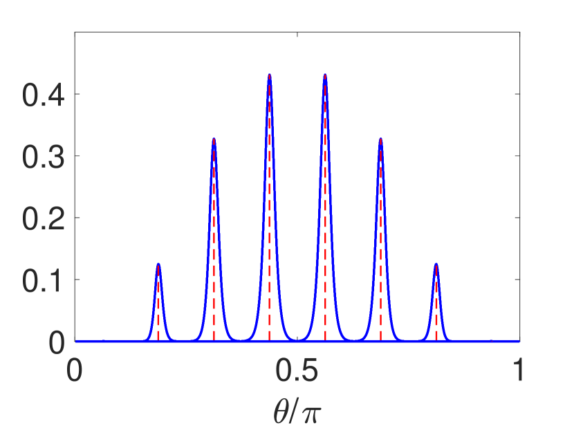
(a)

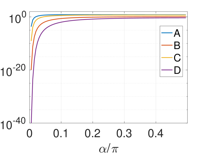
(b)

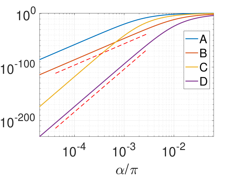
(c)

Figure 1: Illustration of results related to Theorem 2 for a sphere of radius $a=1$ with $p=1/2$. (a) Plot of $E_{fac}^{TZ}(\bm{x}(\alpha),\theta)$ versus $\theta/\pi$ for several values of $\alpha$ with $n_{\varphi}=20$ and $m=1.05$. Each curve peaks at $\theta=\alpha$, marked with a red vertical dashed line, and decays rapidly away from $\theta=\alpha$. (b) Plot of $E_{fac}^{TZ}(\bm{x}(\alpha),\alpha)$ versus $\alpha/\pi$ for (A): $n_{\varphi}=20$, $m=1.01$, (B): $n_{\varphi}=20$, $m=1.05$, (C): $n_{\varphi}=40$, $m=1.01$, (D): $n_{\varphi}=40$, $m=1.05$. (c) Same as (b) but with log scale over small values of $\alpha$. The two dashed red lines indicate the slopes $\alpha^{2n_{\varphi}}$ for $n_{\varphi}=20$ and $40$, respectively.

To the left in Fig. 1, we plot $E_{fac}^{TZ}(\bm{x}(\alpha),\theta)$ versus $\theta/\pi$ for several values of $\alpha$ for a sphere of radius $1$, with $p=1/2$. $E_{fac}^{TZ}(\bm{x}(\alpha),\theta)$ peaks at $\theta=\alpha$, and decays rapidly away from $\theta=\alpha$. The closer the evaluation point is to the surface (i.e. the closer $m$ is to $1$), the larger the maximum magnitude for a fixed number of discretization points $n_{\varphi}$. For a fixed $m$, the maximum magnitude decreases rapidly with $n_{\varphi}$. In the middle figure, we plot $E_{fac}^{TZ}(\bm{x}(\alpha),\alpha)$ versus $\alpha/\pi$ for the combinations of $n_{\varphi}=20$ and $40$ and $m=1.01$ and $1,05$. In the rightmost plot, we zoom in to see the behavior for small values of $\alpha$. As $\sin\alpha\approx\alpha$ for small $\alpha$, we expect to see a decay proportional to $\alpha^{2n_{\varphi}}$, and we indicate these slopes in the plot for the two values of $n_{\varphi}$.

From Corollary 2, we have the result that the trapezoidal rule error $E_{\bm{\gamma}}^{TZ}$ is bounded by a constant times $E_{fac}^{TZ}(\bm{x}(\alpha),\alpha)$, and in the plots we can see the fast decay of $E_{fac}^{TZ}(\bm{x}(\alpha),\alpha)$ with decreasing $\alpha$.

Let us now consider the Gauss-Legendre rule error. Write $E_{\bm{\gamma}}^{GL}$ Eq. 32 from Error estimate 3 as

$$E_{\bm{\gamma}}^{GL}(f,p,n_{t},\bm{x}) =\frac{4\pi}{\Gamma(p)}(2n_{t}+1)^{p-1}\int_{E_{2}}\mathinner{\!\left\lvert f\left(t_{0}(\varphi,\bm{x}),\varphi\right)\right\rvert}E_{fac}^{GL}(\bm{x},\varphi)\operatorname{d\!}\varphi,$$ (57)

where

$$E_{fac}^{GL}(\bm{x},\varphi)=\mathinner{\!\left\lvert G_{\bm{\gamma},1}\left(t_{0}(\varphi),\varphi,\bm{x}\right)\right\rvert}^{p}\frac{\mathinner{\!\left\lvert\sqrt{t_{0}(\varphi)^{2}-1}\right\rvert}^{1-p}}{\mathinner{\!\left\lvert t_{0}(\varphi)+\sqrt{t_{0}(\varphi)^{2}-1}\right\rvert}^{2n+1}}.$$ (58)

This term can be directly evaluated for points on the symmetry axis. For an evaluation point $\bm{x}=(0,0,z)$, we find that for a sphere of radius $a$,

$$E_{fac}^{GL}(\bm{x},\varphi)=\frac{1}{2a\mathinner{\!\left\lvert z\right\rvert}}\frac{1}{\mathinner{\!\left\lvert z^{2}-a^{2}\right\rvert}^{p-1}}\left(\frac{1}{\delta}\right)^{2n_{t}+1}$$ (59)

where $\delta=\mathinner{\!\left\lvert z\right\rvert}/a$ if $\mathinner{\!\left\lvert z\right\rvert}>a$ and $\delta=a/\mathinner{\!\left\lvert z\right\rvert}$ if $\mathinner{\!\left\lvert z\right\rvert}<a$. We use the result in Corollary 1 for this derivation. For details, see Appendix A. This result is independent of $\varphi$, and hence we have

$$E_{\bm{\gamma}}^{GL}(f,p,n_{t},\bm{x}) =\frac{4\pi}{\Gamma(p)}\frac{1}{2a\mathinner{\!\left\lvert z\right\rvert}}\frac{(2n_{t}+1)^{p-1}}{\mathinner{\!\left\lvert z^{2}-a^{2}\right\rvert}^{p-1}}\left(\frac{1}{\delta}\right)^{2n_{t}+1}\int_{E_{2}}\mathinner{\!\left\lvert f\left(t_{0}(\varphi,\bm{x}),\varphi\right)\right\rvert}\operatorname{d\!}\varphi.$$ (60)

This means that the Gauss-Legendre error $E^{GL}$ will strongly dominate over the trapezoidal rule error $E^{TZ}$ for evaluation points close to the symmetry axis, and the trapezoidal rule error can hence safely be ignored.

For a general axisymmetric surface, we cannot follow the same approach as for the sphere, were we could identify the two parametrization angles for the closest point on the surface, and furthermore show that $E_{fac}^{TZ}(\bm{x},\theta)$ attains its maximum value for that value of the polar angle $\theta$. As an evaluation point sufficiently close to a general axisymmetric surface approaches the $z$-axis, the closest point on the surface will however be the north or the south pole. Hence, it is interesting to investigate this limit.

Theorem 3.

Let $E_{fac}^{TZ}(\bm{x},\theta)$ be defined as in Theorem 1, and assume $z$ of the evaluation point $\bm{x}=(x,y,z)\in\mathbb{R}^{3}$ such that $(b(\theta)\cos(\theta)-z)^{2}=(\tilde{b}-z)^{2}>0$ for $\theta\in\{[0,\beta]\cup[\pi-\beta,\pi]\}$, for some $\beta>0$. Then for this range of $\theta$ it holds

$$E_{fac}^{TZ}(\bm{x})\leq\frac{C}{(\tilde{b}-z)^{2(p+n_{\varphi})}}(\rho a(\theta)\sin\theta)^{n_{\varphi}}.$$ (61)

In the limit as $\rho\rightarrow 0$ or $\tilde{a}=a(\bar{\theta})\sin(\bar{\theta})\rightarrow 0$, or both, we have $E_{fac}^{TZ}(\bm{x})\rightarrow 0$.

Proof: (Theorem 3) We start with Eq. 51 and rewrite $\lambda$ as $\lambda=(\tilde{a}/\rho+\rho/\tilde{a})/2+(\tilde{b}-z)^{2}/(2\tilde{a}\rho)$. As it is assumed $(\tilde{b}-z)^{2}>0$, we can use the simple estimate

$$\lambda\geq 1+\frac{(\tilde{b}-z)^{2}}{2\tilde{a}\rho}>\frac{(\tilde{b}-z)^{2}}{2\tilde{a}\rho},$$

and hence

$$E_{fac}^{TZ}(\bm{x},\theta)<\frac{C}{(\tilde{a}^{2}+\rho^{2}+(\tilde{b}-z)^{2})^{p}}\left(\frac{\tilde{a}\rho}{(\tilde{b}-z)^{2}}\right)^{n_{\varphi}}<\frac{C}{(\tilde{b}-z)^{2(p+n)}}\left(\tilde{a}\rho\right)^{n_{\varphi}},$$ (62)

which is the desired result.

For general axisymmetric surfaces, we have not been able to prove that the trapezoidal error vanishes as the evaluation point approaches the $z$-axis, as we have done for the sphere in Corollary 2. From the theorem above, we have the result that $E_{fac}^{TZ}(\bm{x},\theta)$ vanishes as $\bm{x}$ approaches the $z$-axis for some range of $\theta$, under some assumption on the $z$-coordinate. We have however not proven for which value of $\theta$ the maximum of $E_{fac}^{TZ}(\bm{x},\theta)$ is attained. We do conjecture that this $\theta\rightarrow\{0,\pi\}$ as the evaluation point approaches the $z$-axis for $z<0$ and $z>0$, respectively, as this $\theta$ is the parameter for the point on the surface closest to the evaluation point.

Numerically, we note that the trapezoidal error contribution to the total error estimate decays rapidly as the evaluation point approaches the $z$-axis also for general axisymmetric surfaces.

5.3 Simplified error estimate for a spherical surface

In this section, we will present a simplified error estimate for a spherical surface, and then discuss the derivation of it, starting from Error estimate 3.

Error estimate 4.

Let $\gamma(t,\varphi)=\bm{\gamma}^{\circ,A}(\theta(t),\varphi)$, where $\bm{\gamma}^{\circ,A}$ is the sphere parametrized as in Eq. 35 with $a(\theta)=b(\theta)=a$, and $\theta(t)=\pi-\cos^{-1}(t)$. Consider the integral in Eq. 6 with $k\equiv 1$ and $\sigma\equiv 1$ such that $f(t,\varphi)=\mathinner{\!\left\lVert\partial\bm{\gamma}/\partial t\times\partial\bm{\gamma}/\partial\varphi\right\rVert}=a^{2}$, with the evaluation point $\bm{x}=(x,y,z)\in\mathbb{R}^{3}$ not on $\gamma$.

Introduce $\zeta=\|\bm{x}\|=\sqrt{x^{2}+y^{2}+z^{2}}$ and an even integer $n$. The error in approximating the integral with the $n_{t}=n/2$ point Gauss-Legendre rule in the $t$-direction and the $n_{\varphi}=n$-point trapezoidal rule in the $\varphi$ direction can be estimated as

$$E_{sphere}(\zeta,a,p,n)=\frac{8\pi}{\Gamma(p)}n^{p-1}\frac{n!!}{(n+1)!!}\frac{a^{2}}{\mathinner{\!\left\lvert\zeta^{2}-a^{2}\right\rvert}^{p}}\left(\frac{1}{\delta}\right)^{n},$$ (63)

where $\delta=\zeta/a$ if $\zeta>a$ and $\delta=a/\zeta$ if $\zeta<a$.

Remark 7.

Note that this error estimate only depends on the evaluation point through $\zeta=\|\bm{x}\|$. This means that the error is estimated to decay equally in all directions as we move away from the sphere. This is only a good approximation under the map $t=-\cos(\theta)$, and not under the linear map, as will be discussed in section 7.1.

To derive the simplified estimate, we will use the assumption that the error only depends on the distance to the sphere, and will pick an evaluation point that yields the simplest expressions to work with. We will start by considering the trapezoidal rule error at a point $\bm{x}=(x,y,0)$; in this case $\zeta$ corresponds to the distance from the z-axis that was previously denoted by $\rho$, so we will continue with this notation, assuming $\rho^{2}=x^{2}+y^{2}\neq a$. The expression for $E_{fac}^{TZ}(\bm{x},\theta)$ is given in Eq. 50, but we will start with the equivalent expression in Eq. 53. For this case we obtain $\lambda=(\rho/a+a/\rho)/(2\sin\theta)=(\delta+1/\delta)/(2\sin\theta)$ where we let $\delta=\rho/a$ if $\rho>a$ and $\delta=a/\rho$ if $\rho<a$, such that $\delta>1$. With this, we have

$$\lambda^{2}-1=\left(\frac{1}{2\sin\theta}\left(\delta-\frac{1}{\delta}\right)\right)^{2}+\frac{\cos^{2}\theta}{\sin^{2}\theta}.$$ (64)

From Theorem 2, we know that $E_{fac}^{TZ}(\bm{x},\theta)$ will attain its maximum at $\theta=\pi/2$ for the chosen evaluation point. At this value of $\theta$, the last term vanishes. Ignoring that term we get $\lambda+\sqrt{\lambda^{2}-1}\approx\delta/\sin\theta$ with equality at $\theta=\pi/2$. If we use this approximation, and evaluate the part of $E_{fac}^{TZ}$ that is taken to the power of $p$ at $\theta=\pi/2$, we obtain

$$E_{fac}^{TZ}(\bm{x},\theta)\approx\frac{1}{\mathinner{\!\left\lvert\rho^{2}-a^{2}\right\rvert}^{p}}\left(\frac{\sin\theta}{\delta}\right)^{n}.$$

Now, under the map $t=-\cos(\theta)$ an approximation to the trapezoidal rule error will be

$$E_{\bm{\gamma}}^{TZ}(a^{2},p,n,\bm{x}) \approx\frac{4\pi}{\Gamma(p)}n^{p-1}\frac{1}{\mathinner{\!\left\lvert\rho^{2}-a^{2}\right\rvert}^{p}}\int_{-1}^{1}\left(\frac{\sin\theta(t)}{\delta}\right)^{n}\,dt$$ (65)

$$=\frac{4\pi}{\Gamma(p)}n^{p-1}\frac{1}{\mathinner{\!\left\lvert\rho^{2}-a^{2}\right\rvert}^{p}}\left(\frac{1}{\delta}\right)^{n}\int_{-1}^{1}\left(\sqrt{1-t^{2}}\right)^{n}\,dt.$$ (66)

Under the coordinate transformation $t=\sin\beta$, the integral can be written as

$$\int_{-\pi/2}^{\pi/2}(\cos\beta)^{n+1}\,d\beta.$$ (67)

Using that for $q>1$,

$$\int_{-\pi/2}^{\pi/2}(\cos\beta)^{q}\,d\beta=\frac{q-1}{q}\int_{-\pi/2}^{\pi/2}(\cos\beta)^{q-2}\,d\beta,$$

we obtain

$$\int_{-1}^{1}\left(1-t^{2}\right)^{n/2}\,dt=2\frac{n(n-2)\cdots 2}{(n+1)(n-1)\cdots 3}=\frac{2n!!}{(n+1)!}$$

and in total we get

$$E_{\bm{\gamma}}^{TZ}(a^{2},p,n,\bm{x})\approx\frac{8\pi}{\Gamma(p)}n^{p-1}\frac{n!!}{(n+1)!}\frac{a^{2}}{\mathinner{\!\left\lvert\rho^{2}-a^{2}\right\rvert}^{p}}\left(\frac{1}{\delta}\right)^{n}.$$ (68)

We will now continue by estimating the size of the Gauss-Legendre rule error. We write $E_{\bm{\gamma}}^{GL}$ from Error estimate 3 as in Eq. 57, with $E_{fac}^{GL}(\bm{x},\varphi)$ defined in Eq. 58.

Again, picking an evaluation point at the equator, we can derive the approximation

$$E_{\bm{\gamma}}^{GL}(a^{2},p,n,\bm{x})\approx\frac{8\pi}{\Gamma(p)}(n+1)^{p-1}\frac{n!!}{(n+1)!}\frac{a^{2}(\rho/a+a/\rho)}{\mathinner{\!\left\lvert\rho^{2}-a^{2}\right\rvert}^{p}}\left(\frac{1}{\delta}\right)^{n+1},$$ (69)

where $\rho=\|\bm{x}\|$. The details of this derivation is given in Appendix A.

Comparing Eq. 68 ($n=n_{\varphi}$) and Eq. 69 ($n=2n_{t}$), the expressions are very similar. The ratio is $E_{\bm{\gamma}}^{GL}/E_{\bm{\gamma}}^{TZ}=((n+1)/n)^{p-1}(1+1/\delta^{2})$.

This means that the contributions of the two errors are of about equal size for evaluation points in the $xy$-plane at $z=0$, as opposed to the case of evaluation points at the $z$-axis, where the contribution for the trapezoidal rule $E_{\bm{\gamma}}^{TZ}$ vanishes. The total error is however approximately equal for the same $\zeta=\|\bm{x}\|$. Since there is some overestimation of the errors, we have chosen to estimate the full error as a function of $\zeta$ by the derived expression for the trapezoidal rule error at the equator, as is given in (63) in Error estimate 4. The accuracy of this estimate will be numerically evaluated in Section 7.1.

6 Numerical evaluation of the error estimate

An estimate $E_{\bm{\gamma}}^{EST}$ for the quadrature error $E_{\bm{\gamma}}^{Q}$ in the evaluation of a layer potential was given in Error estimate 3. The integrals in (31)-(32) adding up to $E_{\bm{\gamma}}^{EST}$ can however not be evaluated analytically, and we need to introduce an approximation that is sufficiently precise and computationally cheap to evaluate. For general surfaces, we do not have access to analytical expressions for the roots appearing in the estimate. Hence, they must be computed using a numerical root finding procedure, and it will be of interest to minimize the number of root evaluations.

The integrand in (31) is not well defined for evaluation points along the symmetry axis for an axisymmetric surface, as was discussed in section 5.2. We proved that the contribution from the trapezoidal error (31) vanishes in the limit of the target point approaching the symmetry axis of a sphere (Corollary 2). For a general axisymmetric surface, we were able to prove only a weaker result but we quantified the contribution of the trapezoidal error (31) compared to the contribution of the Gauss-Legendre error (32) by numerical experiments. Also here we find that the first quantity decays very rapidly as the evaluation point approaches the z-axis, depending also on the distance of the evaluation point from the surface. To be more precise, the problematic target points lie in the region where $\rho\rightarrow 0$ or/and $a(\theta)\sin(\theta)\rightarrow 0$ (see Theorem 3) geometrically represented by the cones with apices at the poles and increasing width inside or outside the surface respectively for the interior or exterior problem. To see why, consider a number of target points placed in the normal direction starting from a grid point $\gamma(t^{*},\varphi^{*})$; it is clear that they will all refer to the same closest grid point, but $\rho$ (the distance from the z-axis) will increase together with the distance from the surface. In practical applications we will safely ignore the trapezoidal rule contribution for the evaluation points $\bm{x}$ such that

$$\frac{\rho}{A}<\frac{K_{c}\pi}{n_{t}}\min_{(t,\varphi)}\mathinner{\!\left\lVert\bm{\gamma}(t,\varphi)-\bm{x}\right\rVert},$$ (70)

where $K_{c}$ is a fixed constant, $\rho$ the distance to the $z$-axis and $A$ a representative radius/length scale. This procedure is not very sensitive to the choice of $A$ and $K_{c}$, as there is a rather wide range where the trapezoidal rule error contribution is negligible but it is still numerically stable to compute the error estimate. Practically, to evaluate the distance between the target point and the surface it is sufficient to approximate the minimum in (70) by the minimum over the surface grid points only.

When considering non-axisymmetric surfaces, the situation is much less predictable and we need a different strategy. This is based on using a local approximation of the surface centered away from the poles; in this way all the quantities needed for the estimate evaluation are locally well defined, and the singularities mentioned above are eluded. How to numerically compute such an approximation will be further discussed in the next subsections, where we describe how to practically evaluate the two error contributions (31) and (32), that add up to the total error. We start by the approximation of the integrals before we discuss the root finding.

6.1 Approximation of integrals in the error estimate

In this section, we discuss how to approximate the integrals in (31)-(32), to be able to efficiently compute a sufficiently precise estimate $E_{\bm{\gamma}}^{EST}$ for the quadrature error $E_{\bm{\gamma}}^{Q}$ as defined in Error estimate 3.

Given an evaluation point $\bm{x}\in\mathbb{R}^{3}$, we start by identifying $\bm{x}^{*}\in\mathbb{R}^{3}$, the closest discrete point on the surface $\bm{\gamma}$, and the parameters $t^{*}$, $\varphi^{*}$ such that $\bm{\gamma}(t^{*},\varphi^{*})=\bm{x}^{*}$. This means that $t^{*}$ will be one of the $n_{t}$ Gauss-Legendre quadrature nodes, and $\varphi^{*}$ will be one of the $n_{\varphi}$ (equidistant) trapezoidal rule quadrature nodes. Loosely speaking, the contribution to the quadrature error will have a peak around $\bm{x}^{*}$. What this means is that $\operatorname{est}^{TZ}(\varphi_{0}(t,\bm{x}),n_{\varphi},p)$ in the integral over $t$ in (31) will have a peak close to $t=t^{*}$, and decay rapidly away from $t^{*}$ due to the variation in $\varphi_{0}(t,\bm{x})$. Similarly $\operatorname{est}^{GL}(t_{0}(\varphi,\bm{x}),n_{t},p)$ will have a peak close to $\varphi=\varphi^{*}$, decaying rapidly away from $\varphi^{*}$ due to the variation in $t_{0}(\varphi,\bm{x})$. Let us here remind that the roots $t_{0}(\varphi,\bm{x})$ and $\varphi_{0}(t,\bm{x})$ are roots to $R^{2}(t,\varphi,\bm{x})$ with one variable kept fixed, as defined in Error estimate 3, and further denote

$$t_{0}^{*}=t_{0}(\varphi^{*},\bm{x}),\quad\varphi_{0}^{*}=\varphi_{0}(t^{*},\bm{x}).$$ (71)

We now assume that $\operatorname{est}^{TZ}$ is the most rapidly varying factor in the integrand in (31), and similarly for $\operatorname{est}^{GL}$ in (32), and approximate

$$E_{\bm{\gamma}}^{TZ}(f,p,n_{\varphi},\bm{x}) \approx\mathinner{\!\left\lvert f\left(t^{*},\varphi_{0}^{*}\right)G_{\bm{\gamma},2}\left(t^{*},\varphi_{0}^{*},\bm{x}\right)^{p}\right\rvert}\int_{E_{1}}\operatorname{est}^{TZ}(\varphi_{0}(t,\bm{x}),n_{\varphi},p)\operatorname{d\!}t,$$ (72)

$$E_{\bm{\gamma}}^{GL}(f,p,n_{t},\bm{x}) \approx\mathinner{\!\left\lvert f\left(t_{0}^{*},\varphi^{*}\right)G_{\bm{\gamma},1}\left(t_{0}^{*},\varphi^{*},\bm{x}\right)^{p}\right\rvert}\int_{E_{2}}\operatorname{est}^{GL}(t_{0}(\varphi,\bm{x}),n_{t},p)\operatorname{d\!}\varphi.$$ (73)

This is typically a good approximation, unless the surface grid is very stretched such that the grid resolutions on the surface in the two directions are very different, in which case the geometry factors can vary rapidly as well.

Now, we want to find a simple expression for how $t_{0}(\varphi,\bm{x})$ varies with $\varphi$ around $\varphi=\varphi^{*}$. If we replace $\bm{\gamma}$ with its bivariate linear approximation around $(t^{*},\varphi^{*})$ in the definition of the squared distance function (20), we get a quadratic equation that we can solve to find the root. From here, we find the approximation

$$t_{0}^{L}(\varphi)=t^{*}-\frac{b}{2c}\pm i\frac{\sqrt{4ac-b^{2}}}{2c},$$ (74)

where, with $\Delta\varphi=\varphi-\varphi^{*}$, and $\bm{r}=\bm{x}^{*}-\bm{x}=\bm{\gamma}(t^{*},\varphi^{*})-\bm{x}$,

$$a=a(\Delta\varphi) =\mathinner{\!\left\lVert\bm{r}\right\rVert}^{2}+2\left(\bm{r}\cdot\partial_{\varphi}\bm{\gamma}(t^{*},\varphi^{*})\right)\Delta\varphi+\mathinner{\!\left\lVert\partial_{\varphi}\bm{\gamma}(t^{*},\varphi^{*})\right\rVert}^{2}\Delta\varphi^{2},$$

$$b=b(\Delta\varphi) =2\left(\bm{r}\cdot\partial_{t}\bm{\gamma}(t^{*},\varphi^{*})\right)+2\left(\partial_{\varphi}\bm{\gamma}(t^{*},\varphi^{*})\cdot\partial_{t}\bm{\gamma}(t^{*},\varphi^{*})\right)\Delta\varphi,$$

$$c=c(\Delta\varphi) =\mathinner{\!\left\lVert\partial_{t}\bm{\gamma}(t^{*},\varphi^{*})\right\rVert}^{2}.$$

The root $t_{0}^{*}$ is by definition the root at $\varphi=\varphi^{*}$, and in practice, as will be discussed in the next subsection, at least an accurate approximation to it, while $t_{0}^{L}(\varphi^{*})$ is a simpler approximation. In order to better capture the magnitude of the peak of $\operatorname{est}^{GL}(t_{0}(\varphi,\bm{x}),n_{t},p)$, we want to use this more accurate value, but we also want to use the simple dependence on $\varphi$. This leads us to define

$$\tilde{t}_{0}(\varphi)=t_{0}^{*}-t_{0}^{L}(\varphi^{*})+t_{0}^{L}(\varphi).$$ (75)

See (AFKLINTEBERG20221, ) for more details and a discussion regarding the effect of making these approximations.

The same approximations can naturally be made to define $\tilde{\varphi}_{0}(t)$, an approximation to $\varphi_{0}(t,\bm{x})$. Away from $t=t^{*}$, we have $\mathinner{\!\left\lvert Im\,\tilde{\varphi}_{0}(t)\right\rvert}\sim k~{}\mathinner{\!\left\lvert t-t^{*}\right\rvert}$, where $k=\mathinner{\!\left\lVert\partial_{t}\bm{\gamma}(t^{*},\varphi^{*})\right\rVert}/\mathinner{\!\left\lVert\partial_{\varphi}\bm{\gamma}(t^{*},\varphi^{*})\right\rVert}$, and hence $\mathinner{\!\left\lvert Im\,\tilde{t}_{0}(\varphi)\right\rvert}\sim k^{-1}~{}\mathinner{\!\left\lvert\varphi-\varphi^{*}\right\rvert}$. This means that $\operatorname{est}^{TZ}(\tilde{\varphi}_{0}(t),n_{\varphi},p)$ decays as

$$e^{-n_{\varphi}\mathinner{\!\left\lvert Im\,\tilde{\varphi}_{0}(t)\right\rvert}}\sim e^{-n_{\varphi}k~{}\mathinner{\!\left\lvert t-t^{*}\right\rvert}}.$$ (76)

Given this decay, it is a reasonable approximation to expand the interval of integration in (72) from $[-1,1]$ to $[-\infty,\infty]$, as the tails will be negligible, and we approximate the integral in (72) by

$$\int_{0}^{\infty}\operatorname{est}^{TZ}\left(\tilde{\varphi}_{0}(t^{*}-s),n_{\varphi},p\right)\operatorname{d\!}s+\int_{0}^{\infty}\operatorname{est}^{TZ}\left(\tilde{\varphi}_{0}(t^{*}+s),n_{\varphi},p\right)\operatorname{d\!}s.$$ (77)

With the variable transformation $x=n_{\varphi}ks$, we can write

$$\int_{0}^{\infty}\operatorname{est}^{TZ}\left(\tilde{\varphi}_{0}(t^{*}\pm s)\right)\operatorname{d\!}s =\frac{1}{n_{\varphi}k}\int_{0}^{\infty}h^{TZ}_{\pm}(x)e^{-x}\operatorname{d\!}x,$$ (78)

where $h^{TZ}_{\pm}(x)=\operatorname{est}^{TZ}\left(\tilde{\varphi}_{0}(t^{*}\pm x/(n_{\varphi}k))\right)e^{x}$. Gauss-Laguerre quadrature is a Gaussian quadrature for integrals of this type (NIST:DLMF, , $\mbox{\rm\bf S}_{3}$.5(v)), and we find that is is sufficiently accurate to evaluate each of the integrals of $h^{TZ}_{+}(x)$ and $h^{TZ}_{-}(x)$ with 8 quadrature nodes.

For the Gauss-Legendre estimate, we have the bound AfKlinteberg2016quad

$$\operatorname{est}^{GL}(t_{0},n,p) =\frac{4\pi}{\Gamma(p)}\mathinner{\!\left\lvert\frac{2n+1}{\sqrt{t_{0}^{2}-1}}\right\rvert}^{p-1}\mathinner{\!\left\lvert t_{0}+\sqrt{t_{0}^{2}-1}\right\rvert}^{-(2n+1)}$$

$$\leq\frac{4\pi}{\Gamma(p)}(2n)^{p-1}e^{-2n\mathinner{\!\left\lvert\operatorname{Im}t_{0}\right\rvert}}.$$ (79)

Hence, with $t_{0}(\varphi,\bm{x})$ approximated with $\tilde{t}_{0}(\varphi)$, we have an estimated decay $e^{-2n_{t}k^{-1}~{}\mathinner{\!\left\lvert\varphi-\varphi^{*}\right\rvert}}$. Based on this decay we use the variable transformation $x=2n_{t}k^{-1}s$, and write the approximation of the integral in (73) as

$$\frac{k}{2n_{t}}\left[\int_{0}^{\infty}h^{GL}_{-}(x)e^{-x}\operatorname{d\!}x+\int_{0}^{\infty}h^{GL}_{+}(x)e^{-x}\operatorname{d\!}x\right],$$ (80)

where $h^{GL}_{\pm}(x)=\operatorname{est}^{GL}\left(\tilde{t}_{0}(\varphi^{*}\pm xk/(2n_{t})),n_{t},p\right)e^{x}$. Again, each of these integrals is approximated with an $8$-point Gauss-Laguerre quadrature rule.

In (AFKLINTEBERG20221, ), we used this strategy for the global trapezoidal rule discretization, and a different strategy for the panel based Gauss-Legendre quadrature. Here, we have a mix of the two quadrature rules, but both are used globally on the surface, and we have extended this approach to be used for both contributions to the error estimate. It remains now to discuss the root finding, and the evaluation of the factors in front of the integrals in (72)-(73).

6.2 Root finding

To evaluate the error estimate as described in the previous subsection, we need to determine $t_{0}^{*}=t_{0}(\varphi^{*},\bm{x})$ and $\varphi_{0}^{*}=\varphi_{0}(t^{*},\bm{x})$ as defined in (71). For spherical topologies, these roots are not always well defined, as introduced in 5.2 for axisymmetric geometries (where $\varphi_{0}(\theta,\bm{x})$ is not defined for evaluation points on the symmetry axis) and further discussed at the beginning of section 6 for general surfaces. For axisymmetric geometries we identified the problematic region in the cone defined by eq. (70): for these evaluation points we can ignore the trapezoidal error contribution and then we do not need to compute the roots $\varphi_{0}(\theta,\bm{x})$. We will then not consider these points in the following discussion. For a general surface, it is not so easy the determine a similar set, and we will proceed with a discrete approach as later discussed.

We will consider the $(\theta,\varphi)$ coordinate system, as also used in (7) in the definition of a generic surface $\gamma^{\circ}(\theta,\varphi)$. In (8), we define $\gamma(t,\varphi)=\gamma^{\circ}(\theta(t),\varphi)$. Hence, once a root $\theta_{0}$ has been determined, $t_{0}$ can be found using the inverse map from $\theta$ to $t$.

In Section 5, we derived analytical expressions for the roots of the squared distance function for special geometries: we have analytical expressions for $\theta_{0}$ only for a spherical surface, and for $\varphi_{0}$ for any axisymmetric surface. Hence, in general we need a numerical procedure to determine the roots, and we will define this procedure in the $(\theta,\varphi)$ coordinate system. Given an evaluation point $\bm{x}=(x,y,z)$, we define

$$R^{2}(\theta,\varphi,\bm{x})=(\gamma^{0}_{1}(\theta,\varphi)-x)^{2}+(\gamma^{0}_{2}(\theta,\varphi)-y)^{2}+(\gamma^{0}_{3}(\theta,\varphi)-z)^{2}.$$ (81)

Given a parametrization $\bm{\gamma}^{\circ}(\theta,\varphi)$, it is easy to solve $R^{2}(\theta,\varphi,\bm{x})=0$ using a one dimensional Newton’s method to find a root $\varphi_{0}$ given $\theta$, or similarly, to find a root $\theta_{0}$ given $\varphi$. Specifically, in our setting, we need to determine $\theta_{0}^{*}=\theta_{0}(\varphi^{*},\bm{x})$ and $\varphi_{0}^{*}=\varphi_{0}(\theta^{*},\bm{x})$, where $\theta^{*}=\theta(t^{*})$. We typically use an initial guess of $\theta^{*}+i/10$ for $\theta_{0}^{*}$, and correspondingly for $\varphi_{0}^{*}$. The iterations then usually converge with a strict tolerance in less than five iterations. However in rare cases, usually for evaluation points far away from the surface, it may happen that the iterations fail to converge, but most of the times it is sufficient to increase the magnitude of the imaginary part of the initial guess for the iterations to converge well.

If no parametrization is available and we know only the quadrature node values of $\bm{\gamma}^{\circ}$ at the $n_{t}\times n_{\varphi}$ nodes, we need to define an approximation $\bm{\tilde{}}\gamma^{\circ}(\theta,\varphi)$ that can be evaluated at different arguments of $\theta$ and $\varphi$, and that allows for differentiation to formulate Newton’s method. One way is to compute the spherical harmonics coefficients using a discrete transform Mohlenkamp99 . Evaluating the spherical harmonics expansion is however a global procedure with $O(n_{t}\,n_{\varphi})$ cost for arbitrary arguments, and this would need to be done at each step in the Newton iteration.

We can however use a local approach. In the Newton iteration, one of the variables, $\theta$ or $\varphi$ will be fixed. Assume that $\varphi=\varphi^{*}$ and introduce a $q$th order Taylor expansion in $\theta$, around $\theta=\theta^{*}$,

$$\bm{\tilde{\gamma}^{\circ}}(\theta,\varphi^{*})=\sum_{j=0}^{q}\frac{\left(\theta-\theta^{*}\right)^{j}}{j!}\mathinner{\dfrac{\partial{{}^{j}}\bm{\gamma^{\circ}}}{\partial{\theta^{j}}}}(\theta^{*},\varphi^{*}).$$ (82)

This approximation can be used in Newton’s method to determine an approximation to the root $\theta_{0}^{*}=\theta_{0}(\varphi^{*},\bm{x})$. Similarly, a Taylor expansion in $\varphi$ can be introduced to obtain an approximation to $\varphi_{0}^{*}=\varphi_{0}(\theta^{*},\bm{x})$. This is a solid strategy that eludes the pole singularities for any kind of geometry. Indeed, since the discretization is based on Gauss-Legendre nodes in the polar angle, the closest grid point where the expansion (82) is centered, will never be a pole, avoiding the above mentioned problems.

For this reason, we will use this approach for non-axisymmetric surfaces, even if we have a parametrization of $\bm{\gamma}^{\circ}$ available. In this case, the analytical expression for $\bm{\gamma}^{\circ}$ can however be used to determine the $q$ first partial derivatives of $\bm{\gamma}^{\circ}$. When this is not the case, the derivatives both with respect to $\theta$ and $\phi$, can be evaluated e.g from a spherical harmonics expansion. The advantage compared to using a global expansion is that we can evaluate these derivatives at all grid points in one sweep Sorgentone2018167 ; Schaeffer , and then use different local expansions when estimating the quadrature error for different evaluation points.

Once the roots have been determined, these Taylor expansions can also be used to evaluate the geometry factors in (72)-(73) as defined in (26)-(27). The roots $t_{0}^{*}$ and $\varphi_{0}^{*}$ are also needed to evaluate $f$ in (72)-(73). We recall that $f$ depends on the density $\sigma$, which may not be known analytically but be available at the grid points only (e.g. if $\sigma$ is a solution to a discretized integral equation). In this case, again, $f$ can either be approximated locally by a Taylor expansion, or globally by a spherical harmonics expansion.

7 Numerical experiments

In this section, we will compare the quadrature error estimate $E_{\bm{\gamma}}^{EST}$ defined in (30), and evaluated as discussed in the previous section, to the measured error $E_{\bm{\gamma}}^{Q}$ as defined in (29) for some different examples. The measured error $E_{\bm{\gamma}}^{Q}$ will be computed by using a reference solution on an upsampled grid with upsampling rate set to five.

As outlined in Remark 1, we will see that the estimate provides a good approximation of the error also for moderate values of $n_{t}$ and $n_{\varphi}$ as long as the geometry and the layer density are well resolved. We choose $n_{t}$ and $n_{\varphi}$ so that this is true for all the following numerical examples. For the rootfinding procedure, we follow the strategy presented in the previous section: the analytical expression for $\bm{\gamma}\circ$ is used when dealing with axisymmetric surfaces (excluding the trapezoidal error contribution for target points defined in (70)), and $\bm{\gamma}^{\circ}$ is locally approximated with a Taylor expansion for other geometries. In the first case, the parameters defining the cone in (70) will be kept fixed to $A=1$ and $K_{C}=10$. In the latter case, the order of the Taylor expansion will be fixed as $q=4$ (see eq. (82)), which is accurate enough for our purposes; an analysis of how the choice of $q$ can affect the accuracy of the roots can be found in (AFKLINTEBERG20221, ). In all the presented numerical tests we will use the analytical expression for the density.

7.1 A sphere

In the first example we consider the harmonic single layer potential

$$u(\bm{x})=\int_{S}\frac{\sigma(\bm{y})}{\mathinner{\!\left\lVert\bm{y}-\bm{x}\right\rVert}}\operatorname{d\!}S(\bm{y}),$$ (83)

evaluated near a sphere of radius $a=1$ with unit density, $\sigma(\bf{x})=1$. We want to compare the estimated error $E_{\bm{\gamma}}^{EST}$ to the actual measured error $E_{\bm{\gamma}}^{Q}$, using the full error estimate in (30), approximated as described in the previous section, and, for the cosine map, also the simplified error estimate (4), derived in Section 5.3. For this case, referring to eq. (30), $p=1/2$ and $f$ simplifies to

$$f(t,\varphi)=\mathinner{\!\left\lVert\mathinner{\dfrac{\partial{}\bm{\gamma}}{\partial{t}}}\times\mathinner{\dfrac{\partial{}\bm{\gamma}}{\partial{\varphi}}}\right\rVert}=\begin{cases}\frac{\pi}{2}\sin((t+1)\frac{\pi}{2}),\text{ if using the linear mapping \eqref{eq:linear_map}}\\ 1,\text{ if using the cosine mapping \eqref{eq:cos_map}.}\end{cases}$$

Fig. 2 shows the resulting surface grids and the different behavior of the quadrature error exterior to the sphere with discretizations using the linear and non-linear mapping $\theta(t)$ as given in (9)-(10), with $n_{t}=30$ and $n_{\varphi}=60$ points.

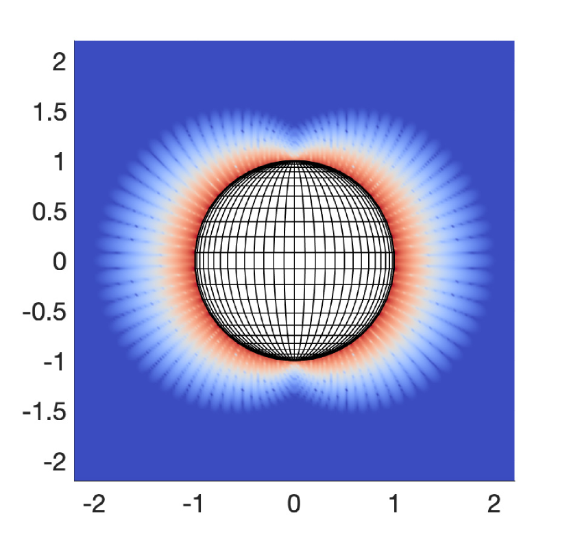
(a)

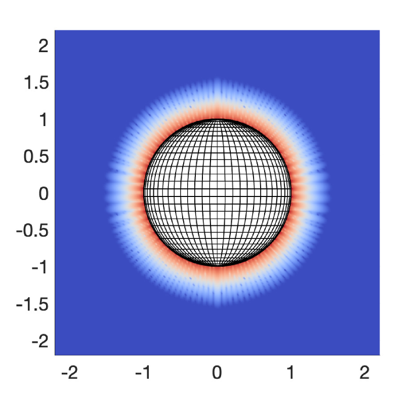
(b)

Figure 2: Error $E_{\bm{\gamma}}^{Q}$ ($\log 10$ scale) in computing the harmonic single layer potential with unit density on a plane at $y=0$ cutting a sphere of radius 1 discretized by using (a) the linear mapping, (b) the cosine mapping. In both cases, $n_{t}=30$ and $n_{\varphi}=60$.

The linear map clusters the grid points more towards the poles, and at a fixed distance from the sphere, the error is smaller in these regions, while the cosine mapping yields a more even error. In both cases we see oscillations in the error on a length scale of the grid size.

In Fig. 3, the full error estimate $E_{\bm{\gamma}}^{EST}$ from Error estimate 3, approximated as described in the previous section, is compared to the measured errors $E_{\bm{\gamma}}^{Q}$. The measured errors ($\log 10$ scale) are shown in one selected plane as colored fields, with the contours of the estimates drawn in black.

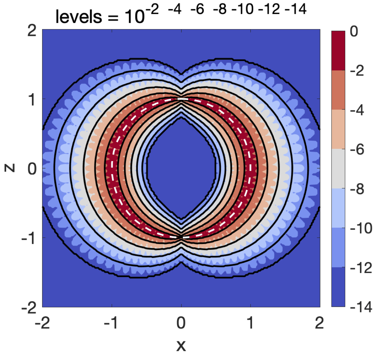
(a)

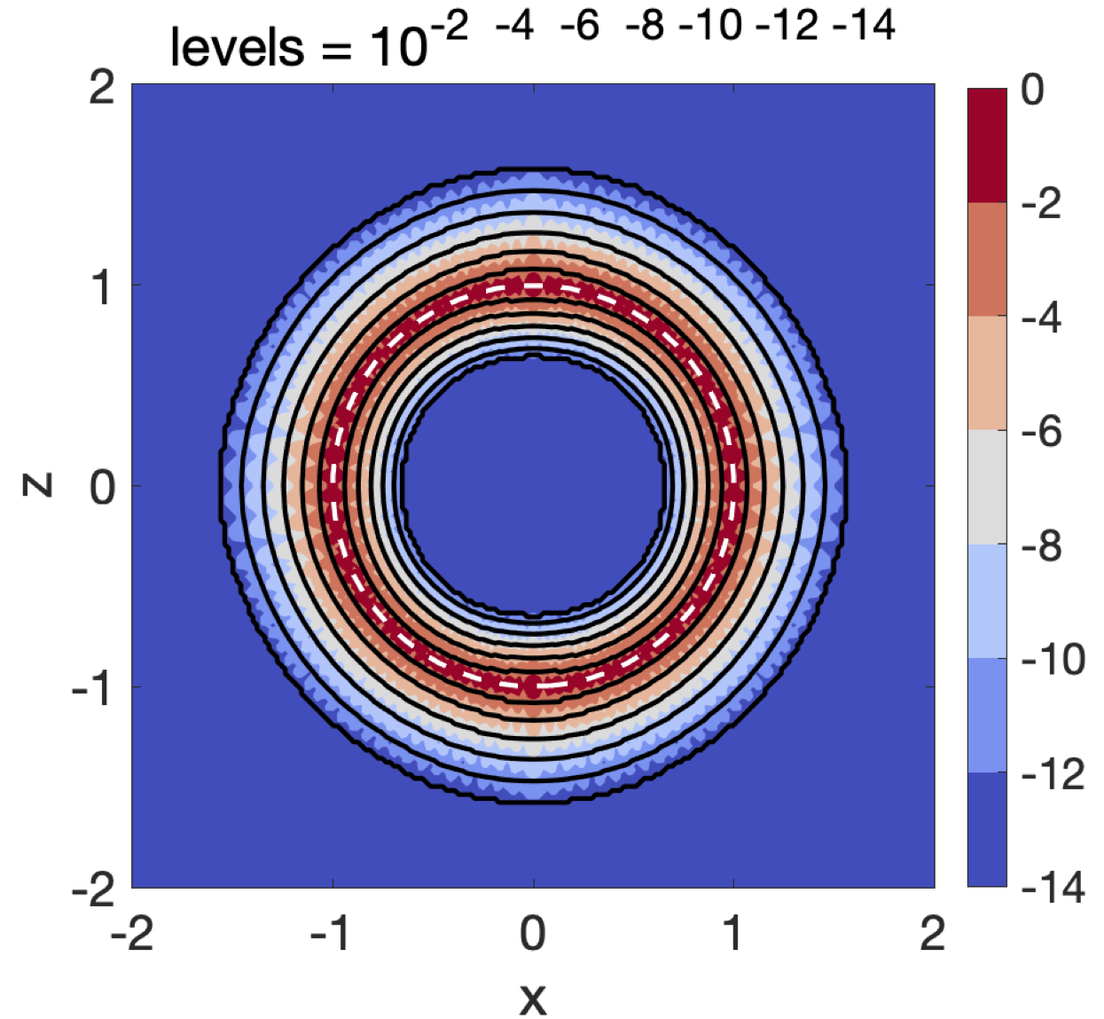
(b)

Figure 3: Error $E_{\bm{\gamma}}^{Q}$ (colors) and estimates $E_{\bm{\gamma}}^{EST}$ (black lines) plotted in $\log 10$ scale when computing the harmonic single layer potential with unit density over a sphere of radius 1 discretized by using (a) the linear mapping, (b) the cosine mapping. The results are shown for evaluation points in the $xz$-plane for $y=0$, both inside and outside of the sphere that is indicated with a dashed white line.

This is done for evaluation points both interior and exterior to the sphere, and the error estimates can be seen to work well. The contours of the estimate are smoothly enclosing the oscillatory error, with an over-estimation that is larger further out exterior to the sphere. Note however that the last contour is at an error level of $10^{-14}$, which is a very low level.

In Error estimate 4, we derived a simplified error estimate applicable to this case (when using the cosine map) that depends only on the radius $a$, the distance from the surface, the number of discretization points and the half-integer $p$, where $p=1/2$ for the integral in (83). In Fig. 4, we compare the error measured in a set of evaluation points to the simplified error estimate, both versus the distance to the surface (here a negative distance $d$ is used for interior point) for a fixed grid resolution, and versus the grid resolution for points at a fixed distance to the sphere.

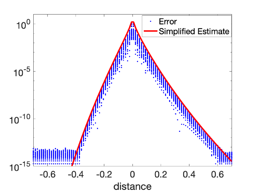
(a)

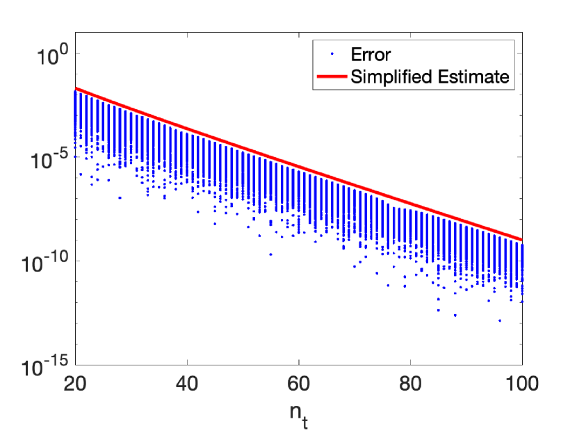
(b)

Figure 4: Measured quadrature errors $E_{\bm{\gamma}}^{Q}$ in evaluating (83) (using the cosine map) at a set of discrete evaluation points $\bm{x}\in\mathbb{R}^{3}$ (blue dots) and the simplified estimate (red lines); (a) varying distance to the sphere (negative values for interior) and fixed $n_{t}=30$ and (b) varying $n_{t}$ at the fixed distance $d=0.1$. Note that $n=n_{\varphi}=2n_{t}$ in the simplified estimate.

The discrete points are set using the parametrization for a sphere with radius $(1+d)$, over the full range of the polar angle $0\leq\theta\leq\pi$, but only over an angle sector in the azimuthal angle, $0\leq\varphi\leq\pi/n_{\varphi}$. The actual errors do not depend on $\varphi$, more than that there is an oscillation determined by the grid size, and this range is sufficient to cover the range of errors. Under the cosine-map, the error is much less dependent on $\theta$ compared to the linear mapping, but there is a variation, and we include the full range here. From the discrete dots, each representing a different evaluation point, we can see the range of errors for evaluation points at the same distance to the sphere. The simplified error estimate works better than we could expect, and gives a rather tight upper bound of the error.

7.2 A prolate spheroid

In the second example we consider an axisymmetric ellipsoid, a prolate spheroid, with ratio 3-1 between the long and short semi axes. Here the density function is given by

$$\sigma(\theta,\varphi)=1+\sin(6\varphi+\theta)\sin^{2}(\theta).$$ (84)

and is in Fig. 5(a) visualized on the surface by the black and white colormap. We can see how the varying density breaks the geometric symmetry of the problem. We first consider the quadrature error for evaluation points on a vertical wall placed at $y=1.02$, Fig. 5(a)-6(a), and then we place random evaluation points around the spheroid (Fig. 5(b)), and plot the error vs the estimate in Fig. 6(b). The latter is a simple way to indicate if the estimate over or under estimate the actual error. The red line indicates where error and estimate are equal, while the black lines indicate where they differ by factors 10 and 1/10, respectively.

In Fig. 5(a)-6(a) we are evaluating the harmonic single layer potential, eq. (83). In this case $p=1/2$ and $f(t,\varphi)=\sigma(t,\varphi)\mathinner{\!\left\lVert\mathinner{\dfrac{\partial{}\bm{\gamma}}{\partial{t}}}\times\mathinner{\dfrac{\partial{}\bm{\gamma}}{\partial{\varphi}}}\right\rVert}$, where $\sigma(t,\varphi)$ is obtained by mapping eq. (84) with the cosine map. In Fig. 5(b)-6(b) we consider the harmonic double layer potential

$$u(\bm{x})=\int_{S}\frac{{\bm{n}_{y}}\cdot(\bm{y}-\bm{x})\sigma(\bm{y})}{\mathinner{\!\left\lVert\bm{y}-\bm{x}\right\rVert}^{3}}\operatorname{d\!}S(\bm{y}),$$ (85)

for which $p=3/2$ and $f(t,\varphi)={\bm{n}_{\gamma}(t,\varphi)}\cdot(\bm{\gamma}(t,\varphi)-\bm{x})\sigma(t,\varphi)\mathinner{\!\left\lVert\mathinner{\dfrac{\partial{}\bm{\gamma}}{\partial{t}}}\times\mathinner{\dfrac{\partial{}\bm{\gamma}}{\partial{\varphi}}}\right\rVert}$.
In the first case $n_{t}=40$, in the second case $n_{t}=60$, and for both we set $n_{\varphi}=2n_{t}$. In both cases the estimates can predict very well the actual error. Moreover, it is clear that the density has an effect on the error, but still the simplification made in (72)-(73) is good enough to capture the behavior of the overall error.

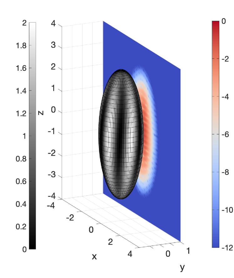
(a)

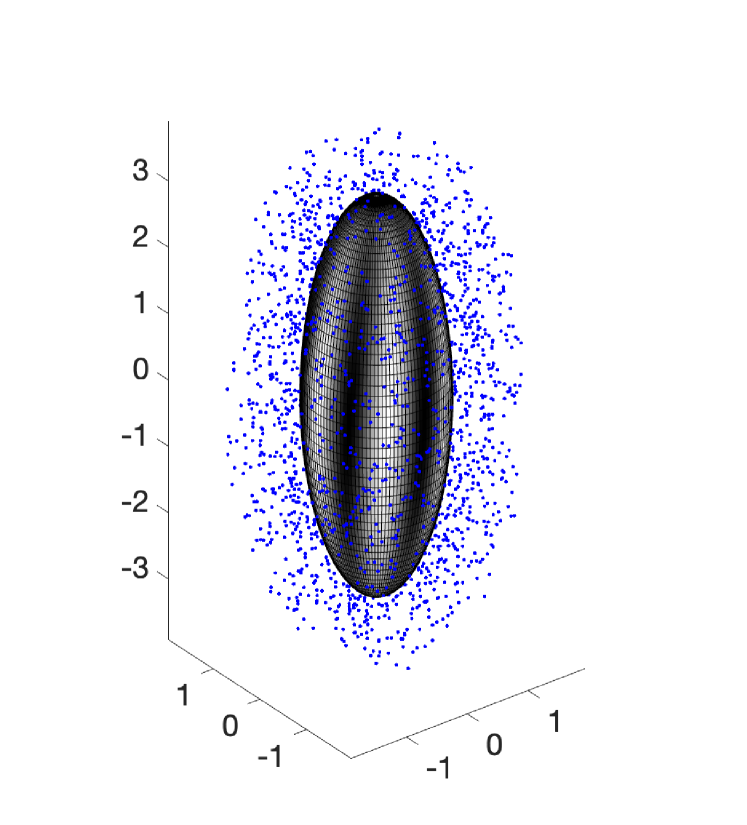
(b)

Figure 5: Target points considered when computing the harmonic single (a) and the double (b) layer potentials evaluated near a prolate spheroid. The black and white colormap represents the density given by eq. (84). The red and blue colormap represents the actual error evaluated on the target wall.

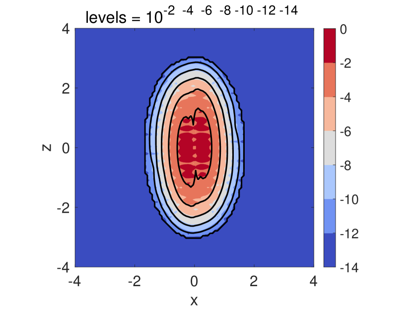
(a)

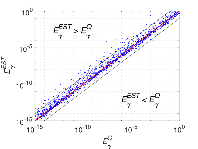
(b)

Figure 6: (a) Error $E_{\bm{\gamma}}^{Q}$ (colors) and estimates $E_{\bm{\gamma}}^{EST}$ (black lines) plotted in $\log 10$ scale when computing the harmonic single layer potential near the ellipsoid on a plane at $y=1.02$, shown in Fig. 5(a). (b) Estimates vs error in computing the harmonic double layer potential at random evaluation points showed in Fig. 5(b). The three lines from top to bottom indicate where the estimate of $E_{\bm{\gamma}}^{EST}$ is a factor of $10$, $1$ and $1/10$ times the measured value of $E_{\bm{\gamma}}^{Q}$. If the estimate was never underestimating the error, no dot would fall below the red line.

7.3 Non-axisymmetric geometry

In the last example we consider a non-axisymmetric geometry given by

$$\bm{\gamma}^{\circ}(\theta,\varphi)=\begin{cases}\rho(\theta,\varphi)\cos(\varphi)\sin(\theta)\\ \rho(\theta,\varphi)\sin(\varphi)\sin(\theta)\\ \rho(\theta,\varphi)\cos(\theta)\end{cases}$$ (86)

with $\rho(\theta,\varphi)=0.8+0.2e^{-3\text{Re}(Y_{3}^{2}(\theta,\varphi))}$ and $Y_{3}^{2}(\theta,\varphi)={1\over 4}{\sqrt{105\over 2\pi}}e^{2i\varphi}\sin^{2}(\theta)\cos(\theta)$. The surface is enclosed in a spherical shell of radius $a=1.46$, as shown in Fig. 7. Here we consider the modified Helmholtz equation $(\Delta-\omega^{2})u=0$, and compute the corresponding single layer potential:

$$u(\bm{x})=\int_{S}\frac{e^{-\omega\mathinner{\!\left\lVert\bm{y}-\bm{x}\right\rVert}}\sigma(\bm{y})}{\mathinner{\!\left\lVert\bm{y}-\bm{x}\right\rVert}}\operatorname{d\!}S(\bm{y}).$$ (87)

We use the cosine mapping and define $\bm{\gamma}(t,\varphi)=\bm{\gamma}^{\circ}(\cos^{-1}(-t),\varphi)$. For this case, referring to eq. (30), $p=1/2$ and $f(t,\varphi)=e^{-\omega\mathinner{\!\left\lVert\bm{\gamma}(t,\varphi)-\bm{x}\right\rVert}}\sigma(t,\varphi)\mathinner{\!\left\lVert\mathinner{\dfrac{\partial{}\bm{\gamma}}{\partial{t}}}\times\mathinner{\dfrac{\partial{}\bm{\gamma}}{\partial{\varphi}}}\right\rVert}$.

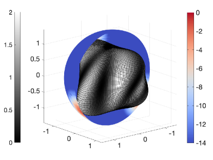
Figure 7: Half of the spherical shell enclosing the non axisymmetric shape defined in (86). The black and white colormap represents the density given by eq. (84).

We consider the case $\omega=3$ and the density function $\sigma$ given by eq. (84). In Fig. 8(a) we show the error and the estimates computed on the whole spherical shell, plotted here with the horizontal axis being the the azimuthal angle and the vertical axis being the polar angle. In Fig. 8(b) we zoom in on the white rectangle highlighted in Fig. 8(a), to better show the agreement between estimate and error.

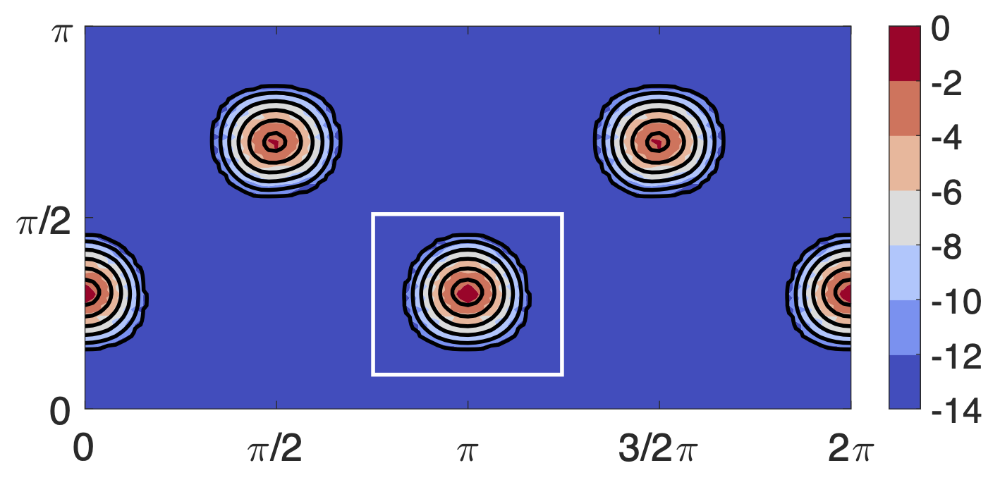
(a)

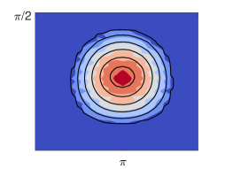
(b)

Figure 8: Error $E_{\bm{\gamma}}^{Q}$ (colors) and estimate $E_{\bm{\gamma}}^{EST}$ (black lines) in computing the modified Helmholtz potential with $\omega=3$ on the shell enclosing the non axisymmetric geometry eq. (86). The levels for the estimates contours are $10^{-2},10^{-4},10^{-6},10^{-8},10^{-10},10^{-12},10^{-14}$. In (b) we zoom in on the white rectangle drawn in (a).

8 Conclusions

In this paper, we studied the error incurred by numerically approximating layer potentials over surfaces of spherical topology. We have derived error estimates for discretizations with the trapezoidal rule in the azimuthal angle, and a Gauss-Legendre rule in a variable that maps to the polar angle. The framework for the derivation of the error estimates, and the practical evaluation there of, were introduced in AFKLINTEBERG20221 for surfaces of genus 1, discretized by either a global trapezoidal rule in both directions, or a panel based Gauss-Legendre rule. Here we extended this approach with special attention to the global parametrization. There is one component of the error estimate that cannot be directly evaluated for evaluation points on the symmetry axis of an axisymmetric surface. Starting by deriving analytical expressions for the roots of a squared distance function for a sphere, we were able to prove that this contribution vanishes at these points. We could also derive a simplified error estimate for the sphere, that shows the decay in error with the distance of the evaluation point to the sphere with a simple formula. Some analytical results were also extended to the more general case of an axisymmetric surface, and we devised a strategy for evaluating the error estimate for general surfaces, avoiding the difficulties associated with the discretization around the poles.

The error estimate does not have any unknown coefficients, but for each evaluation point for a general surface, two complex roots to the squared distance function must be computed using one-dimensional root finding. In numerical experiments, we have shown that the error estimate indeed estimates the actual error quite well, also for moderate numbers of discretization points. This is true for different layer potentials, various surfaces, and with a variable layer density. The simplified error estimate for the sphere is shown to give a tight upper bound for the error at a given distance from the spherical surface.

Appendix A Derivations for the Gauss-Legendre error

We consider a sphere of radius $a$ and the associated Gauss-Legendre error as defined in Eq. 57 with $E_{fac}^{GL}(\bm{x},\varphi)$ defined in Eq. 58. Under the map $t=-\cos\theta$, the squared distance function evaluates as

$$R^{2}(t,\varphi,\bm{x})=a^{2}-2a(\sqrt{1-t^{2}}(x\cos\varphi+y\sin\varphi)+tz)+x^{2}+y^{2}+z^{2}.$$

and $G_{\bm{\gamma},1}\left(t,\varphi,\bm{x}\right)=(\partial R^{2}/\partial t)^{-1}$. The root $\theta_{0}(\varphi,\bm{x})$ is given in Eq. 44, and $t_{0}(\varphi,\bm{x})=-\cos(\theta_{0}(\varphi,\bm{x}))$.

We start by considering an evaluation point at the symmetry axis, i.e. $\bm{x}=(0,0,z)$, $z\neq a$. For this case we get $\theta_{0}=\pm i\ln(\mathinner{\!\left\lvert z\right\rvert}/a)$ as given in Corollary 1. We get $t_{0}=(\delta+1/\delta)/2$, where we let $\delta=a/\mathinner{\!\left\lvert z\right\rvert}$ if $\mathinner{\!\left\lvert z\right\rvert}>a$, and $\delta=\mathinner{\!\left\lvert z\right\rvert}/a$ if $\mathinner{\!\left\lvert z\right\rvert}<a$, such that $\delta>1$. Hence, $\mathinner{\!\left\lvert\sqrt{t_{0}^{2}-1}\right\rvert}=(\delta-1/\delta)/2$, and $\mathinner{\!\left\lvert t_{0}+\sqrt{t_{0}^{2}-1}\right\rvert}=\delta$. Finally, we have $G_{\bm{\gamma},1}\left(t,\varphi,\bm{x}\right)=1/(2a\mathinner{\!\left\lvert z\right\rvert})$, and combined this yields the expression for $E_{fac}^{GL}(\bm{x},\varphi)$ given in Eq. 59.

Now, we instead consider an evaluation point at the equator, $\bm{x}=(0,y,0)$. We could however equally well pick $\bm{x}=(x,0,0)$, or $\bm{x}=(x,y,0)$ and would obtain the same final result with $\|\bm{x}\|=\rho$. With $\bm{x}=(0,y,0)$ we get

$$E_{fac}^{GL}(\bm{x},\varphi)=\frac{1}{(2a\mathinner{\!\left\lvert y\right\rvert}\mathinner{\!\left\lvert\sin\varphi\right\rvert})^{p}}\frac{\mathinner{\!\left\lvert\sqrt{t_{0}(\varphi)^{2}-1}\right\rvert}}{\mathinner{\!\left\lvert t_{0}(\varphi)\right\rvert}^{p}}\mathinner{\!\left\lvert\frac{1}{t_{0}(\varphi)+\sqrt{t_{0}(\varphi)^{2}-1}}\right\rvert}^{2n+1}.$$ (88)

The root $t_{0}(\varphi)=-\cos(\theta_{0}(\varphi))$ where $\theta_{0}(\varphi)$ is defined in Lemma 3, in Eq. 43. With $\bm{x}=(0,y,0)$, $\lambda$ in that expression simplifies to $\lambda=(\mathinner{\!\left\lvert y\right\rvert}/a+a/\mathinner{\!\left\lvert y\right\rvert})/(2\mathinner{\!\left\lvert\sin\varphi\right\rvert}=(\delta+1/\delta)/(2\mathinner{\!\left\lvert\sin\varphi\right\rvert})$ where we let $\delta=\mathinner{\!\left\lvert y\right\rvert}/a$ if $\mathinner{\!\left\lvert y\right\rvert}>a$ and $\delta=a/\mathinner{\!\left\lvert y\right\rvert}$ if $\mathinner{\!\left\lvert y\right\rvert}<a$, such that $\delta>1$. The expression for $\lambda^{2}-1$ then becomes the same as in Eq. 64, but with $\varphi$ instead of $\theta$. The peak of the error is at the closest point to $\bm{x}=(0,y,0)$, i.e. at $\varphi=\pi/2$, and also here, we ignore the last term in the expression for $\lambda^{2}-1$. With this we get that $\lambda+\sqrt{\lambda^{2}-1}\approx\delta/\mathinner{\!\left\lvert\sin\varphi\right\rvert}$. Introducing $\tilde{\delta}=\delta/\mathinner{\!\left\lvert\sin\varphi\right\rvert}$, and noting that the square roots are evaluated at points away from the branch cut, we have

$$t_{0}=i(\tilde{\delta}-1/\tilde{\delta})/2\qquad\sqrt{t_{0}^{2}-1}=i(\tilde{\delta}+1/\tilde{\delta})/2\qquad t_{0}+\sqrt{t_{0}^{2}-1}=i\tilde{\delta}.$$

Similarly to the derivation based on the trapezoidal error, we evaluate all terms in Eq. 88 except the last term at $\varphi=\pi/2$. We then have

$$E_{fac}^{GL}(\bm{x},\varphi)\approx\frac{1}{2}\frac{1}{(a\mathinner{\!\left\lvert y\right\rvert})^{p}}\frac{\mathinner{\!\left\lvert\delta+1/\delta\right\rvert}}{\mathinner{\!\left\lvert\delta-1/\delta\right\rvert}^{p}}\frac{\mathinner{\!\left\lvert\sin\varphi\right\rvert}^{2n+1}}{\delta^{2n+1}}.$$ (89)

Inserting into Eq. 57 and using

$$\int_{0}^{2\pi}\mathinner{\!\left\lvert\sin\varphi\right\rvert}^{2n_{t}+1}\operatorname{d\!}\varphi=\int_{0}^{2\pi}\mathinner{\!\left\lvert\cos\varphi\right\rvert}^{2n_{t}+1}\operatorname{d\!}\varphi=2\int_{-\pi/2}^{\pi/2}(\cos\varphi)^{2n_{t}+1}\operatorname{d\!}\varphi$$

we can identify the integral in Eq. 67. With $f=a^{2}$ the total result becomes $E^{GL}(\bm{\gamma},a^{2},p,2n_{t},\bm{x})$ as given in Eq. 69.

References

- \bibcommenthead
- (1) af Klinteberg, L., Sorgentone, C., Tornberg, A.-K.: Quadrature error estimates for layer potentials evaluated near curved surfaces in three dimensions. Computers & Mathematics with Applications 111, 1–19 (2022). https://doi.org/10.1016/j.camwa.2022.02.001
- (2) af Klinteberg, L., Tornberg, A.-K.: A fast integral equation method for solid particles in viscous flow using quadrature by expansion. Journal of Computational Physics 326, 420–445 (2016). https://doi.org/10.1016/j.jcp.2016.09.006
- (3) Corona, E., Greengard, L., Rachh, M., Veerapaneni, S.: An integral equation formulation for rigid bodies in Stokes flow in three dimensions. Journal of Computational Physics 332, 504–519 (2017). https://doi.org/10.1016/j.jcp.2016.12.018
- (4) Sorgentone, C., Tornberg, A.-K.: A highly accurate boundary integral equation method for surfactant-laden drops in 3D. Journal of Computational Physics 360, 167–191 (2018). https://doi.org/10.1016/j.jcp.2018.01.033
- (5) Sorgentone, C., Vlahovska, P.M.: Tandem droplet locomotion in a uniform electric field. Journal of Fluid Mechanics 951 (2022). https://doi.org/10.1017/jfm.2022.875
- (6) Rahimian, A., Veerapaneni, S.K., Zorin, D., Biros, G.: Boundary integral method for the flow of vesicles with viscosity contrast in three dimensions. Journal of Computational Physics 298, 766–786 (2015). https://doi.org/10.1016/j.jcp.2015.06.017
- (7) Veerapaneni, S.: Integral equation methods for vesicle electrohydrodynamics in three dimensions. Journal of Computational Physics 326, 278–289 (2016). https://doi.org/10.1016/j.jcp.2016.08.052
- (8) Donaldson, J.D., Elliott, D.: A unified approach to quadrature rules with asymptotic estimates of their remainders. SIAM Journal on Numerical Analysis 9(4), 573–602 (1972). https://doi.org/10.1137/0709051
- (9) Elliott, D., Johnston, B.M., Johnston, P.R.: Clenshaw-Curtis and Gauss-Legendre quadrature for certain boundary element integrals. SIAM Journal on Scientific Computing 31(1), 510–530 (2008). https://doi.org/10.1137/07070200X
- (10) af Klinteberg, L., Tornberg, A.-K.: Error estimation for quadrature by expansion in layer potential evaluation. Advances in Computational Mathematics 43(1), 195–234 (2017). https://doi.org/10.1007/s10444-016-9484-x
- (11) Trefethen, L.N., Weideman, J.A.C.: The exponentially convergent trapezoidal rule. SIAM Review 56(3), 385–458 (2014). https://doi.org/10.1137/130932132
- (12) Barnett, A.H.: Evaluation of layer potentials close to the boundary for Laplace and Helmholtz problems on analytic planar domains. SIAM Journal of Scientific Computing 36(2), 427–451 (2014). https://doi.org/10.1137/120900253
- (13) af Klinteberg, L., Tornberg, A.-K.: Adaptive quadrature by expansion for layer potential evaluation in two dimensions. SIAM Journal of Scientific Computing 40(3), 1225–1249 (2018). https://doi.org/10.1137/17M1121615
- (14) Pålsson, S., Siegel, M., Tornberg, A.-K.: Simulation and validation of surfactant-laden drops in two-dimensional Stokes flow. Journal of Computational Physics 386, 218–247 (2019). https://doi.org/10.1016/j.jcp.2018.12.044
- (15) Elliott, D., Johnston, P.R., Johnston, B.M.: Estimates of the error in Gauss-Legendre quadrature for double integrals. Journal of Computational and Applied Mathematics 236(6), 1552–1561 (2011). https://doi.org/10.1016/j.cam.2011.09.019
- (16) Elliott, D., Johnston, B.M., Johnston, P.R.: A complete error analysis for the evaluation of a two-dimensional nearly singular boundary element integral. Journal of Computational and Applied Mathematics 279, 261–276 (2015). https://doi.org/10.1016/j.cam.2014.11.015
- (17) NIST: Digital Library of Mathematical Functions. Release 1.0.16 of 2017-09-18. http://dlmf.nist.gov/
- (18) Mohlenkamp, M.J.: A fast transform for spherical harmonics. The Journal of Fourier Analysis and Applications 5, 159–184 (1999). https://doi.org/10.1007/BF01261607
- (19) Schaeffer, N.: Efficient spherical harmonic transforms aimed at pseudospectral numerical simulations. Geochemistry, Geophysics, Geosystems 14(3), 751–758 (2013). https://doi.org/10.1002/ggge.20071