Pixel-wise Agricultural Image Time Series Classification:
Comparisons and a Deformable Prototype-based Approach

Abstract

Improvements in Earth observation by satellites allow for imagery of ever higher temporal and spatial resolution. Leveraging this data for agricultural monitoring is key for addressing environmental and economic challenges. Current methods for crop segmentation using temporal data either rely on annotated data or are heavily engineered to compensate the lack of supervision. In this paper, we present and compare datasets and methods for both supervised and unsupervised pixel-wise segmentation of satellite image time series (SITS). We also introduce an approach to add invariance to spectral deformations and temporal shifts to classical prototype-based methods such as K-means and Nearest Centroid Classifier (NCC). We show this simple and highly interpretable method leads to meaningful results in both the supervised and unsupervised settings and significantly improves the state of the art for unsupervised classification of agricultural time series on four recent SITS datasets [17, 28, 59, 27]. Our complete code is available at https://github.com/ElliotVincent/AgriITSC.

Keywords:

Remote sensing, agriculture, satellite image time series, unsupervised classification, deep transformation-invariant clustering.

1 Introduction

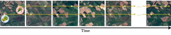
(a) Satellite image time series (SITS)
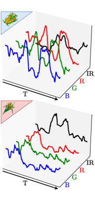
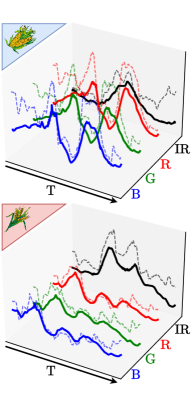
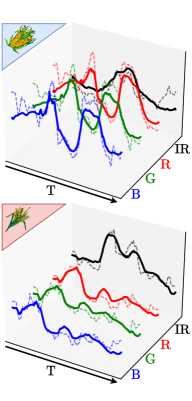
(b) Input	(c) Prototypes	(d) Recons.

Figure 1: Reconstructing pixel sequences from satellite image time series (SITS) through learned prototypes and transformations. Given a SITS (a), we reconstruct pixel-wise multi-spectral sequences using learned prototypes and transformations. Here, we show the RGB and IR spectral intensities over time for a corn () and a wheat () pixel sequence (b), along with their corresponding prototype before (c) and after (d) transformation.

With risks of food supply disruptions, constantly increasing energy needs, population growth and climate change, the threats faced by global agriculture production are plenty [42, 35]. Monitoring crop yield production, controlling vegetal health and growth, and optimizing crop rotations are among the essential tasks to be carried out at both national and global scales. Because regular ground-based surveys are challenging, remote sensing has very early on appeared as the most practical tool [23].

Thanks to public and commercial satellite launches such as ESA’s Sentinel constellation [12, 1], NASA’s Landsat [60] or Planet’s PlanetScope constellation [4, 55], Earth observation is now possible at both high temporal frequency and moderate spatial resolution, typically in the range of 10m/pixel. Sensed data can thus be processed as satellite image time series (SITS) at either the image or pixel level. In particular, several recent agricultural SITS datasets [28, 27, 59, 17, 47] make such data available to the machine learning community, mainly for improving crop type classification.

In this paper, we focus on methods approaching SITS segmentation as multivariate time series classification (MTSC) by considering multi-spectral pixel sequences as the data to classify. While this excludes some methods, such as [17] which explicitly leverages the extent of individual parcels, it enables us to extensively evaluate more general MTSC methods that have not yet been applied to agricultural SITS classification. We give particular attention to unsupervised methods as well as interpretability, which we believe would be appealing for extending results beyond well annotated geographical areas.

Our contributions are twofold. First, we benchmark approaches on four recent SITS datasets [28, 27, 59, 17] in both the supervised and unsupervised settings. State-of-the-art supervised methods [16, 54, 62] are typically complex and require vast amounts of labeled data, i.e., time series with accurate crop labels. We show that, while they provide strong accuracy boosts on datasets with limited domain gap between train and test data, they do not improve over the simple nearest centroid classification baseline on the more challenging DENETHOR [28] dataset. K-means clustering [33] and its variant [40, 63] using dynamic time warping (DTW) metric - instead of euclidean distance - are the strongest baselines [44] in the unsupervised setting.

Second, we adapt the deep transformation-invariant (DTI) clustering [36] to SITS classification by designing a transformation module corresponding to time warping. While deep unsupervised methods rely either on representation learning or pseudo-labeling, our method learns deformable prototypical sequences (Figure 1) by optimizing a reconstruction loss. Prototypes are multivariate time series, typically representing a type of crop, and that can be deformed to model intra-class variabilities. Following [31], we present results with prototypes learned with and without supervision, as extensions of the nearest centroid classifier [10] or the K-means clustering [33], depending on the case.

2 Related Work

We first review methods specifically designed for SITS classification which are typically supervised and may take as input complete images or individual pixel sequences. When each pixel sequence is considered independently, SITS classification can be seen as a specific case of MTSC, for which both supervised and unsupervised approaches exist, which we review next. Finally, we review transformation-invariant prototype-based classification approaches which we extend to SITS classification in this paper.

Supervised satellite image time series classification.

Deep networks for SITS classification either take individual pixel sequences [18, 16, 20, 2] or series of images [46, 39, 17] as input. While treating images as a whole may undeniably improves pattern learning for classification as the model can access spatial context information, we focus our work on pixel sequences, which allows us to present a simpler and less restrictive framework that can generalize better to various forms of input data. We evaluate our approach on four recent datasets of agricultural geospatial data [17, 28, 27, 59].

Supervised multivariate times series classification.

Methods achieving MTSC can be divided in two sub-groups: whole series-based techniques and feature-based techniques. Whole series-based methods includes nearest-neighbor search - where the closest neighbor is computed either using Euclidian distance [10] or DTW [52] - and prototype-based approaches that model a template for each class of the dataset [50, 51] and classify an input at inference by assigning it to the nearest prototype. Feature-based classifiers include bag-of-patterns methods [48, 49], shapelet-based techniques [30, 5] and deep encoders like 1D-CNNs [54, 22] or LSTMs [25, 62, 20].

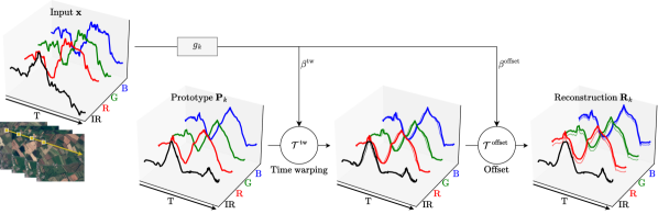
Figure 2: Overview of the method. Our method reconstructs a pixel-wise multi-spectral input sequence, extracted from a SITS, thanks to a prototype to which are successively applied a time warping and an offset. The parameters of these transformations are input-dependent and prototype-specific. The functions $g_{1:K}$ predicting the parameters of the transformations and the prototypes $\mathbf{P}_{1:K}$ can be learned with or without supervision.

Unsupervised multivariate time series classification.

The classical approach to multivariate time series clustering is to apply K-means [33] to the raw time series. DTW has been shown to improve upon K-means for time series clustering in the particular case of SITS [63, 40]. DTW is used during both steps of K-means: the assignment is performed under DTW and the centroids are updated as the DTW-barycenter averages of the newly formed clusters.

Approaches to multivariate time series clustering often work on improving the representation used by K-means. Methods either extract hand-crafted features [57, 43, 41] or apply principal component analysis [29, 53]. In [41], mean-shift [9] is used to segment the image into potential individual crops and K-means features are the means of the spectral bands and the smoothness, area and elongation of the obtained segments. [24] reproduces this multi-step scheme but instead (i) applies mean-shift segmentation to a feature map encoded by a 3D spatio-temporal deep convolutional autoencoder, (ii) takes the median of the spectral bands over a segment as a feature representation, and (iii) uses hierarchical clustering to classify each segment. Other deep approaches that perform unsupervised classification of time series either use pseudo-labels to train neural networks in a supervised fashion [19, 21] or focus on learning deep representations on which clustering can be performed with standards algorithms [15, 56]. DTIC [19] iteratively trains a TempCNN [39] with pseudo-labelling and performs K-means on the learned features to update the pseudo-labels.

Methods that perform deep unsupervised representation learning and clustering simultaneously [8, 61] are promising for time series classification. Although some recent works [15, 56] train supervised classifiers using these learned features on temporal data as input, to the best of our knowledge, no method designed for time series performs classification in a fully unsupervised manner.

Transformation-invariant prototype-based classification.

The DTI framework [36] jointly learns prototypes and prototype-specific transformations for each sample. Each prototype is associated with a transformation network, which predicts transformation parameters for every sample and thus enables the prototype to better reconstruct them. The resulting models can be used for downstream tasks such as classification [36, 31], few-shot segmentation [32] and multi-object instance discovery [37] and be trained with or without supervision. To the best of our knowledge, the DTI framework has never been applied to the case of time series, for which classifiers need to be invariant to some temporal distortions. Previous works bypass this concern using DTW to compare the samples to classify [40, 50] or by applying a transformation field to a selection of control points to distort the time series. Specific to agricultural time series, [38] leverages the fact that temperature is the main factor of temporal variations and uses thermal positional encoding of the temporal dimension to account for temperature change from a year (or location) to another. We use the DTI framework to instead learn the alignment of samples to the prototypes. [51] explores a similar idea for generic univariate time series, but, to the best of our knowledge, our paper is the first to perform both supervised and unsupervised transformation-invariant classification for agricultural satellite time series.

3 Method

In this section, we explain how we adapt the DTI framework [36] to pixel-wise SITS classification. First, we explain our model and network architecture (Sec. 3.1). Second, we present our training losses in the supervised and unsupervised cases and give implementation and optimization details (Sec. 3.2).

Notation.

We use bold letters for multivariate time series (e.g., $\mathbf{a}$, $\mathbf{A}$), brackets $[.]$ to index time series dimensions and we write $a_{1:N}$ for the set $\{a_{1},...,a_{n}\}$.

3.1 Model

Overview.

An overview of our model is presented in Figure 2. We consider a pixel time series $\mathbf{x}$ in $\mathbb{R}^{T\times C}$ of temporal length $T$ with $C$ spectral bands and we reconstruct it as a transformation of a prototypical time series. We will consider a set of $K$ prototypical time series $\mathbf{P}_{1:K}$, each one being a time series $\mathbf{P}_{k}\in\mathbb{R}^{T\times C}$ of same size as $\mathbf{x}$ and each intuitively corresponding to a different crop type.

We consider a family of multivariate time series transformations $\mathcal{T}_{\beta}:\mathbb{R}^{T\times C}\longrightarrow\mathbb{R}^{T\times C}$ parametrized by $\beta$. Our main assumption is that we can faithfully reconstruct the sequence $\mathbf{x}$ by applying to a prototype $\mathbf{P}_{k}$ a transformation $\mathcal{T}_{g_{k}(\mathbf{x})}$ with some input-dependent and prototype-specific parameters $g_{k}(\mathbf{x})$ .

We denote by $\mathbf{R}_{k}(\mathbf{x})\in\mathbb{R}^{T\times C}$ the reconstruction of the time series $\mathbf{x}$ obtained using a specific prototype $\mathbf{P}_{k}$ and the prototype-specific parameters $g_{k}(\mathbf{x})$:

$$\mathbf{R}_{k}\big{(}\mathbf{x}\big{)}=\mathcal{T}_{g_{k}(\mathbf{x})}\big{(}\mathbf{P}_{k}\big{)}.$$ (1)

Intuitively, a prototype corresponds to a type of crop (wheat, oat, etc) and a given input should be best reconstructed by the prototype of the corresponding class. For this reason, we want the transformations to only account for intra-class variability, which requires defining an adapted transformation model.

Transformation model.

We have designed a transformation model specific to SITS and based on two transformations: an offset along the spectral dimension and a time warping.

The ’offset’ transformation allows the prototypes to be shifted in the spectral dimension to best reconstruct a given input time series (Figure 3(a)). More formally, the deformation with parameters $\beta^{\text{offset}}$ in $\mathbb{R}^{C}$ applied to a prototype $\mathbf{P}$ can be written as:

$$\mathcal{T}^{\text{offset}}_{\beta^{\text{offset}}}\big{(}\mathbf{P}\big{)}=\beta^{\text{offset}}+\mathbf{P},$$ (2)

where the addition is to be understood channel-wise.

The ’time warping’ deformation aims at modeling intra-class temporal variability (Figure 3(b)) and is defined using a thin-plate spline [3] transformation along the temporal dimension of the time series. More formally, we start by defining a set of $M$ uniformly spaced landmark time steps $(t_{1},...,t_{M})^{T}$. Given $M$ target time steps $\beta^{\text{tw}}=(\beta^{\text{tw}}_{1},...,\beta^{\text{tw}}_{M})^{T}$, we denote by $h_{\beta^{\text{tw}}}$ the unique 1D thin-plate spline that maps each $t_{m}$ to $t_{m}^{\prime}=t_{m}+\beta^{\text{tw}}_{m}$. Now, given an input pixel time series $\mathbf{x}$ and $\beta^{\text{tw}}\in\mathbb{R}^{M}$, we define the time warping deformation applied to a prototype $\mathbf{P}$ as:

$$\mathcal{T}^{\text{tw}}_{\beta^{\text{tw}}}\big{(}\mathbf{P}\big{)}[t]=\mathbf{P}\big{[}h_{\beta^{\text{tw}}}(t)\big{]},$$ (3)

for $t\in[1,T]$. Note that the offset is time-independent and that the time warping is channel-independent.

To define our full transformation model, we compose these two transformations, which leads to reconstructions:

$$\mathbf{R}_{k}\big{(}\mathbf{x}\big{)}=\mathcal{T}^{\text{offset}}_{\beta^{\text{offset}}}\circ\mathcal{T}^{\text{tw}}_{\beta^{\text{tw}}}\big{(}\mathbf{P}_{k}\big{)}\text{, with }(\beta^{\text{offset}},\beta^{\text{tw}})=g_{k}(\mathbf{x}).$$ (4)

Architecture.

We implement the functions $g_{1:K}$ predicting the transformation parameters as a neural network composed of a shared encoder, for which we use the convolutional network architecture proposed by [58], and a final linear layer with $K\times(C+M)$ outputs followed by the hyperbolic tangent (tanh) function as activation layer. We interpret this output as $K$ sets of $(C+M)$ parameters for the transformations of the $K$ prototypes. By design, these transformation parameters take values in $[-1,1]$. This is adapted for the offset transformation since we normalize the time series before processing, but not for the time warping. We thus multiply the outputs of the network corresponding to the time warping parameters so that the maximum shift of the control time step corresponds to a week. We choose $M$ for each dataset so that we have a landmark time-step every month. In the supervised case, we choose $K$ equal to the number of crop classes in each dataset and we set $K$ to 32 in the unsupervised case.

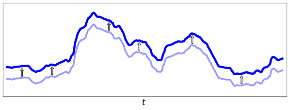
(a) Offset with $\beta^{\text{offset}}=0.3$

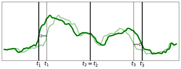
(b) Time warping with $M=3$, $\beta_{1}^{\text{tw}}=-7$, $\beta_{2}^{\text{tw}}=0$ and $\beta_{3}^{\text{tw}}=7$

Figure 3: Prototype deformations. We show the visual interpretations of our time series deformations. The offset deformation is time-independent and performed on each spectral band separately. On the other hand, time warping is channel-independent and achieved by translating landmark time-steps, allowing targeted temporal adjustments.

3.2 Losses and training

We learn the prototypes $\mathbf{P}_{1:K}$ and the deformation prediction networks $g_{1:K}$ by minimizing a mean loss on a dataset of $N$ multivariate pixel time series $\mathbf{x}_{1:N}$. We define this loss below in the supervised and unsupervised scenarios.

Unsupervised case.

In this scenario, our loss is composed of two terms. The first one is a reconstruction loss and corresponds to the mean squared error between the input time series and the transformed prototype that best reconstructs it for all pixels $\mathbf{x}$ of the studied dataset:

$$\mathcal{L}_{\text{rec}}(\mathbf{P}_{1:K},g_{1:K})=\frac{1}{NTC}\sum_{i=1}^{N}\underset{k}{\min}\Big{|}\Big{|}\mathbf{x}_{i}-\mathbf{R}_{k}(\mathbf{x}_{i})\Big{|}\Big{|}_{2}^{2}.$$ (5)

The second loss is a regularization term, which prevents high frequencies in the learned prototypes. Indeed, the time warping module allows interpolations between prototype values at consecutive time steps $t$ and $t+1$, and our network could thus use temporal shifts together with high-frequencies in the prototypes to obtain better reconstructions. To avoid these unwanted high-frequency artifacts, we add a total variation regularization [45]:

$$\mathcal{L}_{\text{tv}}(\mathbf{P}_{1:K})=\frac{1}{(KT-1)C}\sum_{k=1}^{K}\sum_{t=1}^{T-1}\Big{|}\Big{|}\mathbf{P}_{k}[t+1]-\mathbf{P}_{k}[t]\Big{|}\Big{|}_{2}.$$ (6)

The full training loss without supervision is thus:

$$\mathcal{L}_{\text{unsup}}(\mathbf{P}_{1:K},g_{1:K})=\mathcal{L}_{\text{rec}}(\mathbf{P}_{1:K},g_{1:K})+\lambda\mathcal{L}_{\text{tv}}(\mathbf{P}_{1:K}),$$ (7)

with $\lambda$ a scalar hyperparameter set to $0.01$ in all our experiments.

Supervised case.

In the supervised scenario, we choose $K$ as the true number of classes in the studied dataset, and set a one-to-one correspondence between each prototype and one class. We leverage this knowledge of the class labels to define two losses. Let $y_{i}\in\{1,...,K\}$ be the class label of input pixel $\mathbf{x}_{i}$. First, a reconstruction loss similar to (5) penalizes the mean squared error between an input and its reconstruction using the true-class prototype:

$$\mathcal{L}_{\text{rec\_sup}}(\mathbf{P}_{1:K},g_{1:K})=\frac{1}{NTC}\sum_{i=1}^{N}\Big{|}\Big{|}\mathbf{x}_{i}-\mathbf{R}_{y_{i}}(\mathbf{x})\Big{|}\Big{|}_{2}^{2}.$$ (8)

Second, in order to boost the discriminative power of our model, we add a contrastive loss [31] based on the reconstruction error:

$$\begin{split}&\mathcal{L}_{\text{cont}}(\mathbf{P}_{1:K},g_{1:K})=\\ &-\frac{1}{N}\sum_{i=1}^{N}\log\Bigg{(}\frac{\exp\big{(}-\Big{|}\Big{|}\mathbf{x}_{i}-\mathbf{R}_{y_{i}}(\mathbf{x})\Big{|}\Big{|}_{2}^{2}\big{)}}{\sum_{k=1}^{K}\exp\big{(}-\Big{|}\Big{|}\mathbf{x}_{i}-\mathbf{R}_{k}(\mathbf{x})\Big{|}\Big{|}_{2}^{2}\big{)}}\Bigg{)}.\end{split}$$ (9)

We also use the same total variation regularization as in the unsupervised case, and the full training loss under supervision is:

$$\begin{split}\mathcal{L}_{\text{sup}}(\mathbf{P}_{1:K},g_{1:K})=&\mathcal{L}_{\text{rec\_sup}}(\mathbf{P}_{1:K},g_{1:K})+\mu\mathcal{L}_{\text{tv}}(\mathbf{P}_{1:K})\\ &+\nu\mathcal{L}_{\text{cont}}(\mathbf{P}_{1:K},g_{1:K}),\end{split}$$ (10)

with $\mu$ and $\nu$ two hyperparameters equal to $0.01$ in all our experiments.

Optimization.

We use the ADAM [26] optimizer with a learning rate of $10^{-5}$. We train our model following a curriculum modeling scheme [14, 36]: we progressively increase the model complexity by first training without deformation, then adding the time warp deformation and finally the offset deformation. We add transformations when the mean accuracy does not increase in the supervised setting and, in the unsupervised setting, when the reconstruction loss does not decrease, after 1500 iterations. Note that the contrastive loss is only activated at the end of the curriculum in the supervised setting.

4 Experiments

4.1 Datasets

Dataset	Country	$T$	$C$	$K$	Train/Test shift	Satellite(s)	Daily	Split size (x $10^{6}$)
PASTIS [17]		406	10	19	Spat.	Sentinel 2	✗	7.3 $|$ 7.3 $|$ 7.3 $|$ 7.0 $|$ 7.1
TimeSen2Crop [59]		363	9	16	Spat.	Sentinel 2	✗	0.8 $|$ 0.1 $|$ 0.1
SA [27]		244	4	5	Spat.	PlanetScope	✓	60.1 $|$ 10.1 $|$ 32.0
DENETHOR [28]		365	4	9	Spat. & Temp.	PlanetScope	✓	20.6 $|$ 3.2 $|$ 22.8

Table 1: Comparison of studied datasets. The datasets we study cover different regions (France, Austria, South Africa and Germany). We distinguish between datasets where train and test splits differ only spatially (Spat.) and where they differ both spatially and temporally (Spat. & Temp.). Time series can have daily data (✓) or missing data (✗). Additionally, we report the length of the time series $T$, the number of spectral bands $C$ and the number of classes $K$. The last column shows the split sizes as train $|$ val $|$ test, except for PASTIS where we follow the 5-fold procedure described in [17] and we show the size of each of the folds.

We consider four recent open-source datasets on which we evaluate our method and multiple baselines. Details about these datasets can be found in Table 1.

PASTIS [17].

This dataset contains Sentinel-2 satellite patches within the French metropolitan area, acquired from September 1, 2018 to October 31, 2019. Each image time series contains a variable number of images that can show clouds and/or shadows. We pre-process the dataset and remove most of the cloudy/shadowy pixels using a classical thresholding approach on the blue reflectance [7]. We consider each of the pixels of the 2433 $128\times 128$ image time series as independent time series, except those corresponding to the ’void’ class, leading to $36$M times series. Each is labeled with one of 19 classes (including a background, i.e., non-agricultural class). We follow the same 5-fold evaluation procedure as described in [17], with at least 1km separating images from different folds to ensure distinct spatial coverage between them.

TimeSen2Crop [59].

This dataset is also built from Sentinel-2 satellite images, but covering Austrian agricultural parcels and acquired between September 3, 2017 and September 1, 2018. It does not provide images but directly $1$M pixel time series of variable lengths. We pre-process these time series by removing the time-stamps associated to the ’shadow’ and ’clouds’ annotations provided in the dataset. Each time series is labeled with one of 16 types of crops. We follow the same train/val/test splitting as in [59] where each split covers a different area in Austria.

SA [27].

This dataset is built from images from the PlanetScope constellation of Cubesats satellite covering agricultural areas in South Africa, and contains daily time series from April 1, 2017 to November 31, 2017. Acquisitions are fused using Planet Fusion to compensate for possible missing dates, clouds or shadows so that the provided data consists in clean daily image time series. The dataset contains 4151 single-field images time series from which we extract $102$M pixel time series. Each time series is labeled with one of 5 types of crops. We keep the same train/test splitting of the data and reserve 15% of the train set for validation purposes. We make sure that the obtained train and validation set do not have pixel time series extracted from the same field image.

DENETHOR [28].

This dataset is also built from Cubesats images but covers agricultural areas in Germany. The training set is built from daily time series acquired from January 1, 2018 to December 31, 2018, while the test set is built from time series acquired from January 1, 2019 to December 31, 2019. The time shift between train and test sets makes this dataset significantly more challenging than the three previous ones. Similar to SA, the dataset has been pre-processed to provide clean daily time series. It contains 4561 single-field images time series from which we extract $47$M independent pixel time series. Each time series is labeled with one of 9 types of crops. Again, we use the original splits of the data, with 15% of the training set kept for validation. All splits cover distinct areas in Germany.

Missing data.

Our method, as presented in Section 3, is designed for uniformly sampled constant-sized time series. While DENETHOR and SA time series have been pre-processed to obtain such regular data, PASTIS and TimeSen2Crop have at most a data point every 5 days due to a lower revisit frequency, and additional missing dates because of clouds or shadows. To handle such non-regularly sampled time series, we propose a simple interpolation scheme to transform raw time series into complete time series and an associated adaptation of our losses.

Let us consider a specific time series, acquired over a period of length $T$ but with missing data. We define the associated raw time series $\mathbf{x}_{\text{raw}}\in\mathbb{R}^{T\times C}$ by setting zero values for missing time steps and the associated binary mask $m_{\text{raw}}\in\{0,1\}^{T}$, equal to $0$ for missing time stamps and $1$ otherwise. We define the interpolated time series $\mathbf{x}$ extracted from $\mathbf{x}_{\text{raw}}$ and $m_{\text{raw}}$ through Gaussian filtering for $t\in[1,T]$ by:

$$\mathbf{x}[t]=\frac{1}{m[t]}\sum_{t^{\prime}=1}^{T}\mathcal{G}_{t,\sigma}[t^{\prime}]\cdot\mathbf{x}_{\text{raw}}[t^{\prime}],$$ (11)

with

$$\mathcal{G}_{t,\sigma}[t^{\prime}]=\exp\Big{(}-\frac{(t^{\prime}-t)^{2}}{2\sigma^{2}}\Big{)},$$ (12)

where $\sigma$ is a hyperparameter set to 7 days in our experiments. We also define the associated interpolated mask $m$ for $t\in[1,T]$ by:

$$m[t]=\sum_{t^{\prime}=1}^{T}\mathcal{G}_{t,\sigma}[t^{\prime}]\cdot m_{\text{raw}}[t^{\prime}],$$ (13)

for $t\in[1,T]$ and with the same hyperparameter $\sigma$.

Using directly this interpolated time series to compute our mean square errors would lead to large errors, because data might be missing for long time periods. Thus, we modify the losses $\mathcal{L}_{\text{rec}}$ and $\mathcal{L}_{\text{rec\_sup}}$ by replacing the reconstruction error between a time series $\mathbf{x}$ and reconstruction $\mathbf{R}$,

$$\frac{1}{TC}\Big{|}\Big{|}\mathbf{x}-\mathbf{R}\Big{|}\Big{|}_{2}^{2}=\frac{1}{C}\sum_{t=1}^{T}\frac{1}{T}\Big{|}\Big{|}\mathbf{x}[t]-\mathbf{R}[t]\Big{|}\Big{|}_{2}^{2},$$ (14)

in Equations (5) and (8) by a weighted mean squared error:

$$\frac{1}{C}\sum_{t=1}^{T}\frac{m[t]}{\sum_{t^{\prime}=1}^{T}m[t^{\prime}]}\Big{|}\Big{|}\mathbf{x}[t]-\mathbf{R}[t]\Big{|}\Big{|}_{2}^{2}.$$ (15)

This adapted loss gives more weight to time stamps $t$ corresponding to true data acquisitions.

4.2 Quantitative evaluation

We validate our approach in two setups: supervised (classification) and unsupervised (clustering). In this section, we first compare our method to top-performing supervised methods proposed in the literature for MTSC (Sec. 4.2.1). We then demonstrate that our method outperforms the K-means baseline on all four datasets (Sec. 4.2.2) thanks to the design choices for our time series deformations.

4.2.1 Time series classification

The purpose of this section is to benchmark classic and state-of-the-art MTSC methods for crop classification in SITS data. Results are summarized in Table 2, where the different methods are:

• NCC [13]. The nearest centroid classifier (NCC) assigns to a test sample the label of the closest class average time series using the Euclidean distance. We also report the extension of NCC with our method to add invariance to time warping and sequence offset, as well as adding our contrastive loss.

• 1NN [10] and 1NN-DTW [50]. The first nearest neighbor algorithm assigns to a test sample the label of its closest neighbor in the train set, with respect to a given distance. This algorithm is computationally costly and, since the datasets under study typically contain millions of pixel time series, we search for neighbors of test samples in a random 0.1% subset of the train set and report the average over 5 runs with different subsets. We evaluate the nearest neighbor algorithm using the Euclidean distance (1NN) as well as using the dynamic time warping (1NN-DTW) metric on the TimeSen2Crop dataset which is small enough to compute it in a reasonable time.

• MLSTM-FCN [25]. MLST-FCN is a two-branch neural network concatenating the ouputs of an LSTM and a 1D-CNN to better encode time series. We use a non-official PyTorch implementation of MLSTM-FCN.

• TapNet [62]. TapNet uses a similar architecture to MLST-FCN to learn a low-dimensional representation of the data. Additionally, [62] learns class prototypes in this latent space using the softmin of the euclidian distances of the embedding to the different class prototypes as classification scores. We use the official PyTorch implementation with default parameters.

• OS-CNN [54]. The Omni-Scale CNN is a 1D convolutional neural network that has shown ability to robustly capture the best time scale because it covers all the receptive filed sizes in an efficient manner. We use the official implementation with default parameters.

• MLP+LTAE [16]. The Lightweight Temporal Attention Encoder (LTAE) is an attention-based network. Used along with a Pixel Set Encoder (PSE) [18], LTAE achieves good performances on images. To adapt it to time series, we instead use a MLP as encoder. We refer to this method as MLP+LTAE and we use the official PyTorch implementation of LTAE.

• UTAE [18]. In addition to SITS methods, we also report the scores of U-net with Temporal Attention Encoder (UTAE) on PASTIS dataset. This method leverages complete (constant-size) images. Since it can learn from the spatial context of a given pixel this state-of-the-art image sequence segmentation approach is expected to perform better than pixel-based MTSC approaches and is reported for reference.

We provide two metrics for evaluating classification accuracy: overall accuracy (OA) and mean accuracy (MA). OA is computed as the ratio of correct and total predictions:

$$\text{OA}=\frac{\text{TP}+\text{TN}}{\text{TP}+\text{TN}+\text{FP}+\text{FN}},$$ (16)

where TP, TN, FP and FN correspond to true positive, true negative, false positive and false negative, respectively. MA is the class-averaged classification accuracy:

$$\text{MA}=\frac{1}{K}\sum_{k=1}^{K}\text{OA}(\{\mathbf{x}_{i}|y_{i}=k\}).$$ (17)

It is important to note that the datasets under consideration show a high degree of imbalance, making MA a more appropriate and informative metric for evaluating classification performance. For this reason, OA scores are shown in grey in Table 2, 3 and 4.

	#param	PASTIS		TimeSen2Crop		SA		DENETHOR
Method	(x1000)	OA$\uparrow$	MA$\uparrow$	OA$\uparrow$	MA$\uparrow$	OA$\uparrow$	MA$\uparrow$	OA$\uparrow$	MA$\uparrow$
UTAE [17]	$1\ 087$	$\mathbf{83.4}$	$\mathbf{77.7}$	—	—	—	—	—	—
MLP + LTAE [16]	$320$	$80.6$	$65.9$	$\mathbf{88.7}$	$80.9$	$67.4$	$\mathbf{63.7}$	$55.6$	$43.6$
OS-CNN [54]	$4\ 729$	$\mathbf{81.3}$	$68.1$	$87.9$	$81.2$	$64.6$	$60.3$	$49.0$	$39.2$
TapNet [62]	$1\ 882$	$77.4$	$\mathbf{69.5}$	$83.9$	$\mathbf{83.0}$	$\mathbf{69.4}$	$62.5$	$\mathbf{61.5}$	$\mathbf{60.6}$
MLSTM-FCN [25]	$490$	$44.4$	$10.9$	$58.7$	$44.0$	$56.1$	$47.9$	$58.2$	$48.3$
1NN-DTW [50]	$0$	—	—	$32.2$	$23.0$	—	—	—	—
1NN [10]	$0$	$65.8$	$40.1$	$43.9$	$35.0$	$60.7$	$54.9$	$56.7$	$48.2$
NCC [13]	$77$	$56.5$	$48.4$	$57.4$	$49.5$	$51.3$	$46.4$	$61.3$	$55.5$
$+$ time warping	$427$	$56.2$	$51.4$	$59.9$	$52.3$	$54.5$	$49.7$	$\mathbf{62.4}$	$56.4$
$+$ offset	$451$	$53.5$	$53.8$	$57.3$	$55.0$	$60.6$	$50.0$	$59.8$	$\mathbf{62.9}$
$+$ contrastive loss	$451$	$\mathbf{73.7}$	$\mathbf{59.1}$	$\mathbf{78.5}$	$\mathbf{70.5}$	$\mathbf{62.3}$	$\mathbf{54.9}$	$56.5$	$54.2$

Table 2: Performance comparison for classification on all datasets. We report for our method and competing methods, the number of trainable parameters (#param), the accuracy (OA) and the mean class accuracy (MA). We separate with a vertical line the DENETHOR dataset where train and test splits are acquired during different periods (right) from the others (left). 1NN-DTW is tested on TimeSen2Crop dataset only, due to the expensive cost of the algorithm. We separate results in 3 parts: the image level method UTAE, MTSC methods and NCC and its extension with our proposed method. We put in bold the best method in each of the 3 parts and underline the absolute best for each dataset.

Results on the DENETHOR dataset are qualitatively very different from the results on the other datasets. We believe this is because DENETHOR has train and test splits corresponding to two distinct years. We thus analyze it separately.

Results on PASTIS, TimeSen2Crop and SA.

As expected, since UTAE can leverage knowledge on the spatial context of each pixel, it achieves the best score on PASTIS dataset by $2.1\%$ in overall accuracy and $8.2\%$ in mean accuracy. Our improvements over the NCC method [13] - adding time warping deformation, offset deformations and contrastive loss (9) - consistently boost the mean accuracy (MA). The improvement obtained by adding transformation modeling comes from a better capability to model the data, as confirmed by the detailed results reported in the left part of Table 4, where one can see the reconstruction error (i.e. $\mathcal{L}_{\text{rec}}$) significantly decreases when adding these transformations. Note that on the contrary, adding the discriminative loss increase the accuracy at the cost of decreasing the quality of the reconstruction error. Our complete supervised approach outperforms both the nearest neighbor based methods and MLSTM-FCN. However, it is still significantly outperformed by top MTSC methods. This is not surprising, since these methods are able to learn complex embeddings that capture subtle signal variations, e.g. thanks to a temporal attention mechanism [16] or to multiple-sized receptive fields [54]. Note however that in doing so, they loose the interpretability of simpler approaches such as 1NN or NCC, which our method is designed to keep.

Results on DENETHOR.

Because the data we use is highly dependent on weather conditions, subsets acquired on distinct years follow significantly different distributions [28]. Because of their complexity, other methods struggle to deal with this domain shift. In this setting, our extension of NCC to incorporate specific meaningful deformations achieves better performances than all the other MTSC methods we evaluated. However, adding the contrastive loss significantly degrades the results. We believe this is again due to the temporal domain shift between train and test data. This analysis is supported by results reported in Table 4 which show that on the validation set of DENETHOR, which is sampled from the same year as the training data, adding the constrative loss significantly boost the results, similar to the other dataset. One can also see again on DENETHOR the benefits of modeling the deformations in term of reconstruction error. Note these results emphasize the need for more multi-year datasets to reliably evaluate the potential of automatic methods for practical crop segmentation scenarios, for which our deformation modeling approach seems to provide significant advantages.

4.2.2 Time series clustering

	#param	PASTIS		TimeSen2Crop		SA		DENETHOR
Method	(x1000)	OA$\uparrow$	MA$\uparrow$	OA$\uparrow$	MA$\uparrow$	OA$\uparrow$	MA$\uparrow$	OA$\uparrow$	MA$\uparrow$
K-means-DTW [40]	$520$	—	—	$40.5$	$26.8$	—	—	—	—
USRL [15]+K-means	$290$	$63.9$	$20.4$	$34.9$	$23.6$	$60.9$	$48.6$	$54.0$	$46.4$
DTAN [51]+K-means	$646$	$65.6$	$21.4$	$47.7$	$29.3$	$60.5$	$48.6$	$46.3$	$36.9$
K-means [6]	$520$	$69.0$	$29.8$	$49.5$	$32.5$	$61.9$	$47.8$	$57.2$	$48.5$
$+$ time warping	$1\ 209$	$\mathbf{69.1}$	$\mathbf{30.4}$	$\mathbf{52.3}$	$\mathbf{36.0}$	$\mathbf{64.1}$	$\mathbf{51.7}$	$57.6$	$51.1$
$+$ offset	$1\ 373$	$67.7$	$28.6$	$52.0$	$35.5$	$63.6$	$50.4$	$\mathbf{58.5}$	$\mathbf{52.6}$

Table 3: Performance comparison for clustering on all datasets. We report for our method and competing methods the number of trainable parameters (#param), the accuracy (OA) and the mean class accuracy (MA). K-means clustering is run with 32 clusters for all methods for fair comparison. We separate with a vertical line the DENETHOR datasets where train and test splits are acquired during different periods (right) from the others (left). K-means-DTW is tested on TimeSen2Crop dataset only, due to the expensive cost of the algorithm.

In this section, we demonstrate clear boosts provided by our method on the four SITS datasets we study. We compare our method to other clustering approaches applied on learned features or directly on the time series. Our results are summarized in Table 3 and the different methods are detailed below:

• K-means [6]. We apply the classic K-means algorithm on the multivariate pixel time series directly. Clustering is performed on all splits (train, val and test). Then we determine the most frequently occurring class in each cluster, considering training data only. The result is used as label for the entire cluster. We use the gradient descent version [6] K-means with empty cluster reassignment [8, 36].

• K-means-DTW [40]. The K-means algorithm is applied in this case with a dynamic time warping metric instead of the usual Euclidean distance. To this end, we use the differentiable Soft-DTW [11] version of DTW and its Pytorch implementation [34].

• USRL [15] + K-means. USRL is an encoder trained in an unsupervised manner to represent time series by a 320-dimensional vector. We train USRL on all splits of each dataset, then apply K-means in the feature space. We use the official implementation of USRL with default parameters.

• DTAN [51] + K-means. DTAN is an unsupervised method for aligning temporally all the time series of a given set. K-means is applied on data from all splits after alignment with DTAN. We use the official implementation of DTAN with default parameters.

We evaluate all methods with $K=32$ clusters.

Our method outperforms all the other baselines on the four datasets, always achieving the best mean accuracy. In particular, our time warping transformation appears to be the best way to handle temporal information when clustering agricultural time series. Indeed, DTAN+K-means leads to a significantly less accurate clustering than simple K-means. It confirms that temporal information is crucial when clustering agricultural time series: aligning temporally all the sequences of a given dataset leads to a loss of discriminative information. The same conclusion can be drawn from the results of K-means-DTW on TimeSen2Crop. In contrast, our time warping appears as constrained enough to both reach satisfying scores and account for the temporal diversity of the data.

Using an offset transformation on the spectral intensities consistently results in improved sample reconstruction using our prototypes, as demonstrated in Table 4. However, it only increases classification scores for DENETHOR. We attribute this improvement to the offset transformation’s ability to better handle the domain shift between the training and testing data on the DENETHOR dataset. The results on the other datasets suggest that this transformation accounts for more than just intra-class variability, leading to less accurate classification scores.

4.3 Qualitative evaluation

We show in Figure 4 our prototypes and how they are deformed to reconstruct a given input. For each class of the SA dataset, we show an input time series that has been correctly assigned to its corresponding prototype by our model trained with supervision but without $\mathcal{L}_{\text{cont}}$. We see that the inputs are best reconstructed by a prototype of their class. Looking at any of the columns, we see that prototypes of other classes can also be deformed to reconstruct a given input, but only to a certain extent. This confirms that the transformations considered are simple enough so that the reconstruction power of each prototype is limited, but powerful enough to allow the prototypes to adapt to their input.

Prototypes	Inputs	Reconstructions
Canola
​​​​ ​​	​​​​ ​​	​​​​ ​​
​​​​ ​​	​​​​ ​​	​​​​ ​​
​​​​ ​​	​​​​ ​​	​​​​ ​​
​​​​ ​​	​​​​ ​​	​​​​ ​​
​​​​ ​​	​​​​ ​​	​​​​ ​​
​​​​ ​​	​​​​ ​​	​​​​ ​​
​​​​ ​​	​​​​ ​​	​​​​ ​​
​​​​ ​​	​​​​ ​​	​​​​ ​​
​​​​ ​​	​​​​ ​​	​​​​ ​​
​​​​ ​​	​​​​ ​​	​​​​ ​​
​​​​ ​​	​​​​ ​​	​​​​ ​​
​​​​ ​​	​​​​ ​​	​​​​ ​​
​​​​ ​​	​​​​ ​​	​​​​ ​​
​​​​ ​​	​​​​ ​​	​​​​ ​​
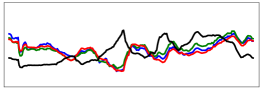
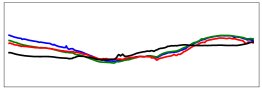
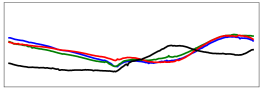
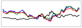
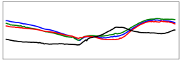
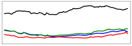
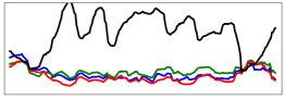
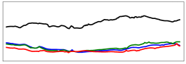
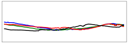
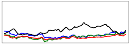
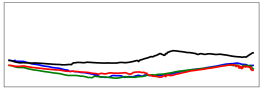
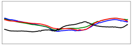
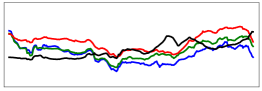
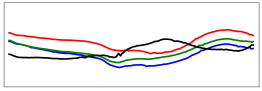
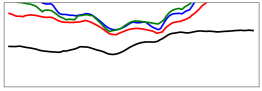
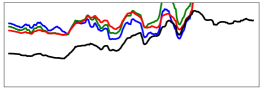
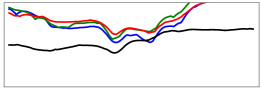
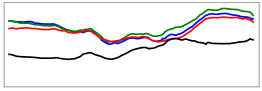
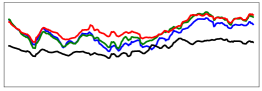
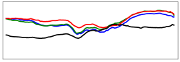
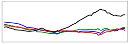
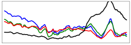
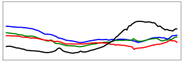
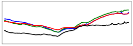
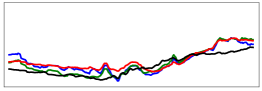
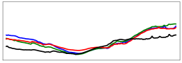
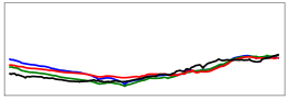
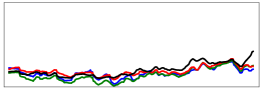
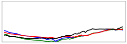
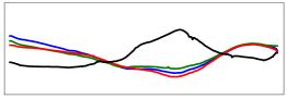
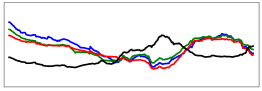
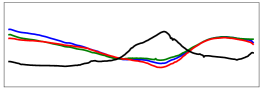
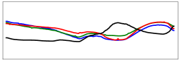
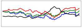
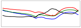
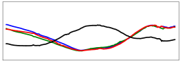
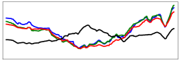
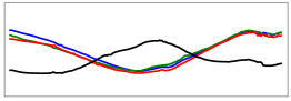
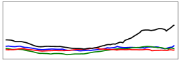
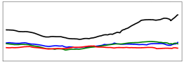
Small Grain Gazing
​​​​ ​​	​​​​ ​​	​​​​ ​​

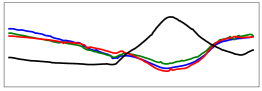
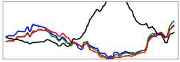
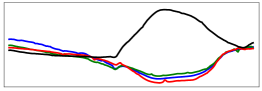
Figure 5: Learned prototypes on SA. We show the 32 prototypes learned on the SA dataset [27] (first column) in the unsupervised setting with time warping and offset deformations. For each prototype, we show an example time series of the corresponding class from the test set that is best reconstructed by it (second column) along with its reconstruction by our model (third column).

Figure 5 shows the 32 prototypes learned by our unsupervised model on SA, grouped by assigned label. For each prototype, we show an example input sample whose best reconstruction is obtained using this particular prototype and the obtained corresponding reconstruction. We see that prototypes are not equally assigned to classes, with class Canola having 14 prototypes when class Small Grain Gazing only has 1. This is due to the high imbalance of the classes in the datasets and different intra-class variabilities. Inside a class, different prototypes account for intra-class variability beyond what our deformations can model.

		Supervised						Unsupervised
		Val			Test			Train			Test
		OA$\uparrow$	MA$\uparrow$	$\mathcal{L}_{\text{rec}}\downarrow$	OA$\uparrow$	MA$\uparrow$	$\mathcal{L}_{\text{rec}}\downarrow$	OA$\uparrow$	MA$\uparrow$	$\mathcal{L}_{\text{rec}}\downarrow$	OA$\uparrow$	MA$\uparrow$	$\mathcal{L}_{\text{rec}}\downarrow$
PASTIS	Raw prototypes	$57.3$	$50.0$	$4.43$	$56.5$	$48.4$	$4.46$	$69.1$	$29.8$	$2.77$	$69.0$	$29.8$	$2.78$
	$+$ time warping	$56.8$	$53.7$	$4.00$	$56.2$	$51.4$	$4.04$	$\mathbf{69.2}$	$\mathbf{30.4}$	$2.53$	$\mathbf{69.1}$	$\mathbf{30.4}$	$2.53$
	$+$ offset	$55.0$	$55.7$	$\mathbf{2.57}$	$53.5$	$53.8$	$\mathbf{2.65}$	$67.8$	$28.5$	$\mathbf{1.91}$	$67.7$	$28.6$	$\mathbf{1.91}$
	$+$ $\mathcal{L}_{\text{cont}}$	$\mathbf{74.8}$	$\mathbf{61.3}$	$2.90$	$\mathbf{73.7}$	$\mathbf{59.1}$	$3.00$	—	—	—	—	—	—
TS2C	Raw prototypes	$57.4$	$51.2$	$4.89$	$57.4$	$49.5$	$4.36$	$56.2$	$34.2$	$3.52$	$49.5$	$32.5$	$3.56$
	$+$ time warping	$56.0$	$51.2$	$4.64$	$59.9$	$52.3$	$4.15$	$59.1$	$38.6$	$3.04$	$\mathbf{52.3}$	$\mathbf{36.0}$	$3.09$
	$+$ offset	$56.9$	$51.8$	$3.50$	$57.3$	$55.0$	$3.49$	$\mathbf{60.0}$	$\mathbf{39.3}$	$\mathbf{2.40}$	$52.0$	$35.5$	$\mathbf{2.53}$
	$+$ $\mathcal{L}_{\text{cont}}$	$\mathbf{74.5}$	$\mathbf{64.4}$	$\mathbf{3.46}$	$\mathbf{78.5}$	$\mathbf{70.5}$	$\mathbf{3.46}$	—	—	—	—	—	—
SA	Raw prototypes	$54.8$	$50.0$	$3.43$	$51.3$	$46.4$	$4.62$	$60.9$	$50.9$	$1.43$	$61.9$	$47.8$	$1.85$
	$+$ time warping	$57.5$	$53.9$	$2.93$	$54.5$	$49.7$	$4.13$	$62.2$	$53.1$	$1.03$	$\mathbf{64.1}$	$\mathbf{51.7}$	$1.46$
	$+$ offset	$63.5$	$58.0$	$\mathbf{1.34}$	$60.6$	$50.0$	$\mathbf{2.01}$	$\mathbf{63.7}$	$\mathbf{54.5}$	$\mathbf{0.67}$	$63.6$	$50.4$	$\mathbf{0.91}$
	$+$ $\mathcal{L}_{\text{cont}}$	$\mathbf{71.0}$	$\mathbf{64.7}$	$1.89$	$\mathbf{62.3}$	$\mathbf{54.9}$	$2.66$	—	—	—	—	—	—
DENETHOR	Raw prototypes	$68.3$	$58.0$	$3.89$	$61.3$	$55.5$	$4.58$	$63.8$	$52.8$	$2.67$	$57.2$	$48.5$	$2.41$
	$+$ time warping	$70.1$	$59.5$	$3.52$	$\mathbf{62.4}$	$56.4$	$4.21$	$64.8$	$54.0$	$2.23$	$57.6$	$51.1$	$2.01$
	$+$ offset	$77.3$	$64.9$	$\mathbf{2.39}$	$59.8$	$\mathbf{62.9}$	$\mathbf{3.55}$	$\mathbf{66.2}$	$\mathbf{56.3}$	$\mathbf{1.70}$	$\mathbf{58.5}$	$\mathbf{52.6}$	$\mathbf{1.56}$
	$+$ $\mathcal{L}_{\text{cont}}$	$\mathbf{85.1}$	$\mathbf{75.5}$	$3.00$	$56.5$	$54.2$	$4.35$	—	—	—	—	—	—

Table 4: Detailed evaluation of our method. We show the impact of the increasing complexity of our modeling for reconstruction and accuracy on all datasets in both the supervised and unsupervised settings. Note that learning raw prototypes boils down to the NCC method [10] in the supervised setting and to the K-means algorithm [33] in the unsupervised setting.

		Inputs
		Wheat	Barley	Lucerne / Medics	Canola	Small Grain Gazing
		​​	​​	​​	​​	​​
Prototypes	​​	​​​​ ​​	​​​​ ​​	​​​​ ​​	​​​​ ​​	​​​​ ​​
	Wheat	$\mathcal{L}_{\text{rec}}=0.134$	$\mathcal{L}_{\text{rec}}=0.494$	$\mathcal{L}_{\text{rec}}=0.609$	$\mathcal{L}_{\text{rec}}=0.575$	$\mathcal{L}_{\text{rec}}=0.542$
	​​	​​​​ ​​	​​​​ ​​	​​​​ ​​	​​​​ ​​	​​​​ ​​
	Barley	$\mathcal{L}_{\text{rec}}=0.145$	$\mathcal{L}_{\text{rec}}=0.456$	$\mathcal{L}_{\text{rec}}=0.568$	$\mathcal{L}_{\text{rec}}=0.685$	$\mathcal{L}_{\text{rec}}=0.589$
	​​	​​​​ ​​	​​​​ ​​	​​​​ ​​	​​​​ ​​	​​​​ ​​
	Lucerne / Medics	$\mathcal{L}_{\text{rec}}=0.388$	$\mathcal{L}_{\text{rec}}=0.578$	$\mathcal{L}_{\text{rec}}=0.501$	$\mathcal{L}_{\text{rec}}=0.666$	$\mathcal{L}_{\text{rec}}=0.704$
	​​	​​​​ ​​	​​​​ ​​	​​​​ ​​	​​​​ ​​	​​​​ ​​
	Canola	$\mathcal{L}_{\text{rec}}=0.302$	$\mathcal{L}_{\text{rec}}=0.960$	$\mathcal{L}_{\text{rec}}=0.822$	$\mathcal{L}_{\text{rec}}=0.249$	$\mathcal{L}_{\text{rec}}=0.852$
	​​	​​​​ ​​	​​​​ ​​	​​​​ ​​	​​​​ ​​	​​​​ ​​
	Small Grain Gazing	$\mathcal{L}_{\text{rec}}=0.153$	$\mathcal{L}_{\text{rec}}=0.510$	$\mathcal{L}_{\text{rec}}=0.563$	$\mathcal{L}_{\text{rec}}=0.478$	$\mathcal{L}_{\text{rec}}=0.537$

Figure 4: Reconstructions from different prototypes. We show the reconstructions of input samples (columns) from SA [27] by learned prototypes (lines) in the supervised setting without $\mathcal{L}_{\text{cont}}$. Selected prototypes (frames) correspond to the lowest reconstruction error.

5 Conclusion

We have presented an approach to learning invariance to transformations relevant for time series using deep learning, and demonstrated how it can be used to perform both supervised and unsupervised pixel-based classification of agricultural SITS. We perform our analysis on four recent public datasets with diverse characteristics and covering different countries. Our method significantly improves the performance of NCC and K-means on all datasets, while keeping their interpretability. We show it improves the state of the art on the DENETHOR dataset for classification, and on all datasets for clustering. Additionally, we provide a benchmark of MTSC classification approaches for agricultural SITS classification.

Prototypes	Inputs	Reconstructions
Wheat
​​​​ ​​	​​​​ ​​	​​​​ ​​
​​​​ ​​	​​​​ ​​	​​​​ ​​
​​​​ ​​	​​​​ ​​	​​​​ ​​
​​​​ ​​	​​​​ ​​	​​​​ ​​
​​​​ ​​	​​​​ ​​	​​​​ ​​
​​​​ ​​	​​​​ ​​	​​​​ ​​
​​​​ ​​	​​​​ ​​	​​​​ ​​
Barley
​​​​ ​​	​​​​ ​​	​​​​ ​​
​​​​ ​​	​​​​ ​​	​​​​ ​​
​​​​ ​​	​​​​ ​​	​​​​ ​​
​​​​ ​​	​​​​ ​​	​​​​ ​​
Lucerne / Medics
​​​​ ​​	​​​​ ​​	​​​​ ​​
​​​​ ​​	​​​​ ​​	​​​​ ​​
​​​​ ​​	​​​​ ​​	​​​​ ​​
​​​​ ​​	​​​​ ​​	​​​​ ​​
​​​​ ​​	​​​​ ​​	​​​​ ​​
​​​​ ​​	​​​​ ​​	​​​​ ​​

Acknowledgments.

The work of MA was partly supported by the European Research Council (ERC project DISCOVER, number 101076028). JP was supported in part by the Louis Vuitton/ENS chair on artificial intelligence and the French government under management of Agence Nationale de la Recherche as part of the Investissements d’avenir program, reference ANR19-P3IA0001 (PRAIRIE 3IA Institute). This work was granted access to the HPC resources of IDRIS under the allocation 2021-AD011013067 made by GENCI. We thank Antoine Guédon for inspiring discussions; Tom Monnier, Romain Loiseau, Ricardo Garcia Pinel, Théo Bodrito, Yannis Siglidis and Loïc Landrieu for manuscript feedback and constructive insights.

References

- [1] Josef Aschbacher, Masami Onoda, and Oran R Young. ESA’s Earth Observation Strategy and Copernicus, pages 81–86. Springer Singapore, Singapore, 2017.
- [2] Mariana Belgiu and Ovidiu Csillik. Sentinel-2 cropland mapping using pixel-based and object-based time-weighted dynamic time warping analysis. Remote Sensing of Environment, 204:509–523, 2018.
- [3] Fred L. Bookstein. Principal warps: Thin-plate splines and the decomposition of deformations. IEEE Transactions on pattern analysis and machine intelligence, 11(6):567–585, 1989.
- [4] Christopher Boshuizen, James Mason, Pete Klupar, and Shannon Spanhake. Results from the planet labs flock constellation. AIAA/USU Conference on Small Satellites, 2014.
- [5] Aaron Bostrom and Anthony Bagnall. Binary shapelet transform for multiclass time series classification. In International conference on big data analytics and knowledge discovery, pages 257–269. Springer, 2015.
- [6] Leon Bottou and Yoshua Bengio. Convergence properties of the k-means algorithms. Advances in neural information processing systems, 7, 1994.
- [7] Francois-Marie Breon and Stéphane Colzy. Cloud Detection from the Spaceborne POLDER Instrument and Validation against Surface Synoptic Observations. Journal of Applied Meteorology, 38(6):777–785, June 1999.
- [8] Mathilde Caron, Piotr Bojanowski, Armand Joulin, and Matthijs Douze. Deep clustering for unsupervised learning of visual features. In Proceedings of the European conference on computer vision (ECCV), pages 132–149, 2018.
- [9] Dorin Comaniciu and Peter Meer. Mean shift: A robust approach toward feature space analysis. IEEE Transactions on pattern analysis and machine intelligence, 24(5):603–619, 2002.
- [10] Thomas Cover and Peter Hart. Nearest neighbor pattern classification. IEEE transactions on information theory, 13(1):21–27, 1967.
- [11] Marco Cuturi and Mathieu Blondel. Soft-dtw: a differentiable loss function for time-series. In International Conference on Machine Learning, pages 894–903. PMLR, 2017.
- [12] Matthias Drusch, Umberto Del Bello, Sébastien Carlier, Olivier Colin, Veronica Fernandez, Ferran Gascon, Bianca Hoersch, Claudia Isola, Paolo Laberinti, Philippe Martimort, et al. Sentinel-2: Esa’s optical high-resolution mission for gmes operational services. Remote sensing of Environment, 120:25–36, 2012.
- [13] Richard O Duda, Peter E Hart, and David G Stork. Pattern classification and scene analysis, volume 3. Wiley New York, 1973.
- [14] Jeffrey L Elman. Learning and development in neural networks: The importance of starting small. Cognition, 48(1):71–99, 1993.
- [15] Jean-Yves Franceschi, Aymeric Dieuleveut, and Martin Jaggi. Unsupervised scalable representation learning for multivariate time series. Advances in neural information processing systems, 32, 2019.
- [16] Vivien Sainte Fare Garnot and Loic Landrieu. Lightweight temporal self-attention for classifying satellite images time series. In International Workshop on Advanced Analytics and Learning on Temporal Data, pages 171–181. Springer, 2020.
- [17] Vivien Sainte Fare Garnot and Loic Landrieu. Panoptic segmentation of satellite image time series with convolutional temporal attention networks. In Proceedings of the IEEE/CVF International Conference on Computer Vision, pages 4872–4881, 2021.
- [18] Vivien Sainte Fare Garnot, Loic Landrieu, Sebastien Giordano, and Nesrine Chehata. Satellite image time series classification with pixel-set encoders and temporal self-attention. In Proceedings of the IEEE/CVF Conference on Computer Vision and Pattern Recognition, pages 12325–12334, 2020.
- [19] Wenqi Guo, Weixiong Zhang, Zheng Zhang, Ping Tang, and Shichen Gao. Deep temporal iterative clustering for satellite image time series land cover analysis. Remote Sensing, 14(15):3635, 2022.
- [20] Dino Ienco, Raffaele Gaetano, Claire Dupaquier, and Pierre Maurel. Land cover classification via multitemporal spatial data by deep recurrent neural networks. IEEE Geoscience and Remote Sensing Letters, 14(10):1685–1689, 2017.
- [21] Jawad Iounousse, Salah Er-Raki, Ahmed El Motassadeq, and Hassan Chehouani. Using an unsupervised approach of probabilistic neural network (pnn) for land use classification from multitemporal satellite images. Applied Soft Computing, 30:1–13, 2015.
- [22] Hassan Ismail Fawaz, Benjamin Lucas, Germain Forestier, Charlotte Pelletier, Daniel F Schmidt, Jonathan Weber, Geoffrey I Webb, Lhassane Idoumghar, Pierre-Alain Muller, and François Petitjean. Inceptiontime: Finding alexnet for time series classification. Data Mining and Knowledge Discovery, 34(6):1936–1962, 2020.
- [23] Christopher O Justice and Inbal Becker-Reshef. Report from the workshop on developing a strategy for global agricultural monitoring in the framework of group on earth observations (geo). In Avaliable online: http://www. fao. org/gtos/igol/docs/meeting-reports/07-geo-ag0703-workshop-report-nov07. pdf (accessed on 11 June 2015), volume 595, 2007.
- [24] Ekaterina Kalinicheva, Jérémie Sublime, and Maria Trocan. Unsupervised satellite image time series clustering using object-based approaches and 3d convolutional autoencoder. Remote Sensing, 12(11):1816, 2020.
- [25] Fazle Karim, Somshubra Majumdar, Houshang Darabi, and Samuel Harford. Multivariate lstm-fcns for time series classification. Neural Networks, 116:237–245, 2019.
- [26] Diederik P Kingma and Jimmy Ba. Adam: A method for stochastic optimization. ICLR, 2015.
- [27] Lukas Kondmann, Sebastian Boeck, Rogerio Bonifacio, and Xiao Xiang Zhu. Early crop type classification with satellite imagery-an empirical analysis. ICLR 3rd Workshop on Practical Machine Learning in Developing Countries, 2022.
- [28] Lukas Kondmann, Aysim Toker, Marc Rußwurm, Andres Camero Unzueta, Devis Peressuti, Grega Milcinski, Nicolas Longépé, Pierre-Philippe Mathieu, Timothy Davis, Giovanni Marchisio, et al. Denethor: The dynamicearthnet dataset for harmonized, inter-operable, analysis-ready, daily crop monitoring from space. In Thirty-fifth Conference on Neural Information Processing Systems Datasets and Benchmarks Track, 2021.
- [29] Hailin Li. Multivariate time series clustering based on common principal component analysis. Neurocomputing, 349:239–247, 2019.
- [30] Jason Lines, Luke M Davis, Jon Hills, and Anthony Bagnall. A shapelet transform for time series classification. In Proceedings of the 18th ACM SIGKDD international conference on Knowledge discovery and data mining, pages 289–297, 2012.
- [31] Romain Loiseau, Baptiste Bouvier, Yann Teytaut, Elliot Vincent, Mathieu Aubry, and Loïc Landrieu. A model you can hear: Audio identification with playable prototypes. ISMIR, 2022.
- [32] Romain Loiseau, Tom Monnier, Mathieu Aubry, and Loïc Landrieu. Representing shape collections with alignment-aware linear models. In 2021 International Conference on 3D Vision (3DV), pages 1044–1053. IEEE, 2021.
- [33] J MacQueen. Classification and analysis of multivariate observations. In 5th Berkeley Symp. Math. Statist. Probability, pages 281–297, 1967.
- [34] Mehran Maghoumi, Eugene Matthew Taranta, and Joseph LaViola. Deepnag: Deep non-adversarial gesture generation. In 26th International Conference on Intelligent User Interfaces, pages 213–223, 2021.
- [35] C. Mbow, C. Rosenzweig, L. G. Barioni, T. G. Benton, M. Herrero, M. Krishnapillai, E. Liwenga, P. Pradhan, M. G. Rivera-Ferre, T. Sapkota, F. N. Tubiello, and Y. Xu. Food security. Intergovernmental Panel on Climate Change, 2019.
- [36] Tom Monnier, Thibault Groueix, and Mathieu Aubry. Deep transformation-invariant clustering. Advances in Neural Information Processing Systems, 33:7945–7955, 2020.
- [37] Tom Monnier, Elliot Vincent, Jean Ponce, and Mathieu Aubry. Unsupervised layered image decomposition into object prototypes. In Proceedings of the IEEE/CVF International Conference on Computer Vision, pages 8640–8650, 2021.
- [38] Joachim Nyborg, Charlotte Pelletier, and Ira Assent. Generalized classification of satellite image time series with thermal positional encoding. In Proceedings of the IEEE/CVF Conference on Computer Vision and Pattern Recognition (CVPR) Workshops, pages 1392–1402, June 2022.
- [39] Charlotte Pelletier, Geoffrey I Webb, and François Petitjean. Temporal convolutional neural network for the classification of satellite image time series. Remote Sensing, 11(5):523, 2019.
- [40] François Petitjean, Jordi Inglada, and Pierre Gançarskv. Clustering of satellite image time series under time warping. In 2011 6th International Workshop on the Analysis of Multi-temporal Remote Sensing Images (Multi-Temp), pages 69–72. IEEE, 2011.
- [41] François Petitjean, Camille Kurtz, Nicolas Passat, and Pierre Gançarski. Spatio-temporal reasoning for the classification of satellite image time series. Pattern Recognition Letters, 33(13):1805–1815, 2012.
- [42] Alexander Y. Prosekov and Svetlana A. Ivanova. Food security: The challenge of the present. Geoforum, 91:73–77, 2018.
- [43] Jebu J Rajan and Peter JW Rayner. Unsupervised time series classification. Signal processing, 46(1):57–74, 1995.
- [44] Antonio Jesús Rivera, María Dolores Pérez-Godoy, David Elizondo, Lipika Deka, and María José del Jesus. A preliminary study on crop classification with unsupervised algorithms for time series on images with olive trees and cereal crops. In International Workshop on Soft Computing Models in Industrial and Environmental Applications, pages 276–285. Springer, 2020.
- [45] Leonid I Rudin, Stanley Osher, and Emad Fatemi. Nonlinear total variation based noise removal algorithms. Physica D: nonlinear phenomena, 60(1-4):259–268, 1992.
- [46] Marc Rußwurm and Marco Körner. Convolutional lstms for cloud-robust segmentation of remote sensing imagery. arXiv preprint arXiv:1811.02471, 2018.
- [47] Marc Rußwurm, Charlotte Pelletier, Maximilian Zollner, Sébastien Lefèvre, and Marco Körner. Breizhcrops: A time series dataset for crop type mapping. International Archives of the Photogrammetry, Remote Sensing and Spatial Information Sciences ISPRS (2020), 2020.
- [48] Patrick Schäfer. The boss is concerned with time series classification in the presence of noise. Data Mining and Knowledge Discovery, 29(6):1505–1530, 2015.
- [49] Patrick Schäfer and Ulf Leser. Multivariate time series classification with weasel+ muse. arXiv preprint arXiv:1711.11343, 2017.
- [50] Skyler Seto, Wenyu Zhang, and Yichen Zhou. Multivariate time series classification using dynamic time warping template selection for human activity recognition. In 2015 IEEE symposium series on computational intelligence, pages 1399–1406. IEEE, 2015.
- [51] Ron A Shapira Weber, Matan Eyal, Nicki Skafte, Oren Shriki, and Oren Freifeld. Diffeomorphic temporal alignment nets. Advances in Neural Information Processing Systems, 32, 2019.
- [52] Mohammad Shokoohi-Yekta, Jun Wang, and Eamonn Keogh. On the non-trivial generalization of dynamic time warping to the multi-dimensional case. In Proceedings of the 2015 SIAM international conference on data mining, pages 289–297. SIAM, 2015.
- [53] Ashish Singhal and Dale E Seborg. Clustering multivariate time-series data. Journal of Chemometrics: A Journal of the Chemometrics Society, 19(8):427–438, 2005.
- [54] Wensi Tang, Guodong Long, Lu Liu, Tianyi Zhou, Michael Blumenstein, and Jing Jiang. Omni-scale CNNs: a simple and effective kernel size configuration for time series classification. In International Conference on Learning Representations, 2022.
- [55] Planet Team. Planet application program interface: In space for life on earth. San Francisco, CA, 2017:40, 2017.
- [56] Sana Tonekaboni, Danny Eytan, and Anna Goldenberg. Unsupervised representation learning for time series with temporal neighborhood coding. arXiv preprint arXiv:2106.00750, 2021.
- [57] Xiaozhe Wang, Kate A Smith, and Rob J Hyndman. Dimension reduction for clustering time series using global characteristics. In International Conference on Computational Science, pages 792–795. Springer, 2005.
- [58] Zhiguang Wang, Weizhong Yan, and Tim Oates. Time series classification from scratch with deep neural networks: A strong baseline. In 2017 International joint conference on neural networks (IJCNN), pages 1578–1585. IEEE, 2017.
- [59] Giulio Weikmann, Claudia Paris, and Lorenzo Bruzzone. Timesen2crop: A million labeled samples dataset of sentinel 2 image time series for crop-type classification. IEEE Journal of Selected Topics in Applied Earth Observations and Remote Sensing, PP:1–1, 04 2021.
- [60] C. E. Woodcock, R. Allen, M. Anderson, A. Belward, R. Bindschadler, W. Cohen, F. Gao, S. N. Goward, D. Helder, E. Helmer, R. Nemani, L. Oreopoulos, J. Schott, Prasad S. Thenkabail, E. F. Vermote, James E. Vogelmann, M. A. Wulder, and R. Wynne. Free access to landsat imagery. Science, 320(5879):1011–, 2008.
- [61] Asano YM., Rupprecht C., and Vedaldi A. Self-labelling via simultaneous clustering and representation learning. In International Conference on Learning Representations, 2020.
- [62] Xuchao Zhang, Yifeng Gao, Jessica Lin, and Chang-Tien Lu. Tapnet: Multivariate time series classification with attentional prototypical network. In Proceedings of the AAAI Conference on Artificial Intelligence, volume 34, pages 6845–6852, 2020.
- [63] Zheng Zhang, Ping Tang, Lianzhi Huo, and Zengguang Zhou. Modis ndvi time series clustering under dynamic time warping. International Journal of Wavelets, Multiresolution and Information Processing, 12(05):1461011, 2014.