The Fundamental Patterns of Sea Surface Temperature

Abstract

For over 40 years, remote sensing observations of the Earth’s oceans have yielded global measurements of sea surface temperature (SST). With a resolution of approximately 1 km, these data trace physical processes like western boundary currents, cool upwelling at eastern boundary currents, and the formation of mesoscale and sub-mesoscale eddies. To discover the fundamental patterns of SST on scales smaller than 10 km, we developed an unsupervised, deep contrastive learning model named Nenya. We trained Nenya on a subset of 8 million cloud-free cutout images ($\sim 80\times 80$ km²) from the MODerate-resolution Imaging Spectroradiometer (MODIS) sensor, with image augmentations to impose invariance to rotation, reflection, and translation. The 256-dimension latent space of Nenya defines a vocabulary to describe the complexity of SST and associates images with like patterns and features. We used a dimensionality reduction algorithm to explore cutouts with a temperature interval of $\Delta T=0.5-1$ K, identifying a diverse set of patterns with temperature variance on a wide range of scales. We then demonstrated that SST data with large-scale features arise preferentially in the Pacific and Atlantic Equatorial Cold Tongues and exhibit a strong seasonal variation, while data with predominantly sub-mesoscale structure preferentially manifest in western boundary currents, select regions with strong upwelling, and along the Antarctic Circumpolar Current. We provide a web-based user interface to facilitate the geographical and temporal exploration of the full MODIS dataset. Future efforts will link specific SST patterns to select dynamics (e.g., frontogenesis) to examine their distribution in time and space on the globe.

I Introduction

Decades of infrared (IR) observations made from satellite-borne sensors have been used to generate twice-daily (clouds permitting), global SST fields. While dependent upon the specific satellite sensor examined, as well as the level of processing applied, IR measurements nominally have spatial resolutions of $1$ km and temperature resolutions of several tenths Kelvin. Moreover, the swath widths of these sensors typically range from $1000$ to $2500$ km, permitting resolution of both mesoscale (horizontal scales of $30$-$200$ km) and sub-mesoscale ocean phenomena (horizontal scales of $1$-$50$ km). One notes the two length-scales overlap, in part because of the varying radius of deformation with latitude leading to different ranges for each throughout the literature. Examples of mesoscale phenomena include strong western boundary current systems such as the Gulf Stream, Kuroshio, and Aghulhas Currents, upwelling systems along eastern boundaries such as the California and Benguela Current Systems, tropical instability waves, large-scale eddies and/or baroclinic Rossby waves. Examples of sub-mesoscale processes include finer-scale fronts, filaments, and eddies that often result from stirring and straining by the mesoscale currents, and consequent instabilities that take place at these locations [1, 2]. In summary, IR satellite-derived measurements yield powerful datasets for exploring the physical properties and processes of our ocean over a broad range of spatial and temporal scales.

Impressively, one notes that data from even a single sensor, such as the MODIS dataset, satisfies most characteristics of so-called “big data.” For example, the Level-2 (L2) SST archive of the processed Aqua MODIS data stream ($2003$-$2021$, inclusive) comprises over 2 million individual 5-minute granules totalling over 20 TB. While much of these data have been probed by human investigations, the dataset far exceeds one’s capacity for an analysis by visual inspection alone. Moreover, the scope of this dataset poses computational challenges, both in terms of storage and processing resources. Yet, these hurdles are surmountable with modern approaches tailored to big data including cloud storage and modern-day machine learning (ML) techniques.

With this as background and armed with the MODIS dataset and ML tools, we are motivated to study SST patterns across the global ocean and over long time-periods to address the following questions. What are the fundamental patterns and characteristics of SST imagery? When and where do these patterns and characteristics manifest? And, ultimately, what do these patterns reflect about the underlying dynamics?

Our approach is to develop and apply ML techniques originally introduced for natural images (e.g., cats, dogs). By modifying and extending their application to SST imagery (in itself a class of natural images), we may perform novel investigations of the global ocean.

In an earlier study [3], we constructed and applied a probabilistic autoencoder (PAE) [4] nicknamed Ulmo to nighttime MODIS L2 SST data. The primary goals of this effort were to construct a massive dataset for exploration ($\sim 12,000,000$ thumbnails or “cutouts” of dimension $\approx 125\times 125$ km²) and to identify outliers from the full dataset (i.e., unusual phenomena at the ocean surface). The PAE is an unsupervised ML model which first encodes each cutout into a reduced-dimension latent space (the autoencoder). One then generates probabilistic statements on the cutout distribution, specifically the likelihood of a given cutout occurring within the full distribution reported as a log-likelihood (LL) metric.

After calculating the LL metric for $\sim 12,000,000$ cutouts, [3] showed that the majority of outlier patterns occur within previously known mesoscale eddying regions of the ocean, such as western boundary currents. While this result may have been anticipated by those familiar with physical oceanography, it verified the efficacy of unsupervised ML techniques applied to these massive SST datasets. On the other hand, the Ulmo LL metric fails to capture the full complexity of SST imagery–i.e., data with nearly identical LL may arise from distinctly different SST patterns associated with distinct physical processes. This limitation motivates the introduction of a new ML algorithm in this manuscript.

To further address our motivating questions, we build a new model – nicknamed Nenya – built on the unsupervised ML algorithm termed self-supervised (or contrastive) learning [5, 6, 7, 8, 9, 10, 11]. This deep learning approach was developed to generate associations amongst imagery with similar characteristics while separating them from data with contrasting nature. In the process, one may explore the diversity of patterns/scenes/etc. that occur within a massive imagery dataset (e.g., [12]). Regarding the ocean, this algorithm offers the opportunity to describe the fundamental patterns of SST fields without introducing rigid rules-based or statistical metrics that may predispose the outcome. Furthermore, it is straightforward afterward to apply any such metric to gain physical insight into the results.

II Data and Basic Metrics

II-A The Cutout Sample

In this manuscript we analyze the nighttime L2 SST Aqua MODIS dataset (https://oceancolor.gsfc.nasa.gov/data/aqua/) for the period 2003-2021 inclusive. Our approach to data extraction and pre-processing follow the procedures described in [3]. Specifically, we first generate patches with a size of approximately ${128\times 128}$ pixel² that are at least $96\%$ clear, land-free and of good quality. This is a stricter clear criterion than the $95\%$ clear criterion adopted in [3] as subsequent work has identified spurious results from improperly masked clouds or poor in-painting applied to images with $>\sim 5$% cloud coverage. We consider this to be the best trade-off between sample size and quality for the analysis presented here.

The patches were drawn randomly from the MODIS granules, restricted to lie within 480 pixels of nadir (to maintain $\sim 1$-km resolution) and required to have less than 50% overlap. By allowing for partial overlap, we generate more ‘views’ of a given field.

We then pre-process each patch by: (i) in-painting the bad (flagged) pixels; (ii) median filtering with a 3-pixel window in the along-track direction; (iii) resizing the patch to a ${64\times 64}$ pixel² cutout using the local mean of each $2\times 2$ region; and (iv) subtracting the mean temperature to produce an SST anomaly (i.e., SSTa) cutout. Table I lists a small set of the $\approx 8,000,000$ cutouts resulting from the parent sample; the full table is available online.

II-B LL and $\Delta T$

To build physical intuition for the results that follow, we introduce several metrics to describe the individual cutouts. Two of these metrics detailed in this sub-section are the Ulmo LL metric briefly described in the introduction and the temperature range $\Delta T$  defined as the difference in $90$th and $10$th percentiles of the anomaly (SSTa) distribution: $\Delta T\equiv T_{90}-T_{10}$ where $T_{N}$ denotes the $N^{th}$-percentile.

For each cutout we calculate the LL metric using the Ulmo PAE of [3]. Conceptually, the LL metric describes the relative occurrence of a given image within the ensemble distribution. Here, the distribution is constructed from the set of latent vectors derived from a deep-learning autoencoder designed to capture the features and patterns of SST imagery. To formally calculate LL, the latent space of the autoencoder outputs is transformed to a 512-dimension Gaussian manifold with a normalizing flow. The LL metric is then the sum of the log probability from the 512 Gaussians and the log of the determinant of the transformation. These give the normalization of the LL distribution [13].

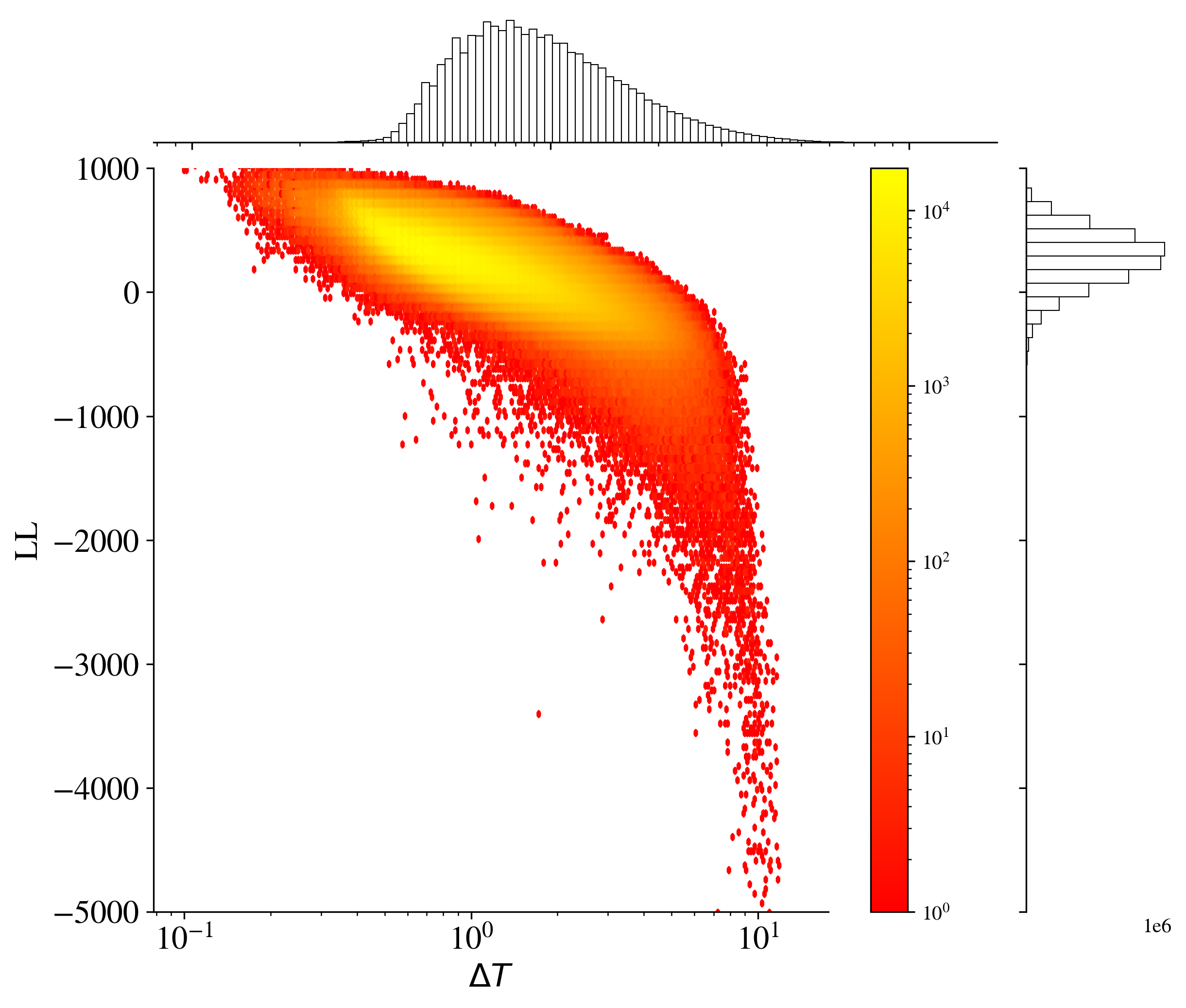
Figure 1: 2D histogram of the distribution of the LL metric vs. temperature range $\Delta T$, with the color proportional to the log of the counts in each bin. The two distributions are strongly correlated, with the highest $\Delta T$ exhibiting the lowest LL values. The marginal distributions are shown as simple histograms. While the LL distribution is well-described by a Gaussian, it does exhibit an asymmetric tail to very low values which are the extreme outliers of the dataset [3].

During their analysis, [3] discovered that the LL values of the cutouts correlate strongly with the temperature range. Put simply, cutouts with high $\Delta T$ are rare and yield lower LL values on average. We have calculated and tabulated $\Delta T$ for all of the cutouts (Table I), recovering a LogNormal distribution after allowing for a shift and scale,

$$p(\Delta T^{\prime})=\frac{1}{\sigma_{\Delta T}\Delta T^{\prime}\sqrt{2\pi}}\,\exp\left(-\frac{\ln^{2}\Delta T^{\prime}}{2\sigma_{\Delta T}^{2}}\right)$$ (1)

$\Delta T^{\prime}=(\Delta T-l_{\Delta T})/S_{\Delta T}$ finding $\sigma_{\Delta T}\approx 0.58$, $l_{\Delta T}\approx 0.1$, and $S_{\Delta T}\approx 0.83$. In comparison, the LL distribution is well-described by a Gaussian with mean $\bar{x}_{\rm LL}\approx 270$ and standard deviation $\sigma_{\rm LL}\approx 227$, albeit with a long tail to very low values that define the outlier sample of [3].

Figure 1 shows the LL vs. $\Delta T$ bivariate distribution; this reveals the strong correlation; e.g., cutouts with high $\Delta T$ exhibit the lowest LL. Despite the correlation, one should not over-interpret Figure 1 to conclude that the LL metric is solely tracking $\Delta T$ and therefore could be replaced by it. First, the relationship is not strict; there is a wide range of LL values at a given $\Delta T$. Furthermore, one expects a correlation with LL for any simple metric that describes the features in the imagery. However, no single metric can fully describe the complexity of SST imagery. Stated differently, the complexity of SST imagery belies any single, simple statistic – including the LL measure of our previous work. This motivates, in part, the application of an alternative, deep learning technique. As important, we found that the latent space of Ulmo did not group together cutouts with similar patterns. This too motivates the contrastive learning model adopted here.

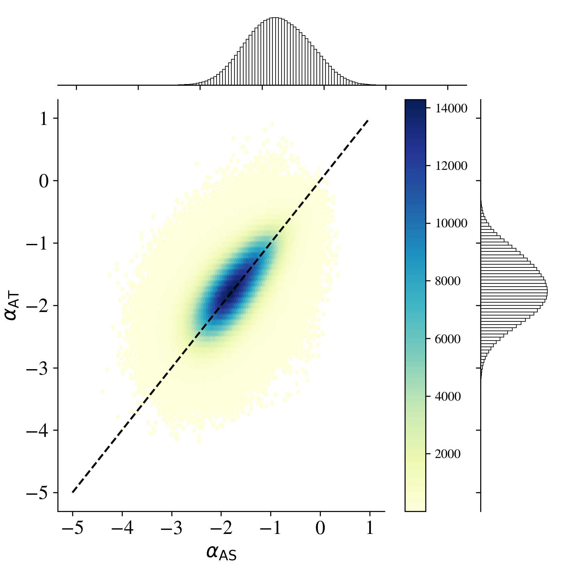
Figure 2: Bivariate distribution of the along-scan spectral slope $\alpha_{\rm AS}$ versus the along-track $\alpha_{\rm AT}$, each determined from the portion of the spectra for wavelengths between 12 and 50 km. Typical uncertainties in the measurements are one to several tenths (fitting error only). We find that $>99\%$ of the cutouts have $\alpha_{\rm AS}$ and $\alpha_{\rm AT}$ within one $\sigma$ of the estimated error from the 1-to-1 line, indicating their values are highly correlated. The good correspondence between the $\alpha_{\rm AS}$ and $\alpha_{\rm AT}$ implies isotropic motions within the ocean on these physical scales.

II-C Slopes of the Power Spectrum

Another metric often used to describe structure in SST fields is the slope $\alpha$ of the 1D power spectrum; i.e., the slope of the energy in wavenumber space. When estimated over fine horizontal scales, such as sub-mesoscales ($1-50$ km), the slope can be descriptive of underlying turbulent processes. For example, classical quasi-geostrophic (QG) turbulence predicts a spectral slope of $\alpha=-3$, surface quasi-geostrophic (SQG) turbulence predicts $\alpha=-5/3$, and an internal-wave continuum predicts $\alpha=-2$ (i.e., for scales less than 10 km and flatter otherwise) [14, 15, 16].

For the cutouts analyzed here, the smallest scales are expected to be dominated by instrument noise. Therefore, we focus the analysis on larger scales ($\lambda\approx 12-50$ km), which corresponds to the upper end of wavelengths associated with sub-mesoscale processes (depending on latitude). Focusing on this range also mitigates, to some extent, contributions to the spectral power at smaller scales due to the multi-detector nature of MODIS. Note, however, that a wavelength of $12$ km nominally resolves two eddy-like anomalies of opposite sign, each with radii of $3$ km. Since the mixed layer deformation radius of sub-mesoscale anomalies typically exceeds $3$ km, this resolves most sub-mesoscale phenomena except perhaps those at polar latitudes.

For each cutout, we determine ensemble averaged power spectra independently for the along-scan (AS) and along-track (AT) directions. Specifically, for each row (or column) of the cutout, we detrend the data with a linear fit and subtract the mean. We then calculate the fast fourier transform for each row/column and ensemble average the results by row/column. This signal is median filtered with a window of 5 pixels and a power-law is fit to the resultant power spectrum with related uncertainty. We refer to these slopes as $\alpha_{\rm AS}$ and $\alpha_{\rm AT}$ for the AS and AT directions, respectively.

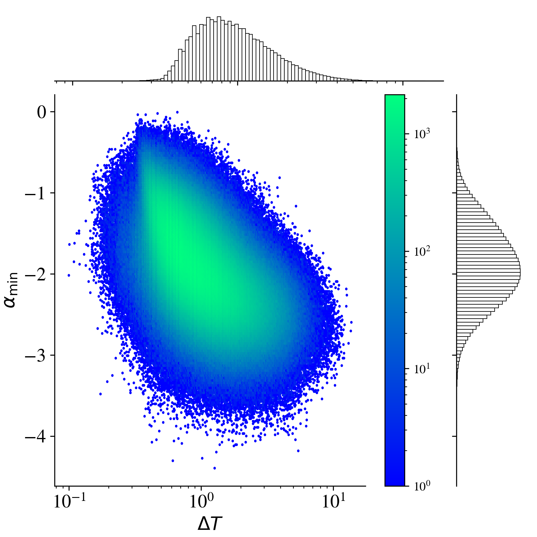
Figure 3: 2D histogram of the characterstic slope $\alpha_{\rm min}$ of each cutout vs. $\Delta T$. Regions of the ocean with larger temperature range also tend to exhibit a steeper power spectrum on $\sim 10-50$km scales, albeit with substantial scatter.

We applied this algorithm to all of the cutout images to calculate $\alpha_{\rm AS}$ and $\alpha_{\rm AT}$ independently (Table I) and also to estimate their uncertainties. Figure 2 plots the two slopes against one another. The marginal distributions of $\alpha_{\rm AS}$ and $\alpha_{\rm AT}$ are well described by Gaussians with nearly identical mean and standard deviations: $\bar{x}_{\alpha}\approx-1.74$, $\sigma_{\alpha}\approx 0.5$. Furthermore, we find the slopes for a given cutout agree within uncertainty for the overwhelming majority of cases (i.e., $99\%$ fall within one $\sigma$ of the mean). This suggests a high degree of isotropy within the dataset.

In the following, we characterize each cutout by a single spectral slope $\alpha_{\rm min}\equiv\min(\alpha_{\rm AS},\alpha_{\rm AT})$. Figure 3 shows this quantity versus $\Delta T$, revealing a correlation but with large scatter. Given Figure 1, one notes the $\alpha_{\rm min}$ is also correlated with LL  with the most negative $\alpha_{\rm min}$ (largest in magnitude) cutouts having preferentially lower LL (as one would expect).

III Methodology

III-A Overview

Recently, several simple yet powerful self-supervised learning (SSL) frameworks have been proposed to learn useful representations (latents) from high dimensional data sets. This includes so-called contrastive losses which maximize the “similarity” of the views from the same data samples in the latent space [5, 6, 7, 8, 9, 10, 11]. In our work, we apply the SimCLR framework to analyze the preprocessed cutouts ($64\times 64$ pixel² arrays) from the MODIS granules by designing task-dependent augmentations based on our domain knowledge of SST data. The latents obtained by our model are, as designed, a transformation-invariant representation of the SST data. We then study structure in the latent space by projecting into a two-dimensional vector space using a Uniform Manifold Approximation and Projection (UMAP) [17]. The reader is also encouraged to study the methodology developed by [18] using the scattering transform [19].

III-B An Introduction to SimCLR

SimCLR is an efficient but simple self-supervised learning model in which a base neural encoder is used to transform the augmented input data point to a latent vector $\tilde{\mathbf{z}}^{(i)}$. By minimizing the contrastive loss, an essential representation can be extracted [7]. The contrastive loss function defined for an augmented sample pair $\{\tilde{\mathbf{z}}^{(i)},\tilde{\mathbf{z}}^{(i^{\prime})}\}$ is given by:

$$\text{loss}_{i,j}=-\text{sim}(\tilde{\mathbf{z}}^{(i)},\tilde{\mathbf{z}}^{(j)})/\tau+\log{\sum_{k:k\neq i}^{2m}}\exp{(\text{sim}(\tilde{\mathbf{z}}^{(i)},\tilde{\mathbf{z}}^{(k)})/\tau)},$$ (2)

where $\text{sim}(\tilde{\mathbf{z}}^{(i)},\tilde{\mathbf{z}}^{(j)})$ is defined as the dot-product similarity of the latent pair $\{\tilde{\mathbf{z}}^{(i)},\tilde{\mathbf{z}}^{(j)}\}$, namely the output of the neural encoder, and $\tau$ is a hyper-parameter used to fine-tune the amplitude of the similarity. In essence, the contrastive loss (2) is just the rescaled similarity of the sample pair with a batch normaliziation penalty term.

For our model, we use ResNet-50 [20] as the encoder because unsupervised learning favors models with larger capacity [8]. We do not employ a projection head, and the latents generated by the encoder are passed directly to the contrastive loss function, without additional nonlinear transformation. The advantage of discarding the projection head is that a reasonable similarity can be defined for the latents obtained by the encoder during the evaluation step. After some experimentation, we have set the dimensionality of the latent space to 256.

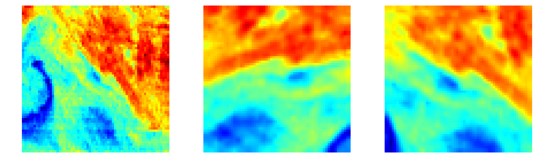
Figure 4: The left panel is the ‘raw’ cutout input to the augmentation module and the other two images are a pair of augmented samples. The first (center image) was randomly flipped about the vertical axis and then rotated by $\approx 320$ deg and jittered by 5 pixels vertically. The second (right image) was not flipped, was rotated by $\approx 18$ deg and jittered by 2 pixels horizontally and vertically. Each augmented image was then cropped by the inner $40\times 40$ pixel², resized to $64\times 64$ pixel² and demeaned.

III-C Augmentations

The random augmentation module is crucial for model performance and affects the nature of the patterns captured in the latent space. After experimenting with standard augmentations intended for natural images, we refined based on the following domain considerations: invariance to (i) rotation, (ii) translation, and (iii) reflection. The reason for the first consideration is that the MODIS L2 data product is not oriented parallel to either the zonal or meridional directions. Moreover, while there may be scientific motivations for preserving orientation when analyzing SSTa fields more generally, the north-south gradient in solar insolation and in beta has little impact on the gradient in SST at the scales of interest here ($<80$ km). This is supported by Figure 2. The reason for the second consideration is that we desired a description of the SST patterns that is insensitive to small spatial shifts. That is, viewing the region offset by, for example, $10$ km typically results in a similar pattern. Finally, the impetus for the third consideration is that we suspect a reflection or “mirror image” of the original cutout should capture all of the same information. As an aside, we also considered inverting the SSTa field (i.e., turning warm to cold), but did not do so in the end since some dynamic features have a physical preference (e.g., mesoscale currents are generally warmer than the surrounding waters).

With these considerations in mind, we imposed the following augmentations in this order:

• Random Flip: We randomly flip the image in each dimension with a 50% probability (e.g., a 25% probability of no alteration).

• Random Rotation: We rotate the cutouts with random angles which are uniformly sampled from $\theta=[0,2\pi]$. The new image maintains $64\times 64$ pixel² with data rotated ‘off’ now lost and otherwise empty regions imputed with 0 values.

• Random Jitter and Crop: We randomly select a new image center uniformly offset from the original by up to 5 pixels in each dimension. We crop the original image around the translated center to $40\times 40$ pixel² to eliminate the inclusion of the zero-filled portions introduced by the rotation. Last, we resize the cropped image back to the original grid size of $64\times 64$ pixel².

• Demean: The final image is demeaned.

Figure 4 shows a representative cutout and two of its randomly augmented samples. These were randomly flipped, rotated and jittered, and then cropped to the inner $40\times 40$ pixel², resized to $64\times 64$ pixel² and demeaned. Our SSL model, which operates solely on augmented images, learned to recognize these as similar and to distinguish their underlying patterns from those of other cutouts.

III-D Training and Evaluation

For training of the model, we randomly selected 600,000 cutouts from the full set. For validation, we randomly selected another 150,000 cutouts. With $4$ GPUs, we train Nenya with a batch size of 256. To monitor the contrastive lost on the validation set, we find that after $\approx 5$ epochs of training, the model learns good representations of the training data set. SSL models benefit from bigger batch sizes; our experimentation showed good performance for sizes of 256 or more.

In Fig. 5, we show the learning curves for the Nenya model in the training and validation process. Learning loss decreases rapidly with training batch number suggesting that the model converges well.

We then evaluated all 21 years of MODIS cutouts, generating and recording a unique 256-dimension latent vector for each. These constitute the learned representations of the fundamental SST patterns of the imagery on scales $\leq 80$ km.

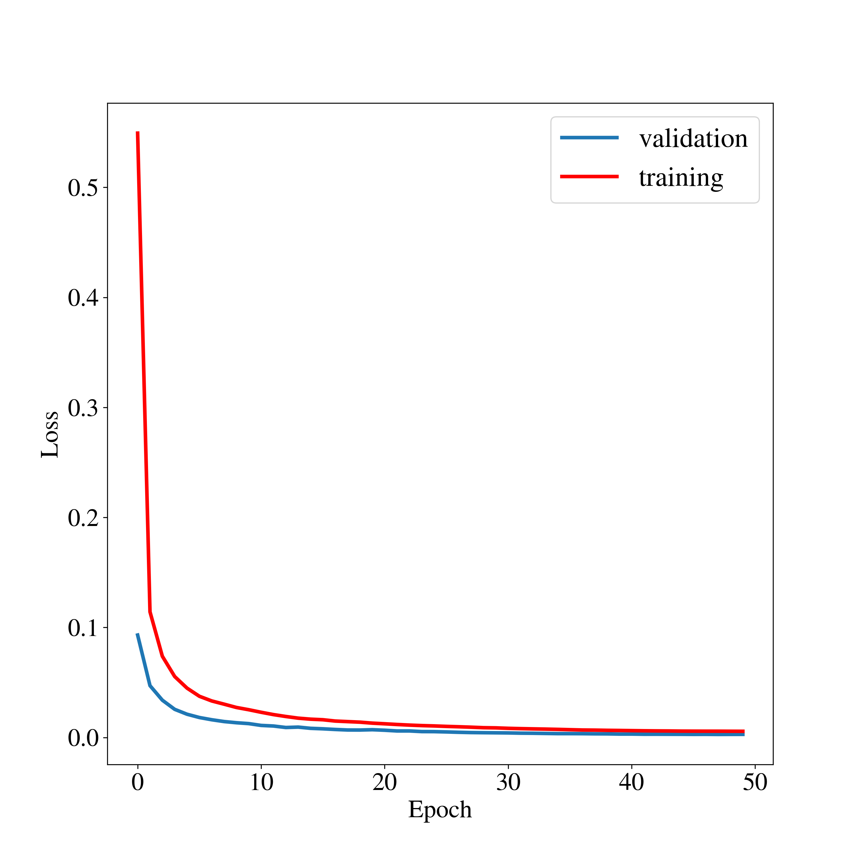
Figure 5: Learning curves (batch losses) for the training set (red) and validation set (blue) for our SSL model. The model achieves a low loss after $\approx 5$ epochs and has effectively converged after $\sim 20$.

III-E UMAP Dimensionality Reduction

While the latent vectors encode the features characterizing the SST patterns, it is difficult as humans to visualize and explore this 256-dimension latent space. Therefore, we have implemented the UMAP algorithm to further reduce the latent space to two dimensions ($U_{0},U_{1}$). We adopt the default parameters of the UMAP package [21] throughout.

We emphasize that neither of the parameters $U_{0},U_{1}$ need to have a direct, physical meaning or analogue. These are only statistical in nature, although they are tuned to separate the latent vector space and therefore track the fundamental patterns of SST imagery. Only the 256 dimension latent vectors are the full model representation of the underlying patterns–i.e., the two-dimensions of this UMAP are (by design) a limited representation of the full complexity. Nevertheless, we find that by applying the UMAP to a series of $\Delta T$ sub-samples that we describe a majority of the diversity within the dataset. The following section explores the outputs of this procedure and also their scientific implications.

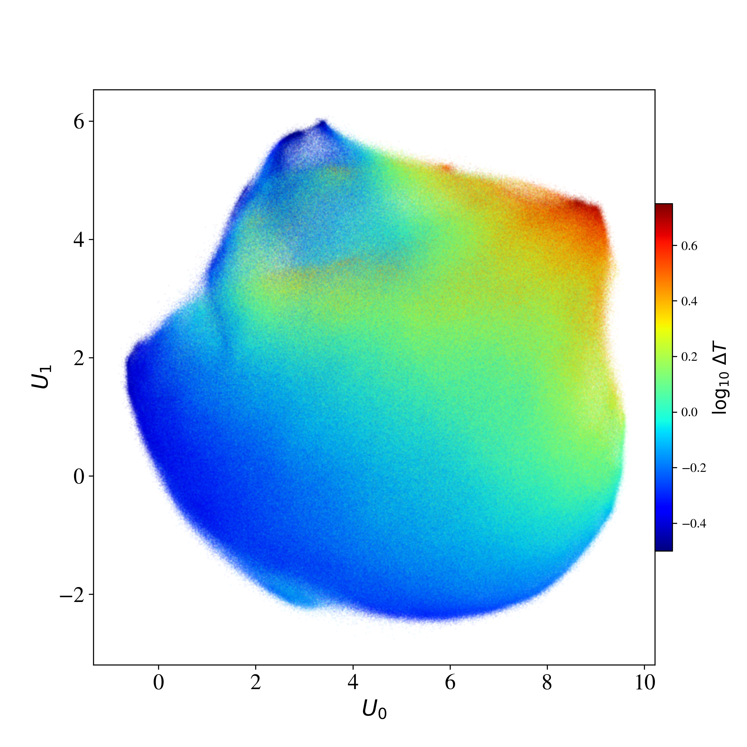
Figure 6: UMAP two-dimensional manifold description of the latent-vector space (256-dimensions) which represents the fundamental SST patterns. Each cutout is shown as a dot in the space, color-coded by $\log_{10}\Delta T$ of the cutout.

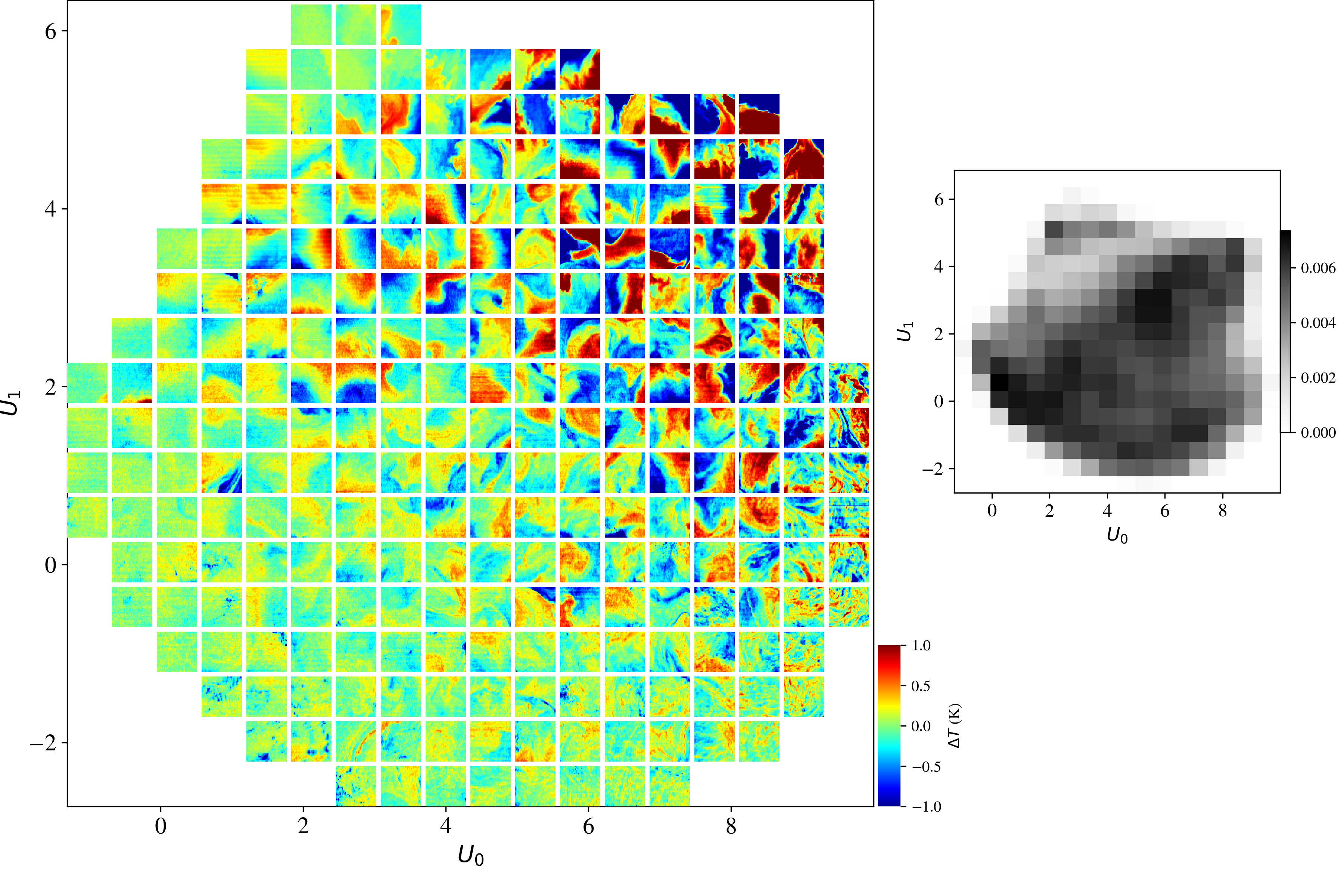
Figure 7: Gallery of cutouts, each one selected at random from a gridded $U_{0},U_{1}$ space for the full dataset.The data show increasing structure and complexity as one transitions from the lower left ($U_{0},U_{1}\approx[0,-1]$) to the upper right of the domain. Along this same direction the average $\Delta T$ is increasing, i.e., this embedding is especially sensitive to the cutout $\Delta T$. The gray histogram on the right describes the relative frequency of cutouts at each location in the UMAP domain.

IV Results

The previous section described the deep learning methodology introduced to analyze the MODIS L2 dataset. Specifically, the Nenya model was trained to associate images with similar SST patterns on scales of $\approx 80\times 80$ km² and smaller, while separating these from dissimilar images. The resulting 256-dimension latent space therefore represents a new method or vocabulary for describing SST imagery on sub-mesoscales. This section examines a portion of the vocabulary describing the rich complexity of SST imagery. To facilitate the exploration, we map the 256-dimension latent space to a reduced basis (two dimensions) for the full dataset and subsets in $\Delta T$.

IV-A Full Sample

We begin by examining the full sample, applying the UMAP algorithm to all of the $\approx 8,000,000$ latent vectors. Figure 6 shows the reduction of SST patterns into two dimensions for the full set of imagery, color-coded by $\log_{10}\Delta T$. The relatively uniform distribution indicates the SST imagery exhibits a smooth continuum of patterns and features as opposed to “clusters” of discrete classes. Furthermore, by coloring the data by $\Delta T$, we emphasize that this property is a dominant “axis” in separating the SST imagery (here oriented at $\sim 45^{\circ}$ to the $U_{0},U_{1}$ axes). The strong $\Delta T$ dependence is relatively obvious in hindsight; having removed the first moment in SST (the mean), the second moment (variance) remains a principle characteristic of each SSTa cutout. And while $\Delta T$ has physical significance for the ocean (e.g., high values preferentially arise in dynamically active regions), we wish to discriminate the patterns based on finer features. These are captured in the full 256-latent space and we access them in the following section by sub-dividing the full sample into $\Delta T$ intervals and then reducing each sub-sample with its own UMAP algorithm.

Before proceeding, we further examine the UMAP results for the full dataset via a gallery of representative images. We have gridded the $U_{0},U_{1}$ space and selected a random cutout from within each grid cell; these are plotted in Figure 7. As designed, Nenya has effectively separated the SST imagery by their patterns. Qualitatively, the data is highly uniform in the lower left region of the UMAP space $(U_{0},U_{1}\approx 0,-1)$ and one observes increasing complexity as one moves away from this “origin”. Greatest structure is evident at high $U_{0},U_{1}$ values, with patterns characterized by water masses of high positive and negative SSTa separated by a sharp front. These are likely associated with strong ocean currents, such as the Gulf Stream, Kuroshio, and Antarctic Circumpolar Current, regions of relatively large changes in shallow bathymetry often encountered near the edge of the continental shelf and in vertically stratified regions with strong winds such as off the Isthmus of Tehuantepec.

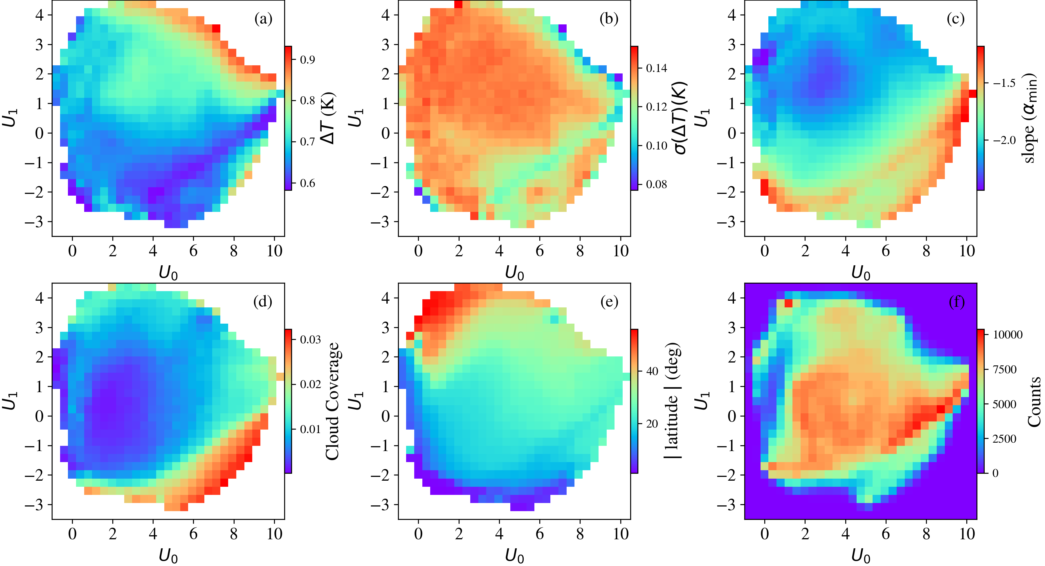
Figure 8: Binned evaluations in the UMAP embedding for properties of the cutout subset with $\Delta T=0.5-1\,{\rm K}$. Panels (a), (c), (d), and (e) show the median value of $\Delta T$ (with a linear color scale because of the relatively small temperature range compared with the log₁₀ scale used for Figure 6), $\alpha_{\rm min}$, cloud coverage, and the absolute latitude of the cutouts respectively. Panel (b) presents the standard deviation in $\Delta T$ and panel (f) records the number of cutouts in each bin.

IV-B The Fundamental Patterns of SST

In the previous sub-section, we showed that reducing the full set of latent vectors to two dimensions with a UMAP embedding primarily separated the SST patterns by $\Delta T$. While informative, this does not express well the great diversity within the dataset. Therefore, we proceeded to generate a unique UMAP embedding of the latent space for sub-samples of the cutouts separated by $\Delta T$. Specifically, we measure $\Delta T$ from the inner $40\times 40$ pixel² regions of each cutout which corresponds to the regions augmented by the Nenya model (see $\S$ III-C). We then consider $\Delta T$ bins as follows:

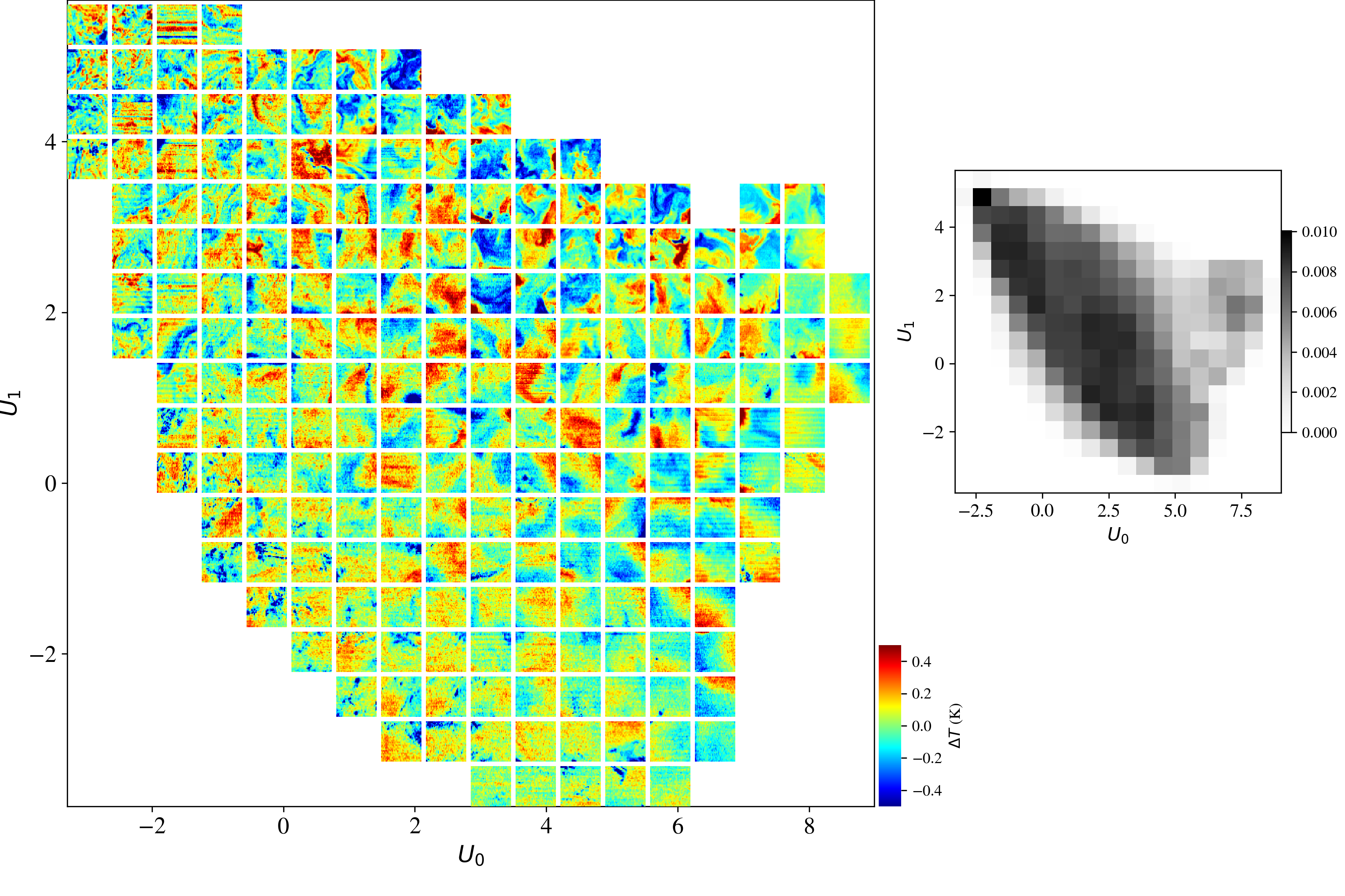
Figure 17: Same as Figure 7 but for the UMAP embedding of the $\Delta T=0-0.5\,{\rm K}$ sub-set of cutouts.

1. ${\Delta T=0-0.5}$ K; 2635727 cutouts; Figure 17

2. ${\Delta T=0.5-1}$ K; 3288103 cutouts; Figure 9

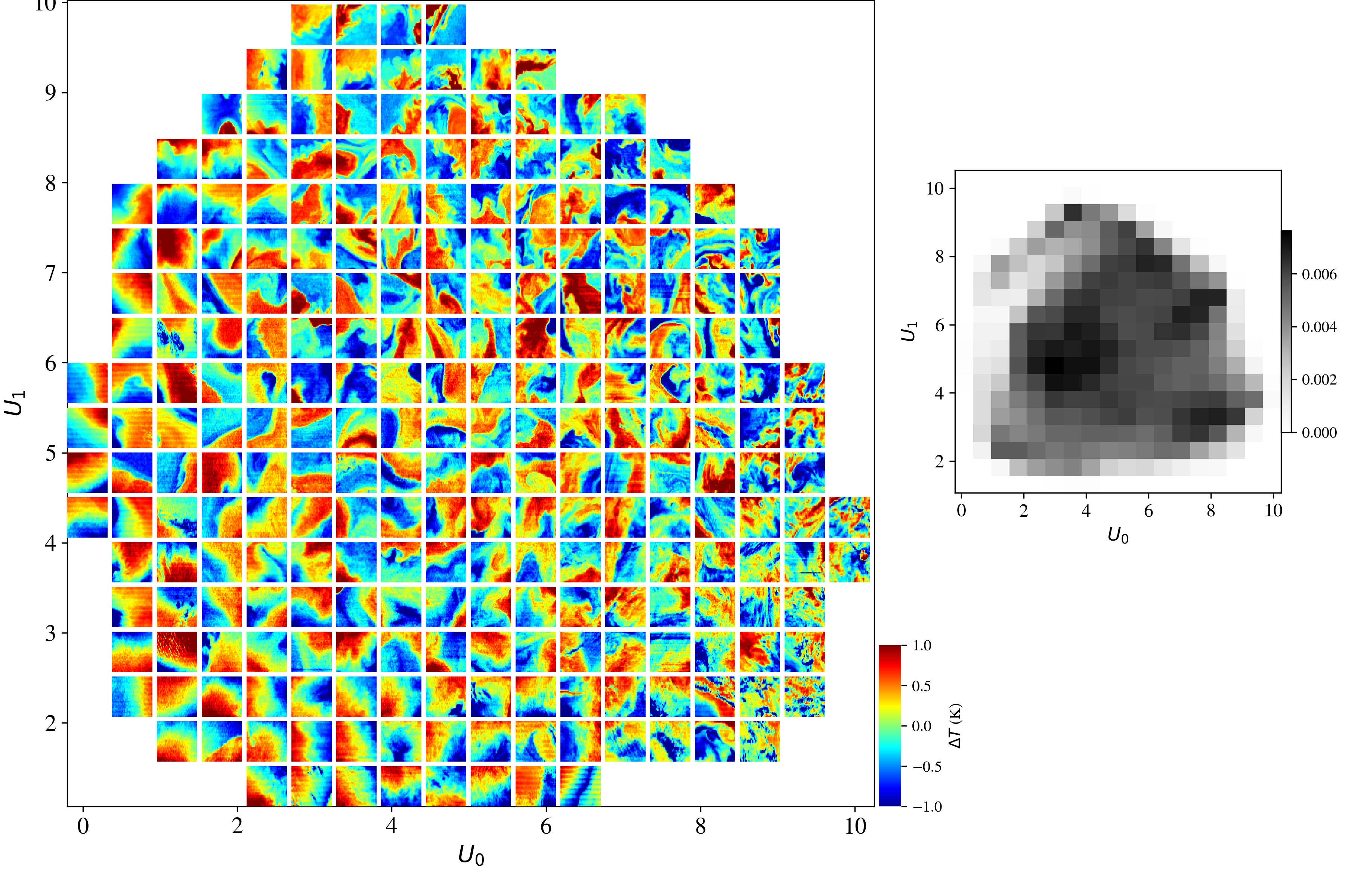
Figure 18: Same as Figure 7 but for the UMAP embedding of the $\Delta T=1-1.5\,{\rm K}$ sub-set of cutouts.

3. ${\Delta T=1-1.5}$ K; 1126838 cutouts; Figure 18

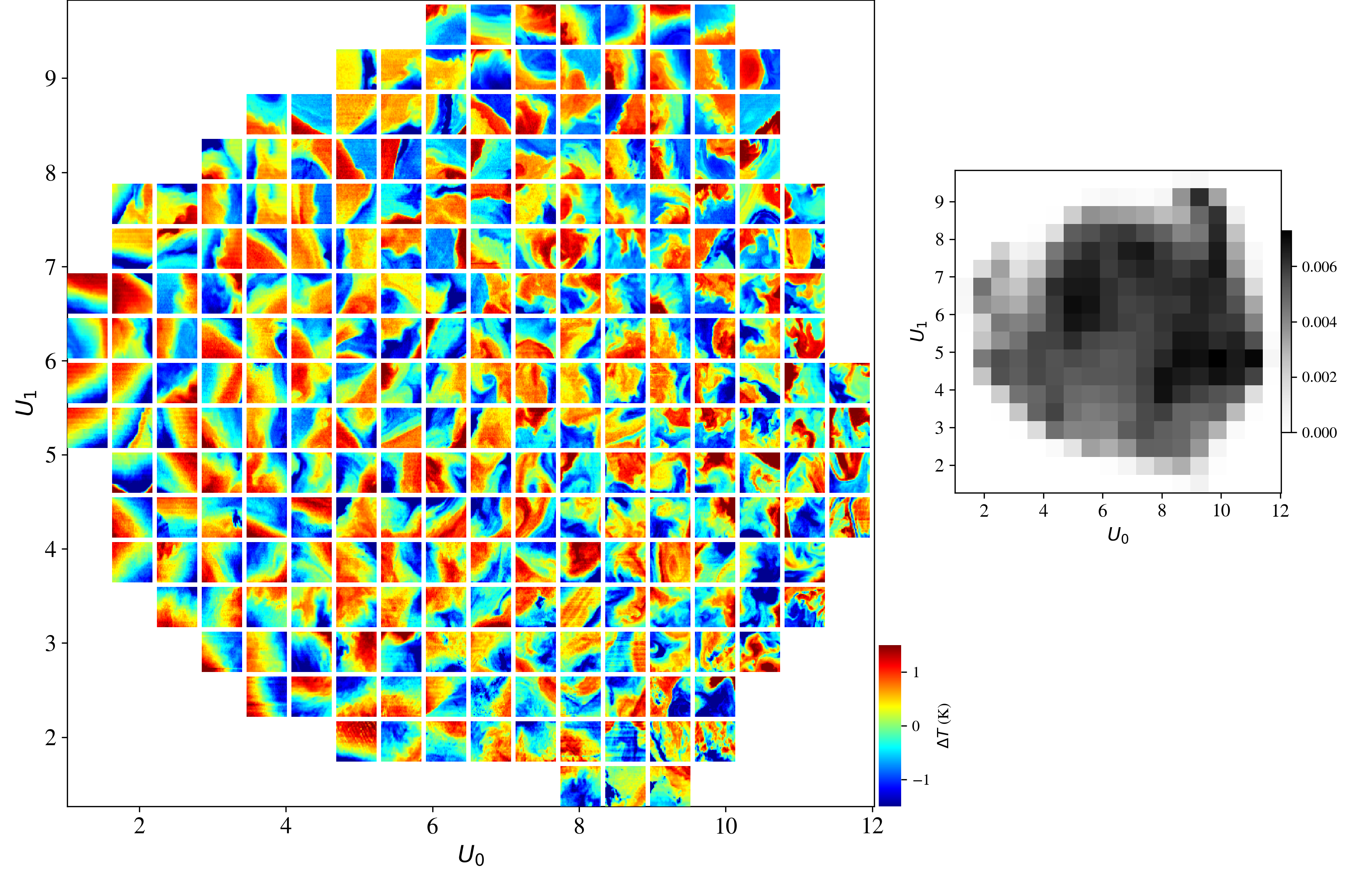
Figure 19: Same as Figure 7 but for the UMAP embedding of the $\Delta T=1.5-2.5\,{\rm K}$ sub-set of cutouts.

4. ${\Delta T=1.5-2.5}$ K; 535038 cutouts; Figure 19

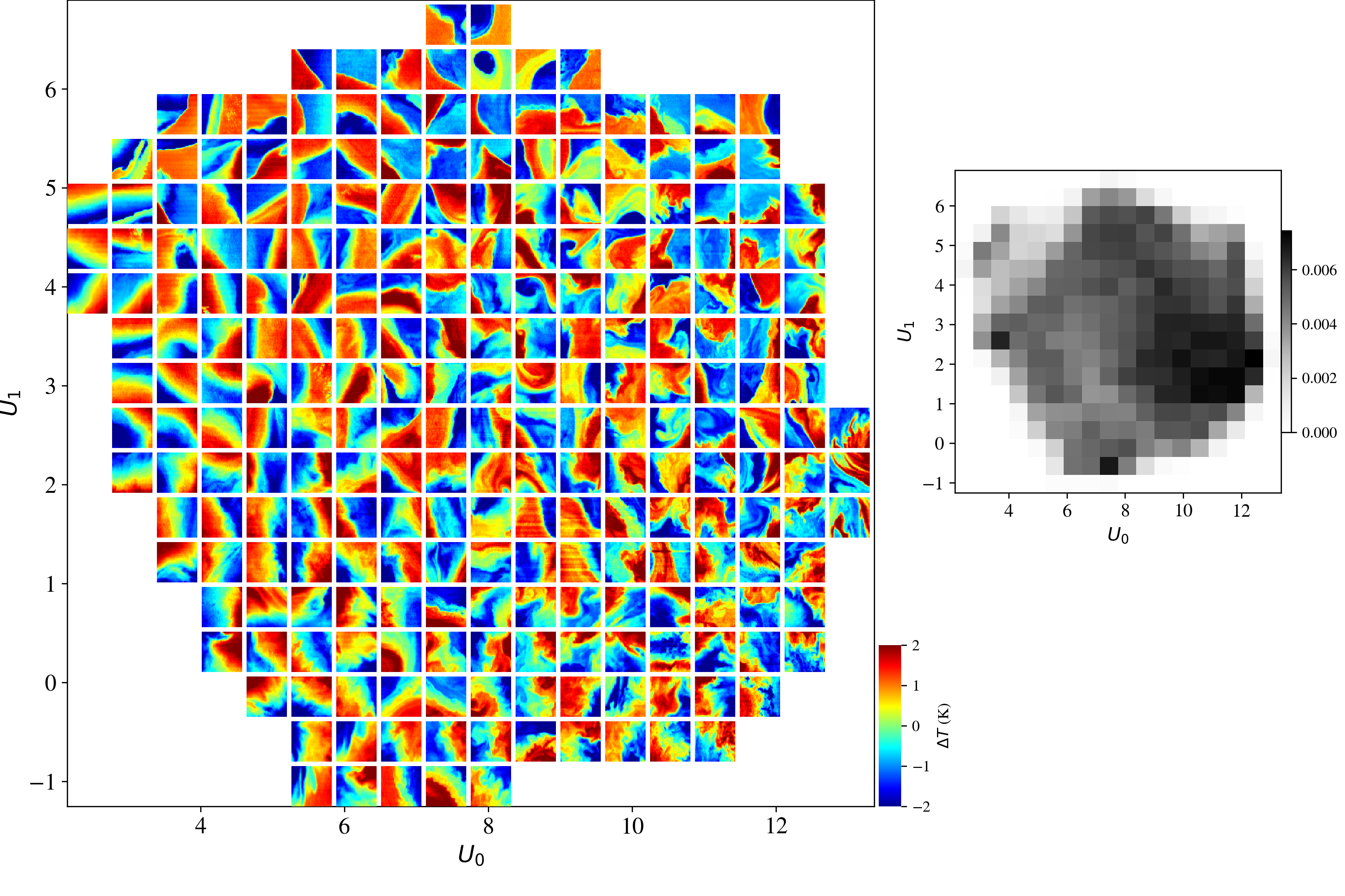
Figure 20: Same as Figure 7 but for the UMAP embedding of the $\Delta T=2.5-4\,{\rm K}$ sub-set of cutouts.

5. ${\Delta T=2.5-4}$ K; 126576 cutouts; Figure 20

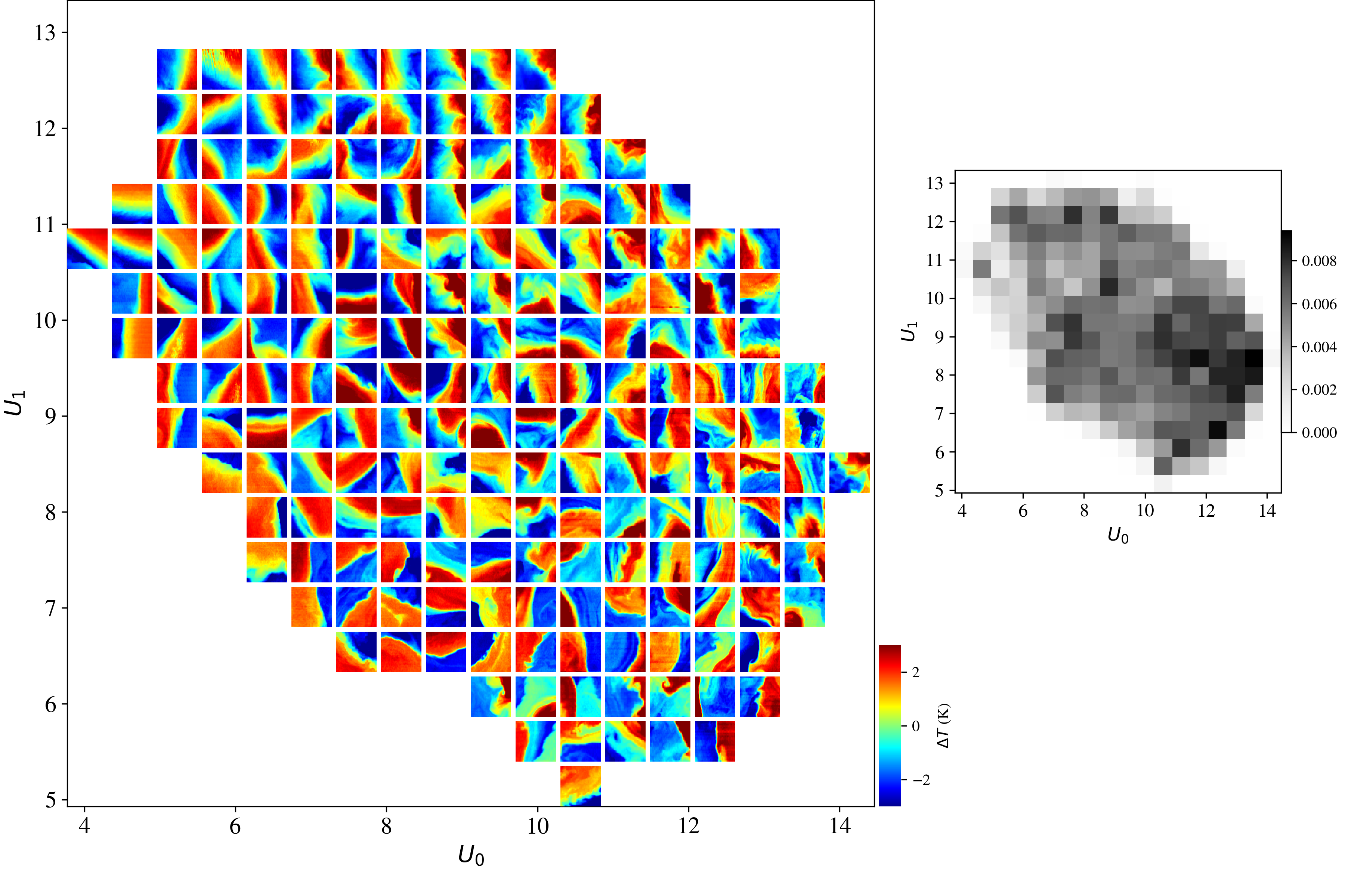
Figure 21: Same as Figure 7 but for the UMAP embedding of the $\Delta T>4\,{\rm K}$ sub-set of cutouts.

6. ${\Delta T>4}$ K; 18317 cutouts; Figure 21

This otherwise arbitrary binning was chosen to minimize $\Delta T$ as a defining factor in the analysis while maintaining large samples of cutouts. Figure 8a shows the UMAP representation of the $\Delta T=0.5-1\,{\rm K}$ sub-sample colored by $\Delta T$. While there is structure in the domain that correlates with $\Delta T$, it is no longer monotonic and cutouts with the full range of $\Delta T$ are located throughout (the standard deviation in $\Delta T$ is $\sigma(\Delta T)\approx 0.13$ K; see Figure 8b).

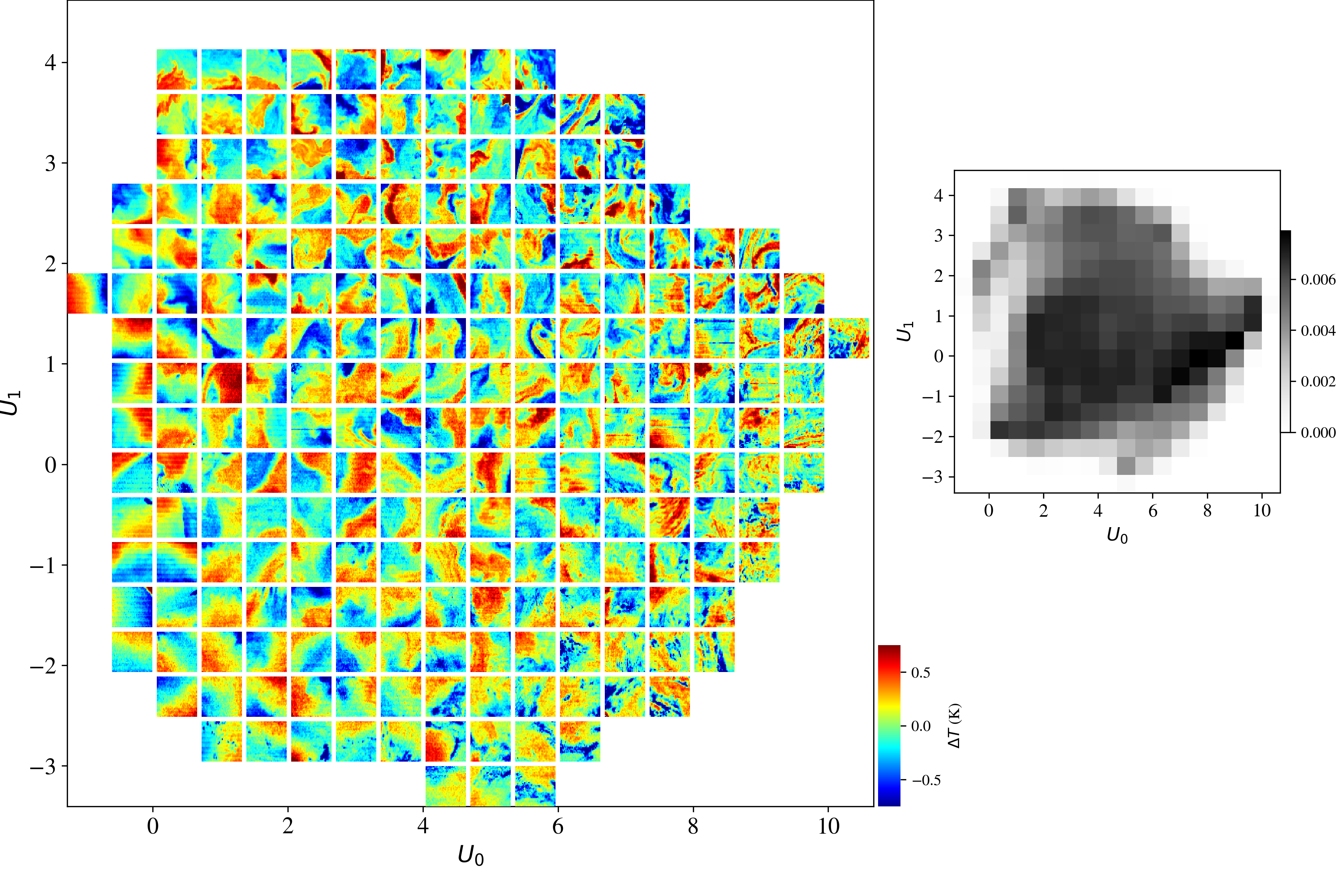
Figure 9: As in Figure 7 but for the UMAP embedding of the $\Delta T=0.5-1\,{\rm K}$ sub-set of cutouts (3,320,395 in total; a cutout is only shown in $U_{0},U_{1}$ bins where there are at least 1,000). In contrast to the full set where the UMAP space was largely defined by the $\Delta T$ of each cutout, this embedding separates the patterns by finer features. Spanning the domain, one identifies a diversity of patterns with structure on the full range of scales. As designed, Nenya has effectively generated a vocabulary to describe and distinguish between the fundamental patterns of SST.

Figure 9 shows a gallery of randomly selected cutouts for the $\Delta T=0.5-1\,{\rm K}$ subset at their binned $U_{0},U_{1}$ values (restricted to areas with at least 1000 cutouts per bin). Examining the figure, one observes a great diversity in the patterns as one travels throughout the UMAP space. One identifies features for which SSTa contours are predominantly linear (e.g., at low $U_{0},U_{1}$), curved (e.g., $U_{0},U_{1}\approx 8,2$) or amorphous (e.g., $U_{0},U_{1}\approx 4,4$), patterns with apparent symmetry about an axis (e.g., $U_{0},U_{1}\approx 0,2$) and those without any discernible structure (e.g., $U_{0},U_{1}\approx 9,1$).

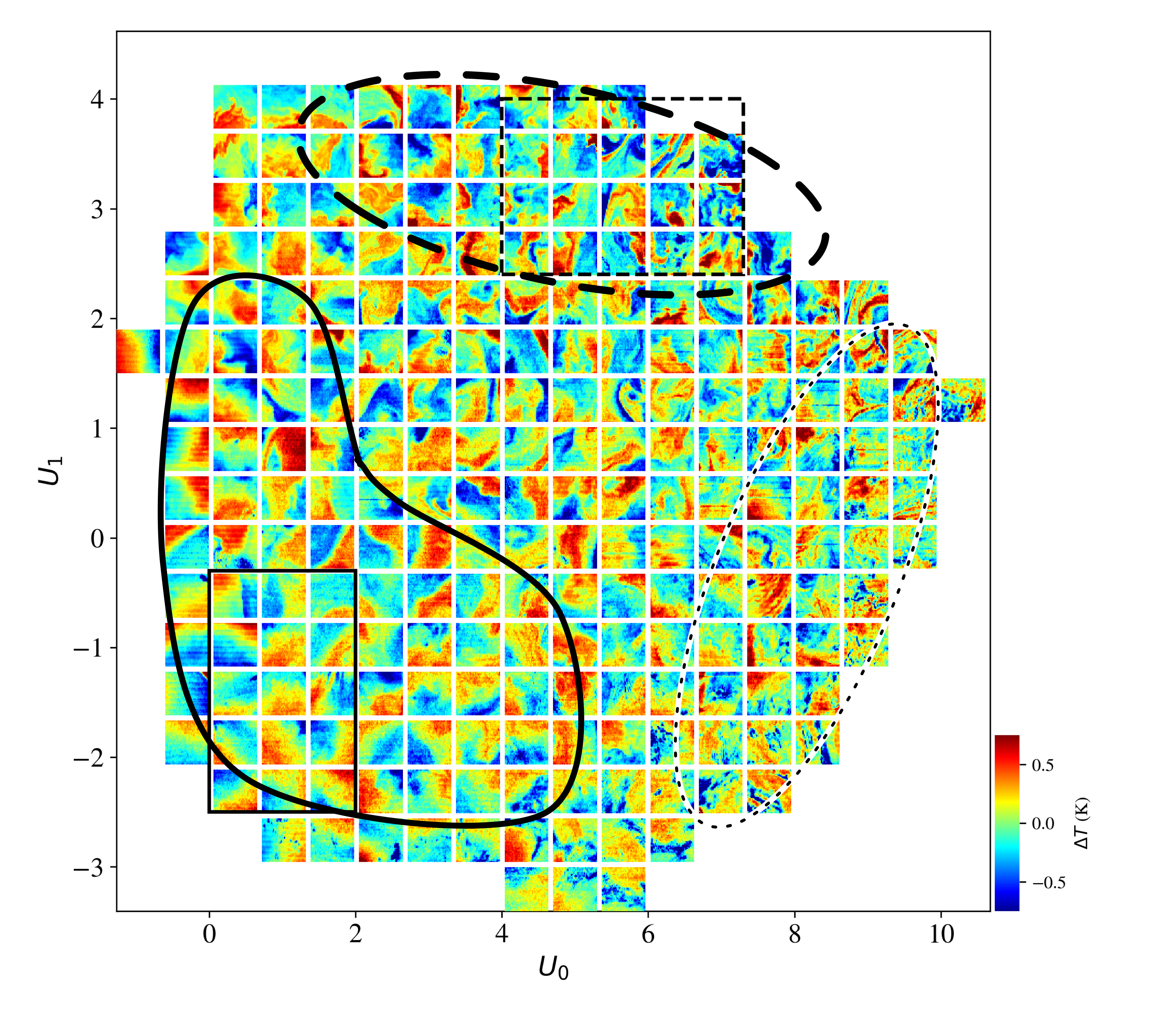
Figure 10: A reproduction of the UMAP domain in Figure 9 but now annotated to highlight regions of interest in the UMAP space. The annotations approximately designate regions where the patterns show: (solid-line annotation) temperature variance predominantly at the largest wavelengths; (dashed-line ellipse) temperature variance reflective of an energetic spectrum, e.g. non-linear, or turbulent motions; and (dash-dot ellipse) patterns with “noisy” features, predominantly on the smallest scales. Meanwhile, the black rectangles (solid and dashed) in the left panel indicate the portions of the UMAP domain analyzed in Figures 11 and 12.

To build additional intuition for the patterns resolved by Nenya, we show a series of properties of the cutouts in Figure 8, binned by $U_{0}$ and $U_{1}$. The characteristic most highly correlated with the pattern distribution in the UMAP embedding is the absolute latitude $|{\rm latitude}|$ (Figure 8e). Given the $|{\rm latitude}|$ dependence for the radius of deformation, this suggests the patterns have been separated by the dominant feature scale, especially along the $U_{1}$ dimension. Visual inspection supports this hypothesis to an extent, e.g. the patterns with largest-scale variance have lower $U_{1}$. On the other hand, cutouts with the smallest scale features arise at high $U_{0}$ and low $U_{1}$ corresponding to mid-latitudes. These also have the highest cloud coverage fraction (Figure 8d) and close inspection of individual cutouts reveals small-scale blemishes characteristic of clouds. We believe these have been missed by the standard screening algorithm and future work may leverage Nenya to flag corrupt data and/or improve the screeing process.

Figure 8c shows the median spectral slope $\alpha_{\rm min}$ which varies across the domain. The values are all negative, indicative of reduced energy at high wavenumbers and, thus, consistent with all theories of geophysical turbulence [14, 15, 16] (cf. section II-C). The pattern dependence on $\alpha_{\rm min}$ is complex with very differing imagery having similar median $\alpha_{\rm min}$. Similarly the standard deviation of $\alpha_{\rm min}$ is large (not shown) Together, these indicate $\alpha_{\rm min}$ is an incomplete descriptor of SST patterns and features.

To better guide analysis presented in the following section, Figure 10 shows the UMAP with several sub-regions annotated to approximately demarcate several types of patterns: those with temperature variance predominantly on the largest scales (solid annotation), cutouts with an “energetic” spectrum showing structure at a range of scales (dashed ellipse), and noisy patterns with structure predominantly on the smallest scales (dash-dot ellipse).

Galleries for the other $\Delta T$ sub-samples are provided in the Appendix (Figures 17-21). Together with Figure 9 these six UMAP spaces span the full diversity of SST patterns, as encoded in the full SSL latent space. With Nenya, we have constructed a vocabulary that encodes the complex language of SST imagery on sub-mesoscales. Any SST cutout drawn from the MODIS L2 dataset maps directly to one of the 6 galleries and is–by design–very similar to its neighboring cutouts in UMAP space. This enables novel exploration of the data–e.g., the ability to define and investigate regions of the ocean with special or unique SST signatures.

Before proceeding, however, a cautionary note is warranted. Because a unique UMAP embedding is generated for the latent vectors in each $\Delta T$ bin, the meaning of the $U_{0}$ and $U_{1}$ axes likely differ from one $\Delta T$ bin to the next. Having said this, we note that with the exception of the gallery for $\Delta T$ $=0-0.5$ K (Fig. 17) all of the galleries show the complexity (e.g., curvature of SSTa contours) increasing as $U_{1}$ increases. That is, setting aside the effect of $\Delta T$, this may be the primary distinguishing characteristic of the fields identified by Nenya.

V Applications and Discussion

In the previous section, we presented the fundamental patterns of SST imagery learned by the Nenya model on scales smaller than $\approx 80$ km. We now demonstrate several applications enabled by constructing this vocabulary to describe the complex patterns of these data. In particular, one may explore the nature and origins of specific patterns across the ocean or the patterns that manifest in select regions, and explore temporal variability. In this section, we focus on the $\Delta T=0.5-1\,{\rm K}$ subset and emphasize that the primary results are largely insensitive to this choice.

V-A Geographical Exploration

A defining characteristic of data collected by remote sensing satellites such as Aqua is their global coverage of the ocean. Using the Nenya model, we may select specific patterns of SST and reveal their global geographic locations. We may then assess commonality (or otherwise) between the processes that generate them. Alternatively, we may select specific local regions to highlight the SST patterns that define them. Here, we consider each of these approaches in turn.

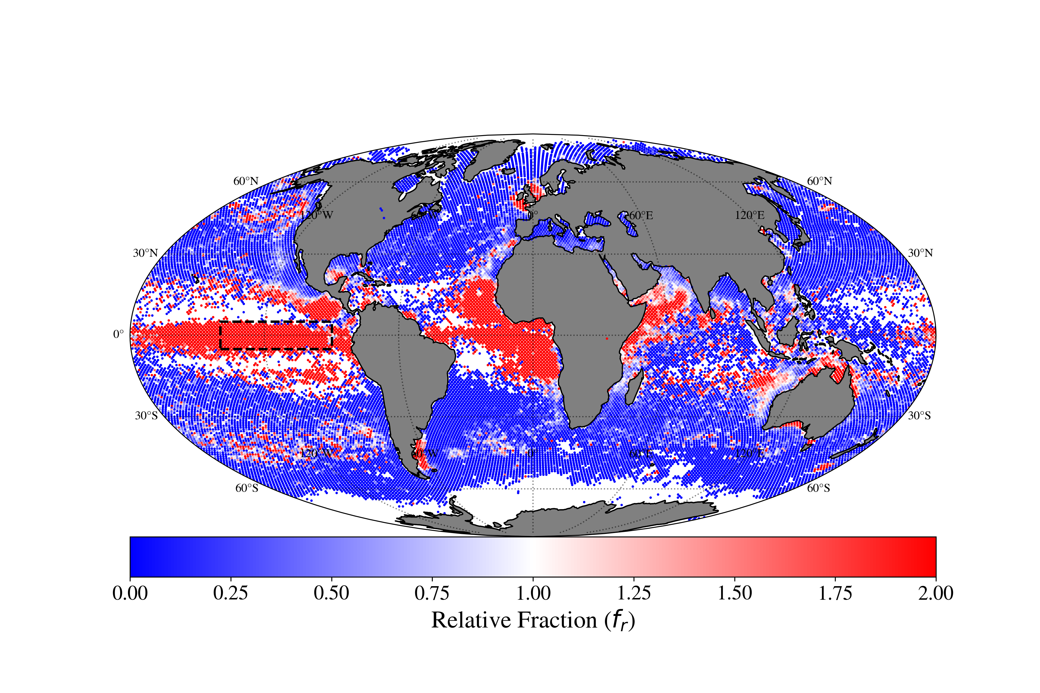
Figure 11: Relative fraction $f_{r}$ of SST cutouts with temperature variance predominantly on large scales ($\approx 80$ km) from the $\Delta T=0.5-1\,{\rm K}$ subset (specified by the dashed rectangle in Figure 9). A low value (blue) implies that the geographic location, with area of $\approx 100\times 100$ km², rarely exhibits such patterns while $f_{r}\geq 1$ (pink/red) indicates an excess. Gray regions indicate land. The figure reveals that large-scale patterns arise primarily at lower latitudes (e.g., the equatorial Pacific and coastal Africa), but also along the Patagonia shelf and Northern Sea. Regions with fewer than 5 cutouts in the $\Delta T$ interval are indicated in white and have not been included in the analysis. The dashed black rectangle is the focus area for Fig. 13.

V-A1 Global

To perform a global analysis, we have divided the surface of the ocean using the Hierarchical Equal Area isoLatitude Pixelation (HEALPix) procedure which tesselates a spherical surface into equal-area curvilinear quadrilaterals [22]. Specifically, we adopted nside=64, which divides the globe into $\approx 50,000$ HEALPix cells each with approximately 100$\times$100 km² area. We then perform statistics on the cutouts which occur within each of these HEALPix cells.

As a first example, we consider cutouts with patterns that exhibit temperature variance predominantly on the largest scales of our augmented images (i.e., $80$ km). Specifically, we select the portion of the UMAP domain corresponding to $\Delta T=0.5-1\,{\rm K}$ with $U_{0}=[0,2]\,{\rm and}\,U_{1}=[-2.5,-0.3]$. This includes $\approx 225,000$ cutouts from the lower left corner of the domain (Figure 10; solid rectangle).

Let us now define a relative fraction $f_{r}$ for each HEALPix which is the ratio of two fractions: (i) $f_{H}$, the fraction of cutouts in the HEALPix which lie within the UMAP rectangle defined above and; (ii) $f_{T}$, the total fraction of all cutouts for the given $\Delta T$ range that lie within the same rectangle. We then calculate

$$f_{r}\equiv\frac{f_{H}}{f_{T}}$$ (3)

for each HEALPix cell, ignoring cells with fewer than 5 cutouts. Small values of $f_{r}$ indicate the pattern (characterized in UMAP-space) occurs rarely within the HEALPix relative to the average, and vice-versa.

Figure 11 presents the geographic distribution of $f_{r}$ for $U_{0}=[0,2]\,{\rm and}\,U_{1}=[-2.5,-0.3]$ in the $\Delta T=0.5-1\,{\rm K}$ bin (Figure 10; solid rectangle). Focusing on geographical regions with an enhanced incidence of these patterns ($f_{r}>1$), we find the majority occur in large, coherent regions ($\gg 100$ km), i.e., much larger than the cutouts analyzed by the Nenya model. In this case, the SST patterns have tagged processes on scales substantially larger than the sub-mesoscale. One also notes that these areas are primarily at low latitudes; this follows physical intuition that the high radius of deformation near the equator leads to larger-scale features. We briefly describe processes that may generate the underlying SST patterns in several of these regions.

Two of the largest regions with high $f_{r}$ in Figure 11 are along the eastern equatorial Pacific and Atlantic. These areas are commonly referred to as the Pacific and Atlantic equatorial cold tongue (ECT), and are of interest to climate studies owing to their impact on air-sea interactions (e.g., [23, 24]). Briefly, ECTs are believed to result from upwelling associated with northward wind stresses in the eastern portion of each basin. This water is then forced by zonal winds to propagate westward [23, 25, 24]. Figure 11 indicates the ECTs exhibit similar SST patterns that span several thousands of kilometers along the equator, stretching to $\approx 180^{\circ}$ W in the Pacific and nearly across the entire Atlantic. The Pacific ECT is confined to a meridional extent of approximately $\pm 5^{\circ}$. In the following section, we examine its seasonal variation.

To the north (at $\approx 10^{\circ}$ N) and distinct from each ECT is an additional region of high relative frequency, one off the coast of Central America and another off the coast of western Africa. Each region is characterized by (seasonal) coastal upwelling and poleward currents [26, 27]. For example, in the Eastern Tropical Pacific, off the coast of Central America, seasonally-varying and intense wind “jets” generate westward-propagating Rossby waves and/or mesoscale eddies in this region [28]. The SST patterns accentuated in this region, however, are not characteristic of such dynamics (see below); we expect the large-scale temperature variance arises from different processes hereto not explored by previous studies. The Atlantic region, meanwhile, corresponds approximately to the “shadow zone” of the eastern tropical North Atlantic and the so-called Guinea dome below it [29, 27]. These have weak circulation and our results suggest, unexpectedly, that the prevailing SST signatures within them are large-scale temperature variations.

Distinct from the enhanced regions at lower latitudes are the waters off the Patagonia shelf. This region is characterized by a shallow continental shelf and the nearby confluence of two strong currents: the equatorward-flowing Malvanis current which meets the poleward-traveling Brazilian current at $\approx 40^{\circ}$S. The circulation on the shelf is predicted (and observed) to be relatively weak [30]. We hypothesize that bathymetry plays a leading role in the generation of the observed SST patterns, which is supported by the orientation of the large-scale temperature variance in the cutouts. We also note that the waters off eastern Africa at $\approx 5^{\circ}$N share features common to the Patagonia shelf [31]; perhaps bathymetry is a driving factor for its high $f_{r}$, as well.

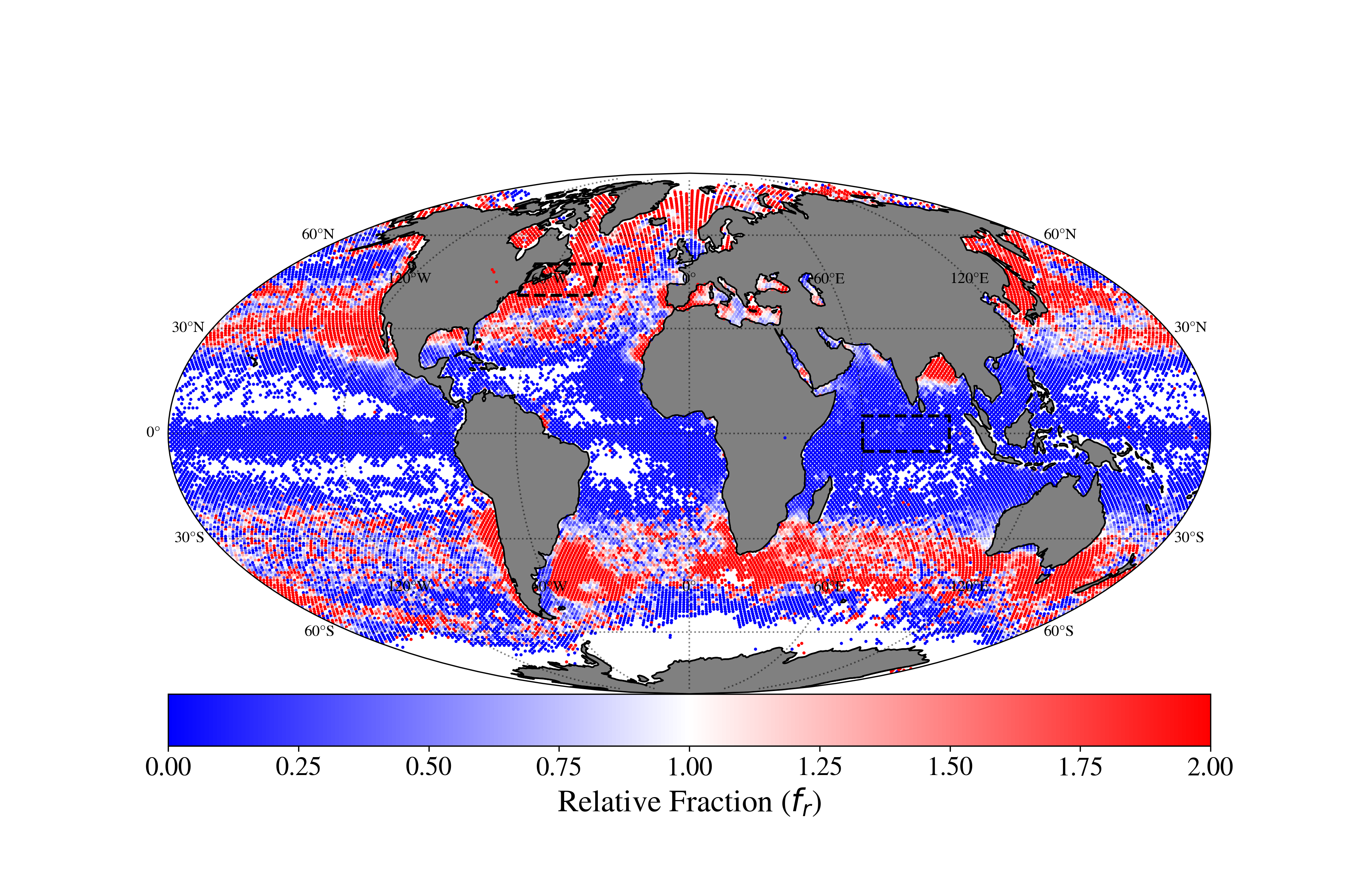
Figure 12: Same as Figure 11 but for SST patterns with structure across a range of scales and from the $\Delta T=0.5-1\,{\rm K}$ subset (specifically $U_{0}=[4,7.3]\,{\rm and}\,U_{1}=[2.4,4]$). The regions that show a high fraction of these turbulent patterns are predominantly those influenced by western boundary currents and areas generally known to show frequent eddy formation and propagation [32]. Strong upwelling may also generate these patterns in select regions: coastal California, western Africa, Chile. We also emphasize the the Bay of Bengal whose dynamics are driven by qualitatively different processes [33]. Dashed black rectangles on the Gulf Stream near New England and the equatorial Indian Ocean are the focus areas for Fig. 14.

In an effort to contrast the geographical distribution of the large-scale SST patterns of Figure 11 with that for cutouts suggesting a significantly shorter range of scales, we now focus on SST patterns for which $\Delta T=0.5-1\,{\rm K}$ with $U_{0}=[4,7.3]\,{\rm and}\,U_{1}=[2.4,4]$ (Figure 10; dashed rectangle). Their complex patterns are suggestive of regions in which non-linear, sub-mesoscale dynamics (e.g., eddies and filaments) and/or ageostrophic turbulence are to be found.

Figure 12 presents the relative frequency $f_{r}$ of these patterns. All of the geographical regions in Figure 11 with high relative fractions now have low $f_{r}$, and an entirely distinct set of locations with high $f_{r}$ appear. These are primarily poleward of $20^{\circ}$ deg and may be divided into four main groups. (1) waters associated with strong open-ocean currents (e.g., the Brazil-Malvanis confluence, the Gulf Stream, the Kuroshio, the Agulhas Retroflection); (2) enclosed or semi-enclosed seas (e.g., parts of the Mediterranean, the Sea of Japan, the Okhotsk Sea, the southern end of the Red Sea, the northern half of the Gulf of Mexico, the Baltic Sea); (3) eastern boundaries of most ocean basins in the subtropics (e.g., off California and Mexico, Chile, Northwest Africa); and (4) anomalous regions equatorward of $22.5^{\circ}$: the Bay of Bengal and the retroflection of a portion of the South Equatorial Current into the Equatorial Countercurrent off of northern Brazil and French Guiana.

As noted above the first group is associated with strong currents and comprise regions where eddies frequently form (e.g., [32]). Several are also noted regions of strong upwelling, e.g., coastal California [34]. Neither of these are a surprise. By contrast, a significant fraction of virtually all major enclosed or semi-enclosed seas comprise cutouts for which SST contours show signs of relatively small spatial scales while these regions show little to no signs of long wavelength contours (Fig. 11). Is this because topography is complex in these regions exerting significant control over circulation? Or, maybe land constrains the flow both of currents and winds resulting in smaller scale motion? Regardless, the implications here are intriguing.

We may speculate–given the randomly-selected cutouts presented in UMAP-space–that the SST patterns with $f_{r}>>1$ Figure 12 trace regions of active frontogensis, frontoloysis, and frontal instabilities at scales defined as sub-mesoscale ($\lambda<50\,\rm km$) and therefore enhanced ageostrophic turbulence. It is an active area of interest for the authors to connect such processes to the specific SST patterns defined by Nenya.

Last, a visual inspection of the cutouts with high $U_{0}$ and low $U_{1}$ in the dotted ellipse of Figure 10 shows signatures of clouds, e.g., patterns of speckled, cooler patches. These are primarily cases that passed through the cloud-screening algorithms [35] of the R2019.0 MODIS processing. In this respect, our Nenya model has efficiently identified corrupt fields. We have examined the geographic distribution of these cutouts and found they generally track the overall distribution of data, although there is a preference for mid-latitudes.

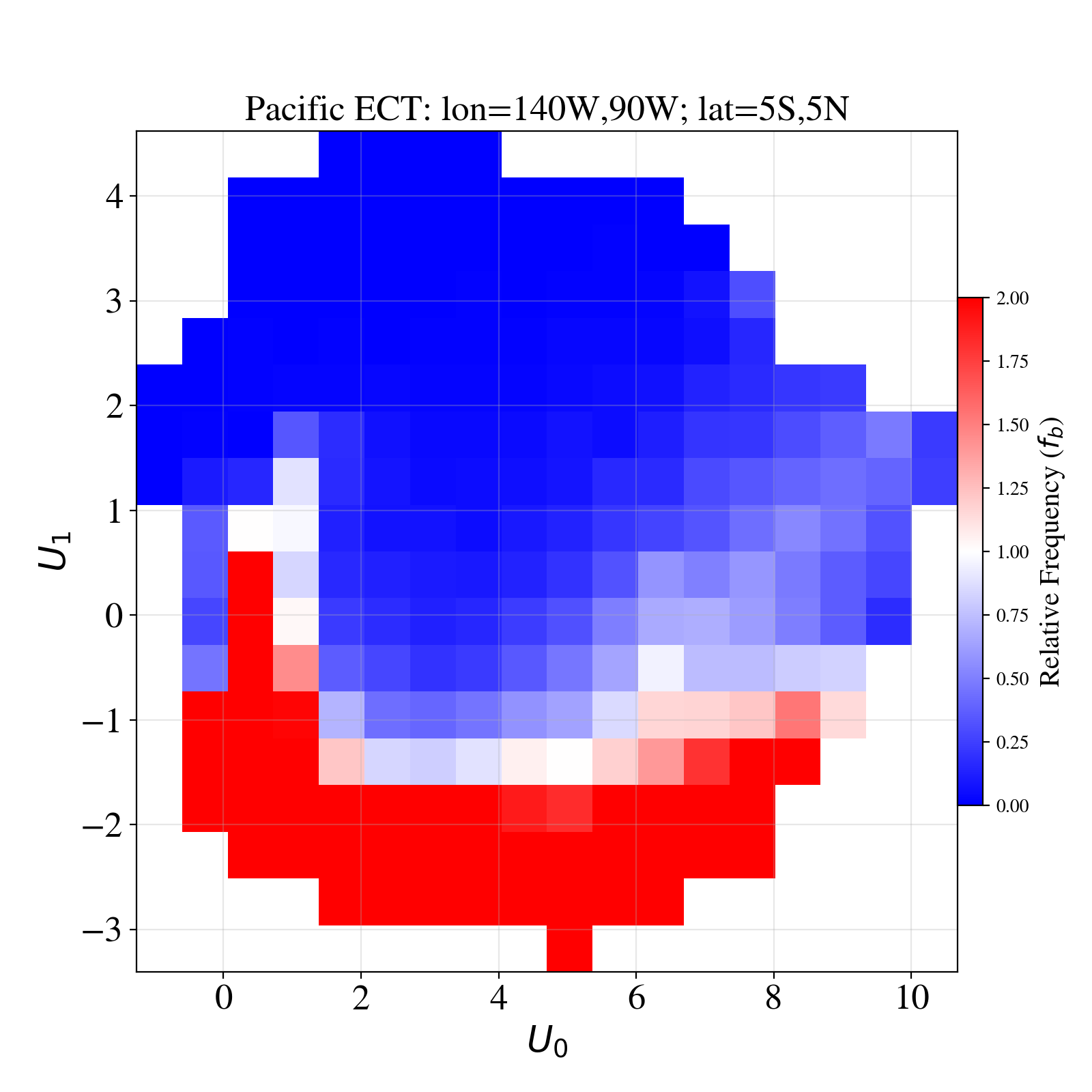
Figure 13: Two-dimensional histogram of the relative frequency of specific SST patterns for $\Delta T=0.5-1\,{\rm K}$ in the Pacific ECT This region is identified by the dashed black rectangle in Fig. 11 and contains 81,675 cutouts. The Pacific region is dominated by patterns with temperature variance at large scales (low $U_{1}$ and low $U_{0}$) and patterns with blemishes suggestive of unmasked clouds (low $U_{1}$ and high $U_{0}$). Bins with fewer than 200 cutouts have been excluded from the panels.

V-A2 Local

We may effectively invert the above analysis to examine the SST patterns that are dominant in select geographical regions. As an example, Figure 13 shows the relative frequency, corresponding to the $\Delta T=0.5-1\,{\rm K}$ subset, of SST patterns in the Pacific ECT (black dashed rectangle in Figure 11). For this analysis, we have divided the UMAP domain into $18\times 18$ equal-spaced bins that span 99.9% of each dimension ($\Delta U_{0}\approx 0.65$ and $\Delta U_{1}\approx 0.45$). We then calculate a relative frequency of occurrence $f_{b}$, defined as the frequency of cutouts for the region in each bin $f_{R}$ divided by the frequency measured for the entire ocean $f_{O}$:

$$f_{b}\equiv\frac{f_{R}}{f_{O}}\;\;.$$ (4)

High $f_{b}$ values therefore indicate SST patterns that are more characteristic of the region than that of the global ocean. These $f_{b}$ maps are the SST “fingerprints” of the regions specifying the SST patterns they preferentially manifest.

Examining Figure 13, we find the Pacific ECT shows an excess of SST patterns with low $U_{1}$; these are a combination of cutouts with large-scale structure and cutouts with significant “blemishes”, which we identify as unmasked clouds. The patterns with $f_{b}<1$ for the Pacific ECT, meanwhile, are those with temperature variance across a range of scales including small scales. We conclude it is very rare for such fluctuations to occur in this region, i.e., the westward propagation of the ECT is stable against such instabilities. Additional exploration reveals that features likely associated with tropical instability waves that occur along the meridional periphery of the ECT [36] have larger scale gradients and higher $\Delta T$ (e.g., at $U_{0},U_{1}\approx 6,8$ in Figure 19).

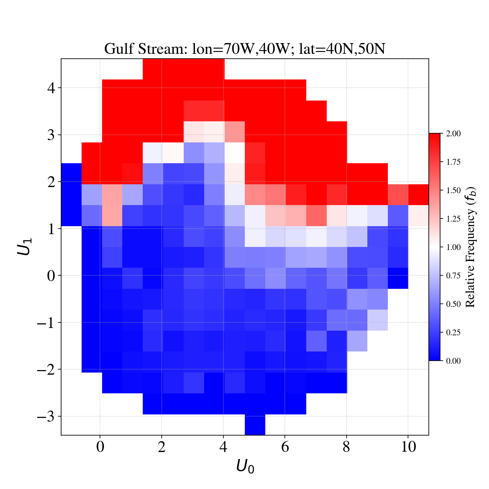
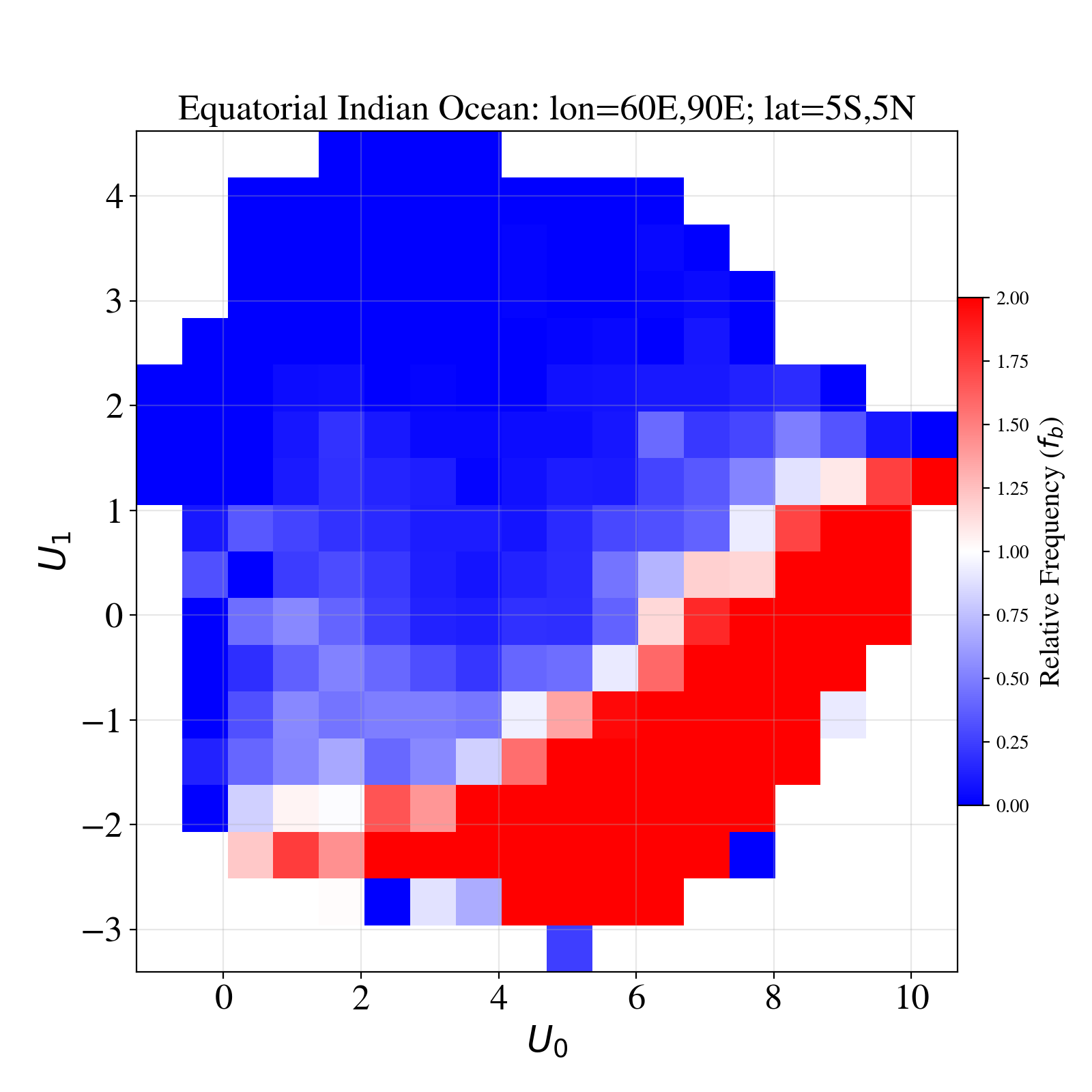
Figure 14: Similar to Figure 13 but for SST patterns of the $\Delta T=0.5-1\,{\rm K}$ subset and for the Gulf Stream near New England (top) and the Equatorial Indian Ocean (bottom). The precise regions evaluated are labeled on the figures and shown in Figure 12 and each contains approximately 10,000 cutouts. The Gulf Stream shows an excess of patterns within the energetic region of the UMAP space (dashed ellipse in Figure 10) which have temperature variance at a wide range of scales. In contrast, the Equatorial Indian Ocean primarily exhibits patterns with small-scale variations, including those most similar to white noise (described by the dotted ellipse in Figure 10).

Two more local regions are presented in Figure 14. These highlight two areas from Figure 12: one with a high relative fraction (the Gulf Stream near New England) indicative of a highly dynamic region, and one with low $f_{r}$ (the equatorial Indian Ocean). The dominant SST patterns of the Gulf Stream are drawn from the high $U_{1}$ portion of the UMAP domain (Figure 14), especially the energetic region annotated in Figure 10 (dashed ellipse). These patterns show the highest degree of complexity with temperature variance at a range of scales, and features with strong curvature, and strong gradients. By the same token, the Gulf Stream avoids the regions of the UMAP domain where cutouts show predominantly large-scale or small-scale structures (solid and dotted annotations respectively in Figure 10). Together, the $f_{b}$ distribution in the upper panel of Figure 14 identifies the SST patterns that manifest in highly dynamic regions (e.g., near and within western boundary currents).

The lower panel of Figure 14 describes the SST patterns prevalent in the equatorial Indian Ocean. These occur predominantly within the lower-right portion of the UMAP domain (dotted annotation in Figure 10). This region contains primarily cutouts with isolated, cooler patches (e.g., unmasked clouds) and those dominated by small-scale variance. Likewise, it is very rare for this portion of the Indian Ocean to exhibit temperature variations on medium to larger scales.

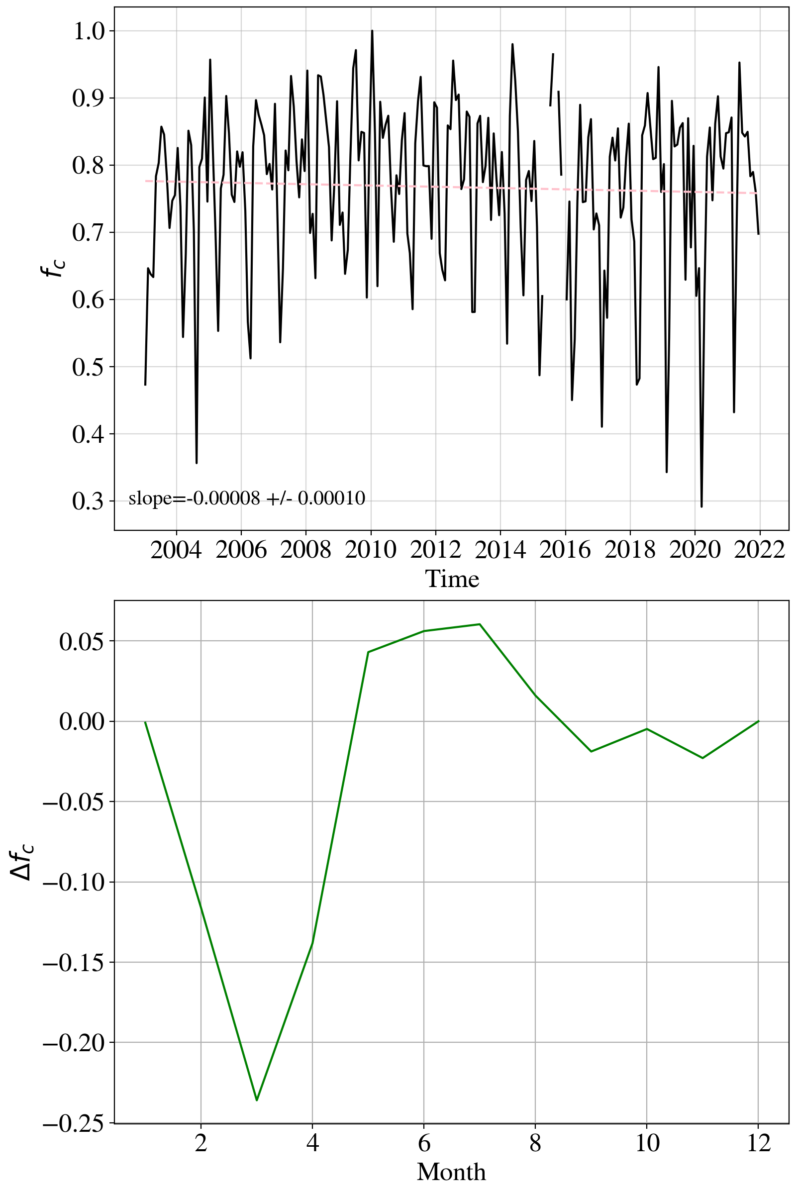
Figure 15: Time series analysis of the cutout fraction for the prominent SST patterns of the Pacific ECT (limited to $\Delta T=0.5-1\,{\rm K}$). These are defined by the portion of the UMAP domain where $f_{b}>1.5$ in Figure 13. A cutout fraction $f_{c}$=1 indicates all of the cutouts in that month and year have these patterns. The upper panel shows the full time-series of $f_{c}$ and the dashed line is a fit to the inter-annual trend accounting for seasonal variations. There is a strong seasonal signature (lower panel) associated with the intensification of the ECT by an increase in northward wind stress [23].

V-B Temporal Change

In addition to the extenstive (global) geographic coverage afforded by remote sensing observations, the MODIS dataset now spans nearly two decades of daily observations. This permits a time-series analysis of the incidence of SST patterns characteristic of particular dynamics. We consider both long-term (i.e., inter-annual) and short-term (seasonal) trends in select regions.

Returning to the Pacific ECT, we perform a time-series analysis for its prominent SST patterns. We define these patterns as the portion of the UMAP domain for the $\Delta T=0.5-1\,{\rm K}$ sample that have a relative frequency $f_{b}>1.5$, i.e., the red regions in Figure 13. For each month of each year in the dataset, we calculate the fraction of cutouts $f_{c}$ in that portion of the UMAP domain. If there are fewer than 10 cutouts in a given month and year, that time-stamp is ignored.

The time-series of $f_{c}$ and its seasonal and inter-annual analysis is plotted in Figure 15. The time-series analysis models the data assuming a linear trend for any inter-annual variation and 11 free parameters for the months January-November to assess seasonal variations (the results are relative to December). A strong seasonal component is apparent with the boreal summer months (May-September) dominant and with the ECT suppressed from February-March inclusive. The enhancement has been associated with the intensification of the Pacific ECT by air-sea interactions [37, 38]. There is no significant linear inter-annual trend, but we do observe that the near-disappearance of the ECT (low $f_{c}$) in February/March has been intensifying over the past $\sim 10$ years.

Turning to a portion of Gulf Stream near New England, we isolate the cutouts with $f_{b}>1.25$ in the upper panel of Figure 14 which are those with complex patterns. Similar to the Pacific ECT, the primary SST patterns of the Gulf Stream exhibit a strong seasonal dependence (Figure 16). Its seasonal trend, however, is (coincidentally) out-of-phase with the ECT showing the highest $f_{c}$ in winter months and a great deficit in mid-summer. The latter may occur as a significant seasonal thermocline is formed in the area to the north and west of the Gulf Stream effectively obscuring the more turbulent waters beneath.

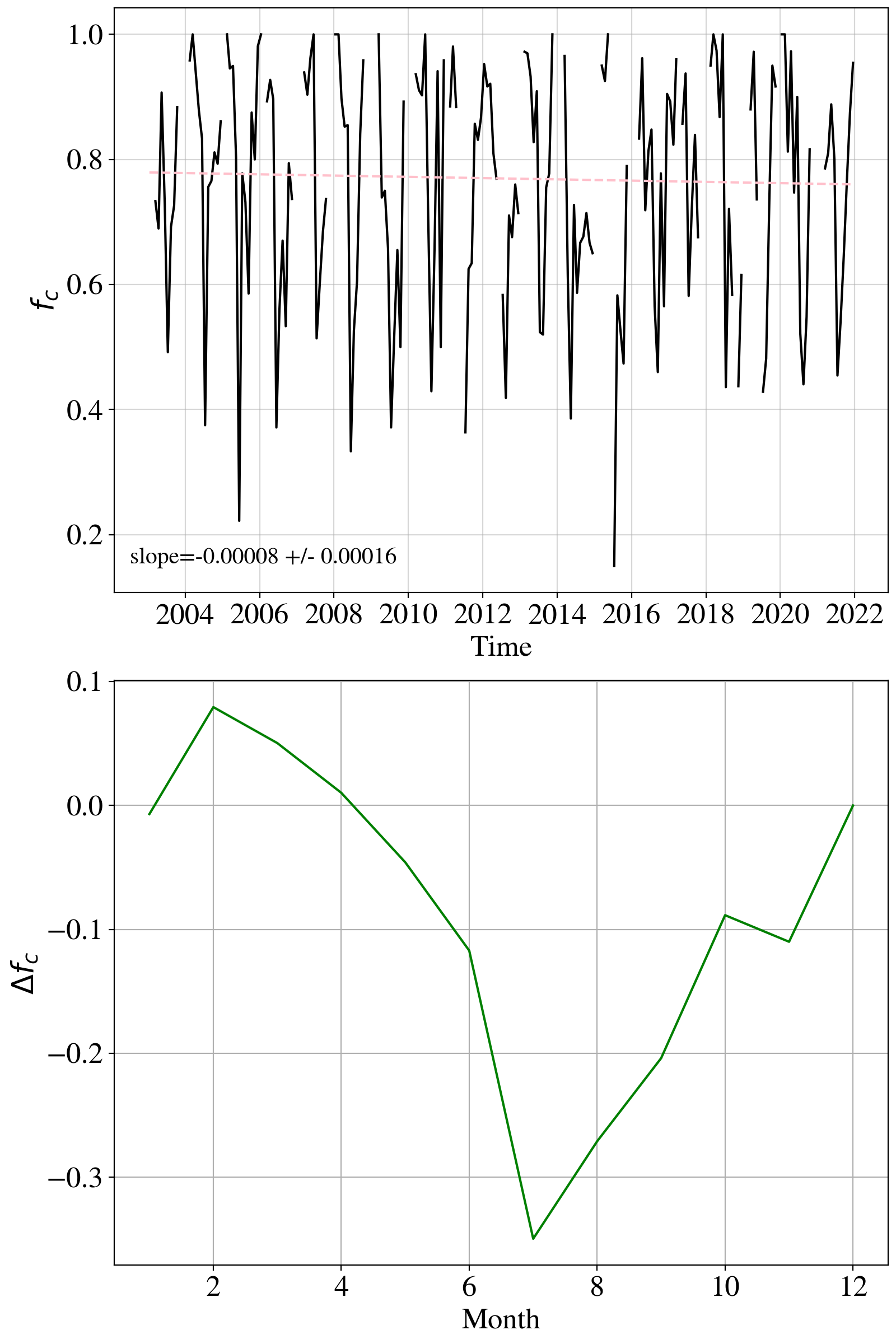
Figure 16: Same as for Figure 15 but for the enhanced patterns of the Gulf Stream near New England, those with $f_{b}>1.25$ in the upper panel of Figure 14. The incidence of these complex patterns exhibits a strong seasonal dependence, with a strong suppression during summer months possibly due to masking by the seasonal thermocline.

VI Summary and Concluding Remarks

We have designed a deep, contrastive learning model to reveal and resolve the fundamental patterns of SST for the global ocean on scales of $\approx 80\times 80\,\rm km^{2}$ (i.e., sub-mesoscale). This Nenya model is intentionally invariant to vertical and horizontal flips, rotations, and small translations. We trained Nenya on 600,000 random cutouts from the MODIS L2 night-time dataset in the years 2003-2021 inclusive. To readily explore the 256-dimension latent space that defines the complexity of SST patterns, we bin the cutouts by $\Delta T$–the size of its 90% SST interval–and generated a UMAP transformation of the latent vectors to 2-dimensions.

We confirmed that Nenya has successfully separated the SST patterns in this 3-dimensional space (one for $\Delta T$, and 2 for each UMAP) to describe the full complexity of SST imagery. We identify SST patterns with structures on scales ranging from the $\approx 2$ km sampling of the data to the full extent of the cutouts. Furthermore, Nenya separates patterns with predominantly linear structures from those with significant curvature. In essence, Nenya defines a vocabulary for the language of SST imagery at the sub-mesoscale.

Leveraging this vocabulary, we examined the preferred geographical distribution of several sets of SST patterns. Nenya reveals that SST patches with temperature variance on scales larger than the sub-mesoscale occur preferentially in several distinct and large regions at low latitudes. These include the Pacific and Atlantic ECTs where the westward propagation of cool waters upwelled from eastern areas in the basin yield large temperature gradients along the equator. Additionally, we find that complex SST patterns with significant temperature variance on scales ranging from a few to tens of kilometers arise predominantly in dynamically active regions (e.g., western boundary currents) at high latitudes. These results confirm the direct mapping from SST patterns to distinct ocean processes.

Another application of Nenya is to resolve the principal SST patterns in select geographical regions. We recover highly distinct distributions of SST patterns when comparing the Pacific ECT (temperature variations primarly on large scales), a portion of the Gulf Stream near New England (complex SST patterns with temperature variance at a range of scales), and the Equatorial Indian Ocean (primarily small-scale temperature variations). The distributions of these SST patterns are a fingerprint that define the regions and the dominant near-surface processes in these regions.

Last, we performed a time-series analysis of the defining patterns of the Pacific ECT and the Gulf Stream near New England to search for inter-annual and seasonal trends. We identify seasonal trends for each: the strengthening of the ECT in mid-summer months and the depression of dynamic features in/near the Gulf Stream during the summer.

We conclude, at least statistically, that a vocabulary that defines SST patterns provides a novel approach to tracking physical processes across the global ocean and dissecting such processes within distinct regions. Emboldened by this success, we will regress these patterns, specifically the full latent space representation of Nenya, against specific dynamic processes (e.g., frontogenesis) to leverage SST as an indirect descriptor of such dynamics. This will require performing analysis and training on ocean model output with known dynamics, e.g., the LLC4320 ocean general circulation model [39, 40, 41]. Ultimately, we may track the roles of sub-mesoscale processes in mixing and energy dissipation across the globe over the past two decades.

With this publication, we provide all of the data, outputs, and software related to Nenya and this manuscript. We also provide on-line visualization tools that enable the community to explore SST patterns from the dataset and those provided by the user. See XXX for full details.

TABLE I: MODIS Cutouts

lon	lat	date	$\Delta T$	$\alpha_{\rm min}$	LL	$U_{0,\rm all}$	$U_{1,\rm all}$	$U_{0}$	$U_{1}$
(deg)	(deg)		(K)
8.688	-32.425	2003-01-01 00:35:00	0.495	-1.86	172.7	3.9	3.5	-1.6	5.3
9.434	-33.705	2003-01-01 00:35:00	0.655	-1.77	204.6	0.1	2.7	6.8	2.2
10.311	-33.231	2003-01-01 00:35:00	0.689	-1.83	90.3	1.8	2.0	9.1	1.6
8.381	-33.559	2003-01-01 00:35:00	0.712	-2.18	188.9	-0.3	3.6	7.4	0.9
9.303	-32.807	2003-01-01 00:35:00	0.754	-1.85	137.0	2.0	1.2	9.0	1.2
9.151	-33.372	2003-01-01 00:35:00	0.536	-1.68	212.0	-0.7	2.6	8.0	0.9
11.091	-33.327	2003-01-01 00:35:00	0.470	-1.87	274.6	2.7	2.2	-0.0	0.8
10.385	-32.951	2003-01-01 00:35:00	0.605	-1.77	149.0	2.4	2.0	8.9	0.2
11.023	-33.612	2003-01-01 00:35:00	0.374	-1.93	312.6	3.3	3.6	-0.4	1.1
9.030	-32.474	2003-01-01 00:35:00	0.645	-1.78	183.6	1.0	2.1	8.1	1.6
9.940	-33.183	2003-01-01 00:35:00	0.679	-1.95	110.6	1.5	3.3	9.2	1.5
9.176	-31.906	2003-01-01 00:35:00	0.415	-2.05	242.9	2.3	3.1	0.3	4.3
9.506	-33.420	2003-01-01 00:35:00	0.707	-1.63	187.1	0.3	2.8	8.3	1.0
9.869	-33.468	2003-01-01 00:35:00	0.715	-2.07	108.1	0.8	1.9	8.9	1.9
8.613	-32.710	2003-01-01 00:35:00	0.518	-1.83	161.0	3.7	3.7	9.4	0.8
8.348	-32.376	2003-01-01 00:35:00	0.418	-1.86	162.4	4.4	3.9	-2.0	5.3
10.016	-32.903	2003-01-01 00:35:00	0.565	-1.82	152.3	2.6	3.7	8.9	0.6
10.241	-33.515	2003-01-01 00:35:00	0.748	-2.05	111.9	1.2	1.7	9.0	1.9
10.454	-32.666	2003-01-01 00:35:00	0.412	-1.67	249.4	3.8	3.1	-0.6	4.6
11.876	-33.711	2003-01-01 00:35:00	0.386	-1.95	384.9	3.9	4.6	1.6	4.0
10.085	-32.618	2003-01-01 00:35:00	0.420	-1.69	250.1	3.8	3.5	-0.4	4.4

Notes: The $\Delta T$ value listed here is measured from the inner $40\times 40$ pixel² region of the cutout.
LL is the log-likelihood metric calculated from the Ulmo algorithm.
$U_{0,\rm all},U_{1,\rm all}$ are the UMAP values for the UMAP analysis on the full dataset.
$U_{0},U_{1}$ are the UMAP values for the UMAP analysis in the $\Delta T$ bin for this cutout.

Acronyms

(A)ATSR

one or all of ATSR, ATSR-2 and AATSR

AATSR

Advanced Along Track Scanning Radiometer

ACC

Antarctic Circumpolar Current

ACCESS

Advancing Collaborative Connections for Earth System Science

ACL

Access Control List

ACSPO

Advanced Clear Sky Processor for Oceans

ADA

Automatic Detection Algorithm

ADCP

Acoustic Doppler Current Profiler

ADT

absolute dynamic topography

AESOP

Assessing the Effects of Submesoscale Ocean Parameterizations

AGU

American Geophysical Union

AI

Artificial Intelligence

AIRS

Atmospheric Infrared Sounder

AIS

Ancillary Information Service

AIST

Advanced Information Systems Techonology

AISR

Applied Information Systems Research

ADL

Alexandria Digital Library

API

Application Program Interface

APL

Applied Physics Laboratory

API

Application Program Interface

AMSR

Advanced Microwave Scanning Radiometer

AMSR2

Advanced Microwave Scanning Radiometer 2

AMSR-E

Advanced Microwave Scanning Radiometer - EOS

ANN

Artificial Neural Network

AOOS

Alaska Ocean Observing System

APAC

Australian Partnership for Advanced Computing

APDRC

Asia-Pacific Data-Research Center

ARC

ATSR Reprocessing for Climate

ASCII

American Standard Code for Information Interchange

AS

Aggregation Server

ASFA

Aquatic Sciences and Fisheries Abstracts

ASTER

Advanced Spaceborne Thermal Emission and Reflection Radiometer

ATBD

Algorithm Theoretical Basis Document

ATSR

Along Track Scanning Radiometer

ATSR-2

Second ATSR

AVISO

Archiving, Validation and Interpretation of Satellite Oceanographic Data

ANU

Australian National University

AVHRR

Advanced Very High Resolution Radiometer

AzC

Azores Current

BAA

Broad Agency Announcement

BAO

bi-annual oscillation

BES

Back-End Server

BMRC

Bureau of Meteorology Research Centre

BOM

Bureau of Meteorology

BT

brightness temperature

BUFR

Binary Universal Format Representation

CAN

Cooperative Agreement Notice

CAS

Community Authorization Service

CC

cloud cover

CCA

Cayula-Cornillon Algoritm

CCI

Climate Change Initiative

CCLRC

Council for the Central Laboratory of the Research Councils

CCMA

Center for Coastal Monitoring and Assessment

CCR

cold core ring

CCS

California Current System

CCSM

Community Climate System Model

CCSR

Center for Climate System Research

CCV

Center for Computation and Visualization

CDAT

Climate Data Analysis Tools

CDC

Climate Diagnostics Center

CDF

Common Data Format

CDR

Common Data Representation

CEDAR

Coupled Energetic and Dynamics and Atmospheric Regions

CEOS

Committee on Earth Observation Satellites

CERT

Computer Emergency Response Team

CenCOOS

Central & Northern California Ocean Observing System

CF

clear fraction

CGI

Common Gateway Interface

CHAP

CISL High Performance Computing Advisory Panel

CIFS

Common Internet File System

CIMSS

Cooperative Institute for Meteorological Satellite Studies

CIRES

Cooperative Institute for Research (in) Environmental Sciences

CISL

Computational & Information Systems Laboratory

CLASS

Comprehensive Large Array-data Stewardship System

CLIVAR

Climate Variability and Predictability

CLS

Collecte Localisation Satellites

CME

Community Modeling Effort

CMS

Centre de Météorologie Spatiale

CNN

Convolutional Neural Network

COA

Climate Observations and Analysis

COARDS

Cooperative Ocean-Atmosphere Research Data Standard

COAPS

Center for Ocean-Atmospheric Prediction Studies

COBIT

Control Objectives for Information and related Technology

COCO

CCSR Ocean Component model

CODAR

Coastal Ocean Dynamics Applications Radar

CODMAC

Committee on Data Management, Archiving, and Computing

Co-I

Co-Investigator

CORBA

Common Object Request Broker Architecture

COLA

Center for Ocean-Land-Atmosphere Studies

CPU

Central Processor Unit

CRS

Coordinate Reference System

CSA

Cambridge Scientific Abstracts

CSC

Coastal Services Center

CSIS

Center for Strategic and International Studies

CSL

Constraint Specification Language

CSP

Chermayeff, Sollogub and Poole, Inc.

CSDGM

Content Standard for Digital Geospatial Metadata

CSV

Comma Separated Values

CTD

Conductivity, Temperature and Salinity

CVSS

Common Vulnerability Scoring System

CZCS

Coastal Zone Color Scanner

DAAC

Distribute Active Archive Center

DAARWG

Data Archiving and Access Requirements Working Group

DAP

Data Access Protocol

DAS

Data set Attribute Structure

DBMS

Data Base Management System

DBDB2

Digital Bathymetric Data Base

DChart

Dapper Data Viewer

DDS

Data Descriptor Structure

DDX

XML version of the combined DAS and DDS

DFT

Discrete Fourier Transform

DIF

Directory Interchange Format

DISC

Data and Information Services Center

DIMES

Diapycnal and Isopycnal Mixing Experiment: Southern Ocean

DMAC

Data Management and Communications committee

DMR

Department of Marine Resources

DMSP

Defense Meteorological Satellite Program

DoD

Department of Defense

DODS

Distributed Oceanographic Data System

DOE

Department of Energy

DSP

U. Miami satellite data processing software

DSS

direct statistical simulation

EASy

Environmental Analysis System

ECCO

Estimating the Circulation and Climate of the Ocean

ECCO2

Estimating the Circulation and Climate of the Ocean Phase II

ECS

EOSDIS Core System

ECT

equatorial cold tongue

ECHO

Earth Observing System Clearinghouse

ECMWF

European Centre for Medium-range Weather Forecasting

ECV

Essential Climate Variable

EDC

Environmental Data Connector

EDJ

Equatorial Deep Jet

EDFT

Extended Discrete Fourier Transform

EDMI

Earth Data Multi-media Instrument

EEJ

Extra-Equatorial Jet

EIC

Equatorial Intermediate Current

EICS

Equatorial Intermediate Current System

EJ

Equatorial Jets

EKE

eddy kinetic energy

EMD

Empirical Mode Decomposition

EOF

Empirical Orthogonal Function

EOS

Earth Observing System

EOSDIS

Earth Observing System Data Information System

EPA

Environmental Protection Agency

EPSCoR

Experimental Program to Stimulate Competitive Research

EPR

East Pacific Rise

ERD

Environmental Research Division

ERS

European Remote-sensing Satellite

ESA

European Space Agency

ESDS

Earth Science Data Systems

ESDSWG

Earth Science Data Systems Workign Group

ESE

Earth Science Enterprise

ESG

Earth System Grid

ESG II

Earth System Grid – II

ESIP

Earth Science Information Partner

ESMF

Earth System Modeling Framework

ESML

Earth System Markup Language

ESP

eastern South Pacfic

ESRI

Environmental Systems Research Institute

ESR

Earth and Space Research

ETOPO

Earth Topography

EUC

Equatorial Undercurrent

EUMETSAT

European Organisation for the Exploitation of Meteorological Satellites

Ferret

FASINEX

Frontal Air-Sea Interaction Experiment

FDS

Ferret Data Server

FFT

Fast Fourier Transform

FGDC

Federal Geographic Data Committee

FITS

Flexible Image (or Interchange) Transport System

FLOPS

FLoating point Operations Per Second

FRTG

Flow Rate Task Group

FreeForm

FNMOC

Fleet Numerical Meteorology and Oceanography Center

FSU

Florida State University

FTE

Full Time Equivalent

ftp

File Transport Protocol

ftp

File Transport Protocol

GAC

Global Area Coverage

GAN

Generative Adversarial Network

GB

GigaByte - $10^{9}$ bytes

GCMD

Global Change Master Directory

GCM

general circulation model

GCOM-W1

Global Change Observing Mission - Water

GCOS

Global Climate Observing System

GDAC

Global Data Assembly Center

GDS

GrADS Data Server

GDS2

GHRSST Data Processing Specification v2.0

GEBCO

General Bathymetric Charts of the Oceans

GeoTIFF

Georeferenced Tag Image File Format

GEO-IDE

Global Earth Observation Integrated Data Environment

GES DIS

Goddard Earth Sciences Data and Information Services Center

GEMPACK

General Equilibrium Modelling PACKage

GEOSS

Global Earth Observing System of Systems

GFDL

Geophysical Fluid Dynamics Laboratory

GFD

Geophysical Fluid Dynamics

GHRSST

Group for High Resolution Sea Surface Temperature

GHRSST-PP

GODAE High Resolution Sea Surface Temperature Pilot Project

GINI

GOES Ingest and NOAA/PORT Interface

GIS

Geographic Information Systems

Globus

GMAO

Global Modeling and Assimilation Office

GML

Geography Markup Language

GMT

Generic Mapping Tool

GODAE

Global Ocean Data Assimilation Experiment

GOES

Geostationary Operational Environmental Satellites

GOFS

Global Ocean Forecasting System

GoMOOS

Gulf of Maine Ocean Observing System

GOOS

Global Ocean Observing System

GOSUD

Global Ocean Surface Underway Data

GPFS

General Parallel File System

GPU

Graphics Processing Unit

GRACE

Gravity Recovery and Climate Experiment

GRIB

GRid In Binary

GrADS

Grid Analysis and Display System

GridFTP

FTP with GRID enhancements

GRIB

GRid in Binary

GPS

Global Positioning System

GSFC

Goddard Space Flight Center

GSI

Grid Security Infrastructure

GSO

Graduate School of Oceanography

GTSPP

Global Temperature and Salinity Profile Program

GUI

Graphical User Interface

GS

Gulf Stream

HAO

High Altitude Observatory

HLCC

Hawaiian Lee Countercurrent

HCMM

Heat Capacity Mapping Mission

HDF

Hierarchical Data Format

HDF-EOS

Hierarchical Data Format - EOS

HEALPix

Hierarchical Equal Area isoLatitude Pixelation

HEC

High-End Computing

HF

High Frequency

HGE

High Gradient Event

HPC

High Performance Computing

HPCMP

High Performance Computing Modernization Program

HPSS

High Performance Storage System

HR DDS

High Resolution Diagnostic Data Set

HRPT

High Resolution Picture Transmission

HTML

Hyper Text Markup Language

html

Hyper Text Markup Language

http

the hypertext transport protocol

HTTP

Hyper Text Transfer Protocol

HTTPS

Secure Hyper Text Transfer Protocol

HYCOM

HYbrid Coordinate Ocean Model

I-band

imagery resolution band

IDD

Internet Data Distribution

IB

Image Band

IBL

internal boundary layer

IBM

Internation Business Machines

ICCs

Intermediate Countercurrents

IDE

Integrated Development Environment

IDL

Interactive Display Language

IDLastro

IDL Astronomy User’s Library

IDV

Integrated Data Viewer

IEA

Integrated Ecosystem Assessment

IEEE

Institute (of) Electrical (and) Electronic Engineers

IETF

Internet Engineering Task Force

IFREMER

Institut Français de Recherche pour l’Exploitation de la MER

IMAPRE

El Instituto del Mar del Perú

IMF

Intrinsic Mode Function

IOOS

Integrated Ocean Observing System

ISAR

Infrared Sea surface temperature Autonomous Radiometer

ISO

International Organization for Standardization

ISSTST

Interim Sea Surface Temperature Science Team

IT

Information Technology

ITCZ

Intertropical Convergence Zone

IP

Internet Provider

IPCC

Intergovernmental Panel on Climate Change

IPRC

International Pacific Research Center

IR

infrared

IRI

International Research Institute for Climate and Society

ISO

International Standards Organization

JASON

JASON Foundation for Education

JDBC

Java Database Connectivity

JFR

Juan Fernández Ridge

JGOFS

Joint Global Ocean Flux Experiment

JHU

Johns Hopkins University

JPL

Jet Propulsion Laboratory

JPSS

Joint Polar Satellite System

KDE

Kernel Density Estimation

KVL

Keyword-Value List

KML

Keyhole Markup Language

KPP

K-Profile Parameterization

LAC

Local Area Coverage

LAN

Local Area Network

LAS

Live Access Server

LASCO

Large Angle and Spectrometric Coronagraph Experiment

LatMIX

Scalable Lateral Mixing and Coherent Turbulence

LDAP

Lightweight Directory Access Protocol

LDEO

Lamont Doherty Earth Observatory

LEAD

Linked Environments for Atmospheric Discovery

LEIC

Lower Equatorial Intermediate Current

LES

Large Eddy Simulation

L1

Level-1

L2

Level-2

L3

Level-3

L4

Level-4

LL

log-likelihood

LLC

Latitude/Longitude/polar-Cap

LLC-4320

Latitude/Longitude/polar-Cap (LLC)-4320

LLC-2160

LLC-2160

LLC-1080

LLC-1080

LHF

Latent Heat Flux

LST

local sun time

LTER

Long Term Ecological Research Network

LTSRF

Long Term Stewardship and Reanalysis Facility

LUT

Look Up Table

M-band

moderate resolution band

MABL

marine atmospheric boundary layer

MADT

Maps of Absolute Dynamic Topography

MapServer

MapServer

MAT

Metadata Acquisition Toolkit

MATLAB

MARCOOS

Mid-Atlantic Coastal Ocean Observing System

MARCOORA

Mid-Atlantic Coastal Ocean Observing Regional Association

MB

MegaByte - $10^{6}$ bytes

MCC

Maximum Cross-Correlation

MCR

MATLAB Component Runtime

MCSST

Multi-Channel Sea Surface Temperature

MDT

mean dynamic topography

MDB

Match-up Data Base

MDOT

mean dynamic ocean topography

MEaSUREs

Making Earth System data records for Use in Research Environments

MERRA

Modern Era Retrospective-Analysis for Research and Applications

MERSEA

Marine Environment and Security for the European Area

MTF

Modulation Transfer Function

MICOM

Miami Isopycnal Coordinate Ocean Model

MIRAS

Microwave Imaging Radiometer with Aperture Synthesis

MITgcm

MIT General Circulation Model

MIT

Massachusetts Institute of Technology

mks

meters, kilograms, seconds

MLP

Multilayer Perceptron

ML

machine learning

MLSO

Mauna Loa Solar Observatory

MM5

Mesoscale Model

MMI

Marine Metadata Initiative

MMS

Minerals Management Service

MODAS

Modular Ocean Data Assimilation System

MODIS

MODerate-resolution Imaging Spectroradiometer

MOU

Memorandum of Understanding

MPARWG

Metrics Planning and Reporting Working Group

MSE

mean square error

MSG

Meteosat Second Generation

MTPE

Mission To Planet Earth

MUR

Multi-sensor Ultra-high Resolution

MV

Motor Vessel

NAML

National Association of Marine Laboratories

NAHDO

National Association of Health Data Organizations

NAS

Network Attached Storage

NASA

National Aeronautics and Space Administration

NCAR

National Center for Atmospheric Research

NCEI

National Centers for Environmental Information

NCEP

National Centers for Environmental Prediction

NCDC

National Climatic Data Center

NCDDC

National Coastal Data Development Center

NCL

NCAR Command Language

ncBrowse

NcML

netCDF Markup Language

NCO

netCDF Operator

NCODA

Navy Coupled Ocean Data Assimilation

NCSA

National Center for Supercomputing Applications

NDBC

National Data Buoy Center

NDVI

Normalized Difference Vegetation Index

NEC

North Equatorial Current

NECC

North Equatorial Countercurrent

NEFSC

Northeast Fisheries Science Center

NEIC

North Equatorial Intermediate Current

netCDF

NETwork Common Data Format

NEUC

North Equatorial Undercurrent

NGDC

National Geophysical Data Center

NICC

North Intermediate Countercurrent

NIST

National Institute of Standards and Technology

NLSST

Non-Linear Sea Surface Temperature

NMFS

National Marine Fisheries Service

NMS

New Media Studio

NN

Neural Network

NOAA

National Oceanic and Atmospheric Administration

NODC

National Oceanographic Data Center

NOGAPS

Navy Operational Global Atmospheric Prediction System

NOMADS

NOAA Operational Model Archive Distribution System

NOPP

National Oceanographic Parternership Program

NOS

National Ocean Service

NPP

National Polar-orbiting Partnership

NPOESS

National Polar-orbiting Operational Environmental Satellite System

NSCAT

NASA SCATterometer

NSEN

NASA Science and Engineering Network

NSF

National Science Foundation

NSIPP

NASA Seasonal-to-Interannual Prediction Project

NRA

NASA Research Announcement

NRC

National Research Council

NRL

Naval Research Laboratory

NSCC

North Subsurface Countercurrent

NSF

National Science Foundation

NSIDC

National Snow and Ice Data Center

NSPIRES

NASA Solicitation and Proposal Integrated Review and Evaluation System

NSSDC

National Space Science Data Center

NVODS

National Virtual Ocean Data System

NWP

Numerical Weather Prediction

NWS

National Weather Service

OBPG

Ocean Biology Processing Group

OB.DAAC

Ocean Biology DAAC

ODC

OPeNDAP Data Connector

OC

ocean color

OCAPI

OPeNDAP C API

ODSIP

Open Data Services Invocation Protocol

OFES

Ocean Model for the Earth Simulator

OCCA

OCean Comprehensive Atlas

OGC

Open Geospatial Consortium

OGCM

ocean general circulation model

OISSTv1

Optimally Interpolated SST Version 1

ONR

Office of Naval Research

OLCI

Ocean Land Colour Instrument

OLFS

OPeNDAP Lightweight Front-end Server

OOD

out-of-distribution

OOPC

Ocean Observation Panel for Climate

OPeNDAP

Open source Project for a Network Data Access Protocol

OPeNDAPg

GRID-enabled OPeNDAP tools

OpenGIS

OpenGIS

OSI SAF

Ocean and Sea Ice Satellite Application Facility

OSS

Office of Space Science

OSTM

Ocean Surface Topography Mission

OSU

Oregon State University

OS X

OWL

Web Ontology Language

OWASP

Open Web Application Security Project

PAE

probabilistic autoencoder

PBL

planetary boundary layer

PCA

Principal Components Analysis

PDF

probability distribution function

PDF

probability density function

PF

Polar Front

PFEL

Pacific Fisheries Environmental Laboratory

PI

Principal Investigator

PIV

Particle Image Velocimetry

PL

Project Leader

PM

Project Member

PMEL

Pacific Marine Environmental Laboratory

POC

particulate organic carbon

PO-DAAC

Physical Oceanography – Distributed Active Archive Center

POP

Parallel Ocean Program

PSD

Power Spectral Density

PSPT

Precision Solar Photometric Telescope

PSU

Pennsylvania State University

PyDAP

Python Data Access Protocol

PV

potential vorticity

QC

quality control

QG

quasi-geostrophic

QuikSCAT

Quick Scatterometer

QZJ

quasi-zonal jet

R2HA2

Rescue & Reprocessing of Historical AVHRR Archives

RAFOS

SOFAR, SOund Fixing And Ranging, spelled backward

RAID

Redundant Array of Independent Disks

RAL

Rutherford Appleton Laboratory

RDF

Resource Description Language

REASoN

Research, Education and Applications Solutions Network

REAP

Realtime Environment for Analytical Processing

ReLU

Rectified Linear Unit

REU

Research Experiences for Undergraduates

RFA

Research Focus Area

RFI

Radio Frequency Interference

RFC

Request For Comments

R/GTS

Regional/Global Task Sharing

RSI

Research Systems Inc.

RISE

Radiative Inputs from Sun to Earth

rms

root mean square

RMI

Remote Method Invocation

ROMS

Regional Ocean Modeling System

ROSES

Research Opportunities in Space and Earth Sciences

RSMAS

Rosenstiel School of Marine and Atmospheric Science

RSS

Remote Sensing Sytems

RTM

radiative transfer model

SACCF

Southern ACC Front

(SAC)-D

Satélite de Aplicaciones Científicas-D

SAF

Subantarctic Front

SAIC

Science Applications International Corporation

SANS

SysAdmin, Audit, Networking, and Security

SAR

synthetic aperature radar

SATMOS

Service d’Archivage et de Traitement Météorologique des Observations Spatiales

SBE

Sea-Bird Electronics

SciDAC

Scientific Discovery through Advanced Computing

SCC

Subsurface Countercurrent

SCCWRP

Southern California Coastal Water Research Project

SDAC

Solar Physics Data Analysis Center

SDS

Scientific Data Set

SDSC

San Diego Supercomputer Center

SeaDAS

SeaWiFS Data Analysis System

SeaWiFS

Sea-viewing Wide Field-of-view Sensor

SEC

South Equatorial Current

SECC

South Equatorial Countercurrent

SECDDS

Sun Earth Connection Distributed Data Services

SEEDS

Strategic Evolution of ESE Data Systems

SEIC

South Equatorial Intermediate Current

SEUC

Southern Equatorial Undercurrent

SEVIRI

Spinning Enhanced Visible and Infra-Red Imager

SeRQL

SeRQL

SGI

Silican Graphics Incorporated

SHF

Sensible Heat Flux

SICC

South Intermediate Countercurrent

SIED

single image edge detection

SIPS

Science Investigator–led Processing System

SIR

Scatterometer Image Reconstruction

SISTeR

Scanning Infrared Sea Surface Temperature Radiometer

SLA

sea level anomaly

SMAP

Soil Moisture Active Passive

SMMR

Scanning Multichannel Microwave Radiometer

SMOS

Soil Moisture and Ocean Salinity

SMTP

Simple Mail Transfer Protocol

SOAP

Simple Object Access Protocol

SOEST

School of Ocean and Earth Science and Technology

SOFAR

SOund Fixing And Ranging

SOFINE

Southern Ocean Finescale Mixing Experiment

SOHO

Solar and Heliospheric Observatory

SPARC

Space Physics and Aeronomy Research Collaboratory

SPARQL

Simple Protocol and RDF Query Language

SPASE

Space Physics Archive Search Engine

SPCZ

South Pacific Convergence Zone

SPDF

Space Physics Data Facility

SPDML

Space Physics Data Markup Language

SPG

Standards Process Group

SQL

Structured Query Language

SSCC

South Subsurface Countercurrent

SSL

self-supervised learning

SSO

Single sign-on

SSES

Single Sensor Error Statistics

SSH

sea surface height

SSHA

sea surface height anomaly

SSMI

Special Sensor Microwave/Imager

SST

sea surface temperature

SSTa

SST anomaly

SSS

sea surface salinity

SSTST

Sea Surface Temperature Science Team

STEM

science, technology, engineering and mathematics

STL

Standard Template Library

STCZ

Subtropical Convergence Zone

Suomi-NPP

Suomi-National Polar-orbiting Partnership

SWEET

Semantic Web for Earth and Environmental Terminology

SWFSC

Southwest Fisheries Science Center

SWOT

Surface Water and Ocean Topography

SWRL

Semantic Web Rule Language

SubEx

Submesoscale Experiment

SURA

Southeastern Universities Research Association

SURFO

Summer Undergraduate Research Fellowship Program in Oceanography

SuperDARN

Super Dual Auroral Radar Network

TAMU

Texas A&M University

TB

TeraByte - $10^{12}$ bytes

TCASCV

Technology Center for Advanced Scientific Computing and Visualization

TCP

Transmission Control Protocol

TCP/IP

Transmission Control Protocol/Internet Protocol

TDS

THREDDS Data Server

TEX

external temperature or T-External

THREDDS

Thematic Realtime Environmental Data Distributed Services

TIDI

TIMED Doppler Interferometer

TIFF

Tag Image File Format

TIMED

Thermosphere, Ionosphere, Mesosphere, Energetics and Dynamics

TLS

Transport Layer Security

TRL

Technology Readiness Level

TMI

TRMM Microwave Imager

TOPEX/Poseidon

TOPography EXperiment for Ocean Circulation/Poseidon

TRMM

Tropical Rainfall Measuring Mission

TSG

thermosalinograph

UCAR

University Corporation for Atmospheric Research

UCSB

University of California, Santa Barbara

UCSD

University of California, San Diego

uCTD

Underway Conductivity, Temperature and Salinity or Underway CTD

UDDI

Universal Description, Discovery and Integration

UMAP

Uniform Manifold Approximation and Projection

UMiami

University of Miami

Unidata

URI

University of Rhode Island

UPC

Unidata Program Committee

URL

Uniform Resource Locator

USGS

United States Geological Survey

UTC

Coordinated Universal Time

UW

University of Washington

VCDAT

Visual Climate Data Analysis Tools

VIIRS

Visible-Infrared Imager-Radiometer Suite

VR

Virtual Reality

VSTO

Virtual Solar-Terrestrial Observatory

WCR

Warm Core Ring

WCS

Web Coverage Service

WCRP

World Climate Research Program

WFS

Web Feature Service

WMS

Web Map Service

W3C

World Wide Web Consortium

WJ

Wyrtki Jets

WHOI

Woods Hole Oceanographic Institution

WKB

Well Known Binaries

WIMP

Windows, Icons, Menus, and Pointers

WIS

World Meteorological Organisation Information System

WOA05

World Ocean Atlas 2005

WOCE

World Ocean Circulation Experiment

WP-ESIP

Working Prototype Earth Science Information Partner

WRF

Weather & Research Forecasting Model

WSDL

Web Services Description Language

WSP

western South Pacfic

WWW

World Wide Web

XBT

Expendable BathyThermograph

XML

Extensible Markup Language

XRAC

eXtreme Digital Request Allocation Committee

XSEDE

Extreme Science and Engineering Discovery Environment

YAG

yttrium aluminium garnet

Appendix A Additional Galleries

Appendix B

Appendix two text goes here.

References

- [1] L. N. Thomas, A. Tandon, and A. Mahadevan, “Submesoscale processes and dynamics,” Ocean Modeling in an Eddying Regime, Geophys. Monogr. Ser, vol. 177, pp. 17–38, 2008.
- [2] J. C. McWilliams, “Submesoscale currents in the ocean,” Proceedings of the Royal Society of London A: Mathematical, Physical and Engineering Sciences, vol. 472, no. 2189, pp. 1–32, 2016.
- [3] J. X. Prochaska, P. C. Cornillon, and D. M. Reiman, “Deep learning of sea surface temperature patterns to identify ocean extremes,” Remote Sensing, vol. 13, no. 4, 2021. [Online]. Available: https://www.mdpi.com/2072-4292/13/4/744
- [4] V. Böhm and U. Seljak, “Probabilistic auto-encoder,” 2020.
- [5] R. Hadsell, S. Chopra, and Y. LeCun, “Dimensionality reduction by learning an invariant mapping,” in 2006 IEEE Computer Society Conference on Computer Vision and Pattern Recognition (CVPR’06), vol. 2. IEEE, 2006, pp. 1735–1742.
- [6] P. Bachman, R. D. Hjelm, and W. Buchwalter, “Learning representations by maximizing mutual information across views,” arXiv preprint arXiv:1906.00910, 2019.
- [7] T. Chen, S. Kornblith, M. Norouzi, and G. Hinton, “A simple framework for contrastive learning of visual representations,” in International conference on machine learning. PMLR, 2020, pp. 1597–1607.
- [8] T. Chen, S. Kornblith, K. Swersky, M. Norouzi, and G. Hinton, “Big self-supervised models are strong semi-supervised learners,” arXiv preprint arXiv:2006.10029, 2020.
- [9] X. Chen, H. Fan, R. Girshick, and K. He, “Improved baselines with momentum contrastive learning,” arXiv preprint arXiv:2003.04297, 2020.
- [10] K. He, H. Fan, Y. Wu, S. Xie, and R. Girshick, “Momentum contrast for unsupervised visual representation learning,” in Proceedings of the IEEE/CVF Conference on Computer Vision and Pattern Recognition, 2020, pp. 9729–9738.
- [11] Y. Tian, C. Sun, B. Poole, D. Krishnan, C. Schmid, and P. Isola, “What makes for good views for contrastive learning?” arXiv preprint arXiv:2005.10243, 2020.
- [12] M. A. Hayat, G. Stein, P. Harrington, Z. Lukić, and M. Mustafa, “Self-supervised Representation Learning for Astronomical Images,” The Astrophysical Journal Letters, vol. 911, no. 2, p. L33, Apr. 2021.
- [13] W. Morningstar, C. Ham, A. G. Gallagher, B. Lakshminarayanan, A. A. Alemi, and J. V. Dillon, “Density of states estimation for out-of-distribution detection,” in AISTATS, 2021.
- [14] J. Charney, “Geostrophic turbulence,” J. Atmos. Sci., vol. 28, pp. 1087–1095, 1971.
- [15] C. Garrett and W. Munk, “Space–time scales of internal waves,” Geophys. Fluid Dyn., vol. 3, pp. 225–264, 1 1972.
- [16] J. Callies and R. Ferrari, “Interpreting energy and tracer spectra of upper-ocean turbulence in the submesoscale range (- km),” Journal of Physical Oceanography, vol. 43, pp. 2456–2474, 2013. [Online]. Available: https://journals.ametsoc.org/view/journals/phoc/43/11/jpo-d-13-063.1.xml
- [17] L. McInnes, J. Healy, and J. Melville, “UMAP: Uniform Manifold Approximation and Projection for Dimension Reduction,” ArXiv e-prints, Feb. 2018.
- [18] S. Cheng and B. Ménard, “How to quantify fields or textures? A guide to the scattering transform,” arXiv e-prints, p. arXiv:2112.01288, Nov. 2021.
- [19] S. Mallat, “Group invariant scattering,” Communications on Pure and Applied Mathematics, vol. 65, no. 10, pp. 1331–1398, 2012. [Online]. Available: https://onlinelibrary.wiley.com/doi/abs/10.1002/cpa.21413
- [20] K. He, X. Zhang, S. Ren, and J. Sun, “Deep residual learning for image recognition,” in Proceedings of the IEEE conference on computer vision and pattern recognition, 2016, pp. 770–778.
- [21] L. McInnes, J. Healy, N. Saul, and L. Großberger, “Umap: Uniform manifold approximation and projection,” Journal of Open Source Software, vol. 3, no. 29, p. 861, 2018. [Online]. Available: https://doi.org/10.21105/joss.00861
- [22] K. M. Górski, E. Hivon, A. J. Banday, B. D. Wandelt, F. K. Hansen, M. Reinecke, and M. Bartelmann, “HEALPix: A Framework for High-Resolution Discretization and Fast Analysis of Data Distributed on the Sphere,” The Astrophysical Journal, vol. 622, no. 2, pp. 759–771, Apr. 2005.
- [23] T. P. Mitchell and J. M. Wallace, “The annual cycle in equatorial convection and sea surface tempera ture,” Journal of Climate, vol. 5, no. 10, pp. 1140 – 1156, 1992. [Online]. Available: https://journals.ametsoc.org/view/journals/clim/5/10/1520-0442_1992_005_1140_taciec_2_0_co_2.xml
- [24] Y. Okumura and S.-P. Xie, “Interaction of the atlantic equatorial cold tongue and the african monsoon,” Journal of Climate, vol. 17, no. 18, pp. 3589–3602, 2004.
- [25] J. Pedlosky, Geophysical Fluid Dynamics, 2nd ed. New York, NY, USA: Springer-Verlag, 1990.
- [26] E. Hagen, “Zonal wavelengths of planetary rossby waves derived from hydrographic transects in the northeast atlantic ocean?” J. Oceanography, vol. 61, pp. 1039–1046, 2005.
- [27] L. Kounta, X. Capet, J. Jouanno, N. Kolodziejczyk, B. Sow, and A. T. Gaye, “A model perspective on the dynamics of the shadow zone of the eastern t ropical north atlantic – part 1: the poleward slope currents along west africa,” Ocean Science, vol. 14, no. 5, pp. 971–997, 2018. [Online]. Available: https://os.copernicus.org/articles/14/971/2018/
- [28] C. S. Willett, R. R. Leben, and M. F. Lavín, “Eddies and tropical instability waves in the eastern tropical pacific: A review,” Progress in Oceanography, vol. 69, no. 2, pp. 218–238, 2006, a Review of Eastern Tropical Pacific Oceanography. [Online]. Available: https://www.sciencedirect.com/science/article/pii/S0079661106000322
- [29] L. Stramma, S. Hüttl, and J. Schafstall, “Water masses and currents in the upper tropical northeast atlantic off northwest africa,” Journal of Geophysical Research: Oceans, vol. 110, no. C12, 2005. [Online]. Available: https://agupubs.onlinelibrary.wiley.com/doi/abs/10.1029/2005JC002939
- [30] V. Combes and R. P. Matano, “The patagonian shelf circulation: Drivers and variability,” Progress in Oceanography, vol. 167, pp. 24–43, 2018. [Online]. Available: https://www.sciencedirect.com/science/article/pii/S0079661117303130
- [31] S. C. Painter, “The biogeochemistry and oceanography of the east african coastal curren t,” Progress in Oceanography, vol. 186, p. 102374, 2020. [Online]. Available: https://www.sciencedirect.com/science/article/pii/S0079661120301130
- [32] D. B. Chelton, M. G. Schlax, and R. M. Samelson, “Global observations of nonlinear mesoscale eddies,” Progress in Oceanography, vol. 91, no. 2, pp. 167 – 216, 2011. [Online]. Available: http://www.sciencedirect.com/science/article/pii/S0079661111000036
- [33] A. Chatterjee, D. Shankar, J. McCreary, P. Vinayachandran, and A. Mukherjee, “Dynamics of andaman sea circulation and its role in connecting the equatorial indian ocean to the bay of bengal,” Journal of Geophysical Research: Oceans, vol. 122, no. 4, pp. 3200–3218, 2017.
- [34] A. Huyer, “Coastal upwelling in the california current system,” Progress in oceanography, vol. 12, no. 3, pp. 259–284, 1983.
- [35] Y. Freund and M. L., “The alternating decision tree learning algorithm,” in Proceedings of the 16th International Conference on Machine Learning. San Francisco, CA, USA: Morgan Kaufmann Publishers Inc., 1999, pp. 124–133.
- [36] Y. Tanaka and T. Hibiya, “Generation mechanism of tropical instability waves in the equatorial pacific ocean,” Journal of Physical Oceanography, vol. 49, no. 11, pp. 2901 – 2915, 2019. [Online]. Available: https://journals.ametsoc.org/view/journals/phoc/49/11/jpo-d-19-0094.1.xml
- [37] D. B. Chelton, S. K. Esbensen, M. G. S. a nd Nicolai Thum, M. H. Freilich, F. J. Wentz, C. L. G. nn, M. J. McPhaden, and P. S. Schopf, “Observations of coupling between surface wind stress and sea surf ace temperature in the eastern tropical pacific,” Journal of Climate, vol. 14, no. 7, pp. 1479 – 1498, 2001. [Online]. Available: https://journals.ametsoc.org/view/journals/clim/14/7/1520-0442_2001_014_1479_oocbsw_2.0.co_2.xml
- [38] S. Ray, A. T. Wittenberg, S. M. Griffies, and F. Zeng, “Understanding the equatorial pacific cold tongue time-mean heat b udget. part i: Diagnostic framework,” Journal of Climate, vol. 31, no. 24, pp. 9965 – 9985, 2018. [Online]. Available: https://journals.ametsoc.org/view/journals/clim/31/24/jcli-d-18-0152.1.xml
- [39] C. B. Rocha, T. K. Chereskin, S. T. Gille, and D. Menemenlis, “Mesoscale to Submesoscale Wavenumber Spectra in Drake Passage,” Journal of Physical Oceanography, vol. 46, no. 2, pp. 601–620, feb 2016.
- [40] C. B. Rocha, S. T. Gille, T. K. Chereskin, and D. Menemenlis, “Seasonality of submesoscale dynamics in the Kuroshio Extension,” Geophysical Research Letters, vol. 43, no. 21, pp. 11 304–11 311, nov 2016.
- [41] B. K. Arbic, M. H. Alford, J. K. Ansong, M. C. Buijsman, R. B. Ciotti, J. T. Farrar, R. W. Hallberg, C. E. Henze, C. N. Hill, C. A. Luecke, D. Menemenlis, E. J. Metzger, M. Müeller, A. D. Nelson, B. C. Nelson, H. E. Ngodock, R. M. Ponte, J. G. Richman, A. C. Savage, R. B. Scott, J. F. Shriver, H. L. Simmons, I. Souopgui, P. G. Timko, A. J. Wallcraft, L. Zamudio, and Z. Zhao, “A Primer on Global Internal Tide and Internal Gravity Wave Continuum Modeling in HYCOM and MITgcm,” in New Frontiers in Operational Oceanography, E. P. Chassignet, A. Pascual, J. Tintoré, and J. Verron, Eds. GODAE OceanView, aug 2018, ch. 13, pp. 307–392.