Real-time modelling of observation filter in the remote microphone technique for an active noise control application

Abstract

The remote microphone technique (RMT) is often used in active noise control (ANC) applications to overcome design constraints in microphone placements by estimating the acoustic pressure at inconvenient locations using a pre-calibrated observation filter (OF), albeit limited to stationary primary acoustic fields. While the OF estimation in varying primary fields can be significantly improved through the recently proposed source decomposition technique, it requires knowledge of the relative source strengths between incoherent primary noise sources. This paper proposes a method for combining the RMT with a new source-localization technique to estimate the source ratio parameter. Unlike traditional source-localization techniques, the proposed method is capable of being implemented in a real-time RMT application. Simulations with measured responses from an open-aperture ANC application showed a good estimation of the source ratio parameter, which allows the observation filter to be modelled in real-time.

Index Terms—  Virtual sensing, Virtual microphone, Source decomposition, Acoustic source localization, Active Noise Control

1 Introduction

Virtual sensing (VS) algorithms utilise physical remote monitoring sensors to estimate the acoustic pressure at a virtual position, and thus it is often employed in active noise control (ANC) applications with design constraints in error microphone placements where control is desired, such as at the human ears. [1, 2, 3, 4]. One of the prominent VS methods is the remote microphone technique (RMT) [5], which directly estimates the acoustic pressure at these virtual positions through pre-calibrated observation filters (OF), as shown in Fig.1. This technique as described in Section 2, however, assumes a stationary acoustic field to achieve a robust estimation at the virtual locations with the pre-calibrated fixed-coefficient OFs [6, 7]. This limits its application to where the acoustic field remains relatively stationary throughout the active control period, such as in road noise ANC in automobile cabins, where head-tracking techniques were applied with the RMT to continuously update the location of the virtual error microphones due to head movement [8, 9]. In cases where noise sources are time-varying and could arise from unknown directions, such as in the active control of noise through an open-aperture [10, 11] or mobile phones [12], estimation performance will be degraded. While it was shown previously that the RMT estimation performance can be improved by reconstructing the correlation matrices (CMs) between microphones based on the superposition of CMs associated with its respective incoherent noise source [13], the reconstruction requires knowledge of the relative source strengths between these incoherent noise sources. Whereas source-localization techniques, such as the deconvolution approach for the mapping of acoustic sources (DAMAS), inverse acoustic method, or CM fitting (CMF) [14, 15], could be utilised to estimate the source strengths, none of these methods was suitable for a VS application due to its modelling assumptions as detailed in Section 4. Through an open-aperture ANC implementation [13], the significance of the source ratio parameter is first described in Section 3, followed by the proposed algorithm in Section 4 to obtain the source ratio parameter through a source localization method, and finally its verification by simulation in Section 5.

2 The remote microphone technique

Fig.1 shows the block diagram arrangement of a virtual sensing system using the remote microphone technique [1, 8]. The observation filter $\bm{O}$ can be expressed in either the frequency domain or in the causally-constrained time domain to minimise the expected mean squared error between the estimated disturbance signal at the virtual microphone, $\hat{\bm{d}}_{e}$, and the actual disturbance signal, $\bm{d}_{e}$. Thus, the optimal observation filter in the frequency and causally-constrained time domain are expressed as [5, 16]

$$\bm{O}_{opt}(j\omega) =\bm{S}_{d_{m}d_{e}}\left(\bm{S}_{d_{m}d_{m}}+\beta\bm{I}\right)^{-1}$$ (1)

$$=\bm{P}_{e}\bm{S}_{vv}\bm{P}^{H}_{m}\left(\bm{P}_{m}\bm{S}_{vv}\bm{P}^{H}_{m}+\beta\bm{I}\right)^{-1}$$

and

$$\mathbf{O}_{opt}=\mathbf{R}_{d_{m}d_{e}}^{T}\left[0\right]\left(\mathbf{R}_{d_{m}d_{m}}\left[0\right]+\beta\mathbf{I}\right)^{-1}$$ (2)

respectively, where $\bm{P}_{e}$ and $\bm{P}_{m}$ are matrices of responses from the array of modelled primary sources $\bm{v}$ to the vectors of error and monitoring microphones $\bm{e}$ and $\bm{m}$, $E\left[\cdot\right]$ is the expectation operator and $\beta$ is a regularisation parameter, $\bm{S}_{d_{m}d_{e}}$, $\bm{S}_{d_{m}d_{m}}$ and $\bm{S}_{vv}$ are the spectral density matrices and $\mathbf{R}_{d_{m}d_{e}}$, $\mathbf{R}_{d_{m}d_{m}}$ are the correlation matrices, each defined with a general notation of $\bm{S}_{xy}(\omega)=E\left[\mathbf{y}(\omega)\mathbf{x}(\omega)^{H}\right]$ and $\mathbf{R}_{xy}[n_{0}]=E\left[\mathbf{x}[n]\mathbf{y}[n-n_{0}]^{T}\right]$ respectively. For brevity, the $``\left[0\right]"$ notation from Eq.(2) will be omitted throughout the paper, and while regularization can improve the robustness of the RMT when subject to uncertainty in the acoustic field [8], it is omitted to limit the scope (i.e. $\beta=0$). To evaluate the accuracy of the RMT, the overall estimation error of the RMT in the frequency domain is used, that is [16]

$$L_{\epsilon}=10\log_{10}\left|\frac{\text{tr}\left\{\bm{S}_{\epsilon\epsilon}\right\}}{\text{tr}\left\{\bm{S}_{d_{e}d_{e}}\right\}}\right|$$ (3)

where $\epsilon=\bm{d}_{e}-\hat{\bm{d}}_{e}$ and $\text{tr}\{\cdot\}$ is the trace operator.

Fig. 1: Block diagram of the virtual sensing control algorithm using remote microphone technique [8].

3 Source decomposition in the remote microphone technique

On the assumption of incoherence between modelled noise sources, it can be shown that the CM from Eq.(1) and Eq.(2) can be further decomposed into a sum of CMs, with each associated to the respective noise sources [13]. This allows the OF to be reconstructed in real-time based on the current primary acoustic field, given by

$$\bm{O}_{opt}(j\omega)=\left(\sum_{n_{v}=1}^{N_{v}}r_{n_{v}}^{2}\bm{S}_{d_{m}d_{e}}^{(n_{v})}\right)\left[\left(\sum_{n_{v}=1}^{N_{v}}r_{n_{v}}^{2}\bm{S}_{d_{m}d_{m}}^{(n_{v})}\right)+\beta\bm{I}\right]^{-1}$$ (4)

and

$$\bm{O}_{opt}=\left(\sum_{n_{v}=1}^{N_{v}}r_{n_{v}}^{2}\mathbf{R}_{d_{m}d_{e}}^{(n_{v})}\right)^{T}\left[\left(\sum_{n_{v}=1}^{N_{v}}r_{n_{v}}^{2}\mathbf{R}_{d_{m}d_{m}}^{(n_{v})}\right)+\beta\mathbf{I}\right]^{-1},$$ (5)

where $N_{v}$ is the total number of the modelled primary sources in the system and $r_{n_{v}}$ denotes the source strength ratio at the $n_{v}$-th modelled primary source relative to its calibrated source strength.

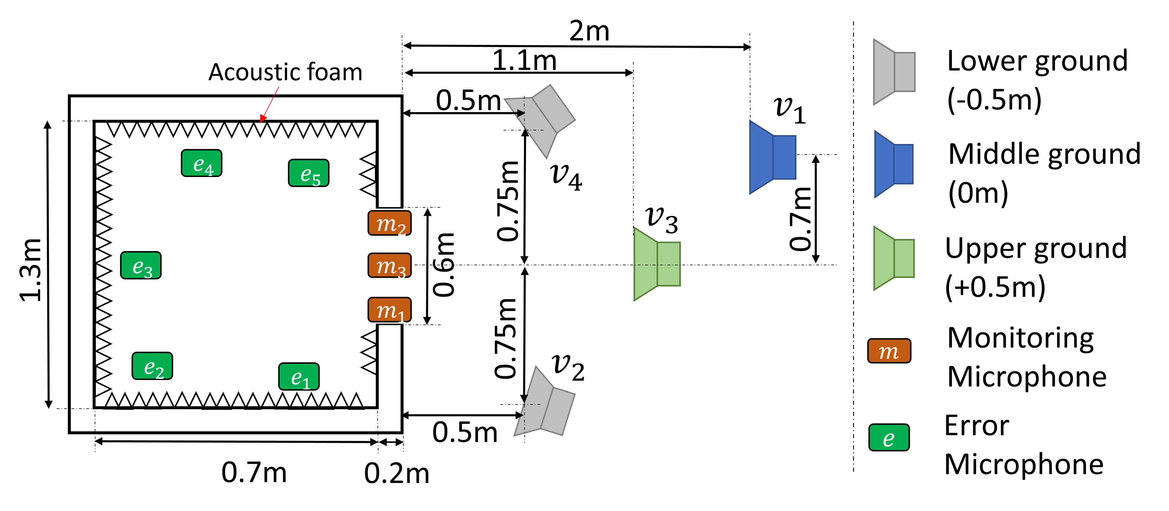
Fig. 2: Top view of the virtual sensing system for an open aperture, showing the arrangement of primary loudspeakers (Genelec 8302A) $v_{1}\;$–$\;v_{4}$, physical monitoring microphones $m_{1}\;$–$\;m_{3}$ and virtual error microphones $e_{1}\;$–$\;e_{5}$ (Pro Signal NPA415-OMNI). Signals were acquired and computed on a low-latency system (NI PXIe-8880) at a sampling frequency $F_{s}=10\text{kHz}$. [13].

As $r_{n_{v}}$ varies with time in a real-time implementation, it is important to understand the significance of this parameter. Additional real-time experiments from [13] were conducted with its arrangement shown in Fig.3. Each loudspeaker reproduced white Gaussian noise during the calibration stage to obtain the individual CMs $\mathbf{R}_{d_{m}d_{e}}^{(n_{v})}$ and $\mathbf{R}_{d_{m}d_{m}}^{(n_{v})}$, which will be used to reconstruct the OF from Eq.(5). Fig.3(a)–3(b) showed the estimation error spectra when both $v_{1}$ and $v_{2}$ reproduced known amplitude ratios. While the nominal OF $\bm{O}_{opt}$ was directly obtained from both loudspeakers with the new amplitude ratio, the correctly estimated and mismatched OF $\hat{\bm{O}}$ and $\hat{\bm{O}}_{mis}$ uses the CM obtained from the calibration stage where the original amplitude was used for each individual loudspeaker, followed by the superposition formulation from Eq.(5) using the correct and mismatched amplitude ratio input. The correctly estimated OF for both Fig.3(a) and 3(b) showed a similar estimation spectra with the nominal OF which effectively validates Eq.(5). However, the estimation error can degrade when the wrong amplitude ratio is used. While Fig.3(a) showed a decrease in estimation error at frequencies 400–600Hz, higher frequency region from 800–1000Hz did not show much change. Fig.3(b) showed a larger difference in estimation error in a wider frequency range, suggesting a larger degradation in estimation error when its mismatch becomes larger. Thus, it can be concluded that the source ratio $r_{n_{v}}$ would play an important role to achieve robust estimation.

(a) $r_{1}=1.2,r_{2}=0.8$
$r_{1,mis}=0.8,r_{2,mis}=1.2$

(b) $r_{1}=1.5,r_{2}=0.5$
$r_{1,mis}=0.5,r_{2,mis}=1.5$

Fig. 3: The estimation spectra when loudspeaker 1 and 2 as arranged from Fig.2 [13] were present, using the optimal OF $\bm{O}_{opt}$, correctly predicted OF $\hat{\bm{O}}_{opt}$ and the mismatched OF $\hat{\bm{O}}_{mis}$ calculated from Eq.(5).

4 Source tracking formulation

In RMT implementation, multiple physical monitoring microphones are typically used, and thus the true cross-correlation matrix (CCM) between monitoring microphones $\mathbf{R}_{d_{m}d_{m}}$ can be obtained. By assuming incoherence between noise sources, and each CCM associated with that noise source was measured, the estimated CCM for $\hat{\mathbf{R}}_{d_{m}d_{m}}$ can be expressed as

$$\hat{\mathbf{R}}_{d_{m}d_{m}}=\sum_{n_{v}=1}^{N_{v}}z_{n_{v}}\mathbf{R}_{d_{m}d_{m}}^{(n_{v})},$$ (6)

with its respective source ratio parameter $z_{n_{v}}=r_{n_{v}}^{2}$ derived from Eq.(5). As $\mathbf{R}_{d_{m}d_{m}}$ changes with time due to changes in $z_{n_{v}}$, the cost function can be formulated by minimizing its $l_{2}$ norm of the difference between the estimated CCM and its true CCM measured at that time. Thus, the minimization problem can be formulated as

$$\min\;J(n) = \left\|\mathbf{R}_{d_{m}d_{m}}(n)-\hat{\mathbf{R}}_{d_{m}d_{m}}(n)\right\|_{2}^{2}$$ (7)

$$s.t. \quad\mathbf{a}\leq\mathbf{z}\leq\mathbf{b}$$

where $\mathbf{z}=[z_{1}\;z_{2}\;\cdots\;z_{N_{v}}]^{T}$ is the squared source ratio vector; $\mathbf{a}=[a_{1}\;a_{2}\cdots\;a_{N_{v}}]^{T}$ and $\mathbf{b}=[b_{1}\;b_{2}\cdots\;b_{N_{v}}]^{T}$ are the element-wise positive lower and upper bound vector constraints, i.e. $a_{n},\;b_{n}\geq 0$ for all $n$. The objective function can thus be formulated with the use of the quadratic penalty function, defined as

$$Q =\left\|\mathbf{R}_{d_{m}d_{m}}-\mathbf{\hat{R}}_{d_{m}d_{m}}\right\|^{2}_{2}$$

$$+\sum_{n_{v}=1}^{N_{v}}\sigma_{n_{v}}\left[h_{n_{v}}(z_{n_{v}}-a_{n_{v}})^{2}+g_{n_{v}}(z_{n_{v}}-b_{n_{v}})^{2}\right]$$ (8)

where $\mathbf{h}=[h_{1}\;h_{2}\;\cdots\;h_{N_{v}}]^{T}$ and $\mathbf{g}=[g_{1}\;g_{2}\;\cdots\;g_{N_{v}}]^{T}$ are penalty vectors that serves as a Heaviside function if the constraints were violated, given by

$$h_{n_{v}}=\begin{cases}1,&z_{n_{v}}<a_{n_{v}}\\ 0,&\text{otherwise}\end{cases}\;,\;g_{n_{v}}=\begin{cases}1,&z_{n_{v}}>b_{n_{v}}\\ 0,&\text{otherwise}\end{cases},$$ (9)

and $\sigma_{n_{v}}$ is the penalty weight. Thus, the derivatives can be shown to be

$$\frac{\partial Q}{\partial z_{n_{v}}}= 2tr\left\{-\mathbf{R}_{d_{m}d_{m}}\mathbf{R}_{d_{m}d_{m}}^{(n_{v}),T}+\mathbf{R}_{d_{m}d_{m}}^{(n_{v})}\mathbf{\hat{R}}_{d_{m}d_{m}}^{T}\right\}$$ (10)

$$+ 2\sigma_{n_{v}}\left[(z_{n_{v}}-a_{n_{v}})h_{n_{v}}+(z_{n_{v}}-b_{n_{v}})g_{n_{v}}\right].$$

Assuming that optimal $\mathbf{z}$ remained unconstrained, i.e. $\mathbf{a}<\mathbf{z}_{opt}<\mathbf{b}\text{, and thus }\mathbf{h}=\mathbf{g}=0$, the optimal squared source ratio $\mathbf{z}_{opt}$ can be obtained by setting the derivatives to zero, that is

$$\mathbf{z}_{opt}=\mathbf{A}^{-1}\mathbf{c},$$ (11)

where

$$\mathbf{A}=\begin{bmatrix}\text{tr}\left\{\mathbf{R}_{d_{m}d_{m}}^{(1)}\mathbf{R}_{d_{m}d_{m}}^{(1),T}\right\}&\cdots&\text{tr}\left\{\mathbf{R}_{d_{m}d_{m}}^{(1)}\mathbf{R}_{d_{m}d_{m}}^{(N_{v}),T}\right\}\\ \text{tr}\left\{\mathbf{R}_{d_{m}d_{m}}^{(2)}\mathbf{R}_{d_{m}d_{m}}^{(1),T}\right\}&\cdots&\text{tr}\left\{\mathbf{R}_{d_{m}d_{m}}^{(2)}\mathbf{R}_{d_{m}d_{m}}^{(N_{v}),T}\right\}\\ \cdots&\ddots&\vdots\\ \text{tr}\left\{\mathbf{R}_{d_{m}d_{m}}^{(N_{v})}\mathbf{R}_{d_{m}d_{m}}^{(1),T}\right\}&\cdots&\text{tr}\left\{\mathbf{R}_{d_{m}d_{m}}^{(N_{v})}\mathbf{R}_{d_{m}d_{m}}^{(N_{v}),T}\right\}\end{bmatrix}$$ (12)

and

$$\mathbf{c}=\begin{Bmatrix}\text{tr}\left\{\mathbf{R}_{d_{m}d_{m}}\mathbf{R}_{d_{m}d_{m}}^{(1),T}\right\}\\ \text{tr}\left\{\mathbf{R}_{d_{m}d_{m}}\mathbf{R}_{d_{m}d_{m}}^{(2),T}\right\}\\ \vdots\\ \text{tr}\left\{\mathbf{R}_{d_{m}d_{m}}\mathbf{R}_{d_{m}d_{m}}^{(N_{v}),T}\right\}\end{Bmatrix}.$$ (13)

Since the optimal approach in Eq.(11) is unconstrained and may lead to matrix ill-conditioning with large $N_{v}$ [17], an iterative gradient descent approach is adopted, whereby

$$z_{n_{v}}^{(n+1)}= z_{n_{v}}^{(n)}-\alpha_{n_{v}}\Biggl{\{}\text{tr}\left\{\mathbf{R}_{d_{m}d_{m}}^{(n_{v})}\mathbf{\hat{R}}_{d_{m}d_{m}}^{T}-\mathbf{R}_{d_{m}d_{m}}\mathbf{R}_{d_{m}d_{m}}^{(n_{v}),T}\right\}$$

$$+ \sigma_{n_{v}}\left[(z_{n_{v}}^{(n)}-a_{n_{v}})h_{n_{v}}+(z_{n_{v}}^{(n)}-b_{n_{v}})g_{n_{v}}\right]\Biggr{\}}.$$ (14)

As $\mathbf{z}$ is being iterated closer to the optimal value, and therefore getting an accurate reconstruction of $\mathbf{R}_{d_{m}d_{m}}$, an accurate estimation of $\mathbf{R}_{d_{m}d_{e}}$ will be achieved indirectly as both correlation terms share the same source ratio term, which allows the reconstruction shown from Eq.(5) to be implemented in real-time. The normalised estimation error of the source tracking technique across the $n$-th iteration can therefore be expressed given the general form of

$$L_{xy}(n)=10\log_{10}\left(\frac{\left\|\mathbf{R}_{xy}(n)-\hat{\mathbf{R}}_{xy}(n)\right\|^{2}_{2}}{\left\|\mathbf{R}_{xy}(n)\right\|^{2}_{2}}\right)$$ (15)

where the $xy$ subscript from Eq.(15) can either be $d_{m}d_{m}$ or $d_{m}d_{e}$.

There is a distinction in this approach as compared to other traditional source-localization methods. Unlike the conventional CMF approach or DAMAS that makes use of a steering vector [14], this method does not assume a free-field propagation from the noise source to the microphones which allows us to obtain the source ratio in a diffuse field. While it is certainly comparable to the acoustic inverse method [15], this formulation strictly assumes that the noise source clusters are incoherent as explained in Section 3. Additionally, the time domain CM is used instead of the cross-spectral density (CSD) in the frequency domain in this formulation which allows the causally constrained time-domain observation filter from Eq.(5) to be reconstructed. This method, therefore, is well suited for certain virtual sensing applications, such as separating road noise and wind noise in automobile ANC as the CM caused by the road noise and wind noise can be measured separately.

5 Simulation results

(a)

(b)

Fig. 4: The plot of (4(a)): Source ratio and (4(b)): Source-tracking estimation error from Eq.(15) over time using previous measurements from [13]. $\alpha$ = 5, $\mathbf{a}=0$ and $\mathbf{b}=5$ were used in this simulation, and the exact source-ratio used for each loudspeakers are $\mathbf{z}=1$. The true correlation matrix $\mathbf{R}_{d_{m}d_{m}}$ with the length of 400 is obtained for every time-frame of 200 samples (overlap of 50%).

To verify the proposed algorithm in Section 4, simulations were made on the VS system in the case where all four primary loudspeakers from Fig.2 were present with a given source ratio parameter of 1, but the source ratio parameters were iterated along sample frame using Eq.(14). Fig.4(a)–4(b) show the iteration plot of the source ratio parameter and the normalised source-tracking estimation error over a period of 10 seconds using Eq.(14) and Eq.(15). The iteration plot of the source ratio parameter showed convergence for all noise sources to around 1, with $r_{1}$ and $r_{3}$ converging quicker than $r_{2}$ and $r_{4}$. As the true $\mathbf{R}_{d_{m}d_{m}}$ with a length of 400 and overlap of 50% has been obtained throughout the time frame, it is expected for the source ratio parameter to have random fluctuations from its stochastic nature, thus validating Eq.(14) from obtaining its source ratio parameter. This convergence is also supported in Fig.4(b) where $L_{d_{m}d_{m}}$ converges to around -13dB with expected random fluctuations. Interestingly, the estimation error of $\mathbf{R}_{d_{m}d_{e}}$ has decreased with time and converges at about -10dB even if it’s indirectly estimated, which verifies the estimation concept described in Section 4 where a good correlation in $L_{d_{m}d_{m}}$ and $L_{d_{m}d_{e}}$ is shown in Fig.4(b). Once $\mathbf{z}$ has been found through iteration, the observation filter due to source-tracking algorithm $\hat{\bm{O}}_{st}$ will be iteratively updated and was used to simulate the estimated error signals. It has been shown from the estimation error plot from Fig.5 that the estimation spectra between the nominal observation filter $\bm{O}_{opt}$ and source tracking observation filter $\hat{\bm{O}}_{st}$, which ultimately verifies the source-tracking algorithm.

Fig. 5: The estimation error spectra when all 4 loudspeakers from Fig.2 were present, using the optimal observation filter $\bm{O}_{opt}$, estimated observation filter $\hat{\bm{O}}$ with $\mathbf{z}=1$ and estimated observation filter with the use of source tracking iteration $\hat{\bm{O}}_{st}$.

6 Conclusion

Although the remote microphone technique is sensitive to changes in the primary acoustic field, it can be reconstructed in real-time implementation through source decomposition as shown previously. The effect of the source ratio parameter on the estimation performance, however, is yet to be studied. In this paper, we have demonstrated the significance of the source ratio parameter when performing the RMT through source decomposition, as a large mismatch in the source ratio will cause a degradation of the estimation. Thus, we proposed a source-tracking algorithm by matching the CM directly and then iterating the source ratio parameter through gradient descent. To verify our algorithm, simulations with physical measurements from an open-aperture setup were conducted. Simulation results showed a good convergence when estimating the source ratio using the proposed algorithm, and thus can be used to reconstruct the observation filter in real-time implementation.

References

- [1] Danielle Moreau, Ben Cazzolato, Anthony Zander, and Cornelis Petersen, “A review of virtual sensing algorithms for active noise control,” Algorithms, vol. 1, no. 2, pp. 69–99, 2008.
- [2] Shoma Edamoto, Chuang Shi, and Yoshinobu Kajikawa, “Virtual Sensing Technique for Feedforward Active Noise Control,” in 171st Meeting of the Acoustical Society of America, Salt Lake City, Utah, 2016, p. 030001.
- [3] He-Siang Deng, Cheng-Yuan Chang, and Sen M. Kuo, “Active Noise Control with Virtual Sensing Technology for Headrest,” in 2018 Asia-Pacific Signal and Information Processing Association Annual Summit and Conference (APSIPA ASC), Honolulu, HI, USA, Nov. 2018, pp. 1272–1275, IEEE.
- [4] Huiyuan Sun, Jihui Zhang, Thushara Abhayapala, and Prasanga Samarasinghe, “Spatial Active Noise Control with the Remote Microphone Technique: An Approach with a Moving Higher Order Microphone,” in ICASSP2022, 2022, p. 5.
- [5] Stephen J. Elliott and Jordan Cheer, “Modeling local active sound control with remote sensors in spatially random pressure fields,” The Journal of the Acoustical Society of America, vol. 137, no. 4, pp. 1936–1946, 2015.
- [6] Stephen J. Elliott, Jin Zhang, Chung Kwan Lai, and Jordan Cheer, “Superposition of the uncertainties in acoustic responses and the robust design of active control systems,” The Journal of the Acoustical Society of America, vol. 148, no. 3, pp. 1415–1424, 2020.
- [7] Jin Zhang, Stephen J. Elliott, and Jordan Cheer, “Robust performance of virtual sensing methods for active noise control,” Mechanical Systems and Signal Processing, vol. 152, pp. 107453, 2021.
- [8] Woomin Jung, Stephen J. Elliott, and Jordan Cheer, “Estimation of the pressure at a listener’s ears in an active headrest system using the remote microphone technique,” The Journal of the Acoustical Society of America, vol. 143, no. 5, pp. 2858–2869, 2018.
- [9] Stephen J. Elliott, Woomin Jung, and Jordan Cheer, “Head tracking extends local active control of broadband sound to higher frequencies,” Scientific Reports, vol. 8, no. 1, pp. 5403, Dec. 2018.
- [10] Dongyuan Shi, Woon-Seng Gan, Bhan Lam, Rina Hasegawa, and Yoshinobu Kajikawa, “Feedforward multichannel virtual-sensing active control of noise through an aperture: Analysis on causality and sensor-actuator constraints,” The Journal of the Acoustical Society of America, vol. 147, no. 1, pp. 32–48, 2020.
- [11] Bhan Lam, Dongyuan Shi, Woon Seng Gan, Stephen J. Elliott, and Masaharu Nishimura, “Active control of broadband sound through the open aperture of a full-sized domestic window,” Scientific Reports, vol. 10, no. 1, pp. 1–7, 2020.
- [12] Jordan Cheer, Stephen J. Elliott, Eunmi Oh, and Jonghoon Jeong, “Application of the remote microphone method to active noise control in a mobile phone,” The Journal of the Acoustical Society of America, vol. 143, no. 4, pp. 2142–2151, Apr. 2018.
- [13] Chung Kwan Lai, Bhan Lam, Jing Sheng Tey, and Woon Seng Gan, “Robust estimation of open aperture active control systems using virtual sensing,” in Internoise 2022, Aug. 2022, p. 11.
- [14] Tarik Yardibi, Nikolas S Zawodny, Chris Bahr, Fei Liu, Louis N Cattafesta, and Jian Li, “Comparison of Microphone Array Processing Techniques for Aeroacoustic Measurements,” International Journal of Aeroacoustics, vol. 9, no. 6, pp. 733–761, July 2010.
- [15] P.A. Nelson and S.H. Yoon, “Estimation of Acoustic Source Strength by Inverse Methods: Part I, Conditioning of the Inverse Problem,” Journal of Sound and Vibration, vol. 233, no. 4, pp. 639–664, June 2000.
- [16] Woomin Jung, Stephen J. Elliott, and Jordan Cheer, “Local active control of road noise inside a vehicle,” Mechanical Systems and Signal Processing, vol. 121, pp. 144–157, 2019.
- [17] Tarik Yardibi, Jian Li, Petre Stoica, Nikolas S. Zawodny, and Louis N. Cattafesta, “A covariance fitting approach for correlated acoustic source mapping,” The Journal of the Acoustical Society of America, vol. 127, no. 5, pp. 2920–2931, May 2010.