Measuring Agreement Among Several Raters Classifying Subjects Into One-Or-More (Hierarchical) Nominal Categories. A Generalisation of Fleiss’ kappa

Abstract

Cohen’s and Fleiss’ kappa are well-known measures for inter-rater reliability. However, they only allow a rater to select exactly one category for each subject. This is a severe limitation in some research contexts: for example, measuring the inter-rater reliability of a group of psychiatrists diagnosing patients into multiple disorders is impossible with these measures. This paper proposes a generalisation of the Fleiss’ kappa coefficient that lifts this limitation. Specifically, the proposed $\kappa$ statistic measures inter-rater reliability between multiple raters classifying subjects into one-or-more nominal categories. These categories can be weighted according to their importance, and the measure can take into account the category hierarchy (e.g., categories consisting of subcategories that are only available when choosing the main category like a primary psychiatric disorder and sub-disorders; but much more complex dependencies between categories are possible as well). The proposed $\kappa$ statistic can handle missing data and a varying number of raters for subjects or categories. The paper briefly overviews existing methods allowing raters to classify subjects into multiple categories. Next, we derive our proposed measure step-by-step and prove that the proposed measure equals Fleiss’ kappa when a fixed number of raters chose one category for each subject. The measure was developed to investigate the reliability of a new mathematics assessment method, of which an example is elaborated. The paper concludes with the worked-out example of psychiatrists diagnosing patients into multiple disorders.

Keywords Inter-rater reliability $\cdot$ Fleiss’ kappa  $\cdot$ Multiple categories $\cdot$ Hierarchical categories  $\cdot$ Weighted categories

1 Introduction

Inter-rater reliability is the degree of agreement among independent observers who rate, code, or assess the same phenomenon. These ratings often rely on subjective evaluations provided by human raters, who sometimes differ greatly from one rater to another (Gwet, 2012; Vanacore  Pellegrino, 2022). Various researchers in many different scientific fields have recognized this problem for a long time since science requires measurements to be reproducible and accurate. Ideally, only a change in the subject’s attribute should cause variation in the ratings, while the rater-induced source of variation should be excluded as it can jeopardize the integrity of scientific inquiries. The resolution to these problems, or at least the measurement of how big these problems are, is the study of inter-rater reliability.

1.1 Cohen’s kappa

Starting from the 1950s, various inter-rater reliability measures have been proposed (Osgood, 1959; Bennett ., 1954), from which Cohen’s kappa (Cohen, 1960) is the most well-known chance-corrected measure. This correction for chance is essential, as two raters may agree by following a clear, deterministic rating procedure, or they may agree by chance (Gwet, 2012). Thus, by accounting for chance, the kappa coefficient takes into account the difficulty of the classification task at hand. The formula of Cohen’s kappa (Cohen, 1960) is:

$$\kappa=\frac{Po-Pe}{1-Pe},$$ (1)

where $Po$ is the observed agreement and $Pe$ is the expected agreement by chance. Cohen (1960) calls the nominator the beyond-chance: by subtracting the observed agreement with the expected agreement by chance, you are left with ‘the percent of units in which beyond-chance occurred’; the denominator $1-Pe$ can be seen as the ‘beyond-chance’ in the case of perfectly agreeing raters (the observed agreement is replaced with 1). So the kappa-statistic is the proportion of the observed beyond-chance over the beyond-chance in an ideal world of perfectly agreeing raters. Hence, the $\kappa$-coefficient is the proportion of agreement after chance agreement is removed from consideration. $\kappa$-coefficients always vary between $-1$ and $1$, with 1 indicating perfect agreement ($Po=1$), 0 indicating no agreement better than chance ($Pe=Po$), and a value below zero indicates the agreement was less than one would expect by chance ($Po<Pe$). The exact formulas for $Po$ and $Pe$ for the Cohen’s kappa can be found in Cohen (1960).

1.2 Fleiss’ kappa

Cohen’s kappa only allows to measure agreement between two independent raters, that is why Fleiss came up with the Fleiss’ kappa in 1971 allowing a fixed number of 2 raters or more. These raters categorise subjects into exactly one of the available categories. We will now present how Fleiss defined $Po$ and $Pe$. Let $I$ be the total number of subjects, $J$ is the (fixed) number of raters and $C$ is the number of categories. Let $x_{ic}$ be the number of raters who classified the $i$-th subject ($i\in\{1,\ldots,I\}$) into the $c$-th category ($c\in\{1,\ldots C\}$). Since the categories are mutually exclusive, we know that every subject $i$ will have received exactly $J$ classifications, so $\sum_{c}x_{ic}=J$. We start with the observed agreement $P_{o}$. The extent of agreement among $J$ raters for the subject $i$ can be calculated as the proportion of agreeing rater pairs ${x_{ic}\choose 2}$ out of all the ${J\choose 2}$ possible rater pairs. This proportion $P_{i}$ for a subject $i$ can thus be defined as:

$$P_{i} =\sum_{c}\frac{{x_{ic}\choose 2}}{{J\choose 2}}$$ (2)

$$=\sum_{c}\frac{x_{ic}(x_{ic}-1)}{J(J-1)}$$

$$=\frac{\sum_{c}x_{ic}^{2}-J}{J(J-1).}$$

The overall observed proportion of agreement $P_{o}$ may then be measured by the mean of all $P_{i}$’s, so:

$$P_{o} =\frac{1}{I}\sum_{i}P_{i}$$

$$=\frac{\sum_{i}\sum_{c}x_{ic}^{2}-IJ}{IJ(J-1)}.$$ (3)

We now turn to the formula of $P_{e}$, the expected agreement by chance. In total, $IJ$ classifications will have been performed: all raters select exactly 1 category for each subject. So, the proportion of all assignments to the $c$-th category can be expressed as $\frac{\sum_{i}x_{ic}}{IJ}$, this is thus the probability to assign a subject to category $c$ by chance. Consequently, the probability that any pair of (independent) raters classify a subject into category $c$ by chance is given by $\left(\frac{\sum_{i}x_{ic}}{IJ}\right)^{2}$. Hence, if the raters made their classifications purely at random, the probability that two raters agree by chance on all categories is given by:

$$P_{e} =\sum_{c}\left(\frac{\sum_{i}x_{ic}}{IJ}\right)^{2},$$ (4)

Plugging the above formulas into the $\kappa$ statistic expressed in (1), gives the Fleiss’ kappa:

$$\kappa=\frac{\frac{\sum_{i}\sum_{c}x_{ic}^{2}-IJ}{IJ(J-1)}-\sum_{c}\left(\frac{\sum_{i}x_{ic}}{IJ}\right)^{2}}{1-\sum_{c}\left(\frac{\sum_{i}x_{ic}}{IJ}\right)^{2}}.$$ (5)

A more elaborate description and an example of psychiatric diagnosis on 30 subjects by six raters into a single disorder category, can be found in Fleiss (1971).

1.3 Paradoxes

Although both Cohen’s kappa and Fleiss’ kappa are widely popular measures for inter-rater reliability, some scholars have pointed out that these kappa coefficients are not free from paradoxes and can occasionally yield unexpected results (Warrens, 2010; Gwet, 2008; Feinstein  Cicchetti, 1990). One paradox arises when both the observed agreement $Po$ and the expected chance agreement $Pe$ are high: the correction process embodied in kappa’s formula (see (1)) can return a relatively low or even negative value of $\kappa$, whilst the observed agreement $Po$ is high. Another paradox is known as the prevalence paradox: it can be shown that the probabilities $\frac{\sum_{i}x_{ic}}{IJ}$ produce higher $\kappa$-values when they are more balanced, i.e. when all categories are used about equally often and no particularly common categories exist. According to Gwet (2012), these probabilities are not suited to correctly measure the expected chance agreement $Pe$. All ratings for each category are used in the calculation of $Pe$, but as we want to say something about expected chance agreement, this philosophically implies we treat all these ratings as if they were all assigned randomly, which, according to Gwet (2012), is an unacceptable premise. Kraemer . (2002) disagree with Gwet’s view, saying that ‘it is well known that it is very difficult to achieve high reliability of any measure in a very homogeneous population (of subjects).’

1.4 Other methods

The literature on chance-corrected inter-rater reliability measures boomed in the 1970s and 1980s, with many proposals for different measures for different research settings. Surprisingly, only a few papers consider the limitation of mutually exclusive categories. This section briefly overviews the alternative methods in which a rater can classify a subject into multiple categories. Most of the methods below were described by Mezzich . (1981) but lacked sound mathematical expressions, which are added in this section.

1.4.1 Averaging or pooling Cohen’s kappas

To calculate the inter-rater reliability among 2 raters who can classify subjects into multiple categories, a commonly used method is to calculate a Cohen’s kappa (Cohen, 1960) for each category and average them: $\overline{\kappa}$. A problem with this approach is that when a category has an undefined Cohen’s $\kappa$, $\overline{\kappa}$ is undefined too (which happens if the expected agreement by chance $Pe$ is $1$, e.g. when any rater did not select the category). A solution for this is pooling the Cohen’s kappas by calculating the $Po$ and $Pe$ for each category separately and then taking the average $\overline{Po}$ and $\overline{Pe}$. Next, these averages are plugged in (1).

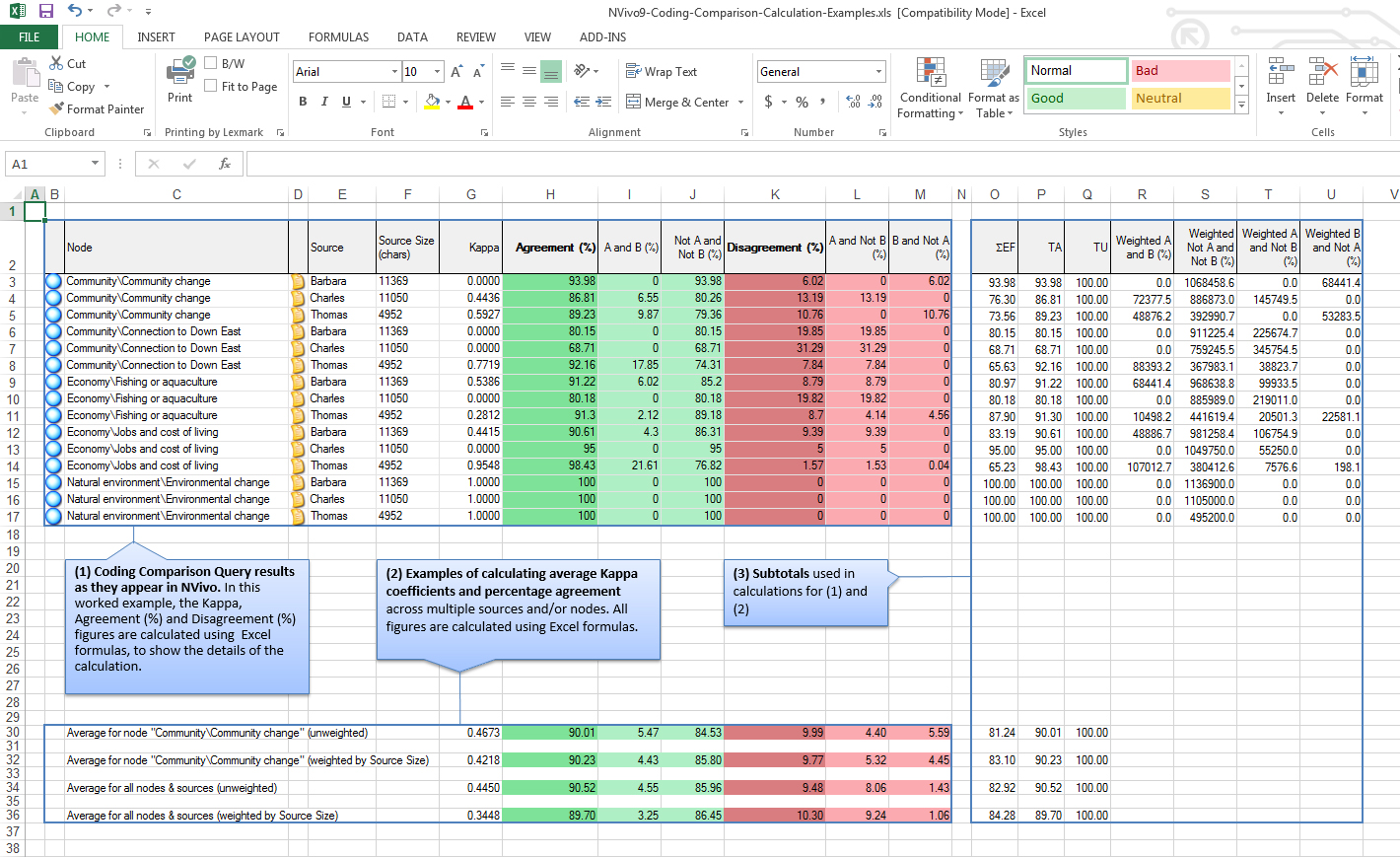
Figure 1: NVivo advocates the pooled Cohen’s kappa approach in the provided Excel sheets to get an overall $\kappa$ of the coding process.

For example, NVivo (2022) - a popular program for qualitative research - advocates the pooled Cohen’s kappa to measure the inter-rater reliability among two coders. These two coders (= ‘raters’) can code in NVivo the different sources (= ‘subjects’) of their research (e.g. text fragments, interviews, pictures) to one-or-more nodes of their codebook (= ‘categories’). To get an overall $\kappa$ of this coding process, Cohen’s kappa is not suited: it would only allow the coders to code a source to exactly one node in their codebook. In contrast, a source is often coded to various nodes of the codebook. Therefore, Cohen’s kappa is calculated for each node in the codebook separately, and the pooled Cohen’s kappa is used to get an overall $\kappa$ of the coding process (Figure 1).

In 2008, De Vries . published a simulation study in which they compared ‘true’ Cohen’s kappa values with the (simulated) averaged kappa and the (simulated) pooled kappa. Results showed that the pooled kappa almost always deviates less from the true kappa than the averaged kappa, resulting in smaller root-mean-square errors. Especially if the expected agreement by chance $Pe$ is 0.6 or higher, the pooled Cohen’s kappa outperforms the averaged Cohen’s kappa. Indeed, when $Pe$ is large, the denominator of the corresponding Cohen’s kappa is small. In the case of the averaged kappa, the denominator of individual kappas has a multiplicative effect on the outcome (the numerator has an additive effect), making the method less precise when some individual denominators become small.

An important constraint to averaging or pooling Cohen’s kappas is embodied in the formulas of Cohen’s kappa itself: while the limitation of only one category for each subject is lifted, it is still limited to measure inter-rater reliability among exactly 2 raters.

1.4.2 Proportional overlap

The proportional overlap method was first introduced by Mezzich . in 1981. The method allows the calculation of a $\kappa$ statistic in which multiple raters can classify subjects into multiple categories. The proportional overlap $\kappa$ is calculated between pairs of raters. Let $A_{ij}$ be the set of categories selected by rater $j$ for subject $i$. The proportion of agreement between two raters $a$ and $b$ is then defined as the ratio of $\#(A_{ia}\cap A_{ib})$ (= the number of categories that were selected by both raters $a$ and $b$ for subject $i$) over $\#(A_{ia}\cup A_{ib})$ (= the total number of categories selected by rater $a$ or $b$ for subject $i$). For example, if rater $a$ selected categories $\{$blue, yellow, brown$\}$ and rater $b$ selected $\{$blue, green$\}$ for a given subject $i$, their proportional overlap is the ratio of 1 (one agreement on ‘blue’) over 4 (in total, rater $a$ and $b$ selected 4 different categories for subject $i$: blue, yellow, brown and green), so we get a proportional overlap of $0.25$. In general, the proportional overlap ranges between 0 (= no overlap between the selected categories) and 1 (= perfect agreement, all categories match).

Agreement among several raters for a given subject is measured by averaging the proportions of agreement obtained for all combinations of pairs of raters for that subject. The overall observed proportion of agreement $Po$ is the average of the mean proportions of agreement obtained for each of the $I$ subjects in the sample:

$$P_{o}=\frac{\sum_{i}\sum_{(a,b)\in{J\choose 2}}\frac{\#(A_{ia}\cap A_{ib})}{\#(A_{ia}\cup A_{ib})}}{I\frac{J(J-1)}{2}}\quad\text{with }(a,b)\in\mathbb{N}^{2}$$ (6)

To determine the proportion of chance agreement $Pe$, compute the proportions of agreement between all combinations of classifications $A_{ij}$ for all raters and all subjects, and take the average. This can easily be done by using software and looping over all these combinations. Mathematically, the rather complex formula can be expressed as follows:

$$P_{e}=\frac{\sum_{(x,y)\in{I\cdot J\choose 2}}\frac{\#\left[A_{\lceil x/J\rceil,(x-1\text{ mod }J)+1}\bigcap A_{\lceil y/J\rceil,(y-1\text{ mod }J)+1}\right]}{\#\left[A_{\lceil x/J\rceil,(x-1\text{ mod }J)+1}\bigcup A_{\lceil y/J\rceil,(y-1\text{ mod }J)+1}\right]}}{\frac{IJ(IJ-1)}{2}}\quad\text{with }(x,y)\in\mathbb{N}^{2}$$ (7)

To understand the above formula, imagine an $I\times J$-grid where each cell represents the classifications $A_{ij}$ of subject $i$ by rater $j$. This $I\times J$-grid contains $I\cdot J$ cells that can be numbered row by row. An example with 3 subjects and 4 raters is given in Table 1. The last cell will have number $I\cdot J$. Now, take a pair $(x,y)$ out of the possible combinations of two numbers from 1 to $I\cdot J$. Both $x$ and $y$ refer to a cell in the numbered $I\times J$-grid. We need to translate $x$ (and $y$) back to the corresponding subject and rater. To find the subject, take the ceiling of the division of $x$ by $J$ $(=\lceil x/J\rceil)$. To find the rater, take $x-1$ module $J$ and add 1.

Table 1: Numbering an $I\times J$-grid of classifications $A_{ij}$

	Rater 1	Rater 2	Rater 3	Rater 4			Rater 1	Rater 2	Rater 3	Rater 4
Subject 1	$A_{11}$	$A_{12}$	$A_{13}$	$A_{14}$	$\rightarrow$	Subject 1	1	2	3	4
Subject 2	$A_{21}$	$A_{22}$	$A_{23}$	$A_{24}$		Subject 2	5	6	7	8
Subject 3	$A_{31}$	$A_{32}$	$A_{33}$	$A_{34}$		Subject 3	9	10	11	12

As a number example with 3 subjects and 4 raters (Table 1), take the pair $(10,12)$. To find the subject belonging to $10$, we calculate $\lceil 10/4\rceil=\lceil 2.5\rceil=3$, so we get subject $3$. To find the rater belonging to 12, we calculate $(12-1)\text{ mod }4=11\text{ mod }4=3$ and add $1$, so we get rater $4$.

The corresponding ‘Mezzich’s $\kappa$’ is found by plugging in $Po$ and $Pe$ in Cohen’s formula (1).

The proportional overlap method is an intuitive way to handle multiple raters classifying subjects into one-or-more categories and is easy to adapt to a varying number of raters (cf. some combinations of raters will not be presented in this case). However, the method has limitations: it can not handle different weights for categories, nor category hierarchies. Moreover, the calculation of $Pe$ depends on the number of combinations ${I\cdot J\choose 2}$, which makes computation very demanding if the number of subjects $I$ or the number of raters $J$ is high. Using a random sample of combinations might solve the computational issue, but it is an open question how large this random sample should be to guarantee sufficient accuracy.

1.4.3 Chance-corrected intraclass correlations

Mezzich . (1981) also proposed a method to use intraclass correlation coefficients as an intermediate step for the determination of a kappa statistic to allow the selection of multiple categories for each subject by multiple raters. To calculate the intraclass correlations, let $\mathbf{x_{ij}}=(x_{ij1},x_{ij2},\ldots,x_{ijC})$ represent the classification vector of the $i$-th subject ($i\in\{1,\ldots,I\}$) for the $j$-th rater ($j\in\{1,\ldots,J\}$), with $x_{ijc}=1$ when subject $i$ was classified by rater $j$ into category $c$ ($c\in\{1,\ldots C\}$), and $x_{ijc}=0$ otherwise. A measure of agreement is obtained by computing an intraclass correlation coefficient $\rho_{i}$ between all $\mathbf{x_{ij}}$ for a given subject $i$ for all raters using a one-way ANOVA. If all the raters classified subject $i$ in the same categories, perfect agreement is obtained, $\rho_{i}=1$. $Po$ can be computed by taking the average of $\rho_{1},\rho_{2},\ldots,\rho_{I}$. $Pe$ is determined by computing the intraclass correlation coefficient between all classification vectors $\mathbf{x_{ij}}$ for all raters and all subjects. Plugging $Po$ and $Pe$ in (1) gives the value of the ‘chance-corrected intraclass correlations.’ Although the method is powerful by it simplicity, it can not handle different weights for categories, nor category hierarchies.

1.4.4 Chance-corrected rank correlations

The method proposed by Kraemer in 1980 is the only method we found in the literature were multiple raters classify subjects into an ordered lists of categories: e.g., the best-fitting category for the subject according to the rater is ranked first, the second best-fitting category second, etc.

To calculate the corresponding kappa statistic, Kraemer uses classification vectors $\mathbf{x^{\prime}_{ij}}$ that contain ranks of the classifications drafted by rater $j$ for subject $i$. For example, if for a given subject $i$, rater $j$ made an ordered list of $k$ categories ($k\leq C$), a 1 is assigned to the first category mentioned, a 2 to the second category, etc. Finally, categories that were not on the ordered list of rater $j$ for subject $i$ get rank $\frac{C+k+1}{2}$ assigned in vector $\mathbf{x_{ij}}$, which equals the average of the remaining ranks. If raters can not decide the order between some selected categories, tied ranks can be placed in vector $\mathbf{x^{\prime}_{ij}}$.

Assume, for example, that rater $j$ made the following ordered classifications for subject $i:$ 1. green 2. brown 2. orange 2. red 3. yellow., based on the 8 available categories $\{$blue, brown, green, pink, purple, orange, red, yellow$\}$ . Then, green would have a rank of 1, and brown, orange and red get rank 3 (i.e., the average of the ranks $2,3,4$). Yellow receives rank 5. The unchosen categories (blue, pink, purple) get rank $\frac{8+5+1}{2}=7$ (i.e., average of the remaining ranks $6,7$ and $8$). The resulting $\mathbf{x^{\prime}_{ij}}$ equals $(7,3,1,7,7,3,3,5)$.

The chance-corrected rank correlations $\kappa$ is calculated between pairs of raters. In this case, the Spearman correlation coefficient measures the agreement between two ranked classification vectors. Perfect agreement is obtained only if the two vectors are exactly the same. Let $r_{i}$ be the average Spearman correlation coefficient between all pairs of raters for subject $i$, then $Po$ is the average of $r_{1},\ldots,r_{I}$:

$$P_{o}=\frac{\sum_{i}\sum_{(a,b)\in{J\choose 2}}r_{\mathbf{x_{ia}},\mathbf{x_{ib}}}}{I\frac{J(J-1)}{2}}$$ (8)

$Pe$ is calculated by averaging the Spearman correlation coefficient among all pairs of raters, for all subjects:

$$P_{e}=\frac{\sum_{(c,d)\in{I\cdot J\choose 2}}r_{\mathbf{x_{\lceil c/J\rceil,(c-1\text{ mod }J)+1}},\mathbf{x_{\lceil d/J\rceil,(d-1\text{ mod }J)+1}}}}{\frac{IJ(IJ-1)}{2}}$$ (9)

The corresponding $\kappa$ is found by plugging in $Po$ and $Pe$ in Cohen’s formula (1). While the method is the only chance-corrected inter-rater reliability measure known in the literature allowing ranked classifications from raters, it can not handle different weights for categories nor category hierarchies. However, these probably do not appear in ranked classifications. The computational intensity for calculating $Pe$ is the same as in the proportional overlap method.

2 Derivation of the proposed $\kappa$ statistic

2.1 Non-hierarchical categories

Suppose a sample of $I$ subjects has been classified by the same set of $J$ raters into $C$ categories. The $C$ categories are not mutually exclusive: a subject can be classified by a rater into multiple categories. Let $\mathbf{x_{ij}}=(x_{ij1},x_{ij2},\ldots,x_{ijC})$ represent the classification vector of the $i$-th subject ($i\in\{1,\ldots,I\}$) for the $j$-th rater ($j\in\{1,\ldots,J\}$), with $x_{ijc}=1$ when subject $i$ was classified by rater $j$ into category $c$ ($c\in\{1,\ldots C\}$), and $x_{ijc}=0$ otherwise. Let $x_{ic}=\sum_{j}x_{ijc}$ denote the number of raters classifying subject $i$ into category $c$, with $J-x_{ic}$ representing the number of raters that did not classify subject $i$ into category $c$. We can assemble all $x_{ic}$’s in an $I\times C$-matrix $X$, containing all classifications. Some scholars would call $X$ the ‘agreement table.’

Furthermore, consider a weight vector $\mathbf{w}=(w_{1},\ldots,w_{C})$ where $w_{c}$ indicates the relative importance of category $c$ proportional to the weights of the other categories. The choice of $\mathbf{w}$ depends entirely on the research context in which the ratings took place. It is often conceptually convenient to impose $\sum_{c}w_{c}=1$, but this is not required. In the unweighted case where all categories are equally important, we can take both $w_{c}=\frac{1}{C},\forall c$ as well as $w_{c}=1,\forall c$.

In case the categories are non-hierarchical, the selection of a category is independent from the (non-)selection of the other categories. Intuitively, we first derive a kappa statistic like the one described by Cohen (1960) for each category $c$:

$$\kappa_{c}=\frac{Po_{c}-Pe_{c}}{1-Pe_{c}},$$ (10)

where $Po_{c}$ is the observed agreement for category $c$ and $Pe_{c}$ is the proportion of agreement expected by chance for category $c$.

We will calculate $Po_{c}$ pairwise (Conger, 1980). Two raters $a$ and $b$ agree on subject $i$ when they both classified subject $i$ into category $c$ (so $x_{iac}=x_{ibc}=1$) or when they both did not classify subject $i$ into category $c$ (so $x_{iac}=x_{ibc}=0$). Hence, the extent of agreement for subject $i$ and category $c$, can be seen as the proportion of rater pairs with agreement for category $c$ to the total number of rater pairs. So, for subject $i$ and category $c$, the nominator exists of the sum of ${x_{ic}\choose 2}$ and ${J-x_{ic}\choose 2}$, while the denominator is the amount of all possible rater pairs ${J\choose 2}$. The proportion $P_{ic}$ that denotes the extent of agreement for subject $i$ and category $c$ can thus be defined as:

$$P_{ic} =\frac{{x_{ic}\choose 2}+{J-x_{ic}\choose 2}}{{J\choose 2}}$$ (11)

$$=\frac{(x_{ic})(x_{ic}-1)+(J-x_{ic})(J-x_{ic}-1)}{J(J-1)}$$ (12)

$$=\frac{2x^{2}_{ic}-2Jx_{ic}+J^{2}-J}{J(J-1)}.$$ (13)

The overall observed proportion of agreement $Po_{c}$ for category $c$ may then be measured by taking the mean of all $P_{ic}$’s so:

$$Po_{c} =\frac{1}{I}\sum_{i}P_{ic}$$ (14)

$$=\sum_{i}\frac{2x^{2}_{ic}-2Jx_{ic}+J^{2}-J}{IJ(J-1)}.$$ (15)

$Pe_{c}$ denotes the probability that two raters agree on (not) selecting category $c$ by chance. For each category $c$, $IJ$ decisions of (not) selecting $c$ will have been performed. As $x_{ic}$ denotes the number of raters classifying subject $i$ into category $c$, $\sum_{i}x_{ic}$ represent the total number of classifications into category $c$. Hence, the proportion $\frac{\sum_{i}x_{ic}}{IJ}$ equals the probability that a rater randomly classifies a subject into category $c$. In case of two (independent) raters, the probability that both raters classify a subject into category $c$ by chance is thus $\left(\frac{\sum_{i}x_{ic}}{IJ}\right)^{2}$. If $x_{ic}$ raters classified subject $i$ into category $c$, $J-x_{ic}$ raters did not. As such, the proportion $\frac{\sum_{i}(J-x_{ic})}{IJ}$ represents the probability that a rater did not classify a subject into category $c$ by chance. In case of two (independent) raters, the probability that both raters did not classify a subject into category $c$ by chance is thus $\left(\frac{\sum_{i}(J-x_{ic})}{IJ}\right)^{2}$. Hence, the probability that two raters agree on (not) selecting category $c$ by chance equals:

$$Pe_{c} =\left(\frac{\sum_{i}x_{ic}}{IJ}\right)^{2}+\left(\frac{\sum_{i}(J-x_{ic})}{IJ}\right)^{2}$$ (16)

$$=\left(\frac{\sum_{i}x_{ic}}{IJ}\right)^{2}+\left(\frac{IJ-\sum_{i}x_{ic}}{IJ}\right)^{2}$$

$$=\left(\frac{\sum_{i}x_{ic}}{IJ}\right)^{2}+\frac{I^{2}J^{2}-2\cdot IJ\cdot\sum_{i}x_{ic}+(\sum_{i}x_{ic})^{2}}{I^{2}J^{2}}$$

$$=2\left(\frac{\sum_{i}x_{ic}}{IJ}\right)^{2}-2\left(\frac{\sum_{i}x_{ic}}{IJ}\right)+1$$ (17)

We now aggregate all $Po_{1},\ldots,Po_{C}$ and $Pe_{1},\ldots,Pe_{C}$ into one kappa-statistic, including each category according to their weights $w_{c}$:

$$\kappa=\frac{\displaystyle\sum_{c}w_{c}(Po_{c}-Pe_{c})}{\displaystyle\sum_{c}w_{c}(1-Pe_{c})}.$$ (18)

If $\sum_{c}w_{c}=1$ is imposed, this reduces to:

$$\kappa=\frac{\displaystyle\sum_{c}w_{c}Po_{c}-\sum_{c}w_{c}Pe_{c}}{1-\displaystyle\sum_{c}w_{c}Pe_{c}}.$$

2.1.1 The proposed $\kappa$ statistic is a generalisation of Fleiss’ kappa

When the requirements of the Fleiss’ kappa are fulfilled, our proposed $\kappa$-static reduces to it:

Theorem 1.

In case of equally weighted, mutually exclusive and non-hierarchical categories, the proposed kappa-statistic in (18) reduces to the Fleiss’ kappa.

Proof.

As the categories are mutually exclusive, we know that $\sum_{c}x_{ijc}=1$ for every combination of $i$ and $j$. Hence:

$$\sum_{i}\sum_{c}x_{ic}=\sum_{i}\sum_{c}\sum_{j}x_{ijc}=\sum_{i}\sum_{j}1=IJ.$$ (19)

Because the categories are equally weighted, take $w_{c}=\frac{1}{C}$ for equally weighted categories, so we get:

$$\kappa=\frac{\displaystyle\sum_{c}\frac{1}{C}(Po_{c}-Pe_{c})}{\displaystyle\sum_{c}\frac{1}{C}(1-Pe_{c})}=\frac{\displaystyle\sum_{c}(Po_{c}-Pe_{c})}{\displaystyle\sum_{c}(1-Pe_{c})}.$$

First, we rewrite the denominator. Based on (17) and (19) we get that:

$$\sum_{c}(1-Pe_{c}) =\sum_{c}\left(1-2\left(\frac{\sum_{i}x_{ic}}{IJ}\right)^{2}+2\left(\frac{\sum_{i}x_{ic}}{IJ}\right)-1\right)$$

$$=-2\sum_{c}\left(\frac{\sum_{i}x_{ic}}{IJ}\right)^{2}+2\sum_{c}\left(\frac{\sum_{i}x_{ic}}{IJ}\right)$$

$$=-2\sum_{c}\left(\frac{\sum_{i}x_{ic}}{IJ}\right)^{2}+2\left(\frac{\sum_{c}\sum_{i}x_{ic}}{IJ}\right)$$

$$=-2\sum_{c}\left(\frac{\sum_{i}x_{ic}}{IJ}\right)^{2}+2.$$ (20)

Second, based on (15) and (17), the nominator equals:

$$\sum_{c}[Po_{c}-Pe_{c}] =\sum_{c}\left[\sum_{i}\frac{2x^{2}_{ic}-2Jx_{ic}+J^{2}-J}{IJ(J-1)}-2\left(\frac{\sum_{i}x_{ic}}{IJ}\right)^{2}+2\left(\frac{\sum_{i}x_{ic}}{IJ}\right)-1\right]$$

$$=\sum_{c}\sum_{i}\frac{2x^{2}_{ic}-2Jx_{ic}+J^{2}-J}{IJ(J-1)}-2\sum_{c}\left(\frac{\sum_{i}x_{ic}}{IJ}\right)^{2}+2\sum_{c}\left(\frac{\sum_{i}x_{ic}}{IJ}\right)-C$$ (21)

Applying (19):

$$=\frac{2(\sum_{i}\sum_{c}x_{ic}^{2})-2JIJ+CIJ^{2}-CIJ}{IJ(J-1)}-2\sum_{c}\left(\frac{\sum_{i}x_{ic}}{IJ}\right)^{2}+2-C$$

$$=\frac{2(\sum_{i}\sum_{c}x_{ic}^{2})-2IJ^{2}+CIJ^{2}-CIJ+2IJ(J-1)-CIJ(J-1)}{IJ(J-1)}-2\sum_{c}\left(\frac{\sum_{i}x_{ic}}{IJ}\right)^{2}$$

$$=\frac{2(\sum_{i}\sum_{c}x_{ic}^{2})-2IJ}{IJ(J-1)}-2\sum_{c}\left(\frac{\sum_{i}x_{ic}}{IJ}\right)^{2}.$$ (22)

Finally, we divide (22) by (20) and get the well-known Fleiss’ kappa (see (5)):

$$\kappa=\frac{\frac{(\sum_{i}\sum_{c}x_{ic}^{2})-IJ}{IJ(J-1)}-\sum_{c}\left(\frac{\sum_{i}x_{ic}}{IJ}\right)^{2}}{1-\sum_{c}\left(\frac{\sum_{i}x_{ic}}{IJ}\right)^{2}}.$$

∎

Remark the apparent difference between $Po_{c}$ (15) and $Pe_{c}$ (17) in the proposed measure and $Po$ (3) and $Pe$ (4) in Fleiss’ kappa: as Fleiss’ kappa presumes mutually exclusive categories, two raters $a$ and $b$ can only agree on a subject $i$ if they both classified the subject into the same category $c$, and there are ${x_{ic}\choose 2}$ such agreeing rater pairs. Everything else can be regarded as a disagreement. This no longer holds when a subject $i$ can be classified into multiple categories by the same rater: when raters $a$ and $b$ do not select category $c$ for subject $i$, they agree that from all $C$ categories that can be selected, category $c$ should not be. So the number of agreeing pairs is the sum of ${x_{ic}\choose 2}$ and ${J-x_{ic}\choose 2}$; meaning that the agreement on not classifying subject $i$ into category $c$, is valued equally as the agreement on an actual classification of subject $i$ into category $c$ by both raters $a$ and $b$. This is a philosophical premise of this proposed $\kappa$ statistic, and every user should consider whether this premise is appropriate in a specific context. If the proposed $\kappa$ statistic is used with mutually exclusive, equally weighted, and non-hierarchical categories, Theorem 1 shows that all these terms of agreement on non-classification are cancelled out.

2.1.2 Handling missing data or a varying number of raters

Until now, we only considered the case of a fixed number of raters $J$. However, in practice, raters may only have classified a proportion of the participating subjects or even used only a proportion of the available categories. Two possibilities can be distinguished:

1. Missing data: some classifications of raters are lost due to unforeseen circumstances. However, the experiment was not designed not to collect this data.

2. Varying number of raters: raters only had the opportunity to rate a portion of the participating subjects or use only some of the categories. The experiment was intentionally designed to collect only this data (for example, for feasibility reasons).

The proposed $\kappa$ statistic in (18) can easily be adapted to handle both missing data and a varying number of raters by replacing the fixed number of raters $J$. Define the $I\times C$-matrix $J^{\prime}$, with the elements $j_{ic}$ representing the number of raters that had the opportunity to classify subject $i$ into category $c$. We then need to change $Po_{c}$ (15) and $Pe_{c}$ (17) in the following way:

$$Po_{c}=\frac{\sum_{i}(2x^{2}_{ic}-2j_{ic}x_{ic}+j_{ic}^{2}-j_{ic}}{\sum_{i}j_{ic}(j_{ic}-1)},$$ (23)

and:

$$Pe_{c} =\left(\frac{\sum_{i}x_{ic}}{\sum_{i}j_{ic}}\right)^{2}+\left(\frac{\sum_{i}\left(j_{ic}-x_{ic}\right)}{\sum_{i}j_{ic}}\right)^{2}$$

$$=2\left(\frac{\sum_{i}x_{ic}}{\sum_{i}j_{ic}}\right)^{2}-2\left(\frac{\sum_{i}x_{ic}}{\sum_{i}j_{ic}}\right)+1$$ (24)

In the case of missing data, these formulas imply the ‘Missing Completely at Random (MCAR)’-assumption, as we estimate the values based on the available data and therefore see the available data as representative for the full data (Little, 1988).

Although the proposed $\kappa$ statistic is flexible enough to handle missing classifications in some categories with the formulas above, this is often scientifically unacceptable: when raters do not have an overview of all categories, they will be forced to classify some subjects into different categories than they would have done with all categories available. Normally, only a varying number of raters for each subject is desirable. In that case, the matrix $J^{\prime}$ can be replaced by a vector $\mathbf{j}=(j_{1},j_{2},\ldots,j_{I})$ with $j_{i}$ the number of raters who classified subject $i$, and $Po_{c}$ (15) and $Pe_{c}$ (17) need to be changed accordingly:

$$Po_{c} =\frac{\sum_{i}(2x^{2}_{ic}-2j_{i}x_{ic}+j_{i}^{2}-j_{i})}{\sum_{i}j_{i}(j_{i}-1)},$$ (25)

$$Pe_{c} =2\left(\frac{\sum_{i}x_{ic}}{\sum_{i}j_{i}}\right)^{2}-2\left(\frac{\sum_{i}x_{ic}}{\sum_{i}j_{i}}\right)+1$$ (26)

2.2 Hierarchical categories

2.2.1 Actual classifications versus possible classifications

Let us now consider the case when categories have some kind of hierarchical structure. For example, the categories to which a rater classifies subjects can have main categories and subcategories; with a subcategory only be selectable if the main category was chosen. Also more complex hierarchical structures are possible: think of decision graphs in which some subcategories can only be chosen when some condition is met (e.g., a category can be selected when only 1 of two other categories is selected, a category can only be selected when another is not selected,…).

No matter how the hierarchical structure of the categories is constructed, all these hierarchies have one thing in common: based on the classifications rater $j$ already made for subject $i$, some (sub)categories will (not) be selectable. In other words: where in the non-hierarchical case every subject $i$ could be classified $J$ times into category $c$, in the hierarchical case the upper limit of possible classifications of subject $i$ into category $c$ will depend on the number of raters who could select category $c$. Let $S$ be an $I\times C$-matrix, with elements $s_{ic}$ defined as the number of possible classifications of subject $i$ into category $c$ with $\forall i,\forall c:s_{ic}\in[0,J]$ and $s_{ic}$ can never exceed the number of actual classifications $x_{ic}$ of subject $i$ in category $c$, so $s_{ic}\geq x_{ic},\forall i,\forall c$.

In the following section we will show that taking into account the hierarchy of the categories only depends on these $s_{ic}$’s to compute the $\kappa$ statistic. To give an impression on how to calculate the $s_{ic}$’s: all main categories could be selected by all $J$ raters for every subject $i$, so $s_{ic}=J$ for all main categories. In a simple parent-child hierarchical structure, a child category $c^{\prime}$ can only be selected if the parent category $p$ was selected so $s_{ic^{\prime}}=x_{ip}$, i.e. the number of possible classifications of child category $c^{\prime}$ for subject $i$ equals the number of actual classifications in parent category $p$ for subject $i$. For more complex hierarchical structures, the calculation of $s_{ic}$ can depend on a couple of different $x_{ijc}$’s; apprehensive of the inclusion-exclusion principles of combinatorics (for an example, see the worked-out example in subsection 3.1).

It is important to understand the difference between the $s_{ic}$’s and $x_{ic}$’s for a given category $c$: $x_{ic}$ denotes the number of actual classifications of subject $i$ into category $c$; so the number of times category $c$ was selected for subject $i$, while $s_{ic}$ indicates the number of possible classifications of subject $i$ into category $c$. This means that $s_{ic}$ corresponds to the number of times category $c$ was available for selection in case of subject $i$, which directly follows from the hierarchical structure of the categories. The calculation of $s_{ic}$ for a given category $c$ and subject $i$ can depend on actual classifications of higher-order categories for subject $i$, but never on $x_{ic}$ itself.

2.2.2 The kappa-statistic

With the introduction of matrix $S$, the construction of $Po_{c}$ and $Pe_{c}$ is straightforward: just replace every occurrence of $J$ by the respective $s_{ic}$’s (15) and (17) . We get for $Po_{c}$:

$$Po_{c} =\frac{\sum_{i}{x_{ic}\choose 2}+{s_{ic}-x_{ic}\choose 2}}{\sum_{i}{s_{ic}\choose 2}}$$

$$=\frac{\sum_{i}(x_{ic})(x_{ic}-1)+(s_{ic}-x_{ic})(s_{ic}-x_{ic}-1)}{\sum_{i}s_{ic}(s_{ic}-1)},$$ (27)

and for $Pe_{c}$:

$$Pe_{c} =\left(\frac{\sum_{i}x_{ic}}{\sum_{i}s_{ic}}\right)^{2}+\left(\frac{\sum_{i}s_{ic}-x_{ic}}{\sum_{i}s_{ic}}\right)^{2}$$

$$=2\left(\frac{\sum_{i}x_{ic}}{\sum_{i}s_{ic}}\right)^{2}-2\left(\frac{\sum_{i}x_{ic}}{\sum_{i}s_{ic}}\right)+1.$$ (28)

If we would aggregate $Po_{c}$ and $Pe_{c}$ in the same way as in (18), then we would have adjusted the contribution of category $c$ according to the context-related weights $w_{c}$. However, in our aggregation, we would not have adjusted for the total possible classifications $\sum_{i}s_{ic}$ of category $c$. This is not desirable, which can be illustrated by the following example: suppose unweighted categories and assume that for a subject $i$ only two raters could select subcategory $c^{\prime}$, so $s_{ic^{\prime}}=2$. Rater 1 classified subject $i$ into subcategory $c^{\prime}$ and rater 2 did not. Moreover, due to the category hierarchy, the subcategory $c^{\prime}$ was not available for all the other subjects for all raters, so $\sum_{i}s_{ic^{\prime}}=2$. This will lead to a $Po_{c}=0$ and $Pe_{c}=0.5$. With no additional scaling for the total possible occurrences of a category (and thus using formula (18) for aggregating $Po_{c}$ and $Pe_{c}$), the subcategory will contribute $-0.5$ to the nominator and $0.5$ to the denominator. In other words, if we do not adjust for possible classifications, we pull the value of $\kappa$ down for an almost negligible category that was only a possible classification on two occasions. In contrast, the main categories had $IJ$ possible classifications.

To solve the problem and adjust for the total possible classifications $s_{ic}$ of category $c$, we introduce a scaling factor for each category $c$, to scale the terms $Po_{c}-Pe_{c}$ in the nominator and the terms $1-Pe_{c}$ in the denominator:

$$\phi_{c}=\frac{\sum_{i}s_{ic}}{IJ}.$$ (29)

This scaling factor contrasts the total possible occurrences of a category with the $IJ$ possible classifications of main categories. As a result, main categories always have $\phi_{c}=1$. With the expressions in (27), (28) and (29), we are now ready to define the kappa-statistic for the hierarchical case:

$$\kappa=\frac{\displaystyle\sum_{c}w_{c}\phi_{c}(Po_{c}-Pe_{c})}{\displaystyle\sum_{c}w_{c}\phi_{c}(1-Pe_{c})}.$$ (30)

2.2.3 Handling missing data or a varying number of raters

Note that in the calculation of the proposed kappa-statistic for hierarchical categories (30), only the scaling factors $\phi_{c}$ still refer to the assumption of a fixed number of raters $J$. A varying number of raters or missing data should therefore be handled within the calculation of matrix $S$ of possible classifications, with respect to the hierarchy of the categories. As in subsubsection 2.1.2, we again introduce the $I\times C$-matrix $J^{\prime}$ with the elements $j_{ic}$ representing the number of raters that could have classified subject $i$ into category $c$, irrespective of the hierarchy of the categories. This means that $s_{ic}$ is only equal to $j_{ic}$ in the case that $c$ is a main category that is available under all circumstances to raters. In other words: $j_{ic}$ represents the number of possible classifications of subject $i$ into category $c$ without prior knowledge of the other categories the raters have selected (in contrast, this knowledge is definitely required to calculate the matrix $S$). Hence, matrix $J^{\prime}$ is what we need to adjust the denominator of (29). The scaling factors $\phi_{c}$ adjusted for a varying number of raters are defined as:

$$\phi_{c}=\frac{\sum_{i}s_{ic}}{\sum_{i}j_{ic}},$$ (31)

If the number of raters only varies over subjects (and not over categories), matrix $J^{\prime}$ can be replaced by vector $\mathbf{j}=(j_{1},j_{2},\ldots,j_{I})$ with $j_{i}$ defined as the number of raters who classified subject $i$; the adapted $\kappa$ statistic appears by changing matrix $S$ and the scaling factors $\phi_{c}$’s accordingly.

3 Worked-out examples

In this section, we apply our proposed $\kappa$ statistic and the appropriate other methods from subsection 1.4 on two applications: one on the assessment of mathematics exam for which our proposed $\kappa$ statistic was initially developed, the other is an example from Mezzich . (1981) in which 30 child psychiatrists diagnose patients into multiple psychiatric disorders.

3.1 Assessing mathematics exams

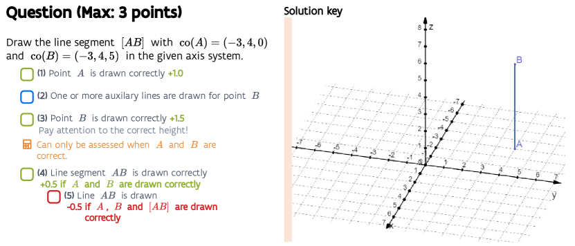
Figure 2: Example question of the math assessment tool

3.1.1 Context

The proposed $\kappa$ statistic was initially developed to measure the inter-rater reliability of multiple assessors assessing students with a new mathematics assessment method (Moons ., in preparation; Moons  Vandervieren,2022) for handwritten high-stakes exams called ‘checkbox grading.’ The method allows exam designers to preset a list of feedback items with partial scores for each question; so that assessors should just tick the items (= categories) relevant to a student’s answer. Hierarchical dependencies between items can be set, so items can be shown, disabled, or adapted whenever a previous item is ticked, implying that assessors must follow the preset point-by-point feedback items from top to bottom. This adaptive grading approach resembles a flow chart that automatically determines the grade. Moreover, checking the items that are relevant to a student’s answer might at the same time lead to several other envisioned benefits: (1) a deep insight into how the grade was obtained for both the student (feedback) as well as the exam designers and (2) a straightforward way to do correction work with multiple assessors where personal interpretations are avoided as much as possible.

An example of checkbox grading is given in Figure 2. With this drawing question, a student can gain a maximum score of 3 points. If point $A$ is drawn correctly (1 bullet), the student gains 1 point; the correct drawing of point $B$ (3 bullet) is worth 1.5 points. The 2 bullet does not change the score but shows assessors that the presence of auxiliary lines is perfectly fine. The last two feedback items, bullets 4 and 5, can only be selected if items 1 and 3 were selected. As the drawing of the line $AB$ implies the drawing of the line segment $AB$, the 5 bullet can only be selected if the 4 was. This is a clear example of hierarchical items (= categories).

During the project, one of the main research questions concerned the inter-rater reliability of this new assessment method under two conditions: blind versus visible grading. As the computer automatically calculated the grade associated with the selected checkboxes, it was possible to hide the grades and calculation from the assessors, which was the blind condition. In the visible condition, teachers could see how the items influenced the grade and how the total grade was calculated. From the literature on rubrics (Dawson, 2017), we know that judges often change the selection of criteria when the resulting grade does not align with their holistic appreciation of the work, which can affect the instrument’s reliability. As such, the research question was: ‘Does blind checkbox grading enhance inter-rater reliability compared to visible checkbox grading?’

The traditional measures for inter-rater reliability such as intraclass correlations fell short because these can only measure the agreement between asssessors on grades, while the method also provides feedback to students. Hence, it is not enough to agree on grades; the resulting feedback to the students must also be as equal as possible. Score agreement by no means guarantees agreement on feedback items, which is especially clear for feedback items not influencing the score (e.g., bullet 2 in the example). Other examples can be given as well: in Figure 2, 2.5 points can be obtained by solely drawing points $A$ and $B$ correctly (only bullets 1 and 3 apply, possibly bullet 2) or by drawing the line $AB$ correctly (all bullets apply, possibly bullet 2). Conversely, the inverse is true: agreement on feedback items implies score agreement.

Our proposed $\kappa$ statistic of subsection 2.2 does meet all requirements:

• It will assess the agreement of the raters in selecting multiple feedback items (= categories) for each student (= subjects)

• These items are hierarchical: the selectability of some items depends on the selection of other items

• Score agreement can naturally be measured by weighing the items according to their partial scores.

3.1.2 Example

We start with a worked-out example, in which our proposed $\kappa$ statistic is calculated step-by-step. We consider 3 assessors (i.e., the number of raters $J$ equals 3) assessing 6 students’ solutions (i.e., the number of subjects $I$ equals 6) on the question in Figure 2. The teachers classified every student’s solutions into the 5 items (i.e., the number of categories $C$ equals 5). The classifications by the three assessors of the six students’ answers can be found in Table 2. Although the example consists of a simple question, the tree assessors (raters) did sometimes select different items (categories) for the students’ solutions (subjects).

Table 2: Assessments by 3 teachers of 6 student’s answers on the example question

Teacher 1 Teacher 2 Teacher 3 S1 S2 S3 S4 S5 S6 S1 S2 S3 S4 S5 S6 S1 S2 S3 S4 S5 S6 (1) X X X X X X X X X X X X X X X X (2) X X X X X X X X X X X (3) X X X X X X X X X X (4) X X X X X X X X X (5) X X X Score 3 1 1 3 2.5 1 2.5 0 1 3 2.5 1 3 0 1 3 2.5 3

Specification of the weight vector $\mathbf{w}$

We start by specifying the weight vector $\mathbf{w}$. The associated scores for each item will evidently play a crucial role in defining these. However, note the second (blue) item does not influence the final grade on the question. If our weights would only represent the associated scores, then $w_{2}=0$; meaning that item 2 would not play any role in the calculation of our kappa-statistic, while the presence/absence of the item changes the feedback a student receives. Hence, instead of using the (absolute value) of the associated score to define the weights, we add the maximum absolute value of the associated scores over all items. This means that the weights will be defined based on $|\text{score}_{c}|+\max\{\left|\text{score}_{c}\right||\forall c\}$. To get weights between 0 and 1, we divide this sum by the doubled maximum associated score over all items:

$$w_{c}=\frac{|\text{score}_{c}|+\max\{\left|\text{score}_{c}\right||\forall c\}\}}{\max\{\left|\text{score}_{c}\right||\forall c\}\}}.$$ (32)

These weights have a nice interpretation: the minimum weight is always $0.5$, accounting for the (non-)selection of the item, everything between $0.5$ and $1$ depends on the (absolute value of) the associated score of the item. As such, items that do not influence the final score, will have weight of 0.5, while items with the maximum (absolute value of the) associated score will have weight 1. These weights do not sum to $1$, considering their interpretation is more intuitive this way. Based on formula (32), the calculated weights for the example are given in Table 3.

Table 3: Specification of the weight vector $\mathbf{w}$

Item		(1)	(2)	(3)	(4)	(5)
$|\text{score}_{c}|$	(associated score)	1	0	1.5	0.5	0.5
$\max\{\text{score}_{c}|\forall c\}\}s$	(selection)	1.5	1.5	1.5	1.5	1.5
Sum		2.5	1.5	3	2	2
Weight $w_{c}$		0.833	0.5	1	0.667	0.667

Determining the matrix of possible classifications $S$ and scale factors $\phi_{c}$ based on the hierarchical structure of the categories

We see that the first three items are all main categories: there are no conditions for (not) selecting them, so $s_{i1}=s_{i2}=s_{i3}=J=3$ for every student $i$. For a possible classification into item 4, item 1 and item 3 must be selected first; for example, student 6 has only the third teacher selecting these, so $s_{6,5}=1$. Item 5 can only be selected if item 4 was selected so $s_{i5}=x_{i4}$; for example, student 1 has 2 classifications for item 4 (teacher 1 & teacher 3), so $s_{1,5}=2$. Matrix $S$ can be found in Table 4.

The scale factors $\phi_{c}$ can be found by applying formula $\eqref{schaal}$: for each category $c$, loop over all subject $i$ and take the sum of the $s_{ic}$’s (sum up the columns of Table 4), and divide this sum by $IJ=6\cdot 3=18$.

Table 4: Determining the matrix of possible classifications $S$ and scale factors $\phi_{c}$

	$s_{i1}$	$s_{i2}$	$s_{i3}$	$s_{i4}$	$s_{i5}$
$s_{1c}$	3	3	3	3	2
$s_{2c}$	3	3	3	0	0
$s_{3c}$	3	3	3	0	0
$s_{4c}$	3	3	3	3	3
$s_{5c}$	3	3	3	3	3
$s_{6c}$	3	3	3	1	1
Sum	18	18	18	10	9
Scale factors	$\phi_{1}$	$\phi_{2}$	$\phi_{3}$	$\phi_{4}$	$\phi_{5}$
	1	1	1	0.556	0.5

Calculating $Po_{c}$ and $Pe_{c}$

We give the full calculation of $Po_{1}$ and $Pe_{2}$ in this paragraph. The other $Po_{c}$’s and $Pe_{c}$’s can be calculated in a similar way. The required $s_{i1}$ values were already calculated in the previous step, we still need to count how many times item 1 was selected for each student $i$ to get the $x_{i1}$ values; the results can be found in Table 5.

Table 5: Determining the $x_{i1}$’s and $s_{i1}$’s

Student	S1	S2	S3	S4	S5	S6
$x_{i1}$	3	1	3	3	3	3
$s_{i1}$	3	3	3	3	3	3

Next, we calculate $Po_{1}$ based on formula (27):

$$Po_{1} =\text{ $\frac{\left[3\cdot 2+0\cdot-1\right]+\left[1\cdot 0+2\cdot 1\right]+\left[3\cdot 2+0\cdot-1\right]+\left[3\cdot 2+0\cdot-1\right]+\left[3\cdot 2+0\cdot-1\right]+\left[3\cdot 2+0\cdot-1\right]}{3\cdot 2+3\cdot 2+3\cdot 2+3\cdot 2+3\cdot 2+3\cdot 2}$ }$$

$$=0.889,$$

For the computation of $Pe_{1}$, we use formula (28):

$$Pe_{1} =2\cdot\left(\frac{3+1+3+3+3+3}{3+3+3+3+3+3}\right)^{2}-2\cdot\left(\frac{3+1+3+3+3+3}{3+3+3+3+3+3}\right)+1$$

$$=0.802,$$

Although not necessary for the calculation of our proposed $\kappa$ statistic, it is possible to calculate the partial $\kappa_{c}$ to have an indication of the reliability of each item. For item 1, this becomes (see formula (10)):

$$\kappa_{1}=\frac{Po_{1}-Pe_{1}}{1-Pe_{1}}=\frac{0.889-0.802}{1-0.802}=0.438.$$

Although item 1 was selected for most students (only assessor 2 and 3 did not select it for student 2), we get a relatively low $\kappa_{1}$-value. How can this be explained? Item 1 was chosen for almost all students by almost all assessors, leading to a high agreement by chance $Pe_{1}(=0.802)$. This means that without even looking at a student’s solution, there is a high probability that an assessor selects item 1. The fact that student 2 has two non-classifications for item 1 while assessor 1 did select item 1 for this student leads, therefore, leads to a pretty severe penalisation in the partial kappa $\kappa_{1}$. This is a concrete example of the ‘prevalence paradox’ described in subsection 1.3.

The other $Po_{c}$’s and $Pe_{c}$’s can be calculated analogously. The result can be found in Table 6.

Table 6: $Po_{c}$, $Pe_{c}$, $Po-Pe$, $1-Pe$ and partial kappa $\kappa_{c}$ for every item (=category)

Items	(1)	(2)	(3)	(4)	(5)
$Po_{c}$	0.889	0.889	0.889	0.778	1.00
$Pe_{c}$	0.802	0.525	0.506	0.820	0.556
$Po_{c}-Pe_{c}$	0.086	0.364	0.383	-0.042	0.444
$1-Pe_{c}$	0.198	0.475	0.494	0.180	0.444
$\kappa_{c}$	0.438	0.766	0.775	-0.235	1.00

Calculation of the kappa-statistic

With the specification of weight vector $\mathbf{w}$, and the computation of the scale factors $\phi_{c}$, the ‘beyond-chance’ $Po_{c}-Pe_{c}$ and the ‘beyond-chance in case of perfectly agreeing raters’ $1-Pe_{c}$, we are ready to calculate the kappa-statistic for the hierarchical case (see formula (30)):

$$\kappa =\text{ $\frac{0.833\cdot 1\cdot 0.086+0.5\cdot 1\cdot 0.364+1\cdot 1\cdot 0.383+0.667\cdot 0.556\cdot(-0.042)+0.667\cdot 0.5\cdot 0.444}{0.833\cdot 1\cdot 0.198+0.5\cdot 1\cdot 0.475+1\cdot 1\cdot 0.494+0.667\cdot 0.556\cdot 0.180+0.667\cdot 0.5\cdot 0.444}$}$$

$$=0.692.$$

We get a relatively high $\kappa$-value, that would be labelled by the benchmark scale of Landis  Koch (1977) as ‘Substantial’ agreement.

Table 7: Multiple diagnostic formulations from 27 child psychiatric cases using DSM-III Axis I Broad Categories*

	Raters
Cases	1	2	3	4
1	9, 11	11, 9, 14	16, 9	11, 9
2	16	16, 14	12	14, 5
3	17	12	7, 8	13
4	16, 13	13, 16, 14	16
5	7	7, 12, 13	13
6	10	10	10
7	7, 16	13	16
8	1, 14	13	16, 13
9	5	20	13, 14
10	12, 13, 14	12, 14, 13	12, 11 14
11	13	18	16
12	5, 18	1, 5, 18	1
13	14, 13	14, 7	14, 16
14	11, 16	14, 11, 16	11, 13
15	10	3, 18	10, 11
16	14, 5	5, 16	14
17	12	12, 11	12
18	20	16	16
19	13	14	14
20	9, 14, 10	9, 11, 14	10, 9
21	12, 11	11, 14	11
22	17	12	12	12, 17, 15
23	16, 13	12	14	13
24	12	12	16	12
25	13	20	13	13
26	13	13, 16	13	16
27	10, 9	9, 10	9	9, 10

* 1. Organic mental disorders, 2. Substance use disorders, 3. Schizophrenic and paranoid disorders, 4. Schizoaffective disorders, 5. Affective disorder, 6. Psychoses not elsewhere classified, 7. Anxiety factitious, somatoform and dissociative disorders, 8. Pyschosexual disorder, 9. Mental retardation, 10. Pervasive developmental disorder, 11. Attention deficit disorders, 12. Conduct disorders, 13. Anxiety disorders of childhood or adolescence, 14. Other disorders of childhood or adolescence, speech and stereotyped movement disorders, disorders characteristic of late adolescence, 15. Eating disorders, 16. Reactive disorders not elsewhere classified, 17. Disorders of impulse control not elsewhere classified, 18. Sleep and other disorders, 19. Conditions not attributable to a mental disorder, 20. No diagnosis on Axis I.

3.1.3 Comparison with other methods

We also calculated this example through the other methods described in subsection 1.4. Averaging/pooling Cohen’s kappas is no possibility as we have more than two raters. The proportional overlap method is possible and returns $\kappa=0.602$. However, the method is based on some questionable premises in this context: (1) it assumes all items are equally weighted (so there is no correction for the associated scores), (2) it assumes all categories are always available to all raters (so the hierarchy of the items is ignored). Besides, the method fails to measure potential observed agreement for student 2 as $A_{22}=A_{23}=\emptyset$, no proportional overlaps can be calculated. Problems (1) and (2) also occur with the chance-corrected intraclass correlations that return a $\kappa$-value of $0.379$. The problem of failing to measure potential observed agreement for student 2 emerges in another guise: while the proportional overlap method leaves student 2 out of the calculation of $Po$, the chance-corrected intraclass correlations do include student 2 with an intraclass correlation coefficient of almost zero, pulling down the $Po$ value in an unacceptable way. While our proposed $\kappa$ statistic entails the philosophical premise that two raters not selecting category $c$ is equally valued in terms of agreement than two raters who do select category $c$; these examples show that the opposite - completely exclude agreement in non-selections - also can lead to unsatisfactory results. Finally, the calculation of chance-corrected rank correlations are not relevant in this context as raters do not make ordered classifications in checkbox grading.

3.2 Diagnosing psychiatric cases

We now revisit an example from Mezzich . (1981). It consists of a diagnostic exercise in which 30 child psychiatrist made independent diagnoses of 27 child psychiatric cases. Each psychiatrist rated 3 cases, and each case turned out to be rated by 3 or 4 psychiatrists upon completion of the study. Table 7 shows the 90 multiple diagnostic formulations. Each diagnostic formulation presented was composed of up to three from the twenty broad diagnostic categories taken from Axis I (clinical psychiatric syndromes) of the American Psychiatric Association’s Diagnostic and Statistical Manual of Mental Disorders (DSM-III). We are well aware that DSM-III is outdated (American Psychiatric Association, 2022), but the example remains excellent as it can be contrasted with the other measures in the literature.

We start with the calculation of our proposed $\kappa$ statistic. The example consists of 27 child psychiatric cases (i.e., the number of subjects $I$ equals 27), to be classified into $20$ broad diagnostic categories (i.e., the number of categories $C$ equals 20) with a varying number of raters, expressed in vector $\mathbf{j}$ with $j_{i}=3$ or $j_{i}=4$, depending on the case (see Table 8).

Table 8: Number of psychiatrists (= raters) for each case $i$ (= subject)

Cases	1	2	3	4	5	6	7	8	9	10	11	12	13	14	15	16	17	18	19	20	21	22	23	24	25	26	27
$j_{i}$	4	4	4	3	3	3	3	3	3	3	3	3	3	3	3	3	3	3	3	3	3	4	4	4	4	4	4

We assume all diagnostic categories are equally important and thus use unweighted categories ($w_{c}=1,\forall c$). Moreover, the diagnostic categories on Axis I have no hierarchy. Hence, we can use the formulas described in subsection 2.1. First, we calculate matrix $X$ by counting how many times a diagnostic category $c$ appeared for a subject $i$ (e.g., $x_{1,1}=0,x_{12,1}=2,x_{6,10}=3,\ldots$). Next, we combine the $x_{ic}$’s and the $j_{i}$’s to determine the $Po_{c}$’s (25) and the $Pe_{c}$’s (26). As an example, we calculate $Po_{1}$ and $Pe_{1}$:

$$Po_{1} =\text{ $\frac{9\left[2\mathop{\cdot}0^{2}\mathop{-}2\mathop{\cdot}4\mathop{\cdot}0\mathop{+}4^{2}\mathop{-}4\right]\mathop{+}16\left[2\mathop{\cdot}0^{2}\mathop{-}2\mathop{\cdot}3\mathop{\cdot}0\mathop{+}3^{2}\mathop{-}3\right]\mathop{+}1\left[2\mathop{\cdot}1^{2}\mathop{-}2\mathop{\cdot}3\mathop{\cdot}1\mathop{+}3^{2}\mathop{-}3\right]\mathop{+}1\left[2\mathop{\cdot}2^{2}\mathop{-}2\mathop{\cdot}3\mathop{\cdot}2\mathop{+}3^{2}\mathop{-}3\right]}{9\left[4(4\mathop{-}1)\right]\mathop{+}16\left[3(3\mathop{-}1)\right]\mathop{+}1\left[3(3\mathop{-}1)\right]\mathop{+}1\left[3(3\mathop{-}1)\right]}$ }$$

$$=0.963$$

$$Pe_{1} =2\left(\frac{9\mathop{\cdot}0+16\mathop{\cdot}0+1\mathop{\cdot}1+1\mathop{\cdot}2}{9\mathop{\cdot}4+16\mathop{\cdot}3+1\mathop{\cdot}3+1\mathop{\cdot}3}\right)^{2}+2\left(\frac{9\mathop{\cdot}0+16\mathop{\cdot}0+1\mathop{\cdot}1+1\mathop{\cdot}2}{9\mathop{\cdot}4+16\mathop{\cdot}3+1\mathop{\cdot}3+1\mathop{\cdot}3}\right)+1$$

$$=0.936.$$

The other calculations can be found in Table 9.

Table 9: $Po_{c}$, $Pe_{c}$, $Po-Pe$, $1-Pe$ and partial kappa $\kappa_{c}$ for every diagnostic category

Diagnostic category 1 2 3 4 5 6 7 8 9 10 $Po_{c}$ 0.963 1.000 0.981 1.000 0.917 1.000 0.917 0.972 1.000 0.935 $Pe_{c}$ 0.936 1.000 0.978 1.000 0.876 1.000 0.895 0.978 0.785 0.802 $Po_{c}-Pe_{c}$ 0.027 0.000 0.003 0.000 0.041 0.000 0.022 -0.006 0.215 0.133 $1-Pe_{c}$ 0.064 0.000 0.022 0.000 0.124 0.000 0.105 0.022 0.215 0.198 $\kappa_{c}$ 0.425 NaN 0.157 NaN 0.330 NaN 0.206 -0.264 1.000 0.672 Diagnostic category 11 12 13 14 15 16 17 18 19 20 $Po_{c}$ 0.898 0.824 0.694 0.759 0.972 0.713 0.935 0.944 1.000 0.935 $Pe_{c}$ 0.753 0.694 0.620 0.642 0.978 0.654 0.936 0.915 1.000 0.936 $Po_{c}-Pe_{c}$ 0.145 0.130 0.075 0.117 -0.006 0.059 0.000 0.029 0.000 0.000 $1-Pe_{c}$ 0.247 0.306 0.380 0.358 0.022 0.346 0.064 0.085 0.000 0.064 $\kappa_{c}$ 0.588 0.426 0.197 0.327 -0.264 0.170 -0.006 0.346 NaN -0.006

Note that $\kappa_{2},\kappa_{4},\kappa_{6}$ and $\kappa_{19}$ equal NaN, due to a division by zero. Such division by zero will always happen if no rater chooses a category. As $Po_{c}=Pe_{c}=1$ in those categories and thus $Po-Pe=1-Pe=0$, these unchosen categories do not play any role in the calculation of the proposed $\kappa$ statistic. Hence, the $\kappa$ statistic is independent of unused alternative categories, meaning it can not be inflated by adding unchosen categories; we get from formula (18):

$$\kappa=\frac{\displaystyle\sum_{c}(Po_{c}-Pe_{c})}{\displaystyle\sum_{c}(1-Pe_{c})}=0.375.$$

We get a relatively low kappa-value, which should not come unexpected: Table 7 shows that the various psychiatrists diverge rather vehemently in their diagnoses. The proposed $\kappa$ statistic yields a much lower value than the proportional overlap method ($\kappa=0.27$), but is almost equal to the chance-corrected intraclass correlation method ($\kappa=0.35$) and the rank correlation method ($\kappa=0.34$).

4 Further research

The story of the proposed $\kappa$ statistic is not finished by publishing this preprint. First, the publication of an R package is envisioned containing ready-to-use functions to calculate all described measures. Such a package would allow researchers without an overly statistical background to use the measure in their research and can greatly facilitate the adoption of the proposed measure.

In addition, more can be told about the proposed measure. Based on De Vries . (2008), we envision publishing the simulation study to show that our proposed kappa statistic exhibits smaller root-mean-square errors than taking a weighted average of Fleiss’ kappas. Moreover, the large-sample variance of the proposed $\kappa$ statistic still needs to be determined. An expression for the variance would enable statistical inference using the measure without bootstrapping. It especially paves the way for performing robust power analysis: researchers wishing to set up an experiment in which raters classify subjects into one-or-more categories would be able to calculate in advance the number of raters and subjects required to reach a certain confidence level. Finding the large-sample variance of our proposed $\kappa$ statistic is by no means an easy quest: it took the scientific community 50 years to develop a general expression for the Fleiss’ kappa! Indeed, it was Gwet (2021) who finally came up with a correct formula for the variance of the Fleiss’ kappa. The variance described in Fleiss (1971) is simply wrong; the standard error of Fleiss . (1979) is valid only under the assumption of no agreement among raters; as such, it can only be used to test the hypothesis of zero agreement among the raters. Unfortunately, as many statistical software programs provide the standard error of Fleiss . (1979) along with the calculation of Fleiss’ kappa, it is immensely misused for all kinds of statistical inference. Let us avoid making the same mistakes when searching a large-sample variance of our proposed measure that presumably entails a generalisation of the formula found by Gwet (2021).

To conclude: now that we have established the idea of the proposed $\kappa$ statistic, the same idea may be suitable to create other long-needed measures. For example, the literature on rubrics (Dawson, 2017) lacks a unified way to compare the inter-rater reliability of two rubrics assessing the same phenomenon (e.g. book reviews of students, PhD proposals). Should such a measure exists, it would be possible to compare the impact of including/excluding specific criteria. Such a measure can possibly be constructed by the calculation of the $Po$ and $Pe$ of the Fleiss kappa (or the Krippendorff’s alpha, see Gwet (2012)) for groups of criteria assessing the same aspect and weighting them according to the maximum score of the aspect.

5 Conclusion

This paper has presented a generalisation of Fleiss’ kappa, allowing raters to select multiple categories for each subject. Categories can be weighted according to their importance in the research context, and the measure can account for possible hierarchical dependencies between the categories. A crucial assumption of the proposed $\kappa$ statistic is that two raters selecting a specific category for a given subject count equally in agreement as two raters not selecting the category. Other methods, like proportional overlap, chance-corrected intraclass correlations and chance-corrected rank correlations, do not make this assumption; instead, they ignore the agreement in the non-selection of categories. We have shown that this ignorance can give unexpected and unwanted results depending on the research context. By introducing this generalisation of Fleiss’ kappa and comparing and contrasting it to the existing comparable methods, we hope to inspire further researchers in need of a chance-corrected inter-rater reliability measure that allows measuring the agreement among several raters classifying subjects into one-or-more (hierarchical) nominal categories.

Funding

This research is funded by a doctoral fellowship (1S95920N) granted to Filip Moons by FWO, the Research Foundation of Flanders (Belgium).

References

- American Psychiatric Association (\APACyear2022) \APACinsertmetastarAssociation2022{APACrefauthors}American Psychiatric Association. \APACrefYear2022. \APACrefbtitleDiagnostic and Statistical Manual of Mental Disorders Diagnostic and statistical manual of mental disorders. \APACaddressPublisherAmerican Psychiatric Association Publishing. {APACrefDOI} 10.1176/appi.books.9780890425787 \PrintBackRefs\CurrentBib
- Bennett \BOthers. (\APACyear1954) \APACinsertmetastarBENNETT1954{APACrefauthors}Bennett, E., Alpert, R.\BCBL \BBA Goldstein, A. \APACrefYearMonthDay1954. \BBOQ\APACrefatitleCommunications Through Limited-Response Questioning* Communications Through Limited-Response Questioning*.\BBCQ \APACjournalVolNumPagesPublic Opinion Quarterly183303,308. {APACrefDOI} 10.1086/266520 \PrintBackRefs\CurrentBib
- Cohen (\APACyear1960) \APACinsertmetastarcohen1{APACrefauthors}Cohen, J. \APACrefYearMonthDay1960. \BBOQ\APACrefatitleA Coefficient of Agreement for Nominal Scales A coefficient of agreement for nominal scales.\BBCQ \APACjournalVolNumPagesEducational and Psychological Measurement20137-46. {APACrefDOI} 10.1177/001316446002000104 \PrintBackRefs\CurrentBib
- Conger (\APACyear1980) \APACinsertmetastarConger1980{APACrefauthors}Conger, A\BPBIJ. \APACrefYearMonthDay1980sep. \BBOQ\APACrefatitleIntegration and generalization of kappas for multiple raters. Integration and generalization of kappas for multiple raters.\BBCQ \APACjournalVolNumPagesPsychological Bulletin882322–328. {APACrefDOI} 10.1037/0033-2909.88.2.322 \PrintBackRefs\CurrentBib
- Dawson (\APACyear2017) \APACinsertmetastardawson{APACrefauthors}Dawson, P. \APACrefYearMonthDay2017. \BBOQ\APACrefatitleAssessment rubrics: towards clearer and more replicable design, research and practice Assessment rubrics: towards clearer and more replicable design, research and practice.\BBCQ \APACjournalVolNumPagesAssessment & Evaluation in Higher Education423347-360. {APACrefDOI} 10.1080/02602938.2015.1111294 \PrintBackRefs\CurrentBib
- De Vries \BOthers. (\APACyear2008) \APACinsertmetastarVries2008{APACrefauthors}De Vries, H., Elliott, M\BPBIN., Kanouse, D\BPBIE.\BCBL \BBA Teleki, S\BPBIS. \APACrefYearMonthDay2008mar. \BBOQ\APACrefatitleUsing Pooled Kappa to Summarize Interrater Agreement across Many Items Using pooled kappa to summarize interrater agreement across many items.\BBCQ \APACjournalVolNumPagesField Methods203272–282. {APACrefDOI} 10.1177/1525822x08317166 \PrintBackRefs\CurrentBib
- Feinstein \BBA Cicchetti (\APACyear1990) \APACinsertmetastarFEINSTEIN1990543{APACrefauthors}Feinstein, A\BPBIR.\BCBT \BBA Cicchetti, D\BPBIV. \APACrefYearMonthDay1990. \BBOQ\APACrefatitleHigh agreement but low Kappa: I. the problems of two paradoxes High agreement but low kappa: I. the problems of two paradoxes.\BBCQ \APACjournalVolNumPagesJournal of Clinical Epidemiology436543-549. {APACrefDOI} 10.1016/0895-4356(90)90158-L \PrintBackRefs\CurrentBib
- Fleiss (\APACyear1971) \APACinsertmetastarfleiss1971measuring{APACrefauthors}Fleiss, J\BPBIL. \APACrefYearMonthDay1971. \BBOQ\APACrefatitleMeasuring nominal scale agreement among many raters. Measuring nominal scale agreement among many raters.\BBCQ \APACjournalVolNumPagesPsychological bulletin765378. {APACrefDOI} 10.1037/h0031619 \PrintBackRefs\CurrentBib
- Fleiss \BOthers. (\APACyear1979) \APACinsertmetastarFleiss1979{APACrefauthors}Fleiss, J\BPBIL., Nee, J\BPBIC.\BCBL \BBA Landis, J\BPBIR. \APACrefYearMonthDay1979sep. \BBOQ\APACrefatitleLarge sample variance of kappa in the case of different sets of raters. Large sample variance of kappa in the case of different sets of raters.\BBCQ \APACjournalVolNumPagesPsychological Bulletin865974–977. {APACrefDOI} 10.1037/0033-2909.86.5.974 \PrintBackRefs\CurrentBib
- Gwet (\APACyear2008) \APACinsertmetastarGwet2008{APACrefauthors}Gwet, K\BPBIL. \APACrefYearMonthDay2008. \BBOQ\APACrefatitleComputing inter-rater reliability and its variance in the presence of high agreement. Computing inter-rater reliability and its variance in the presence of high agreement.\BBCQ \APACjournalVolNumPagesThe British journal of mathematical and statistical psychology6129-48. {APACrefDOI} 10.1348/000711006X126600 \PrintBackRefs\CurrentBib
- Gwet (\APACyear2012) \APACinsertmetastargwet{APACrefauthors}Gwet, K\BPBIL. \APACrefYear2012. \APACrefbtitleHandbook of inter-rater reliability: The definitive guide to measuring the extent of agreement among raters Handbook of inter-rater reliability: The definitive guide to measuring the extent of agreement among raters. \APACaddressPublisherAdvanced Analytics, LLC. \PrintBackRefs\CurrentBib
- Gwet (\APACyear2021) \APACinsertmetastardoi:10.1177/0013164420973080{APACrefauthors}Gwet, K\BPBIL. \APACrefYearMonthDay2021. \BBOQ\APACrefatitleLarge-Sample Variance of Fleiss Generalized Kappa Large-sample variance of fleiss generalized kappa.\BBCQ \APACjournalVolNumPagesEducational and Psychological Measurement814781-790. {APACrefDOI} 10.1177/0013164420973080 \PrintBackRefs\CurrentBib
- Kraemer (\APACyear1980) \APACinsertmetastarkraemer_extend{APACrefauthors}Kraemer, H\BPBIC. \APACrefYearMonthDay1980. \BBOQ\APACrefatitleExtension of the Kappa Coefficient Extension of the kappa coefficient.\BBCQ \APACjournalVolNumPagesBiometrics362207–216. {APACrefDOI} 10.2307/2529972 \PrintBackRefs\CurrentBib
- Kraemer \BOthers. (\APACyear2002) \APACinsertmetastarKraemer2002{APACrefauthors}Kraemer, H\BPBIC., Periyakoil, V\BPBIS.\BCBL \BBA Noda, A. \APACrefYearMonthDay2002. \BBOQ\APACrefatitleKappa coefficients in medical research Kappa coefficients in medical research.\BBCQ \APACjournalVolNumPagesStatistics in Medicine21142109–2129. {APACrefDOI} 10.1002/sim.1180 \PrintBackRefs\CurrentBib
- Landis \BBA Koch (\APACyear1977) \APACinsertmetastarLandis1977{APACrefauthors}Landis, J\BPBIR.\BCBT \BBA Koch, G\BPBIG. \APACrefYearMonthDay1977. \BBOQ\APACrefatitleThe Measurement of Observer Agreement for Categorical Data The measurement of observer agreement for categorical data.\BBCQ \APACjournalVolNumPagesBiometrics331159. {APACrefDOI} 10.2307/2529310 \PrintBackRefs\CurrentBib
- Little (\APACyear1988) \APACinsertmetastarLittle{APACrefauthors}Little, R\BPBIJ\BPBIA. \APACrefYearMonthDay1988. \BBOQ\APACrefatitleA Test of Missing Completely at Random for Multivariate Data with Missing Values A test of missing completely at random for multivariate data with missing values.\BBCQ \APACjournalVolNumPagesJournal of the American Statistical Association834041198-1202. {APACrefDOI} 10.1080/01621459.1988.10478722 \PrintBackRefs\CurrentBib
- Mezzich \BOthers. (\APACyear1981) \APACinsertmetastarMEZZICH198129{APACrefauthors}Mezzich, J\BPBIE., Kraemer, H\BPBIC., Worthington, D\BPBIR.\BCBL \BBA Coffman, G\BPBIA. \APACrefYearMonthDay1981. \BBOQ\APACrefatitleAssessment of agreement among several raters formulating multiple diagnoses Assessment of agreement among several raters formulating multiple diagnoses.\BBCQ \APACjournalVolNumPagesJournal of Psychiatric Research16129-39. {APACrefDOI} 10.1016/0022-3956(81)90011-X \PrintBackRefs\CurrentBib
- Moons \BOthers. (\APACyearin preparation) \APACinsertmetastarmoons1{APACrefauthors}Moons, F., Colpaert, J.\BCBL \BBA Vandervieren, E. \APACrefYearMonthDayin preparation. \APACrefbtitleCheckbox grading: a semi-automated way assess and give atomic feedback to handwritten mathematics exams with multiple teachers? A study into time investment, reliability and teachers’ use and perceivement. Checkbox grading: a semi-automated way assess and give atomic feedback to handwritten mathematics exams with multiple teachers? a study into time investment, reliability and teachers’ use and perceivement. \APACrefnoteWill be send to Educational Studies in Mathematics \PrintBackRefs\CurrentBib
- Moons \BBA Vandervieren (\APACyear2022) \APACinsertmetastarmoons:hal-03753446{APACrefauthors}Moons, F.\BCBT \BBA Vandervieren, E. \APACrefYearMonthDay2022. \BBOQ\APACrefatitleHandwritten math exams with multiple assessors: researching the added value of semi-automated assessment with atomic feedback Handwritten math exams with multiple assessors: researching the added value of semi-automated assessment with atomic feedback.\BBCQ \BIn \APACrefbtitleTwelfth Congress of the European Society for Research in Mathematics Education (CERME12) Twelfth Congress of the European Society for Research in Mathematics Education (CERME12) (\BVOL TWG21). \APACaddressPublisherBozen-Bolzano, Italy. {APACrefURL} https://hal.science/hal-03753446 \PrintBackRefs\CurrentBib
- NVivo (\APACyear2022) \APACinsertmetastarnvivo{APACrefauthors}NVivo. \APACrefYearMonthDay2022. \APACrefbtitleRun a Coding Comparison query Run a coding comparison query \APACbVolEdTR\BTR. \APACaddressInstitutionNVivo 11. {APACrefURL} https://help-nv11.qsrinternational.com/desktop/procedures/run_a_coding_comparison_query.htm \PrintBackRefs\CurrentBib
- Osgood (\APACyear1959) \APACinsertmetastarOsgood1959{APACrefauthors}Osgood, C\BPBIE. \APACrefYearMonthDay1959. \BBOQ\APACrefatitleThe Representational Model and Relevant Research Methods The representational model and relevant research methods.\BBCQ \BIn I. Pool (\BED), \APACrefbtitleTrends in content analysis Trends in content analysis (\BPGS 33,38). \APACaddressPublisherUrbana: University of Illinois Press. \PrintBackRefs\CurrentBib
- Vanacore \BBA Pellegrino (\APACyear2022) \APACinsertmetastarsubjective{APACrefauthors}Vanacore, A.\BCBT \BBA Pellegrino, M\BPBIS. \APACrefYearMonthDay2022. \BBOQ\APACrefatitleBenchmarking procedures for characterizing the extent of rater agreement: a comparative study Benchmarking procedures for characterizing the extent of rater agreement: a comparative study.\BBCQ \APACjournalVolNumPagesQuality and Reliability Engineering International3831404-1415. {APACrefDOI} 10.1002/qre.2982 \PrintBackRefs\CurrentBib
- Warrens (\APACyear2010) \APACinsertmetastarWarrens2010{APACrefauthors}Warrens, M\BPBIJ. \APACrefYearMonthDay2010oct. \BBOQ\APACrefatitleA Formal Proof of a Paradox Associated with Cohen’s Kappa A formal proof of a paradox associated with cohen’s kappa.\BBCQ \APACjournalVolNumPagesJournal of Classification273322–332. {APACrefDOI} 10.1007/s00357-010-9060-x \PrintBackRefs\CurrentBib