Prethermalization in coupled one-dimensional quantum gases

Maciej Łebek^1$\star$, Miłosz Panfil¹ and Robert M. Konik²

Abstract

We consider the problem of the development of steady states in one-dimensional Bose gas tubes that are weakly coupled to one another through a density-density interaction. We analyze this development through a Boltzmann collision integral approach. We argue that when the leading order of the collision integral, where single particle-hole excitations are created in individual gases, is dominant, the state of the gas evolves first to a non-thermal fixed point, i.e. a prethermalization plateau. This order is dominant when a pair of tubes are inequivalent with, say, different temperatures or different effective interaction parameters, $\gamma$. We characterize this non-thermal prethermalization plateau, constructing both the quasi-conserved quantities that control the existence of this plateau as well as the associated generalized Gibbs ensemble.

 

Contents

1. 1 Introduction
2. 2 Summary of the Lieb-Liniger model
3. 3 Coupled Lieb-Liniger gases
   1. 3.1 (n,m) ph processes
   2. 3.2 Stationary states
   3. 3.3 Conservation laws
4. 4 (1,1) dynamics in the small momentum limit
   1. 4.1 Stationary states
      1. 4.1.1 Tonks-Girardeau limit in both tubes
      2. 4.1.2 Perturbative solution in both tubes
   2. 4.2 Conserved charges
   3. 4.3 Numerical construction of conserved charges
5. 5 Generalized Gibbs Ensemble for (1,1) dynamics in the small momentum limit
6. 6 Numerical results
   1. 6.1 Bragg-split states
   2. 6.2 Two different thermal states
7. 7 Summary and Conclusion
8. A Scaling of the collision integral in the small momentum limit
9. B Absence of non-thermal stationary states beyond the small momentum limit
10. C Perturbative solution of the stationary state equation

 

1 Introduction

How to understand the dynamics of a quantum system after the injection of energy is a paramount problem of modern many-body physics [1, 2, 3]. The injection of energy typically leads a system to arrive at a new steady state that is thermal in nature. The process by which this occurs in closed quantum systems is governed by the eigenstate thermalization hypothesis (ETH) [4, 5, 6, 7, 8]. This hypothesis asserts that quantum eigenstates of similar energy behave similarly with respect to all local observables, at least in the thermodynamic limit. However this hypothesis is not inviolate and there are models where ETH does not hold. One such class of ETH violating systems that has been extensively studied in the past few years support what are known as quantum scar states [9, 10, 11, 12]. Quantum scar states have expectation values relative to some local observable that differs significantly from most other system eigenstates at the same energy. When a system is then in a scar state, it will experience atypical time dynamics relative to that observable and will not thermalize in the sense of ETH.

Another class of ETH violating systems are integrable models. Integrable models are characterized by an infinite set of conservation laws. The presence of these conservation laws means that their steady states are characterized by more complicated thermodynamic ensembles than Gibbs that take into account the presence of conserved charges beyond energy [13, 8] Integrable models are ubiquitous in one-spatial dimension. Such models describe the dynamics of cold atomic Bose gases via the Lieb-Liniger model [14, 15], XXZ spin chains via the Heisenberg spin model [16], and itinerant interacting electron physics via the Hubbard model [17, 18] to name but a few.

Integrable models are to a certain degree platonic ideals. They only exist approximately in nature. Experimental realizations of one-dimensional Bose gases modelled by a Lieb-Linger (LL) model involve arrays of one-dimensional tubes of the gas which see both intra- and intertube interactions beyond the interactions present in the LL Hamiltonian [19, 20, 21]. Similarly, quantum material realizations of one-dimensional spin chains are always in fact one-dimensional atomic chains embedded in a three dimensional matrix with interchain interactions, perhaps small but nonetheless, present [22, 23]. Finally, also material realizations of low-dimensional Hubbard models typically require the reduction of complicated multi-orbital physics down to effective one-band models [24, 25, 26, 27].

The interactions that go beyond those present in integrable Hamiltonians will almost always break integrability. While an integrable model will not thermalize, a quasi-integrable model will (apart from cases when quantum scars are present). However it then becomes a question of timescales. Rather than a non-thermal steady state persisting for all time, it instead picks up a finite, but perhaps long, lifetime. This persistent non-thermal steady state is known as a prethermalization plateau [28, 29]. This prethermalization plateau is characterized by conserved quantities other than energy. However these conserved quantities are not necessarily the same as in the parent, unperturbed, integrable model.

It is the aim of this paper to present a scenario relevant to experiments in one-dimensional cold atomic Bose gases where long-live prethermalization plateaus occur. In typical realizations of one-dimensional Bose gases, the atoms in the gas are placed in an laser-induced array of quasi-one-dimensional transversal confining potentials, i.e. the gas forms of matrix of tubes [19, 20, 21]. The atoms in each tube are typically confined to the lowest transverse level of the tube but are free to move laterally along the tube. However the gas in each tube is not entirely independent of its neighbours in the array. Typically intertube density-density interactions are present. Such interactions in gases with dipolar couplings are tunable and can even made to be of the same order as intratube interactions [19].

In Ref. [30] a framework for analyzing the thermalizing effects of intertube interactions was developed in the form of a Boltzmann collision integral. In Ref. [30], the tubes of gas were considered to be identical. A key feature of this work was then that the thermalizing interactions involve processes of the simultaneous creation of three particle-hole pairs in any two tubes: one pair in one tube and two pairs in a second tube, so-called (2,1) or (1,2) processes. Processes involving the production of a single pair in two identical tubes, (1,1) processes, led to no change in the state of the tubes, a simple consequence of energy-momentum conservation.

If however the two tubes are inequivalent, either by virtue of having a different density of atoms or a different effective interaction parameter, (1,1) processes are dominant at shorter time scales and do lead to an evolution in the state of the gas in the tube. However here the end point of this evolution is athermal. Because we cannot ignore (1,2)/(2,1) processes, this athermal state arrived at by the creation of single particle-hole pairs is temporary – it is in fact a prethermalization plateau. Nonetheless it is long-lived if the intertube interactions, which set the scale of the evolution, are weak. It is the aim of this paper to describe in detail the resulting athermal state coming from tube heterogeneity.

The athermality of the state resulting from (1,1) processes is governed by an emergent set of conserved charges. These charges are related to those present in the uncoupled tubes: we show that it is possible to construct approximations to the new conserved charges governing the prethermalization plateau as linear combinations of the conserved charges of the uncoupled Lieb-Linger models. We construct both the emergent charges as well as characterizing the associated non-Gibbsian ensemble governing the prethermalization plateau’s steady state.

While the focus of this analysis takes place in the context of cold atomic systems, the analysis has elements of universality. A very similar set of considerations, for example, would apply to thermalizing $S_{z}S_{z}$ interchain interactions in spin chain materials. The universality arises because in the thermodynamic limit the matrix elements governing the creation of particle hole pairs (and their spin chain equivalents) have the same low energy form [31, 32].

The paper is organized as follows. In Section 2 we outline the basics of the Lieb-Liniger model including how to describe its thermodynamic states and its conserved quantities. In the next section, Section 3, we present the Boltzmann collision framework by which we analyze the dynamics of two tubes of gas due to intertube interactions. As part of this we present a general analysis of what constitutes a steady state in this framework and what are its conservation laws. We do this in complete generality considering all orders of particle-hole creation (i.e. (n,m)) processes. As part of this, we show that only energy, momentum, and particle number survive as conserved quantities and the resulting steady state is thermal. But in the next two sections, Section 4 and 5, we perform this same analysis but only considering (1,1) processes. Here we show that with only (1,1) processes taken into account, new non-trivial conservation laws beyond energy, momentum, and particle number arise and that these laws lead to athermal steady states. We show that it is possible to describe the non-Gibbsian ensemble (i.e. the generalized Gibbs ensemble) characterizing the steady state. In Section 6 we then turn to concrete numerical examples of the dynamics where only (1,1) processes are operative. Finally, in Section 8, we provide a summary and concluding remarks.

2 Summary of the Lieb-Liniger model

We start with reviewing the relevant aspects of the Lieb-Liniger (LL) model [14, 15], which corresponds to a single gas tube. The LL model describes $N$ bosons on a ring with length $L$, interacting with a repulsive contact potential. The Hamiltonian of the system reads

$$\hat{H}_{LL}=\int_{0}^{L}dx\Big{(}-\hat{\psi}^{\dagger}(x)\partial_{x}^{2}\hat{\psi}(x)+c\hat{\psi}^{\dagger}(x)\hat{\psi}^{\dagger}(x)\hat{\psi}(x)\hat{\psi}(x)\Big{)}$$ (1)

where $c\geq 0$ is the coupling constant and $\hat{\psi}(x)$ is the canonical bosonic field operator. The model is exactly solvable with the standard Bethe ansatz technique [33, 34, 35]. Eigenstates of (1) are parametrized by $N$ real numbers, called quasimomenta, which are determined from the Bethe equations. In the thermodynamic limit $N,L\to\infty$ with $N/L={\rm const}$, the system is parametrized by the density of particles, $\rho_{p}(\lambda)$, and the total density of states, $\rho_{t}(\lambda)$, with $\lambda$ the quasi-momentum or rapidity. These functions are related through the following integral equation [36],

$$\rho_{t}(\lambda)=\frac{1}{2\pi}+\int d\lambda^{\prime}\,T(\lambda-\lambda^{\prime})\rho_{p}(\lambda^{\prime}),$$ (2)

with the kernel given by function, $T(\lambda)$:

$$T(\lambda)=\frac{c}{\pi}\frac{1}{c^{2}+\lambda^{2}}.$$ (3)

In addition to $\rho_{t}$ and $\rho_{p}$, we define the density of holes, $\rho_{h}$, as

$$\rho_{h}(\lambda)=\rho_{t}(\lambda)-\rho_{p}(\lambda).$$ (4)

It is sometimes convenient to express thermodynamic quantities in terms of $\rho_{h}$ rather than $\rho_{p}$.

The LL model is integrable and so is characterized by an infinite number of conserved charges, $\hat{I}_{n}$, that commute with the Hamiltonian (1) and have the property

$$[\hat{I}_{n},\hat{I}_{m}]=0,\qquad n,m=0,1,2,\ldots$$ (5)

There are multiple bases of these charges, both ultra-local [37] and semi-local [38, 39, 40]. In this work we will focus on the ultra-local representation despite their less than stellar behaviour in the UV [41]. Expectation values of the ultra-local conserved charges on thermodynamic states are functionals of the distribution, $\rho_{p}(\lambda)$, and take the particularly simple form

$$\langle\hat{I}_{n}\rangle=L\int d\lambda\,\rho_{p}(\lambda)\lambda^{n}.$$ (6)

The first operators in the sequence, $\hat{I}_{n}$, correspond to particle number, total momentum and total energy, $n=0,1,2$, respectively:

$$N=L\int d\lambda\rho_{p}(\lambda),\quad P=L\int d\lambda\,\lambda\rho_{p}(\lambda),\quad E=L\int d\lambda\,\lambda^{2}\rho_{p}(\lambda).$$ (7)

The presence of conserved charges $n>2$ beyond these basic three means that the model can support non-thermal states. We will argue that even when integrability is broken by intertube interactions that remnant quasi-conserved quantities remain and lead to the formation of prethermalization plateaus.

We now turn to characterizing the thermodynamics and elementary excitations of the LL model. The entropy of a thermodynamic state of the gas is given by the Yang-Yang formula [36]

$$S=L\int d\lambda\Big{[}\big{(}\rho_{p}(\lambda)+\rho_{h}(\lambda)\big{)}\log\big{(}\rho_{p}(\lambda)+\rho_{h}(\lambda)\big{)}-\rho_{p}(\lambda)\log\rho_{p}(\lambda)-\rho_{h}(\lambda)\log\rho_{h}(\lambda)\Big{]}.$$ (8)

To describe the dynamics in the system we also need information about its elementary excitations. The coupling between the tubes that we consider, conserves number of particles in each tubes. Therefore the relevant excitations takes form of particle-hole (ph) excitations in the system  [15, 42]. The excitations are labelled by two quasimomenta $p$ and $h$. The momentum carried by an excitation is $k=k(p)-k(h)$ and the corresponding energy is $\omega=\omega(p)-\omega(h)$. Here, the functions $k(p)$ and $\omega(p)$ are the so-called dressed momentum and energy. These are state-dependent functions and read

$$k(\lambda)=\lambda-\int d\mu\,n(\mu)F(\mu|\lambda),$$ (9a)

$$\omega(\lambda)=\lambda^{2}-2\int d\mu\,\mu n(\mu)F(\mu|\lambda),$$ (9b)

where $n(\lambda)=\rho_{p}(\lambda)/\rho_{t}(\lambda)$ is the occupation function and $F(\mu|\lambda)$ is the backflow function [42] satisfying the following integral equation,

$$F(\lambda|\mu)=\frac{\theta(\lambda-\mu)}{2\pi}+\int d\lambda^{\prime}T(\lambda-\lambda^{\prime})n(\lambda^{\prime})F(\lambda^{\prime}|\mu),$$ (10)

with $\theta(\lambda)=2\arctan(\lambda/c)$.

For later use, we introduce notation for two dressing operations, following the notation of [43]. The first one, denoted ${\rm Dr}$, is defined as

$$f_{Dr}(\lambda)=f(\lambda)-\int{\rm d}\mu\,n(\mu)F(\mu|\lambda)n(\mu)f^{\prime}(\mu).$$ (11)

Therefore $k(\lambda)=(\lambda)_{Dr}$ and $\omega(\lambda)=(\lambda^{2})_{Dr}$. The second one, denoted ${\rm dr}$, is defined as

$$f_{dr}(\lambda)=f(\lambda)+\int{\rm d}\mu\,T(\mu,\lambda)n(\mu)f_{dr}(\mu).$$ (12)

The two dressing operations are related however through

$$(f_{\rm Dr})^{\prime}=(f^{\prime})_{\rm dr}.$$ (13)

3 Coupled Lieb-Liniger gases

In this section, we present a framework to study the dynamics of two coupled LL gases. The system is governed by the following Hamiltonian,

$$\hat{H}=\hat{H}_{LL,1}+\hat{H}_{LL,2}+\int dx_{1}dx_{2}A(x_{1}-x_{2})\hat{\rho}_{1}(x_{1})\hat{\rho}_{2}(x_{2}).$$ (14)

The Hamiltonians $\hat{H}_{LL,i}$ describe LL gases with couplings $c_{i}$. The two gases are coupled by a long-range interaction potential $A(x_{1}-x_{2})$. By $\hat{\rho}_{i}(x)=\hat{\psi}^{\dagger}_{i}(x)\hat{\psi}_{i}(x)$, we denote the density operator in the $i$-th gas. The density-density interaction term $\delta\hat{H}$ breaks the integrability of the system $\hat{H}=\hat{H}_{\text{int}}+\delta\hat{H}$, where $\hat{H}_{\text{int}}=\hat{H}_{LL,1}+\hat{H}_{LL,2}$ is integrable. To describe its consequences on the gases’ dynamics, we turn to an effective theory of relaxation developed in [44, 30]. Specifically in [30] the problem of the thermalization of two equivalent gases initialized in a non-thermal state was analyzed in quantitative detail. On the level of Fermi’s golden rule approximation, the dynamics may be formulated in terms of Boltzmann-like equations governing the evolution of the rapidity distributions:

$$\begin{split}&\partial_{t}\rho_{p,1}(\lambda)=\tau^{-1}Q[\rho_{p,1},\rho_{p,2}](\lambda),\\ &\partial_{t}\rho_{p,2}(\lambda)=\tau^{-1}Q[\rho_{p,2},\rho_{p,1}](\lambda),\end{split}$$ (15)

where $\tau$ is the characteristic time scale for the evolution and $Q[\rho_{p,1};\rho_{p,2},\lambda]$ is the dressed scattering integral defined through

$$\begin{split}Q[\rho_{p,1},\rho_{p,2}]=\mathbb{F}_{1}\cdot Q_{0}[\rho_{\rm p,1},\rho_{\rm p,2}],\\ Q[\rho_{\rm p,2},\rho_{\rm p,1}]=\mathbb{F}_{2}\cdot Q_{0}[\rho_{\rm p,2},\rho_{\rm p,1}].\end{split}$$ (16)

Here $\mathbb{F}_{i}(\lambda,\mu)$ is defined by

$$\mathbb{F}_{i}(\lambda,\mu)=\delta(\lambda-\mu)+\partial_{\lambda}(n_{i}(\lambda)F_{i}(\lambda|\mu)),$$ (17)

and implements the dressing operation, Dr, in Eqn. (11). We also define

$$(\mathbb{F}\cdot f)(\lambda)=\int\!{\rm d}\mu\,\mathbb{F}(\lambda,\mu)f(\mu).$$ (18)

The first term in Eqn. (17) represents a direct scattering process while the second term gives the so-called backflow, i.e., the effect, due to interactions, that the creation of a particle-hole excitation has on the distribution of the remaining particles and holes in the gas.

The time scale, $\tau$, appearing in (15) is determined by the parameters of the model [30]

$$\tau^{-1}=\frac{2A_{0}^{2}m}{\hbar^{3}},$$ (19)

where $m$ is mass of the particles and $A_{0}$ sets the strength of the inter-tube interaction,

$$A(x)=A_{0}\,\frac{a(x/x_{r})}{x_{r}},\qquad\int dx\frac{a(x/x_{r})}{x_{r}}=1.$$ (20)

Here $x_{r}$ is the characteristic range of the potential. We will mostly work in momentum space, and so we define the Fourier transform of the normalized part:

$$\tilde{A}(k)=\int dxe^{ikx}\frac{a(x/x_{r})}{x_{r}}=\tilde{a}(k/k_{r}),\qquad\tilde{a}(k)=\int dxe^{ikx}a(x),$$ (21)

where $k_{r}=x_{r}^{-1}$ is the characteristic momentum exchanged between the tubes as a result of the coupling between them.

3.1 (n,m) ph processes

The bare collision integral $Q_{0}[\rho_{\rm p,1};\rho_{\rm p,2}]$ contains contributions from processes involving $n$ particle-holes (ph) excitations in the first tube and $m$ ph excitations in the second tube:

$$Q_{0}[\rho_{p,1},\rho_{p,2}]=\sum_{n,m}Q_{0}^{(n,m)}[\rho_{p,1},\rho_{p,2}].$$ (22)

The $(n,m)$ contribution takes the following form [30],

$$Q_{0}^{(n,m)}[\rho_{p,1},\rho_{p,2}](\lambda)= \int d\mathbf{p}^{n}d\mathbf{h}^{n}\sum_{i=1}^{n}\delta(\lambda-p_{i})\tilde{A}^{2}(k_{1}(\mathbf{p},\mathbf{h}))\,|F_{1}(\mathbf{p},\mathbf{h})|^{2}\times$$ (23)

$$\bigg{(}J_{1}^{n}(\mathbf{p},\mathbf{h})S_{2}^{m}(-k_{1}(\mathbf{p},\mathbf{h}),-\omega_{1}(\mathbf{p},\mathbf{h}))-(\mathbf{h}\leftrightarrow\mathbf{p})\bigg{)},$$

where $\mathbf{p}=\{p_{i}\}_{i=1}^{n}$ and $\mathbf{h}=\{h_{i}\}_{i=1}^{n}$ denote rapidities of particles and holes, respectively. Here we have introduced the notation

$$d\mathbf{p}^{n}d\mathbf{h}^{n}=\frac{1}{(n!)^{2}}\prod_{i=1}^{n}dp_{i}dh_{i},\qquad J^{n}_{1}(\mathbf{p},\mathbf{h})=\prod_{i=1}^{n}\rho_{p,1}(h_{i})\rho_{h,1}(p_{i}).$$ (24)

Moreover by $F(\mathbf{p},\mathbf{h})$ we denote the density operator form factor [45, 46, 47, 48]

$$F(\mathbf{p},\mathbf{h})=\langle\rho_{p}|\hat{\rho}(0)|\rho_{p};\mathbf{p},\mathbf{h}\rangle,$$ (25)

where the state $|\rho_{p};\mathbf{p},\mathbf{h}\rangle$ corresponds to the thermodynamic state $|\rho_{p}\rangle$ with ph excitations $\mathbf{p}$ and $\mathbf{h}$ on top of it. Finally, $S^{m}(k,\omega)$ is the $m$-particle contribution to the dynamic structure factor [46]. In Eqn. (23), we denote the total momentum and energy carried by excitations $\mathbf{h}\to\mathbf{p}$ in the first tube by $k_{1}(\mathbf{p},\mathbf{h})$ and $\omega_{1}(\mathbf{p},\mathbf{h})$:

$$k_{1}(\mathbf{p},\mathbf{h})=\sum_{i=1}^{n}\left(k_{1}(p_{i})-k_{1}(h_{i})\right)\qquad\omega_{1}(\mathbf{p},\mathbf{h})=\sum_{i=1}^{n}\left(\omega_{1}(p_{i})-\omega_{1}(h_{i})\right).$$ (26)

For completeness, we also write down the bare collision integral for the second tube,

$$Q_{0}^{(n,m)}[\rho_{p,2},\rho_{p,1}](\lambda)= \int d\mathbf{p}^{n}d\mathbf{h}^{n}\sum_{i=1}^{n}\delta(\lambda-p_{i})\tilde{A}^{2}(k_{2}(\mathbf{p},\mathbf{h}))\,|F_{2}(\mathbf{p},\mathbf{h})|^{2}\times$$ (27)

$$\bigg{(}J_{2}^{n}(\mathbf{p},\mathbf{h})S_{1}^{m}(-k_{2}(\mathbf{p},\mathbf{h}),-\omega_{2}(\mathbf{p},\mathbf{h}))-(\mathbf{h}\leftrightarrow\mathbf{p})\bigg{)},$$

which amounts to a permutation of tube indices.

The form of the collision integral presented in Eqn. (23) is not the most convenient for our purposes. We thus derive now an alternative representation of it, expressing the dynamical structure factor contributions in terms of quasi-particle densities. The $m$-particle contribution to the dynamic structure factor reads

$$S^{m}(k,\omega)=(2\pi)^{2}\int d\mathbf{p}^{m}d\mathbf{p}^{m}\prod_{i=1}^{m}\rho_{p}(h_{i})\rho_{h}(p_{i})|F(\mathbf{p},\mathbf{h})|^{2}\delta\Big{(}k-k(\mathbf{p},\mathbf{h})\Big{)}\delta\Big{(}\omega-\omega(\mathbf{p},\mathbf{h})\Big{)},$$ (28)

with the understanding the integrals require, in general, regulation [48]. Plugging the above representation into (23) leads to the desired formulation:

$$Q_{0}^{(n,m)}[\rho_{p,1},\rho_{p,2}](\lambda)= (2\pi)^{2}\int d\mathbf{p}_{1}^{n}d\mathbf{h}_{1}^{n}d\mathbf{p}_{2}^{m}d\mathbf{h}_{2}^{m}\,\sum_{j=1}^{n}\delta(\lambda-p_{j,1})\,\tilde{A}^{2}\big{(}k_{1}(\mathbf{p}_{1},\mathbf{h}_{1})\big{)}\,|F_{1}(\mathbf{p}_{1},\mathbf{h}_{1})|^{2}\times$$ (29)

$$|F_{2}(\mathbf{p}_{2},\mathbf{h}_{2})|^{2}\,\delta\big{(}k_{1}(\mathbf{p}_{1},\mathbf{h}_{1})+k_{2}(\mathbf{p}_{2},\mathbf{h}_{2})\big{)}\,\delta\big{(}\omega_{1}(\mathbf{p}_{1},\mathbf{h}_{1})+\omega_{2}(\mathbf{p}_{2},\mathbf{h}_{2})\big{)}\times$$

$$\Big{(}J_{1}^{n}(\mathbf{p}_{1},\mathbf{h}_{1})\,J_{2}^{m}(\mathbf{p}_{2},\mathbf{h}_{2})-(\mathbf{h}\leftrightarrow\mathbf{p})\Big{)},$$

and similarly for the second tube,

$$Q_{0}^{(n,m)}[\rho_{p,2},\rho_{p,1}](\lambda)= (2\pi)^{2}\int d\mathbf{p}_{1}^{m}d\mathbf{h}_{1}^{m}d\mathbf{p}_{2}^{n}d\mathbf{h}_{2}^{n}\,\sum_{j=1}^{n}\delta(\lambda-p_{j,2})\,\tilde{A}^{2}\big{(}k_{2}(\mathbf{p}_{2},\mathbf{h}_{2})\big{)}\,|F_{1}(\mathbf{p}_{1},\mathbf{h}_{1})|^{2}\times$$ (30)

$$|F_{2}(\mathbf{p}_{2},\mathbf{h}_{2})|^{2}\,\delta\big{(}k_{1}(\mathbf{p}_{1},\mathbf{h}_{1})+k_{2}(\mathbf{p}_{2},\mathbf{h}_{2})\big{)}\,\delta\big{(}\omega_{1}(\mathbf{p}_{1},\mathbf{h}_{1})+\omega_{2}(\mathbf{p}_{2},\mathbf{h}_{2})\big{)}\times$$

$$\Big{(}J_{1}^{m}(\mathbf{p}_{1},\mathbf{h}_{1})\,J_{2}^{n}(\mathbf{p}_{2},\mathbf{h}_{2})-(\mathbf{h}\leftrightarrow\mathbf{p})\Big{)}.$$

This representation is the most explicit. It is convenient for the numerical evaluation of the collision integral and for analyzing its small momentum limit. From the particle-hole symmetry of density operator form factors [46] and Eqn. (29), it is easy to find yet another representation,

$$Q_{0}^{(n,m)}[\rho_{p,1},\rho_{p,2}](\lambda)= (2\pi)^{2}\int d\mathbf{p}_{1}^{n}d\mathbf{h}_{1}^{n}d\mathbf{p}_{2}^{m}d\mathbf{h}_{2}^{m}\,\tilde{A}^{2}\big{(}k_{1}(\mathbf{p}_{1},\mathbf{h}_{1})\big{)}\,|F_{1}(\mathbf{p}_{1},\mathbf{h}_{1})|^{2}\,|F_{2}(\mathbf{p}_{2},\mathbf{h}_{2})|^{2}\times$$ (31)

$$\delta\big{(}k_{1}(\mathbf{p}_{1},\mathbf{h}_{1})+k_{2}(\mathbf{p}_{2},\mathbf{h}_{2})\big{)}\,\delta\big{(}\omega_{1}(\mathbf{p}_{1},\mathbf{h}_{1})+\omega_{2}(\mathbf{p}_{2},\mathbf{h}_{2})\big{)}\,J_{1}^{n}(\mathbf{p}_{1},\mathbf{h}_{1})\times$$

$$J_{2}^{m}(\mathbf{p}_{2},\mathbf{h}_{2})\,\Bigg{(}\sum_{i=1}^{n}\delta(\lambda-p_{i,1})-\sum_{i=1}^{n}\delta(\lambda-h_{i,1})\Bigg{)}.$$

Obviously, analogous formula for $Q_{0}^{(n,m)}[\rho_{p,2},\rho_{p,1}](\lambda)$ may be easily derived as well. This representation is especially convenient for our discussion of the conservation laws in Section 3.3 below.

Crucially the $(n,m)$ ph processes possess a hierarchy of importance. For the situations considered here the most relevant contribution is due to (1,1) scattering. Processes involving more ph pairs contribute much less significantly. In particular, let us note that in the extreme limit of infinite interactions in both tubes $c_{1,2}=\infty$ we have $Q^{(n,m)}=0$ for $m,n>1$ and only the $(1,1)$ dynamics contributes. This can be seen on the level of the higher ph density form factors which go as $1/c^{n+m-2}$ and so are zero when more than one ph pair is considered [46] in the infinite interaction limit. The hierarchy between different contributions is also clearly visible in the small momentum expansion of scattering integrals, which is explained in detail in the Appendix A. Assuming that the dynamics is driven mainly by the processes involving small momentum transfer between the tubes, we show there that

$$Q_{0}^{(n,m)}\sim k_{r}^{n+m}\times(1+\mathcal{O}(k_{r}^{2})).$$ (32)

Noting that $k_{r}$ is a small parameter (the case of long-range interactions) we clearly see that the lowest processes are the most important ones. Furthermore because the subleading corrections involve $k_{r}^{2}$, the hierarchy of the importance is as following:

1. The leading order (1,1) processes going as $k_{r}^{2}$;

2. The leading (2,1) and (1,2) processes, of order $k_{r}^{3}$;

3. The subleading (1,1) processes and the leading order of higher processes like (3,1) or (2,2), all of order $k_{r}^{4}$.

As we have observed in [30] the processes (2,1) and (1,2) thermalize the system. There we considered the situation of identical states in both tubes, and in such a case, the scattering integral for (1,1) processes vanishes. But in the general case, the physics at short timescales is determined by the leading (1,1) processes. We analyze these in Section 4. In the remainder of this section, we discuss the properties of the dynamics generated by (15) for arbitrary processes. We address specifically the character of stationary states and the existence of conserved charges.

3.2 Stationary states

In this subsection we look for stationary states satisfying

$$Q[\rho_{p,1},\rho_{p,2}](\lambda)=Q[\rho_{p,2},\rho_{p,1}](\lambda)=0.$$ (33)

First, we note that when analyzing the equation above, we may simplify the problem and focus on the bare collision integral $Q_{0}$. This is because the operation of dressing is linear and the vanishing of $Q_{0}$ implies the vanishing of $Q$. Let us start with the time evolution of the first tube. From the representation in Eqn. (29), we observe that the dynamics on the $(n,m)$ level is proportional to the following factor

$$\mathcal{J}^{(n,m)}(\mathbf{p}_{1},\mathbf{h}_{1},\mathbf{p}_{2},\mathbf{h}_{2})=J_{1}^{n}(\mathbf{p}_{1},\mathbf{h}_{1})\,J_{2}^{m}(\mathbf{p}_{2},\mathbf{h}_{2})-J_{1}^{n}(\mathbf{h}_{1},\mathbf{p}_{1})\,J_{2}^{m}(\mathbf{h}_{2},\mathbf{p}_{2}).$$ (34)

Thus a state in the first tube is stationary if

$$\mathcal{J}^{(n,m)}(\mathbf{p}_{1},\mathbf{h}_{1},\mathbf{p}_{2},\mathbf{h}_{2})=0,$$ (35)

holds for all rapidities $\mathbf{p}_{1},\mathbf{h}_{1},\mathbf{p}_{2},\mathbf{h}_{2}$ satisfying the momentum-energy conservation laws

$$\sum_{i=1}^{n}k_{1}(p_{i,1})-k_{1}(h_{i,1})+\sum_{j=1}^{m}k_{2}(p_{j,2})-k_{2}(h_{j,2})=0,$$ (36)

$$\sum_{i=1}^{n}\omega_{1}(p_{i,1})-\omega_{1}(h_{i,1})+\sum_{j=1}^{m}\omega_{2}(p_{j,2})-\omega_{2}(h_{j,2})=0.$$ (37)

For stationarity, Eqn. (35) needs to be fulfilled on all $(n,m)$ levels. This same factors, $\mathcal{J}^{(n,m)}$ are present in the collision integral for the second tube and so stationarity in tube 1 implies stationarity in tube 2.

To understand the relevant structure in Eqn. (35), it is useful to reparametrize the system introducing the pseudo energy $\epsilon(\lambda)$ defined as [49, 36]

$$e^{\epsilon(\lambda)}=\frac{\rho_{h}(\lambda)}{\rho_{p}(\lambda)}.$$ (38)

We may then rewrite $\mathcal{J}^{(n,m)}(\mathbf{p}_{1},\mathbf{h}_{1},\mathbf{p}_{2},\mathbf{h}_{2})$ as

$$\mathcal{J}^{(n,m)}(\mathbf{p}_{1},\mathbf{h}_{1},\mathbf{p}_{2},\mathbf{h}_{2})=J_{1}^{n}(\mathbf{h}_{1},\mathbf{p}_{1})\,J_{2}^{m}(\mathbf{h}_{2},\mathbf{p}_{2})\,\big{(}\exp[\epsilon_{1}(\mathbf{p}_{1},\mathbf{h}_{1})+\epsilon_{2}(\mathbf{p}_{2},\mathbf{h}_{2})]-1\big{)}$$ (39)

and the condition in Eqn. (35) translates to

$$\sum_{i=1}^{n}\epsilon_{1}(p_{i,1})-\epsilon_{1}(h_{i,1})+\sum_{j=1}^{m}\epsilon_{2}(p_{j,2})-\epsilon_{2}(h_{j,2})=0.$$ (40)

Importantly, the state of the system with two tubes in thermal states [36] with the same inverse temperature $\beta$ is stationary. This is because in such a case, the pseudo energies, here generalized to boosted thermal states, read [36, 42]

$$\epsilon_{1}(\lambda)=-\beta\mu_{1}+\kappa k_{1}(\lambda)+\beta\omega_{1}(\lambda)\qquad\epsilon_{2}(\lambda)=-\beta\mu_{2}+\kappa k_{2}(\lambda)+\beta\omega_{2}(\lambda)$$ (41)

where $\mu_{1,2}$ are the chemical potentials. For $\epsilon_{1,2}$ as in Eqn. (41), Eqn. (40) follows directly from the conservation of energy (37) and momentum (36). For all the numerical examples considered later, we set $\kappa=0$.

The dynamics restricted to $(1,1)$ processes are special and feature stationary states that are not necessarily thermal. This may happen when we consider two identical tubes (this case was analyzed before in [30]), in the Tonks-Girardeau limit in both tubes ($c_{1,2}=\infty$), or, finally in the small momentum limit of the collision integral. This last scenario provides the setting of our observed prethermalization plateaus is the central result of this work. We discuss that case in Section 4 in detail.

In Appendix B we provide evidence that the three types of athermal stationary states of the $(1,1)$ processes are the only ones. However we cannot assert that these are definitively the only possibilities. Moreover for higher order $(n,m)$ processes the condition for the stationarity would seem to exclude any possibility of athermal states. We conjecture once all processes are taken into account that the only stationary states are then in fact thermal.

3.3 Conservation laws

The evolution in Eqn. (15) is controlled by a presence of conservation laws. In particular the particle number in each tube, the total momentum, and the total energy do not change in time. In order to see this, let us consider the change in the particle number with respect to time

$$\partial_{t}N_{1}/L =\int{\rm d}\lambda\,\partial_{t}\rho_{p,i}(\lambda)=\int{\rm d}\lambda\,Q[\rho_{p,1},\rho_{p,2}](\lambda)=$$ (42)

$$=\int{\rm d}\lambda\,Q_{0}[\rho_{p,1},\rho_{p,2}](\lambda)+\int{\rm d}\mu{\rm d}\lambda\,\partial_{\lambda}\Big{(}n(\lambda)F(\lambda|\mu)\Big{)}Q_{0}[\rho_{p,1},\rho_{p,2}](\mu)=0.$$

In the last step, we have used the explicit form of (23) together with ph symmetry of the form factor to observe that the first integral vanishes. The second integral vanishes upon integration by parts with the boundary terms vanishing as for physical states the filling function decays to zero at large rapidities. Of course, similar arguments lead to $\partial_{t}N_{2}=0$. Note that this conservation law holds at all levels $(n,m)$.

Now, let us consider the total energy

$$E_{tot}=E_{1}+E_{2}=L\int{\rm d}\lambda\,\lambda^{2}\Big{(}\rho_{p,1}(\lambda)+\rho_{p,2}(\lambda)\Big{)},$$ (43)

and show that it is conserved in time. We consider its derivative with respect to time

$$\partial_{t}E_{tot}/L= \int{\rm d}\lambda\,\lambda^{2}\Big{(}Q[\rho_{p,1},\rho_{p,2}](\lambda)+Q[\rho_{p,2},\rho_{p,1}](\lambda)\Big{)}=$$ (44)

$$\int{\rm d}\lambda{\rm d}\mu\,\lambda^{2}\Big{(}\mathbb{F}_{1}(\lambda,\mu)Q_{0}[\rho_{p,1},\rho_{p,2}](\mu)+\mathbb{F}_{2}(\lambda,\mu)Q_{0}[\rho_{p,2},\rho_{p,1}](\mu)\Big{)}.$$

We may shift the dressing operation from the collision integral $Q$ to $\lambda^{2}$. Integration over $\lambda$ then gives

$$\int{\rm d}\lambda\,\lambda^{2}\mathbb{F}_{i}(\lambda,\mu)=\omega_{i}(\mu).$$ (45)

We thus get

$$\partial_{t}E_{tot}/L =\int{\rm d}\mu\Big{(}\omega_{1}(\mu)Q_{0}[\rho_{p,1},\rho_{p,2}](\mu)+\omega_{2}(\mu)Q_{0}[\rho_{p,2},\rho_{p,1}](\mu)\Big{)}.$$ (46)

We observe now that the following relation holds for arbitrary $(n,m)$

$$\int{\rm d}\mu\Big{(}\omega_{1}(\mu)Q_{0}^{(n,m)}[\rho_{p,1},\rho_{p,2}](\mu)+\omega_{2}(\mu)Q_{0}^{(m,n)}[\rho_{p,2},\rho_{p,1}](\mu)\Big{)}=0.$$ (47)

One can establish this by employing the representation in Eqn. (31) into the equation above. From the integration over $\mu$, we find terms that exactly correspond to $\omega_{1}(\mathbf{p}_{1},\mathbf{h}_{1})+\omega_{2}(\mathbf{p}_{2},\mathbf{h}_{2})$ which is enforced to be zero by the Dirac delta inside $Q_{0}^{(n,m)}$. Finally, summing this relation above over $n$ and $m$ gives $\partial_{t}E_{tot}=0$. Similar arguments lead to the conclusion that the total momentum

$$P_{tot}=P_{1}+P_{2}$$ (48)

is conserved as well.

Having established that the standard charges are conserved, one can now ask about existence of additional conserved charges, even though the Hamiltonian (14) is clearly non-integrable. In the remaining part of this section, we propose the following ansatz for additional conserved quantities:

$$\mathcal{I}=L\int{\rm d}\lambda\left(\rho_{p,1}(\lambda)f_{1}(\lambda)+\rho_{p,2}(\lambda)f_{2}(\lambda)\right),$$ (49)

where we allowed that $f_{i}(\lambda)$, that is, the single particle eigenvalues of the supposed charges, to be different in both tubes. We ask whether there exist functions $f_{1}(\lambda)$ and $f_{2}(\lambda)$ such that $\partial_{t}\mathcal{I}=0$. Explicitly, we write

$$\partial_{t}\mathcal{I}/L =\int{\rm d}\lambda\,\partial_{t}\rho_{p,1}(\lambda)f_{1}(\lambda)+\int{\rm d}\lambda\,\partial_{t}\rho_{p,2}(\lambda)f_{2}(\lambda)=$$ (50)

$$\int{\rm d}\lambda\,\Big{(}f_{1}(\lambda)\,Q[\rho_{p,1},\rho_{p,2}](\lambda)+f_{2}(\lambda)\,Q[\rho_{p,2},\rho_{p,1}](\lambda)\Big{)}=$$

$$\int{\rm d}\lambda\,\Big{(}f_{1,Dr}(\lambda)\,Q_{0}[\rho_{p,1},\rho_{p,2}](\lambda)+f_{2,Dr}(\lambda)\,Q_{0}[\rho_{p,2},\rho_{p,1}](\lambda)\Big{)},$$

where we have shifted the dressing operation from $Q$ to $f_{i}$ and used the Dressing operation from Eqn. (11).

Analogously to the case of conserved energy, in order to have $\partial_{t}\mathcal{I}=0$, we require that

$$\int{\rm d}\mu\,\Big{(}f_{1,Dr}(\mu)Q_{0}^{(m,n)}[\rho_{p,1},\rho_{p,2}](\mu)+f_{2,Dr}(\mu)Q_{0}^{(n,m)}[\rho_{p,2},\rho_{p,1}](\mu)\Big{)}=0,$$ (51)

should hold for all $(n,m)$. This translates to demanding that

$$\sum_{i=1}^{n}f_{1,Dr}(p_{i,1})-f_{1,Dr}(h_{i,1})+\sum_{j=1}^{m}f_{2,Dr}(p_{j,2})-f_{2,Dr}(h_{j,2})=0,$$ (52)

is fulfilled for all $\mathbf{p}_{1},\mathbf{h}_{1},\mathbf{p}_{2},\mathbf{h}_{2}$ satisfying the energy-momentum conservation laws (37) and (36). We observe an identical structure as in Eqn. (40) for the stationary state. Therefore, by exactly the same arguments, we find no conserved charges of the form (49) apart from total momentum and energy. However, just as in the case of stationary state analysis, the situation will be different in the TG limit and in the small momentum limit of $(1,1)$ dynamics. Surprisingly, in these limits we identify additional non-trivial conserved charges of the form (49). These charges strongly influence the behavior of the system and are discussed in the next section.

4 (1,1) dynamics in the small momentum limit

We have argued that due to the scaling with the characteristic momentum $k_{r}$, the processes involving small number of ph excitations are the most relevant. In this section, we study in detail the dynamics generated by $(1,1)$ processes solely. As we will show, in the small momentum limit of collision integral, such restricted dynamics are qualitatively different In particular, the restricted dynamics feature non-thermal stationary states and are characterized by non-trivial integrals of motion other than total particle number, momentum, and energy.

4.1 Stationary states

We start by reassessing the condition for the stationary state. In the small momentum limit it is convenient to introduce a center-of-mass coordinates for the rapidities,

$$\lambda_{i}=\frac{1}{2}(p_{i}+h_{i})\qquad\alpha_{i}=p_{i}-h_{i},\quad i=1,2,$$ (53)

with $\alpha_{i}$ being small for small $k=k_{i}(p_{i})-k_{i}(h_{i})$. We analyze now the condition (40) together with the energy momentum-energy conservation laws (36) and (37) taking $(n,m)=(1,1)$. After expanding in $\alpha$, the energy-momentum conservation laws give

$$v_{1}(\lambda_{1}) =v_{2}(\lambda_{2}),\quad v(\lambda)\equiv\omega^{\prime}(\lambda)/k^{\prime}(\lambda),$$ (54)

$$\alpha_{2} =-k_{1}^{\prime}(\lambda_{1})/k_{2}^{\prime}(\lambda_{2})\alpha_{1}.$$ (55)

On the other hand, expansion of (40) in small $\alpha_{i}$ together with (54) and (55) yield the following condition for the stationary state:

$$\epsilon_{1}^{\prime}(\lambda_{1})-\frac{k_{1}^{\prime}(\lambda_{1})}{k_{2}^{\prime}(\lambda_{2})}\epsilon_{2}^{\prime}(\lambda_{2})=0,\qquad v_{1}(\lambda_{1})=v_{2}(\lambda_{2}).$$ (56)

Eqn. (56) sets the relation between pseudo energies in both tubes in the stationary state. The relation between velocities allows us to express $\lambda_{2}$ in terms of $\lambda_{1}$. Therefore, the equation involving the pseudo energies has only one variable appearing and for any state $\epsilon_{2}(\lambda)$ it can be used to determine $\epsilon_{1}(\lambda)$ (up to a constant value). One may readily check that a state in which both tubes are in equally boosted thermal states with the same temperature, (41) fulfills (56) and therefore is a stationary state in terms of the small momentum limit of the $(1,1)$ dynamics. Note however, that in principle there might be other configurations, for which (56) is satisfied. In the remaining part of the paper, we will show that this is the case and the $(1,1)$ dynamics in the small momentum limit typically drive the system to such stationary but non-thermal states. This feature is particular to $(1,1)$ dynamics. The small momentum expansion of processes involving more ph excitations does not lead to the appearance of non-thermal stationary states.

It is difficult to write down a solution to Eqn. (56) for arbitrary interaction parameters as this requires, for a given $\epsilon_{1}(\lambda)$, solving a non-linear equation for $\epsilon_{2}(\lambda_{2})$. The non-linearity appears because the functions, $k_{2}(\lambda_{2})$ and $v_{2}(\lambda_{2})$, depend themselves on $\epsilon_{2}^{\prime}(\lambda_{2})$ through the occupation function, $n_{2}(\lambda_{2})$. Therefore, instead of constructing the solution, we will verify that the system, when evolved according to $(1,1)$ dynamics in the small momentum limit, is described by the pseudo-energies $\epsilon_{i}(\lambda_{i})$ obeying (56). We will also explicitly see that the state is non-thermal. These results are presented in Section 6. But to gain some insight, we will now study Eqn. (56) in two special cases where the analysis simplifies:

4.1.1 Tonks-Girardeau limit in both tubes

In this limit, the dressings are absent and the small momentum expansion of conservation laws (37) and (36) is exact. From the energy momentum-conservation laws (37) and (36), one finds $p_{2}=h_{1}$ and $h_{2}=p_{1}$ identically. Eqn. (56) simplifies then to a condition

$$\epsilon_{1}^{\prime}(\lambda)=\epsilon_{2}^{\prime}(\lambda),$$ (57)

so the pseudo energies have to be the same up to a constant. Such a condition obviously allows for a much wider class of configurations than (41).

4.1.2 Perturbative solution in both tubes

Assuming the presence in the two tubes large couplings $c_{1}$ and $c_{2}$, we may analyze (56) by expanding in $1/c$. Details here are shifted to Appendix C. Summarizing this calculation, we find that the allowed set of pseudo-energies implying stationarity extends beyond that corresponding to boosted thermal states. Indeed, a stationary state is given by any pair of functions $(\epsilon_{1}\lambda),\epsilon_{2}(\lambda))$ satisfying,

$$\epsilon_{2}^{\prime}(\lambda)=\zeta^{-1}\epsilon_{1}^{\prime}(\zeta\lambda),\qquad\zeta=\frac{1+\frac{2n_{2}}{c_{2}}}{1+\frac{2n_{1}}{c_{1}}},$$ (58)

which is a simple modification of the stationarity condition (57) in the Tonks-Girardeau gas.

4.2 Conserved charges

While we cannot solve Eqn. (56) apart from the two special cases just discussed, we can show instead that the stationary state is generically of athermal character due to appearance of new conservation laws. Analogously to the analysis of the stationary state condition, we consider the small momentum limit of Eqn. (52) and of the momentum-energy conservation laws in Eqn. (56) obtaining

$$\frac{f_{1,\rm dr}^{\prime}(\lambda_{1})}{k_{1}^{\prime}(\lambda_{1})}-\frac{f_{2,\rm dr}^{\prime}(\lambda_{2})}{k_{2}^{\prime}(\lambda_{2})}=0,\qquad v_{1}(\lambda_{1})=v_{2}(\lambda_{2}),$$ (59)

where we have used the equality in Eqn. (13) between the two dressing procedures. We see that Eqn. (59) has exactly the same structure as Eqn. (56). Therefore, all the solutions in the previous section for $\epsilon_{1,2}$ may be adapted for the case considered here. For example, in the Tonks-Girardeau limit in both tubes the dressing disappears, and we obtain as the condition upon the functions $f_{1}(\lambda)$ and $f_{2}(\lambda)$, the following

$$f_{1}^{\prime}(\lambda)=f_{2}^{\prime}(\lambda).$$ (60)

Similarly, assuming $c_{1},c_{2}\gg 1$, we obtain a perturbative relation between the functions and it can be verified that any pair $(f_{1},f_{2})$ of even functions of rapidities gives conserved quantities if

$$f_{2}^{\prime}(\lambda)=\zeta f_{1}^{\prime}(\zeta\lambda),\qquad\zeta=\frac{1+\frac{2n_{2}}{c_{2}}}{1+\frac{2n_{1}}{c_{1}}}.$$ (61)

Here the dressings of $f_{i}^{\prime}$ disappear because these are odd functions of rapidity and for such functions there is no dressing also at the order $1/c$, see Appendix C.

In general, as noted before, the solution of equations like (59) is very difficult to obtain. However for specific dynamics, we can construct the conserved charges in a different way. We dedicate the next section to the description of this method. Note also, that fulfilling relation (59) does not say whether the constructed conserved charges are local. The construction of the next section instead is based explicitly on the ultra-local charges of each tube and the resulting charges of the whole system inherit that locality.

4.3 Numerical construction of conserved charges

We propose a method that is very similar to construction of effective charges introduced in [50]. In essence, we consider charges of the form (49) and take functions $f_{1,2}(\lambda)$ in the form of polynomials of order $N_{\mathcal{I}}$. The polynomials involve terms with even powers that are higher than two in order to account for charges beyond energy and particle number. Precisely, we take

$$\mathcal{I}_{j}=a_{0,j}+\sum_{n=1}^{N_{\mathcal{I}}}\frac{a_{1,2(n+j)}}{\overline{I}_{1,2(n+j)}}I_{1,2(n+j)}+\sum_{n=1}^{N_{\mathcal{I}}}\frac{a_{2,2(n+j)}}{\overline{I}_{2,2(n+j)}}I_{2,2(n+j)},$$ (62)

where $j=1,2,\ldots$ and

$$I_{i,j}=\int d\lambda\rho_{p,i}(\lambda)\lambda^{j},$$ (63)

is the expectation value of the $j$-th LL charge (6) in the $i$-th tube. Moreover we introduce

$$\overline{I}_{i,j}=\frac{1}{T}\int_{0}^{T}dtI_{i,j}(t),$$ (64)

the time averaged value calculated for a specific dynamics. Coefficient $a_{0,j}$ is chosen in a way such that $\mathcal{I}_{j}$ fluctuates around zero, ie. $\overline{\mathcal{I}}_{j}=0$. Explicitly, we choose

$$a_{0,j}=-\sum_{n=1}^{N_{\mathcal{I}}}\left(a_{1,2(n+j)}+a_{2,2(n+j)}\right).$$ (65)

The remaining coefficients are determined from the condition that the fluctuations $\overline{\mathcal{I}^{2}_{j}}$ are minimized and the norm of the operator is non-zero. The second condition is imposed by

$$\sum_{n=1}^{N_{\mathcal{I}}}\left(a_{1,2(n+j)}^{2}+a_{2,2(n+j)}^{2}\right)=1.$$ (66)

The conserved charges are in general defined up to a multiplicative constant. The condition above fixes this constant uniquely.

The method presented here requires the solution of Eqn. (15) encoding the dynamics of the gas as knowledge about the dynamics is necessary to find the coefficients minimizing the fluctuations of $\overline{\mathcal{I}_{j}}$. The fact that we are able to construct such charges proves that dynamics is indeed constrained. We refer to Section 6 for numerical results demonstrating this construction.

5 Generalized Gibbs Ensemble for (1,1) dynamics in the small momentum limit

In the previous section we have observed that $(1,1)$ dynamics in the small momentum limit is characterized by additional conserved charges $\mathcal{I}_{j}$. We address now the problem of the final state reached by the system initialized in some non-equilibrium configuration. One would expect relaxation to a Generalized Gibbs Ensemble (GGE) consistent with the presence of non-trivial conservation laws. In this section, we construct a GGE for our system and compare it with the properties of stationary state in Eqn. (56) found from the analysis of the collision integral. The whole construction is a straightforward generalization of Ref. [49, 51], where a single LL tube was analyzed.

The generalized Gibbs free energy of our system reads

$$G[\rho_{p,1},\rho_{h,1},\rho_{p,2},\rho_{h,2}]=\beta_{1,0}N_{1}+\beta_{2,0}N_{2}+\beta_{2}(E_{1}+E_{2})+\sum_{j}\beta_{j}\mathcal{I}_{j}-(S_{1}+S_{2}),$$ (67)

where $\beta_{1,0}$ and $\beta_{2,0}$ are the chemical potentials in the two tubes (possibly different), $\beta_{2}$ is the temperature in both tubes (taken to be the same), and $\beta_{j>2}$ are the generalized chemical potentials in both tubes (also taken to be the same) for the higher order charges $\mathcal{I}_{j}$ presumed to be present. The $\beta_{j},j\geq 2$ do not individuate between the tubes as the charges $\mathcal{I}_{j}$ are constructed from quantities in both tubes while the $\beta_{1,0}$ and $\beta_{2,0}$ (the ordinary chemical potentials setting particle number) are allowed to be unequal because particle number is conserved separately in each tube. Finally, $S_{i}$ is the Yang-Yang entropy (8) of the $i$-th tube. Note the structure:

$$G[\rho_{p,1},\rho_{h,1},\rho_{p,2},\rho_{h,2}]=G_{1}[\rho_{p,1},\rho_{h,1}]+G_{2}[\rho_{p,2},\rho_{h,2}].$$ (68)

Therefore, minimizing $G$ with respect to distributions in both tubes leads to two decoupled saddle-point equations:

$$\log\frac{\rho_{h,i}(\lambda)}{\rho_{p,i}(\lambda)}=\beta_{0,i}+\beta_{2}\lambda^{2}+\sum_{j}\beta_{j}f_{i,j}(\lambda)-\int d\lambda^{\prime}T_{i}(\lambda-\lambda^{\prime})\log[1+\rho_{p,i}(\lambda^{\prime})/\rho_{h,i}(\lambda^{\prime})],$$ (69)

where $i=1,2$. Introducing

$$\epsilon_{0,i}(\lambda)=\beta_{i,0}+\beta_{2}\lambda^{2}+\sum_{j}\beta_{j}f_{i,j}(\lambda),$$ (70)

where $f_{i,j}$ represents a contribution to the undressed pseudo-energy, $\epsilon_{0,i}(\lambda)$, coming from a non-trivial conserved quantity whose action on a single particle eigenstate of rapidity $\lambda$ in tube $i$ is $f_{i,j}(\lambda)$. We may recast the saddle point condition in Eqn. (69) into equations for the pseudo-energies $\epsilon_{i}(\lambda)$:

$$\epsilon_{i}(\lambda)+\int d\lambda^{\prime}T_{i}(\lambda-\lambda^{\prime})\log(1+e^{-\epsilon_{i}(\lambda)})=\epsilon_{0,i}(\lambda).$$ (71)

Note that functions $f_{1,j}(\lambda)$ and $f_{2,j}(\lambda)$ are not independent, but instead are related through the condition (59) which guarantees the conservation for $\mathcal{I}_{j}$. Expectation values of the charges in the GGE are then given by: [49]

$$\langle N_{i}\rangle_{GGE}=\frac{L}{2\pi}\int d\lambda\frac{1}{1+e^{\epsilon_{i}(\lambda)}}\frac{\partial\epsilon_{i}(\lambda)}{\partial\beta_{i,0}},\qquad\langle E_{tot}\rangle_{GGE}=\frac{L}{2\pi}\sum_{i=1,2}\int d\lambda\frac{1}{1+e^{\epsilon_{i}(\lambda)}}\frac{\partial\epsilon_{i}(\lambda)}{\partial\beta_{2}},$$ (72)

for particle number and energy, whereas for the other charges,

$$\langle\mathcal{I}_{j}\rangle_{GGE}=\frac{L}{2\pi}\sum_{i=1,2}\int d\lambda\frac{1}{1+e^{\epsilon_{i}(\lambda)}}\frac{\partial\epsilon_{i}(\lambda)}{\partial\beta_{j}}.$$ (73)

The values of generalized chemical potentials in the final state are in principle determined from the equations $\langle\cdot\rangle_{ini}=\langle\cdot\rangle_{GGE}$ written for all conserved charges, where by $\langle\cdot\rangle_{ini}$ we denoted the expectation value in the initial state [13]. Unfortunately, solving these non-linear equations is a very difficult task. However, we can show that GGE states of the form (70) are stationary states in our dynamics. The proof of this statement is as follows. We note that

$$\epsilon_{i}^{\prime}=(\epsilon_{0,i}^{\prime})_{\rm dr}.$$ (74)

Dressing is a linear operation and therefore we can express $\epsilon_{i}^{\prime}$ through the dressed single-particle eigenvalues, namely

$$\epsilon_{i}^{\prime}=\beta_{2}(2\lambda)_{dr}+\sum_{j}\beta_{j}(f_{i,j}^{\prime})_{dr}.$$ (75)

In the stationary state the pseudo-energies obey relation (56)

$$\frac{\epsilon_{1}^{\prime}(\lambda_{1})}{k_{1}^{\prime}(\lambda_{1})}-\frac{\epsilon_{2}^{\prime}(\lambda_{2})}{k_{2}^{\prime}(\lambda_{2})}=\sum_{j}\beta_{j}\left(\frac{(f_{1,j}^{\prime})_{dr}(\lambda_{1})}{k_{1}^{\prime}(\lambda_{1})}-\frac{(f_{2,j}^{\prime})_{dr}(\lambda_{2})}{k_{2}^{\prime}(\lambda_{2})}\right)=0,$$ (76)

where in the last step we have used the conservation of the $j$-th conserved charged expressed in Eqn. (59).

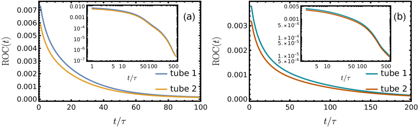
Figure 1: Rate of change of quasi-momentum distributions as a function of time, with Bragg-split states as initial states for the dynamics. Panel $(a)$: intermediate regime, panel (b): strongly interacting regime. In both cases the systems reach the stationary state, with a different timescale for each tube. Insets: the same plots, but for longer times and in logarithmic scale.

The above discussion can be also reinterpreted in the following way. Namely, we can define an aggregate total conserved charge,

$$\mathcal{I}_{\rm total}=\sum_{i=1,2}\int{\rm d}\lambda\,\rho_{\rm p,i}(\lambda)\left(\beta_{2}\lambda^{2}+\sum_{j>2}\beta_{j}f_{i,j}(\lambda)\right),$$ (77)

defined as a specific linear combination of all the conserved charges (49) apart from the particle numbers conserved individually in each tube. The coefficients of this linear combination are the generalized chemical potentials. We make this specific choice for the coefficients because we can compute the single-particle eigenvalue of this total charge from the knowledge of the stationary state. Indeed the expression in the bracket is the bare pseudo-energy of the stationary state up to the chemical potentials $\beta_{i,0}$. Therefore

$$\mathcal{I}_{\rm total}=\int{\rm d}\lambda\left[\left(\epsilon_{1,0}(\lambda)-\beta_{1,0}\right)\rho_{\rm p,1}(\lambda,t)+\left(\epsilon_{2,0}(\lambda)-\beta_{2,0}\right)\rho_{\rm p,2}(\lambda,t)\right].$$ (78)

We will use this formula as a non-trivial check of the existence of conserved charges by solving numerically for the dynamics until we reach the stationary state. We then extract from the stationary state $\epsilon_{i,0}(\lambda)$ and compute with it $\mathcal{I}_{\rm total}$ at each time $t$. If then $\mathcal{I}_{\rm total}$ is indeed time independent, and the stationary state is non-thermal, it means that there are extra conserved charges in the system and the stationary state is the state of maximal entropy constrained by them.

Finally, let us make the following observations. For a single tube Lieb-Liniger model there is a one-to-one relation between the state of the system and chemical potentials. We can now promote this relation to the two-tube case. The state of the system is then described by pseudo-energies $\epsilon_{i}(\lambda)$ given by (71) where now the bare psuedo-energies are

$$\epsilon_{0,i}(\lambda)=\beta_{i,0}+\beta_{i,2}\lambda^{2}+\sum_{j}\beta_{i,j}f_{i,j}(\lambda),$$ (79)

and the temperatures $\beta_{i}$ and chemical potentials $\beta_{i,0}$ are potentially different for the two tubes. For the system evolving according to the Boltzmann equation this leads to a time dependence of the chemical potentials. The stationary state can be then understood as equalization of temperatures and higher chemical potentials, namely $\lim_{t\rightarrow\infty}\left(\beta_{1,j}(t)-\beta_{2,j}(t)\right)=0$ for $j>1$.

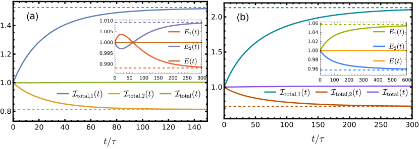
Figure 2: Total charge and energy (insets) as a function of time, for the case of Bragg-split initial states. Panel (a): intermediate interactions, panel (b): strongly interacting regime. To illustrate energy transfer, we plot the energy of both tubes and normalize by the initial values. The same is done for the total charge. While energies and total charges in each tube do change in time, the sum of both contributions is very well conserved.

6 Numerical results

We now numerically solve the Boltzmann equation to demonstrate the main findings of our work. We study relaxation under dynamics restricted to (1,1) processes. We neglect the processes involving more ph pairs effectively considering Eqns. (15) with $Q_{0}\equiv Q_{0}^{(1,1)}$. Moreover, we consider potentials narrow in the momentum space such that $Q_{0}^{(1,1)}$ is very well approximated by its low-momentum limit. With this, we may expect both non-thermal stationary states (56) as the final states of the evolution as well as emergent integrals of motion (59).

To display the athermal character of the stationary states we will compare them with the predictions of the standard Gibbs ensemble (GE). The bare psuedoenergies are then

$$\epsilon_{0,i}(\lambda)=\beta_{i,0}+\beta_{2}\lambda^{2},$$ (80)

with $\beta_{1,0},\beta_{2,0}$ and $\beta_{2}$ fixed by the initial densities in both tubes and their total energy.

6.1 Bragg-split states

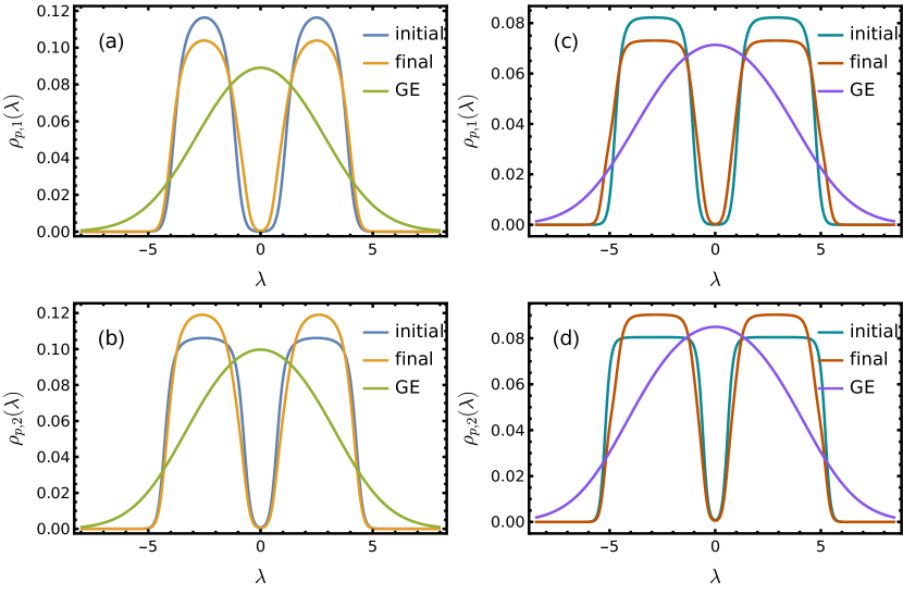
Figure 3: Initial, final and GE states for the dynamics with Bragg-split states as initial states. Panels (a) and (b) present distributions for the simulation in the intermediate regime, whereas in panels (c) and (d) we show the data for the strongly interacting regime. The final states are far from their respective GE states expected to appear as the final, thermal states in a full dynamics involving higher processes.

As initial states, we consider the experimentally relevant Bragg-split thermal distributions [19]. To probe both the intermediate and strong interaction regimes, we perform two computations: one with $c_{1}=2$ and $c_{2}=4$, and one with $c_{1}=32,\,c_{2}=128$. Concretely, we consider initial states of the following form:

$$\rho_{p,i}^{\text{ini}}(\lambda)=\frac{1}{2}\left(\rho^{\text{Gibbs}}_{\beta_{i},\mu_{i}}(\lambda-\lambda_{0})+\rho^{\text{Gibbs}}_{\beta_{i},\mu_{i}}(\lambda+\lambda_{0})\right),$$ (81)

with the parameters used summarized in Table 1.

case 1 (intermediate interactions)							case 2 (strong interactions)
$c_{1}$	$c_{2}$	$\beta_{1}$	$\beta_{2}$	$\mu_{1}$	$\mu_{2}$	$\lambda_{0}$	$c_{1}$	$c_{2}$	$\beta_{1}$	$\beta_{2}$	$\mu_{1}$	$\mu_{2}$	$\lambda_{0}$
2.0	4.0	1.7	1.7	1.35	2.55	2.0	32.0	128.0	1.7	1.7	3.22	5.27	2.9

Table 1: Parameters of the initial states used for the two cases of Bragg-split states explored in this paper.

As the first probe of the relaxation, we investigate the rate of change of the quasiparticle distributions as a function of time defined in the following way

$$\text{ROC}(t)=\frac{\int d\lambda|\partial_{t}\rho_{p}(\lambda;t)|}{\int d\lambda\rho_{p}(\lambda;t)}.$$ (82)

The results are shown at Fig. 1.

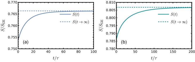
Figure 4: Yang-Yang entropy as a function of time for the dynamics of Bragg-split states. Panel $(a)$: simulation in the intermediate regime, panel $(b)$ dynamics in the strongly interacting regime. The entropy is normalized by the GE prediction for the final state. It reaches a value significantly smaller than 1, indicating that the conserved charges strongly constrain the dynamics.

We observe that the dynamics becomes gradually slower with time and the system reaches a stationary state. The timescales of these processes are different in each tube. This is expected, since couplings and densities differ between the tubes. The dynamics is constrained by the conservation laws.

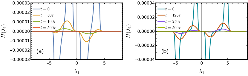
Figure 5: Function $H(\lambda_{1})$ presented as a function of time. Panel (a): intermediate interactions, panel $(b)$ strong interactions. We see that the function approaches zero for late times signalling that the state of the system in this limit fulfills (56).

In Fig. 2 we show that both the energy and the total charge $\mathcal{I}_{\rm tot}$ defined in Eqn. 78 are conserved. We also plot the relative contributions here to these two quantities coming from the two tubes. We can thus observe the flow of energy and $\mathcal{I}_{\rm tot}$ between the two tubes as equilibriation is approached. Importantly, the flow of the total charge between the two tubes is much greater than that of the energy. The final, stationary state reached in the course of $(1,1)$ dynamics is presented in Fig. 3.

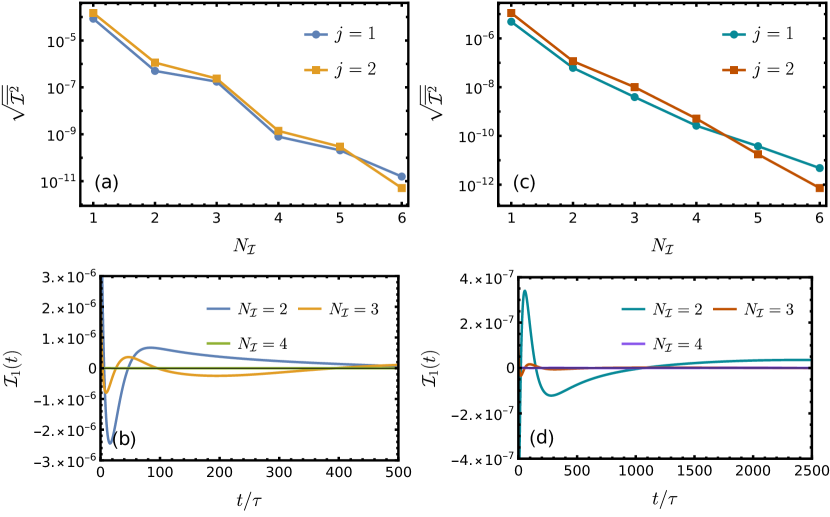
Figure 6: Panels (a) and (c): fluctuations of conserved charges as a function of $N_{\mathcal{I}}$ for $j=1$ and $j=2$. Panels (b) and (d): time evolution of the constructed charge corresponding to $j=1$. We see how the fluctuations drop as $N_{\mathcal{I}}$ is increased. The plots are for the Bragg-split initial states.

We compare in this figure the final particle densities $\rho_{p,i},i=1,2$ to the initial distributions as well as to the predictions of the GE ensemble. We observe that the final, stationary state still resembles a Bragg-split distribution and is very far from the thermal GE state that one would expect from unconstrained dynamics. The impact of the conserved charges on the dynamics is further confirmed as one inspects the Yang-Yang entropy as a function of time as shown in Fig. 4. Due to the additional constraints imposed by the conserved charges, the system relaxes to a state with a much lower entropy in comparison to the prediction computed on the thermal GE state.

Once again we confirm that the system reaches a stationary state that is non-thermal. As a final confirmation, we verify explicitly that the final state fulfills the stationarity condition (56). To do so, we define a function

$$H(\lambda_{1})=\rho_{p,1}(\lambda_{1})\rho_{h,1}(\lambda_{1})\rho_{p,2}(\lambda_{2})\rho_{h,1}(\lambda_{2})\left(\epsilon_{1}^{\prime}(\lambda_{1})-\frac{k_{1}^{\prime}(\lambda_{1})}{k_{2}^{\prime}(\lambda_{2})}\epsilon_{2}^{\prime}(\lambda_{2})\right),$$ (83)

where $\lambda_{2}$ is given by a solution to $v_{1}(\lambda_{1})=v_{2}(\lambda_{2})$ and plot it for several instances of time. If our stationary state is indeed a solution to the Eqn. (56), we should see function $H(\lambda_{1})$ approaching zero at all $\lambda$ for late times. We find that this is the case. In Fig. 5 we see the evolution of function $H$.

Lastly, we construct conserved charges using the algorithm described before in 4.3. For each instance of dynamics we construct two charges, corresponding to $j=1,2$ in (62). We repeat the procedure changing $N_{\mathcal{I}}$, so involving higher order polynomials. We see a roughly exponential decrease of fluctuations with $N_{\mathcal{I}}$, for both charges. This is presented in Figs. 6(a,c). Moreover, in Figs. 6(b,d), we plot the time dependence of the first charge with $j=1$ constructed for different $N_{\mathcal{I}}$. It is clear that the fluctuations of these charges rapidly decrease.

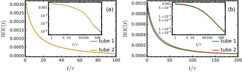
Figure 7: Rate of change of quasi-momentum distributions as a function of time, with thermal states as initial states for the dynamics. Panel $(a)$: intermediate regime, panel (b): strongly interacting regime. In both cases the systems reaches the stationary state, with a different timescale for each tube. Insets: the same plots, but for longer times and in logarithmic scale.

6.2 Two different thermal states

In the second scenario, to probe dynamics closer to an equilibrium state, we consider initial configurations corresponding to thermal states in both tubes. Specifically, the tubes are taken to have the same density $n_{1,2}=1$ but different temperatures. The densities of the initial states read

$$\rho_{p,i}^{\text{ini}}(\lambda)=\rho^{\text{Gibbs}}_{\beta_{i},\mu_{i}}(\lambda),$$ (84)

with the parameters used summarized in Table 2.

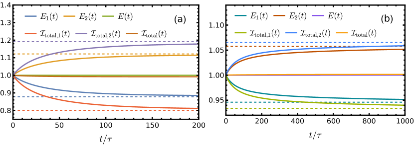
Figure 8: Energy and total charge as a function of time, for the case of thermal initial states. Panel (a): intermediate interactions, panel (b): strongly interacting regime. To illustrate energy transfer, we plot energy of both tubes and normalize by initial values. The same is done for the total charge. The total charge in each tube behaves similarly to the energies, suggesting that $\mathcal{I}_{\rm total}$ consists mostly of the energy of the system and the charges beyond it have small contribution. The dashed lines indicate the asympototic values obtained by the charges and energies.

case 1 (intermediate interations)						case 2 (strong interactions)
$c_{1}$	$c_{2}$	$\beta_{1}$	$\beta_{2}$	$\mu_{1}$	$\mu_{2}$	$c_{1}$	$c_{2}$	$\beta_{1}$	$\beta_{2}$	$\mu_{1}$	$\mu_{2}$
2.0	4.0	0.4	0.7	2.7	4.2	32.0	128.0	0.4	0.7	9.0	9.6

Table 2: Parameters used for the two cases of initial thermal states.

In Fig. 7 we show that the dynamics reaches a stationary point by plotting the ROC of Eqn. (82). In Fig. 8 we show the corresponding evolution of the energy and of the total charge $\mathcal{I}_{\rm total}$. Interestingly, there is a substantial difference between Fig.8 and the corresponding Fig.2 for Bragg-split initial states. For initial thermal states, the flow of the total charge between the two tubes, $\mathcal{I}_{\rm total,1,2}$, is comparable to the flow of the energy in contrast to the Bragg-split initial states. This suggests that the higher conserved charges beyond total energy have a smaller overall contribution to $\mathcal{I}_{\rm total}$ for the case of initial thermal states.

Despite the thermal starting point, the evolution for these states leads to final, non-thermal states that are nonetheless close to thermal states. This is illustrated in Fig. 10 where we compare the distributions $\rho_{\rm p}(\lambda)$ in the initial and final states and in putative thermal equilibrium states consistent with the initial states. The lack of thermalization can be also witnessed in the evolution of the entropy, see Fig. 9. Here we see that the entropy draws close to the equilibrium thermal entropy but does not quite reach it.

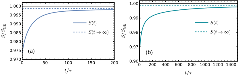
Figure 9: Yang-Yang entropy as a function of time, for the dynamics with initial thermal states. Panel $(a)$: simulation in the intermediate regime, panel $(b)$ dynamics in the strongly interacting regime. The entropy is normalized by the prediction of the GE ensemble for the final state. The final, stationary state is close to a thermal one, which is reflected in value of normalized entropy that is very close to 1.

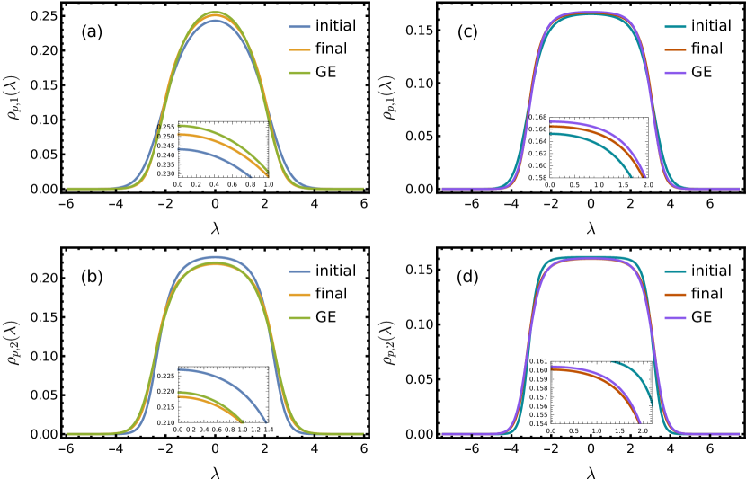
Figure 10: Initial, final and GE states for the dynamics with thermal states as initial states. Panels (a) and (b) present distributions for the simulation in the intermediate regime, whereas in panels (c) and (d) we show the data for strongly interacting regime. Final distributions are very close to the predictions of the GE, indicating that the system has almost thermalized. The small but real differences between the final and putative thermal distributions are clearly seen in the insets, where we have plotted the behavior of the distributions near $\lambda=0$.

The two kinds of initial states that we have considered show certain universal features of the dynamics generated by the (1,1) processes for long range interactions. The first observation that we can make is that these processes are not very efficient in redistributing the particles in the tubes. This, on one hand, is reflected in the existence of higher conserved charges. On more practical level it results in small changes to the particles distributions with the stationary states very similar to the initial states. This is true for both Bragg-split and the thermal initial states.

7 Summary and Conclusion

In this work we have studied the problem of the development of stationary states in a weakly perturbed integrable model. Our approach relies on a microscopic scattering integral in the framework of a Boltzmann equation. We applied this approach to the case of two weakly coupled Lieb-Liniger models, with the coupling taking the form of the density-density interactions, a scenario relevant for the experiments with ultra-cold atomic gases. We found that for the long-range intertube interactions the leading processes described by the scattering integral do not thermalize the system. Instead they lead to an athermal state which can be characterized by a generalized Gibbs ensemble. We provided a numerical construction of the intricate conserved charges responsible for the lack of thermalization and showed that the evolution of the system displays extra conserved charges beyond the particle number, momentum, and energy. To further understand the resulting time evolution we have solved numerically the Boltzmann equation for two very different initial states: i) the highly non-equilibrium Bragg split states and i) tubes characterized by thermal states at different temperatures. In both cases we have observed that the presence of the extra conserved charges greatly restricts the time evolution. The final stationary states resemble the initial states and do not evolve into thermal states. We also witnessed this arrested dynamics through studying the entropy production. There we saw that the system’s entropy would evolve to a value lower than that of a thermal ensemble.

In this work we have focused on revealing the structure of the athermal stationary states. An interesting question would be to combine the leading $(1,1)$ with higher processes that do thermalize the system. This would provide an access to the full time evolution from the initial state, through the prethermalization plateau, all the way to the final thermal state. Numerical implementation of this problem requires a substantial effort that we delegate to future work.

Our work leads also to a more fundamental question whether the extra conserved charges exist at the quantum level, beyond the Boltzmann equation. Whereas their exact conservation is unlikely, one might conjecture that they correspond to ’slow variables’ and therefore they remain important for the dynamics at intermediate timescales. Coupled spin chains, or ladder systems, provide a convenient setup in which to study such questions. Here density matrix renormalization group based methods can be used to study the full quantum dynamics. We shall address this in future publications.

Finally, the results for the case where the two tubes are initialized in thermal states at different temperatures shows that the evolution occurs entirely in the vicinity of thermal states. In such a situation it might be possible to develop an effective description of the dynamics which instead of looking at the full distribution of the rapidities would involve only examining the evolution of the temperatures and perhaps several of the higher chemical potentials. This would then allow the development of a sort of Newton’s law of cooling for weakly perturbed integrable systems.

Appendix A Scaling of the collision integral in the small momentum limit

In this appendix we show that $Q_{0}^{(m,n)}\sim k_{r}^{m+n}$ with $k_{r}$ the characteristic momentum of the intertube potential. From the symmetry of Eqn. (29), we can replace sum of delta functions by a single one, multiplied by $n$

$$Q_{0}^{(n,m)}[\rho_{p,1},\rho_{p,2}](\lambda)= (2\pi)^{2}n\int d\mathbf{p}_{1}^{n}d\mathbf{h}_{1}^{n}d\mathbf{p}_{2}^{m}d\mathbf{h}_{2}^{m}\,\delta(\lambda-p_{1,1})\,\tilde{A}^{2}\big{(}k_{1}(\mathbf{p}_{1},\mathbf{h}_{1})\big{)}\,\times$$ (85)

$$\times|F_{1}(\mathbf{p}_{1},\mathbf{h}_{1})|^{2}|F_{2}(\mathbf{p}_{2},\mathbf{h}_{2})|^{2}\mathcal{J}^{(n,m)}(\mathbf{p}_{1},\mathbf{h}_{1},\mathbf{p}_{2},\mathbf{h}_{2})$$

$$\times\delta\big{(}k_{1}(\mathbf{p}_{1},\mathbf{h}_{1})+k_{2}(\mathbf{p}_{2},\mathbf{h}_{2})\big{)}\,\delta\big{(}\omega_{1}(\mathbf{p}_{1},\mathbf{h}_{1})+\omega_{2}(\mathbf{p}_{2},\mathbf{h}_{2})\big{)},$$

where we recall the definition of $\mathcal{J}^{(n,m)}$

$$\mathcal{J}^{(n,m)}(\mathbf{p}_{1},\mathbf{h}_{1},\mathbf{p}_{2},\mathbf{h}_{2})=J_{1}^{n}(\mathbf{p}_{1},\mathbf{h}_{1})\,J_{2}^{m}(\mathbf{p}_{2},\mathbf{h}_{2})-J_{1}^{n}(\mathbf{h}_{1},\mathbf{p}_{1})\,J_{2}^{m}(\mathbf{h}_{2},\mathbf{p}_{2}).$$ (86)

We express the collision integrals in the center of mass variables, namely,

$$\lambda_{i,j}=\frac{1}{2}(p_{i,j}+h_{i,j})\qquad\alpha_{i,j}=p_{i,j}-h_{i,j}.$$ (87)

We make now the following observations. The form-factors of the density operator, due to their ph symmetry are even function of $\alpha_{i,j}$ and their leading order is $\alpha_{i,j}$ independent, i.e.,

$$F_{1}(\mathbf{p}_{1},\mathbf{h}_{1})=F_{1}(\bm{\lambda}_{1},\bm{\lambda}_{1})+\mathcal{O}(\alpha_{i}^{2}).$$ (88)

The difference of the density factors appearing through the $J$ functions, see (24), is an odd function upon changing the sign of all $\alpha_{i,j}$. At the same time, the product of the density functions evaluated for a particle-hole excitation gives

$$\rho_{p}(\lambda-\alpha/2)\rho_{h}(\lambda+\alpha/2)=\rho_{p}(\lambda)\rho_{h}(\lambda)\left(1+\epsilon^{\prime}(\lambda)\alpha/2+\mathcal{O}(\alpha^{2})\right).$$ (89)

Therefore we get

$$\mathcal{J}^{(n,m)}(\mathbf{p}_{1},\mathbf{h}_{1},\mathbf{p}_{2},\mathbf{h}_{2}) =\prod_{i=1}^{n}\rho_{p,1}(\lambda_{i,1})\rho_{h,1}(\lambda_{i,1})\prod_{j=1}^{m}\rho_{p,2}(\lambda_{j,2})\rho_{h,2}(\lambda_{j,2})\times$$ (90)

$$\left(\sum_{i=1}^{n}\epsilon_{1}^{\prime}(\lambda_{1,i})\alpha_{1,i}+\sum_{i=1}^{m}\epsilon_{2}^{\prime}(\lambda_{2,i})\alpha_{2,i}+\mathcal{O}(\alpha_{i,j}^{3})\right).$$

The scattering integral, up to the first two leading orders in $\alpha_{i,j}$, takes then the following form,

$$Q_{0}^{(n,m)}[\rho_{p,1},\rho_{p,2}](\mu)=(2\pi)^{2}n\int d\bm{\lambda}_{1}^{n}d\bm{\lambda}_{2}^{m}G(\bm{\lambda}_{1},\bm{\lambda}_{2})H(\bm{\lambda}_{1},\bm{\lambda}_{2}),$$ (91)

where

$$G(\bm{\lambda}_{1},\bm{\lambda}_{2}) =|F_{1}(\bm{\lambda}_{1},\bm{\lambda}_{1})|^{2}|F_{2}(\bm{\lambda}_{2},\bm{\lambda}_{2})|^{2}\prod_{i=1}^{n}\rho_{p,1}(\lambda_{i,1})\rho_{h,1}(\lambda_{i,1})\prod_{j=1}^{m}\rho_{p,2}(\lambda_{j,2})\rho_{h,2}(\lambda_{j,2}),$$ (92)

$$H(\bm{\lambda}_{1},\bm{\lambda}_{2}) =\int d\bm{\alpha}_{1}^{n}d\bm{\alpha}_{2}^{m}\tilde{A}^{2}(k_{1}(\mathbf{p}_{1},\mathbf{h}_{1}))\delta(\mu-\lambda_{1,1}-\alpha_{1,1}/2)\delta\big{(}k_{1}(\mathbf{p}_{1},\mathbf{h}_{1})+k_{2}(\mathbf{p}_{2},\mathbf{h}_{2})\big{)}\,$$

$$\times \delta\big{(}\omega_{1}(\mathbf{p}_{1},\mathbf{h}_{1})+\omega_{2}(\mathbf{p}_{2},\mathbf{h}_{2})\big{)}\left(\sum_{i=1}^{n}\epsilon_{1}^{\prime}(\lambda_{1,i})\alpha_{1,i}+\sum_{i=1}^{m}\epsilon_{2}^{\prime}(\lambda_{2,i})\alpha_{2,i}\right).$$ (93)

Consider first the simplest case of $(1,1)$ processes. Then we have to perform the following integral

$$H(\lambda_{1},\lambda_{2}) =\int{\rm d}\alpha_{1}{\rm d}\alpha_{2}\,\tilde{A}^{2}(k_{1}(\lambda_{1},\alpha_{1}))\delta(\mu-\lambda_{1}-\alpha_{1}/2)\delta\big{(}k_{1}(\lambda_{1},\alpha_{1})+k_{2}(\lambda_{2},\alpha_{2})\big{)}\,$$

$$\times \delta\big{(}\omega_{1}(\lambda_{1},\alpha_{1})+\omega_{2}(\lambda_{2},\alpha_{2}\big{)}\left(\epsilon_{1}^{\prime}(\lambda_{1})\alpha_{1}+\epsilon_{2}^{\prime}(\lambda_{2})\alpha_{2}\right).$$ (94)

For the momentum energy constraints we find

$$k(\lambda,\alpha)=\alpha k^{\prime}(\lambda)+\mathcal{O}(\alpha^{3}),\qquad\omega(\lambda,\alpha)=\alpha\omega^{\prime}(\lambda)+\mathcal{O}(\alpha^{3}).$$ (95)

Thus we have

$$\delta\big{(}k_{1}(\lambda_{1},\alpha_{1})+k_{2}(\lambda_{2},\alpha_{2})\big{)}=\delta(\alpha_{1}k_{1}^{\prime}(\lambda_{1})+\alpha_{2}k_{2}^{\prime}(\lambda_{2})),$$ (96)

and similarly for the energy $\delta$-function. Then we can write

$$\delta\big{(}k_{1}(\lambda_{1},\alpha_{1})+k_{2}(\lambda_{2},\alpha_{2})\big{)}\,\delta\big{(}\omega_{1}(\lambda_{1},\alpha_{1})+\omega_{2}(\lambda_{2},\alpha_{2}\big{)} =$$ (99)

$$\hskip-216.81pt\frac{\delta(\alpha_{2}+\alpha_{1}k_{1}^{\prime}(\lambda_{1})/k_{2}^{\prime}(\lambda_{2}))}{|\alpha_{1}k_{1}^{\prime}(\lambda_{1})k_{2}^{\prime}(\lambda_{2})|}\delta(v_{1}(\lambda_{1})-v_{2}(\lambda_{2})),$$

where $v(\lambda)=\omega^{\prime}(\lambda)/k^{\prime}(\lambda)$. We can perform now the integral over $\alpha_{2}$. The result is

$$H(\lambda_{1},\lambda_{2})= \int{\rm d}\alpha_{1}\,{\rm sgn}(\alpha_{1})\tilde{A}^{2}(k_{1}(\lambda_{1},\alpha_{1}))\delta(\mu-\lambda_{1}-\alpha_{1}/2)\times$$ (100)

$$\frac{\delta(v_{1}(\lambda_{1})-v_{2}(\lambda_{2}))}{|k_{2}^{\prime}(\lambda_{2})|}\left(\frac{\epsilon_{1}^{\prime}(\lambda_{1})}{k_{1}^{\prime}(\lambda_{1})}-\frac{\epsilon_{2}^{\prime}(\lambda_{2})}{k_{2}^{\prime}(\lambda_{2})}\right).$$ (101)

The remaining integral over $\alpha_{1}$ can be now also performed. The result is

$$H(\lambda_{1},\lambda_{2})={\rm sgn}(\mu-\lambda_{1})\tilde{A}^{2}(k_{1}(\lambda_{1},2(\mu-\lambda_{1})))\frac{\delta(v_{1}(\lambda_{1})-v_{2}(\lambda_{2}))}{|k_{2}^{\prime}(\lambda_{2})|}\left(\frac{\epsilon_{1}^{\prime}(\lambda_{1})}{k_{1}^{\prime}(\lambda_{1})}-\frac{\epsilon_{2}^{\prime}(\lambda_{2})}{k_{2}^{\prime}(\lambda_{2})}\right).$$ (102)

The remaining $\delta$-function fixes uniquely $\lambda_{2}$ as a function of $\lambda_{1}$. Therefore the scattering integral involves only one integral. The range of the integration over $\lambda_{1}$ is constrained by the function $\tilde{A}(k_{1}(\lambda_{1},2(\mu-\lambda_{1}))$ which is peaked around $\lambda_{1}=\mu$. The structure of the expression is then

$$Q_{0}^{(1,1)}[\rho_{p,1},\rho_{p,2}](\mu)=\int{\rm d}\lambda_{1}{\rm sgn}(\mu-\lambda_{1})\tilde{A}^{2}(2(\mu-\lambda_{1})k^{\prime}(\lambda_{1}))f(\lambda_{1}),$$ (103)

where in $f(\lambda_{1})$ we have gathered all the remaining factors. Now we will take advantage of properties of the interaction potential and use representation (21). We get

$$Q_{0}^{(1,1)}[\rho_{p,1},\rho_{p,2}](\mu)\sim\int{\rm d}\lambda_{1}\,{\rm sgn}(\mu-\lambda_{1})\tilde{a}^{2}\left(\frac{2(\mu-\lambda_{1})k^{\prime}(\lambda_{1})}{k_{r}}\right)f(\lambda_{1}).$$ (104)

We assume now that function $\tilde{a}(k/k_{r})$ is centered around $0$ and symmetric. In the leading order in $k_{r}$ we can approximate this expression by replacing $k^{\prime}(\lambda_{1})$ by $k^{\prime}(\mu)$. We then change the variables to $x=2(\mu-\lambda_{1})k^{\prime}(\mu)/k_{r}$. The result is

$$Q_{0}^{(1,1)}[\rho_{p,1},\rho_{p,2}](\mu)\sim\frac{k_{r}}{2k^{\prime}(\mu)}\int{\rm d}x\,{\rm sgn}(x)\tilde{a}^{2}(x)f\left(\mu-x\frac{k_{r}}{2k^{\prime}(\mu)}\right).$$ (105)

Expanding now in powers of $x$ we find

$$Q_{0}^{(1,1)}[\rho_{p,1},\rho_{p,2}](\mu)\sim\frac{k_{r}f(\mu)}{2k^{\prime}(\mu)}\int{\rm d}x\,{\rm sgn}(x)\tilde{a}^{2}(x)+\frac{k_{r}^{2}f^{\prime}(\mu)}{(2k^{\prime}(\mu))^{2}}\int{\rm d}x\,|x|\tilde{a}(x)+\mathcal{O}(k_{r}^{4}).$$ (106)

The first integral vanishes and the leading contribution comes from the second term which is proportional to the characteristic momentum $k_{r}$. The answer involves the derivative of $f(\mu)$. This function involves all the density factors and form-factors. Its derivative is thus quite complicated and not very practical for numerical computations. We also note that the subleading corrections are of order $k_{r}^{4}$ and not $k_{r}^{2}$ which is important for the hierarchy of processes contributing to the Boltzmann equation as discussed in the main text.

We generalize now the analysis to the $(n,m)$ case. We start by considering $H(\bm{\lambda}_{1},\bm{\lambda}_{2})$ and use the energy-momentum constraints to solve for $\alpha_{m,2}$ and $\lambda_{m,2}$ and the third $\delta$-function to fix $\lambda_{1,1}=\mu-\alpha_{1,1}/2$. To this end we introduce the following notation

$$\bar{k} =\sum_{i=1}^{n}\alpha_{i,1}k_{1}^{\prime}(\lambda_{i,1})+\sum_{i=1}^{m-1}\alpha_{i,2}k_{2}^{\prime}(\lambda_{i,2}),$$ (107)

$$\bar{\omega} =\sum_{i=1}^{n}\alpha_{i,1}\omega_{1}^{\prime}(\lambda_{i,1})+\sum_{i=1}^{m-1}\alpha_{i,2}\omega_{2}^{\prime}(\lambda_{i,2}),$$ (108)

$$\bar{\epsilon} =\sum_{i=1}^{n}\alpha_{i,1}\epsilon_{1}^{\prime}(\lambda_{i,1})+\sum_{i=1}^{m-1}\alpha_{i,2}\epsilon_{2}^{\prime}(\lambda_{i,2}),$$ (109)

and $\bar{v}=\bar{\omega}/\bar{k}$. Then

$$\delta\big{(}k_{1}(\mathbf{p}_{1},\mathbf{h}_{1})+k_{2}(\mathbf{p}_{2},\mathbf{h}_{2})\big{)}\delta\big{(}\omega_{1}(\mathbf{p}_{1},\mathbf{h}_{1})+\omega_{2}(\mathbf{p}_{2},\mathbf{h}_{2})\big{)}=\frac{\delta(\alpha_{m,2}-\bar{\alpha}_{m,2})\delta(v_{2}(\lambda_{m,2})-\bar{v})}{k^{\prime}(\lambda_{m,2})|\bar{k}|},$$ (110)

with $\bar{\alpha}_{m,2}=\bar{k}/k_{2}^{\prime}(\lambda_{m,2})$. This gives

$$H(\bm{\lambda}_{1},\bm{\lambda}_{2}) =\int d\bm{\alpha}_{1}^{n}d\bm{\alpha}_{2}^{m-1}\tilde{A}^{2}(k_{1}(\mathbf{p}_{1},\mathbf{h}_{1}))\frac{\delta(v_{2}(\lambda_{1,2})-\bar{v})}{k^{\prime}(\lambda_{1,2})}\left(\frac{\bar{\epsilon}}{\bar{k}}-\frac{\epsilon_{2}^{\prime}(\lambda_{1,2})}{k_{2}^{\prime}(\lambda_{1,2})}\right){\rm sgn}(\bar{k}).$$ (111)

We now introduce new variables $x_{i,j}=\alpha_{i,j}k^{\prime}(\lambda_{i,j})/k_{r}$ for all $i,j$ except for $i=j=1$ where we write instead $x_{1,1}=\alpha_{1,1}k^{\prime}(\mu))/k_{r}$. We now find for $H(\bm{\lambda}_{1},\bm{\lambda}_{2})$,

$$H(\bm{\lambda}_{1},\bm{\lambda}_{2}) =k_{r}^{n+m-1}\frac{\delta(v_{2}(\lambda_{1,2})-\bar{v})}{\prod_{i,j}k^{\prime}(\lambda_{i,j})}\int d\bm{x}_{1}^{n}d\bm{x}_{2}^{m-1}{\rm sgn}(\sum_{i,j}x_{i,j})\tilde{a}^{2}\left(\sum_{i}x_{i,1}\right)\left(\frac{\bar{\epsilon}}{\bar{k}}-\frac{\epsilon_{2}^{\prime}(\lambda_{m,2})}{k_{2}^{\prime}(\lambda_{m,2})}\right).$$ (112)

In writing the argument of $\tilde{a}$ we have neglected contributions of order $x_{1,1}^{2}$ as they do not contribute to the integral in the first two leading orders. The ratio $\bar{\epsilon}/\bar{k}$ is the following

$$\frac{\bar{\epsilon}}{\bar{k}}=\frac{\sum x_{i,j}\epsilon_{j}^{\prime}(\lambda_{i,j})/k_{j}^{\prime}(\lambda_{i,j})+x_{1,1}\epsilon_{1}^{\prime}(\mu-\alpha_{1,1}/2)/k_{1}^{\prime}(\mu))}{\sum x_{i,j}+x_{1,1}k_{1}^{\prime}(\mu-\alpha_{1,1}/2)/k_{1}^{\prime}(\mu)},$$ (113)

with $\alpha_{1,1}=k_{r}x_{1,1}/k_{1}^{\prime}(\mu)$. Thus at the leading order in $k_{r}$ it is $k_{r}$ independent and invariant under simultaneous change of sign of all the $x_{i,j}$. Therefore the integral over all the $x_{i,j}$’s vanishes. The leading contribution comes then from including the correction due to $\alpha_{1,1}$. Therefore, the whole contribution to the scattering integral is of the order $k_{r}^{n+m}$ as stated in the main text.

Appendix B Absence of non-thermal stationary states beyond the small momentum limit

In the main body of the text we demonstrated that if the dynamics of the two tubes of gas are controlled by $(1,1)$ processes in the small momentum limit, a prethermalization plateau is arrived at that is characterized by a set of non-trivial conservation laws. In this appendix, we argue that this is in general a special case, that if we consider $(1,1)$ processes outside a small momentum approximation, thermalization occurs. We note up front that there are two exceptions to this general rule:

• The Tonks-Girardeau (TG) limit. The thermalization that occurs due to the higher momentum $(1,1)$ processes happens because of non-linearities in the dispersion relation induced by interactions. But at $c=\infty$ these interactions are absent and the argument for a non-trivial prethermalization plateau continues to hold even if higher momentum processes are accounted for. Moreover we can conclude that TG gases do not thermalize at all as higher-order ph processes are absent. Though we have broken the integrability at the level of a single tube, new exact integrals of motion have appeared for the two-tube case.

• The two gases are identical. In this case the $(1,1)$ processes induces no dynamics whatsoever and the gas does not evolve. Thermalization however will still happen on account of higher order $(n,m)$ processes.

We will comment on these two special cases further.

So let us turn to $(1,1)$ processes at arbitrary momentum. The condition for the stationary state, $Q_{0}^{(1,1)}=0$, translates to demanding that

$$\epsilon_{1}(p_{1})-\epsilon_{1}(h_{1})+\epsilon_{2}(p_{2})-\epsilon_{2}(h_{2})=0,$$ (114)

for all $p_{1},h_{1},p_{2},h_{2}$ fulfilling the momentum-energy constraints

$$\begin{split}k_{1}(p_{1})-k_{1}(h_{1})+k_{2}(p_{2})-k_{2}(h_{2})&=0,\\ \omega_{1}(p_{1})-\omega_{1}(h_{1})+\omega_{2}(p_{2})-\omega_{2}(h_{2})&=0.\end{split}$$ (115)

Here functions $k_{i}(\lambda)$ and $\omega_{i}(\lambda)$ are determined from the $\epsilon_{i}(\lambda)$ through the TBA equations. We start by analyzing the structure of Eqns. (114) and (115).

The constraints (115) can be solved for $p_{1}$ and $h_{1}$. We assume that the solution is unique and takes the form $p_{1}=f(p_{2},h_{2})$ and $h_{1}=g(p_{2},h_{2})$ for two functions $f$ and $g$. Because of the symmetry of the constraints upon replacing particles with holes the two functions are not independent and we have $g(p_{2},h_{2})=f(h_{2},p_{2})$. Therefore, a generic solution to the constraints can be written as

$$p_{1}=f(p_{2},h_{2}),\quad h_{1}=f(h_{2},p_{2}).$$ (116)

We define now a function $F(p_{2},h_{2})$,

$$F(p_{2},h_{2})\equiv\epsilon_{1}(f(p_{2},h_{2}))-\epsilon_{1}(f(h_{2},p_{2})).$$ (117)

The condition (114) for the stationary state in these terms is simply

$$F(p_{2},h_{2})=\epsilon_{2}(p_{2})-\epsilon_{2}(h_{2}).$$ (118)

To obtain a general solution here we assume that $f(p_{2},h_{2})$ is independent of one of its variables, which we choose to be $p_{2}$. This simplifies the structure of $F$ to

$$F(p_{2},h_{2})=\epsilon_{1}(f(h_{2}))-\epsilon_{1}(f(p_{2})).$$ (119)

The equation for the stationary states separates now in two parts depending only on $p_{2}$ and $h_{2}$ respectively. This leads to two independent equations of the same form which fixes the relation between $\epsilon_{1}$ and $\epsilon_{2}$ up to an additive constant which is just a difference of chemical potentials. The result is

$$\epsilon_{1}(f(\lambda))=\epsilon_{2}(\lambda)+\mu_{1}-\mu_{2}.$$ (120)

The function $f(\lambda)$ by construction satisfies

$$k_{1}(f(p_{2}))-k_{1}(f(h_{2}))+k_{2}(p_{2})-k_{2}(h_{2}) =0,$$ (121)

$$\omega_{1}(f(p_{2}))-\omega_{1}(f(h_{2}))+\omega_{2}(p_{2})-\omega_{2}(h_{2}) =0.$$ (122)

Assuming the monotonicity of the dressed momenta $k_{i}$, it is straightforward to solve the first equation for $f$. The result is $f=k_{1}^{-1}\circ k_{2}$. The second equation provides now a constraint between the functions $k_{i}$ and $\omega_{i}$ themselves. It reads

$$\omega_{2}\circ k_{2}^{-1}=\omega_{1}\circ k_{1}^{-1}.$$ (123)

Putting it all together we find the following set of equations

$$\begin{split}\epsilon_{1}\circ k_{1}^{-1}(p)-\mu_{1}&=\epsilon_{2}(p)\circ k_{2}^{-1}(p)-\mu_{2},\\ \omega_{1}\circ k_{1}^{-1}(p)&=\omega_{2}\circ k_{2}^{-1}(p).\end{split}$$ (124)

This is a sought after rewriting of equations (114) and (115). For a given function $\epsilon_{2}$, the TBA equations determine $k_{2}$ and $\omega_{2}$. Thus the right hand sides of the above two equations are known. The equations then have to be solved for $\epsilon_{1}$ such that TBA integral equations defining $k_{1}$ and $\omega_{1}$ in terms of $\epsilon_{1}$ are self-consistent.

We show now three special cases where we can solve the above:

• Thermal states: For a thermal state in the second tube, $\epsilon_{2}(\lambda)=\mu_{2}+\beta\omega_{2}(\lambda)$, we have a chain of following transformations

  $$\epsilon_{1}\circ k_{1}^{-1}(p)-\mu_{1} =\epsilon_{2}\circ k_{2}^{-1}(p)-\mu_{2}$$ (125)

  $$=\beta\omega_{2}\circ k_{2}^{-1}(p)$$ (126)

  $$=\beta\omega_{1}\circ k_{1}^{-1}(p).$$ (127)

  Therefore the solution is $\epsilon_{1}(\lambda)=\mu_{1}+\beta\omega_{1}(\lambda)$ and we know that this choice is consistent with the TBA integrals defining $\omega_{1}$ and $k_{1}$.

• Identical gases in identical states: If the two tubes of gas are identical in all respects, then any choice of $\epsilon_{1}=\epsilon_{2}$ (both thermal and athermal) satisfies the above conditions. Because $k_{1}=k_{2}$ and $\omega_{1}=\omega_{2}$, any scattering process must have $p_{1}=h_{2}$ and $p_{2}=h_{1}$. By symmetry under exchange of particles and holes, $Q^{1,1}$ vanishes identically and at this order, the gas does not evolve from its initial state.

• Tonks-Girardeau gas: When both tubes are in the strongly interacting limit, $c_{i}=\infty$, then there is no dressing and the second equality in (124) is trivially fulfilled. At the same time the first equations simplifies to $\epsilon_{1}(\lambda)-\mu_{1}=\epsilon_{2}(\lambda)-\mu_{2}$. Therefore the stationary state is given by the pseudo-energies equal up to the chemical potentials which can be different in both tubes.

We cannot prove that other solutions are impossible, but we were unable to find additional possibilities. Therefore we expect that in general the higher momentum contributions to the $(1,1)$ processes lead to the thermalization of the system.

Further support of this contention is provided by considering an expansion of the stationary state condition in the momentum transferred between the states. To this end we expand eqs. (114) and (115) in $\alpha_{i}=p_{i}-h_{i}$. At leading order we obtain the following constraint:

$${\rm v}_{1}(\lambda_{1}) = {\rm v}_{2}(\lambda_{2});$$ (128)

$$\epsilon_{1}^{\prime}(\lambda_{1}) = \frac{k^{\prime}_{1}(\lambda_{1})}{k^{\prime}_{2}(\lambda_{2})}\epsilon^{\prime}_{2}(\lambda_{2}),$$ (130)

where $\lambda_{i}=\frac{1}{2}(p_{i}+h_{i})$. We already know that these constraints admit solutions that are athermal. This was our main result in the main body of the text. At next order in $\alpha_{i}$, ${\cal O}(\alpha_{i}^{3})$, we obtain additional constraints that need to be satisfied for stationarity:

$${\rm v}_{2}(\lambda_{1}) = \bigg{(}1-\frac{k^{\prime}_{1}(\lambda_{1})^{3}}{k^{\prime}_{2}(\lambda_{2})^{3}}\frac{k^{\prime\prime\prime}_{2}(\lambda_{2})}{k^{\prime\prime\prime}_{1}(\lambda_{1}))}\bigg{)}^{-1}\bigg{(}\frac{\omega^{\prime\prime\prime}_{1}(\lambda_{1})}{k^{\prime\prime\prime}_{1}(\lambda_{1})}-\frac{k^{\prime}_{1}(\lambda_{1})^{3}}{k^{\prime}_{2}(\lambda_{2})^{3}}\frac{\omega^{\prime\prime\prime}_{2}(\lambda_{2})}{k^{\prime\prime\prime}_{1}(\lambda_{1})}\bigg{)};$$ (131)

$$\epsilon_{1}^{\prime\prime\prime}(\lambda_{1}) = \bigg{(}\frac{k^{\prime\prime\prime}_{1}(\lambda_{1})}{k^{\prime}_{2}(\lambda_{2})}-\frac{k^{\prime}_{1}(\lambda_{1})^{3}}{k^{\prime}_{2}(\lambda_{2})^{4}}k^{\prime\prime\prime}_{2}(\lambda_{2})\bigg{)}\epsilon^{\prime}_{2}(\lambda_{2})+\frac{k^{\prime}_{1}(\lambda_{1})^{3}}{k^{\prime}_{2}(\lambda_{2})^{3}}\epsilon^{\prime\prime\prime}_{2}(\lambda_{2}).$$ (133)

It seems unlikely that both constraints (128) and (131) can be satisfied simultaneously, beyond the specialized circumstances discussed above. A similar line of reasoning may be straightforwardly extended to processes involving more ph pairs.

Appendix C Perturbative solution of the stationary state equation

In this Appendix we solve equation (56) for the stationary state in the limit of large couplings $c_{i}$ in both tubes. We start with the expressions for the dressing procedure (12). The kernel becomes constant $T(\lambda)=1/(\pi c)+\mathcal{O}(1/c^{3})$ and

$$f_{\rm dr}(\lambda)=f(\lambda)+\frac{1}{\pi c}\int{\rm d}\mu\,n(\mu)f_{\rm dr}(\mu)+\mathcal{O}(1/c^{3}).$$ (134)

This equation can be solved iteratively. Including the leading correction in $1/c$ we find

$$f_{\rm dr}(\lambda)=f(\lambda)+\frac{1}{\pi c}\int{\rm d}\mu\,n(\mu)f(\mu)+\mathcal{O}(1/c^{2}).$$ (135)

From (9a) we find

$$k^{\prime}(\lambda)=1-\frac{2n}{c}+\mathcal{O}(1/c^{2}),$$ (136)

where we used that $n(\lambda)=\rho_{\rm p}(\lambda)/(2\pi)+\mathcal{O}(1/c)$ and denoted by $n=\int{\rm d}\lambda\rho_{\rm p}(\lambda)$. For the derivative of the dressed energy we find

$$\omega^{\prime}(\lambda)=2\lambda+\mathcal{O}(1/c^{2}),$$ (137)

where we assumed that $n(\lambda)$ is an even function of $\lambda$. We note that, up to the first order in $1/c$, the dressing influences only even functions of the rapidity. The effective velocity, defined as $v(\lambda)=\omega^{\prime}(\lambda)/k^{\prime}(\lambda)$, is then

$$v(\lambda)=2\lambda\left(1+\frac{2n}{c}\right).$$ (138)

In the large $c$ limit, the stationary state equation (56) takes the following form

$$\epsilon_{1}^{\prime}(\lambda_{1})\left(1+\frac{2n_{1}}{c_{1}}\right)=\epsilon_{2}^{\prime}(\lambda_{2})\left(1+\frac{2n_{2}}{c_{2}}\right),\qquad\lambda_{1}\left(1+\frac{2n_{1}}{c_{1}}\right)=\lambda_{2}\left(1+\frac{2n_{2}}{c_{2}}\right).$$ (139)

Therefore for any function $\epsilon_{1}(\lambda)$ describing the gas in the first tube, we can find $\epsilon_{2}(\lambda)$ such that

$$\epsilon_{2}^{\prime}(\lambda)=\zeta^{-1}\epsilon_{1}^{\prime}\left(\zeta\lambda\right),\qquad\zeta=\frac{1+\frac{2n_{2}}{c_{2}}}{1+\frac{2n_{1}}{c_{1}}}.$$ (140)

The state of the system characterized by $\epsilon_{1}(\lambda)$ and $\epsilon_{2}(\lambda)$ is then stationary.

References

- [1] A. Polkovnikov, K. Sengupta, A. Silva and M. Vengalattore, Colloquium: Nonequilibrium dynamics of closed interacting quantum systems, Rev. Mod. Phys. 83, 863 (2011), 10.1103/RevModPhys.83.863.
- [2] C. Gogolin and J. Eisert, Equilibration, thermalisation, and the emergence of statistical mechanics in closed quantum systems, Reports on Progress in Physics 79(5), 056001 (2016), 10.1088/0034-4885/79/5/056001.
- [3] L. D’Alessio, Y. Kafri, A. Polkovnikov and M. Rigol, From quantum chaos and eigenstate thermalization to statistical mechanics and thermodynamics, Advances in Physics 65(3), 239 (2016).
- [4] J. M. Deutsch, Quantum statistical mechanics in a closed system, Phys. Rev. A 43, 2046 (1991), 10.1103/PhysRevA.43.2046.
- [5] M. Srednicki, Chaos and quantum thermalization, Phys. Rev. E 50, 888 (1994), 10.1103/PhysRevE.50.888.
- [6] M. Srednicki, Thermal fluctuations in quantized chaotic systems, Journal of Physics A: Mathematical and General 29(4), L75 (1996), 10.1088/0305-4470/29/4/003.
- [7] M. Srednicki, The approach to thermal equilibrium in quantized chaotic systems, Journal of Physics A: Mathematical and General 32(7), 1163 (1999), 10.1088/0305-4470/32/7/007.
- [8] M. Rigol, V. Dunjko and M. Olshanii, Thermalization and its mechanism for generic isolated quantum systems, Nature 452(7189), 854 (2008), 10.1038/nature06838.
- [9] S. Moudgalya, B. A. Bernevig and N. Regnault, Quantum many-body scars and Hilbert space fragmentation: a review of exact results, Reports on Progress in Physics 85(8), 086501 (2022), 10.1088/1361-6633/ac73a0.
- [10] M. Serbyn, D. A. Abanin and Z. Papić, Quantum many-body scars and weak breaking of ergodicity, Nature Physics 17(6), 675 (2021), 10.1038/s41567-021-01230-2.
- [11] C. J. Turner, A. A. Michailidis, D. A. Abanin, M. Serbyn and Z. Papić, Weak ergodicity breaking from quantum many-body scars, Nature Physics 14(7), 745 (2018), 10.1038/s41567-018-0137-5.
- [12] A. J. A. James, R. M. Konik and N. J. Robinson, Nonthermal states arising from confinement in one and two dimensions, Phys. Rev. Lett. 122, 130603 (2019), 10.1103/PhysRevLett.122.130603.
- [13] M. Rigol, V. Dunjko, V. Yurovsky and M. Olshanii, Relaxation in a completely integrable many-body quantum system: An ab initio study of the dynamics of the highly excited states of 1d lattice hard-core bosons, Physical Review Letters 98, 050405 (2007), 10.1103/PhysRevLett.98.050405.
- [14] E. H. Lieb and W. Liniger, Exact analysis of an interacting Bose gas. i. the general solution and the ground state, Physical Review 130, 1605 (1963), 10.1103/PhysRev.130.1605.
- [15] E. H. Lieb, Exact analysis of an interacting Bose gas. ii. the excitation spectrum, Physical Review 130, 1616 (1963), 10.1103/PhysRev.130.1616.
- [16] H. Bethe, Zur Theorie der Metalle, Zeitschrift für Physik 71(3-4), 205 (1931), 10.1007/bf01341708.
- [17] E. H. Lieb and F. Y. Wu, Absence of Mott transition in an exact solution of the short-range, one-band model in one dimension, Phys. Rev. Lett. 20, 1445 (1968), 10.1103/PhysRevLett.20.1445.
- [18] F. H. L. Essler, H. Frahm, F. Göhmann, A. Klümper and V. E. Korepin, The One-Dimensional Hubbard Model, Cambridge University Press, 10.1017/cbo9780511534843 (2005).
- [19] Y. Tang, W. Kao, K.-Y. Li, S. Seo, K. Mallayya, M. Rigol, S. Gopalakrishnan and B. L. Lev, Thermalization near integrability in a dipolar quantum Newton’s cradle, Phys. Rev. X 8, 021030 (2018), 10.1103/PhysRevX.8.021030.
- [20] W. Kao, K.-Y. Li, K.-Y. Lin, S. Gopalakrishnan and B. L. Lev, Topological pumping of a 1d dipolar gas into strongly correlated prethermal states, Science 371(6526), 296 (2021), 10.1126/science.abb4928.
- [21] T. Kinoshita, T. Wenger and D. S. Weiss, A quantum Newton’s cradle, Nature 440(7086), 900 (2006), 10.1038/nature04693.
- [22] R. Coldea, D. A. Tennant, E. M. Wheeler, E. Wawrzynska, D. Prabhakaran, M. Telling, K. Habicht, P. Smeibidl and K. Kiefer, Quantum criticality in an Ising chain: Experimental evidence for emergent symmetry, Science 327(5962), 177 (2010), 10.1126/science.1180085.
- [23] B. Lake, D. A. Tennant, C. D. Frost and S. E. Nagler, Quantum criticality and universal scaling of a quantum antiferromagnet, Nature Materials 4(4), 329 (2005), 10.1038/nmat1327.
- [24] H. Fujisawa, T. Yokoya, T. Takahashi, S. Miyasaka, M. Kibune and H. Takagi, Angle-resolved photoemission study of , Phys. Rev. B 59, 7358 (1999), 10.1103/PhysRevB.59.7358.
- [25] R. Neudert, M. Knupfer, M. S. Golden, J. Fink, W. Stephan, K. Penc, N. Motoyama, H. Eisaki and S. Uchida, Manifestation of spin-charge separation in the dynamic dielectric response of one-dimensional , Phys. Rev. Lett. 81, 657 (1998), 10.1103/PhysRevLett.81.657.
- [26] C. Kim, A. Y. Matsuura, Z.-X. Shen, N. Motoyama, H. Eisaki, S. Uchida, T. Tohyama and S. Maekawa, Observation of spin-charge separation in one-dimensional srcu, Phys. Rev. Lett. 77, 4054 (1996), 10.1103/PhysRevLett.77.4054.
- [27] Z. Chen, Y. Wang, S. N. Rebec, T. Jia, M. Hashimoto, D. Lu, B. Moritz, R. G. Moore, T. P. Devereaux and Z.-X. Shen, Anomalously strong near-neighbor attraction in doped 1d cuprate chains, Science 373(6560), 1235 (2021), 10.1126/science.abf5174.
- [28] M. Kollar, F. A. Wolf and M. Eckstein, Generalized Gibbs ensemble prediction of prethermalization plateaus and their relation to nonthermal steady states in integrable systems, Phys. Rev. B 84, 054304 (2011), 10.1103/PhysRevB.84.054304.
- [29] J. Berges, S. Borsányi and C. Wetterich, Prethermalization, Phys. Rev. Lett. 93, 142002 (2004), 10.1103/PhysRevLett.93.142002.
- [30] M. Panfil, S. Gopalakrishnan and R. M. Konik, Thermalization of interacting quasi-one-dimensional systems, Phys. Rev. Lett. 130, 030401 (2023), 10.1103/PhysRevLett.130.030401.
- [31] J. De Nardis, D. Bernard and B. Doyon, Diffusion in generalized hydrodynamics and quasiparticle scattering, SciPost Physics 6(4) (2019), 10.21468/scipostphys.6.4.049.
- [32] J. De Nardis, B. Doyon, M. Medenjak and M. Panfil, Correlation functions and transport coefficients in generalised hydrodynamics, Journal of Statistical Mechanics: Theory and Experiment 2022(1), 014002 (2022), 10.1088/1742-5468/ac3658.
- [33] M. Takahashi, Thermodynamics of One-Dimensional Solvable Models, Cambridge University Press, ISBN 9780521551434, 10.1017/CBO9780511524332 (1999).
- [34] M. Gaudin, The Bethe Wavefunction, Cambridge University Press, ISBN 9781107045859, 10.1017/CBO9781107053885 (2014).
- [35] F. Franchini, An Introduction to Integrable Techniques for One-Dimensional Quantum Systems, vol. 940, Springer International Publishing, ISBN 978-3-319-48486-0, 10.1007/978-3-319-48487-7 (2017).
- [36] C. N. Yang and C. P. Yang, Thermodynamics of a one-dimensional system of bosons with repulsive delta-function interaction, Journal of Mathematical Physics 10, 1115 (1969), 10.1063/1.1664947.
- [37] B. Davies and V. E. Korepin, Higher conservation laws for the quantum non-linear Schroedinger equation, 10.48550/arXiv.1109.6604 (2011).
- [38] T. Palmai and R. M. Konik, Quasilocal charges and the generalized Gibbs ensemble in the Lieb-Liniger model, Phys. Rev. E 98, 052126 (2018), 10.1103/PhysRevE.98.052126.
- [39] F. H. L. Essler, G. Mussardo and M. Panfil, Generalized Gibbs ensembles for quantum field theories, Phys. Rev. A 91, 051602 (2015), 10.1103/PhysRevA.91.051602.
- [40] F. H. L. Essler, G. Mussardo and M. Panfil, On truncated generalized gibbs ensembles in the Ising field theory, Journal of Statistical Mechanics: Theory and Experiment 2017(1), 013103 (2017), 10.1088/1742-5468/aa53f4.
- [41] J. De Nardis, B. Wouters, M. Brockmann and J.-S. Caux, Solution for an interaction quench in the Lieb-Liniger Bose gas, Phys. Rev. A 89, 033601 (2014), 10.1103/PhysRevA.89.033601.
- [42] V. E. Korepin, N. M. Bogoliubov and A. G. Izergin, Quantum Inverse Scattering Method and Correlation Functions, Cambridge University Press, ISBN 9780521373203, 10.1017/CBO9780511628832 (1993).
- [43] P. Ruggiero, P. Calabrese, B. Doyon and J. Dubail, Quantum generalized hydrodynamics, Phys. Rev. Lett. 124, 140603 (2020), 10.1103/PhysRevLett.124.140603.
- [44] J. Durnin, M. J. Bhaseen and B. Doyon, Nonequilibrium dynamics and weakly broken integrability, Phys. Rev. Lett. 127, 130601 (2021), 10.1103/PhysRevLett.127.130601.
- [45] J. De Nardis and M. Panfil, Density form factors of the 1d bose gas for finite entropy states, Journal of Statistical Mechanics: Theory and Experiment 2015, P02019 (2015), 10.1088/1742-5468/2015/02/P02019.
- [46] J. De Nardis and M. Panfil, Particle-hole pairs and density–density correlations in the Lieb–Liniger model, Journal of Statistical Mechanics: Theory and Experiment 2018, 033102 (2018), 10.1088/1742-5468/aab012.
- [47] A. C. Cubero and M. Panfil, Thermodynamic bootstrap program for integrable QFT’s: form factors and correlation functions at finite energy density, Journal of High Energy Physics 2019, 104 (2019), 10.1007/JHEP01(2019)104.
- [48] M. Panfil, The two particle–hole pairs contribution to the dynamic correlation functions of quantum integrable models, Journal of Statistical Mechanics: Theory and Experiment 2021, 013108 (2021), 10.1088/1742-5468/abd30c.
- [49] J. Mossel and J.-S. Caux, Generalized TBA and generalized Gibbs, Journal of Physics A: Mathematical and Theoretical 45, 255001 (2012), 10.1088/1751-8113/45/25/255001.
- [50] G. Brandino, J.-S. Caux and R. Konik, Glimmers of a quantum KAM theorem: Insights from quantum quenches in one-dimensional Bose gases, Physical Review X 5, 041043 (2015), 10.1103/PhysRevX.5.041043.
- [51] J.-S. Caux and R. M. Konik, Constructing the generalized Gibbs ensemble after a quantum quench, Phys. Rev. Lett. 109(17), 175301 (2012), 10.1103/PhysRevLett.109.175301, 1203.0901.