Revisiting DeepFool: generalization and improvement

Abstract

Deep neural networks have been known to be vulnerable to adversarial examples, which are inputs that are modified slightly to fool the network into making incorrect predictions. This has led to a significant amount of research on evaluating the robustness of these networks against such perturbations. One particularly important robustness metric is the robustness to minimal $\ell_{2}$ adversarial perturbations. However, existing methods for evaluating this robustness metric are either computationally expensive or not very accurate. In this paper, we introduce a new family of adversarial attacks that strike a balance between effectiveness and computational efficiency. Our proposed attacks are generalizations of the well-known DeepFool (DF) attack, while they remain simple to understand and implement. We demonstrate that our attacks outperform existing methods in terms of both effectiveness and computational efficiency. Our proposed attacks are also suitable for evaluating the robustness of large models and can be used to perform adversarial training (AT) to achieve state-of-the-art robustness to minimal $\ell_{2}$ adversarial perturbations.

1 Introduction

Deep learning has achieved breakthrough improvement in numerous tasks and has developed as a powerful tool in various applications, including computer vision (Long et al., 2015; Simonyan & Zisserman, 2014; Redmon et al., 2016), speech processing (Mikolov et al., 2011; Hinton et al., 2012; Mei et al., 2022), bioinformatics (Chicco et al., 2014; Spencer et al., 2014; Kim et al., 2018). Despite their success, deep neural networks are known to be vulnerable to adversarial examples, carefully perturbed examples perceptually indistinguishable from original samples (Szegedy et al., 2013). This can lead to a significant disruption of the inference result of deep neural networks. It has important implications for safety and security-critical applications of machine learning models. Various methods have been proposed to mitigate the adversarial vulnerability (Lee et al., 2018; Wong & Kolter, 2018). In known, robust classification can be reached by detecting adversarial examples or pushing data samples further from the classifier’s decision boundary. A large body of work has been done on designing more robust deep classifiers  (Xie et al., 2018; Wong & Kolter, 2018; Lee et al., 2018). Among these methods, adversarial training  (Szegedy et al., 2013; Madry et al., 2017) has emerged as the primary approach, which augments adversarial examples to the training set to improve intrinsic network robustness.

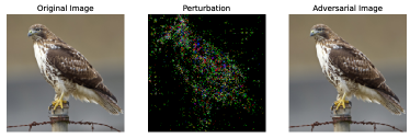
Figure 1: Adversarial examples for ImageNet, as computed by SDF on a ResNet-$50$ (He et al., 2016a) architecture. The original image, which was classified as an ”American eagle” is classified as an ”iguana” by the perturbation vector obtained from SDF.

Our goal in this paper is to introduce a parameter-free and simple method for accurately and reliably evaluating the adversarial robustness of deep networks in a fast and geometrically-based fashion. Most of the current attack methods rely on general-purpose optimization techniques, such as Projected Gradient Descent (PGD) (Madry et al., 2017) and Augmented Lagrangian (Rony et al., 2021), which are oblivious to the geometric properties of models. However, deep neural networks’ robustness to adversarial perturbations is closely tied to their geometric landscape (Dauphin et al., 2014; Poole et al., 2016). Given this, it would be beneficial to exploit such properties when designing and implementing adversarial attacks. This allows to create more effective and computationally efficient attacks on classifiers. Formally, for a given classifier $\hat{k}$, we define an adversarial perturbation as the minimal perturbation $\boldsymbol{r}$ that is sufficient to change the estimated label $\hat{k}(\boldsymbol{x})$:

$$\Delta(\boldsymbol{x};\hat{k}):=\min_{\boldsymbol{r}}\|\boldsymbol{r}\|_{2}\text{ s.t }\hat{k}(\boldsymbol{x}+\boldsymbol{r})\neq\hat{k}(\boldsymbol{x}),$$ (1)

Depending on the data type, $\boldsymbol{x}$ can be any data, and $\hat{k}(\boldsymbol{x})$ is the estimated label.

DeepFool (DF) (Moosavi-Dezfooli et al., 2016) was among the earliest attempts to exploit the “excessive linearity” (Goodfellow et al., 2014) of deep networks to find minimum-norm adversarial perturbations. However, more sophisticated attacks were later developed that could find smaller perturbations at the expense of significantly greater computation time.

In this paper, we exploit the geometric characteristics of minimum-norm adversarial perturbations to design a family of fast yet simple algorithms that become state-of-the-art in finding minimal adversarial perturbation. Our proposed algorithm is based on the geometric principles underlying DeepFool, but incorporates novel enhancements that improve its performance significantly, while maintaining simplicity and efficiency that are only slightly inferior to those of DF. Our main contributions are summarized as follows:

• We introduce a novel family of fast yet accurate algorithms to find minimal adversarial perturbations. We extensively evaluate and compare our algorithms with state-of-the-art attacks in various settings.

• Our algorithms are developed in a systematic and well-grounded manner, based on theoretical analysis.

• We further improve the robustness of state-of-the-art image classifiers to minimum-norm adversarial attacks via adversarial training on the examples obtained by our algorithms.

• We significantly improve the time efficiency of the state-of-the-art Auto-Attack (AA) (Croce & Hein, 2020b) by adding our proposed method to the set of attacks in AA.

Related works. It has been observed that deep neural networks are vulnerable to adversarial examples before in (Szegedy et al., 2013; Carlini & Wagner, 2017; Moosavi-Dezfooli et al., 2016; Goodfellow et al., 2014). The authors in (Szegedy et al., 2013) studied adversarial examples by solving a penalized optimization problems. The optimization approach used in (Szegedy et al., 2013) is complex and computationally inefficient; therefore, it can not scale to large datasets. The method proposed in (Goodfellow et al., 2014) simplify the optimization problem used in (Szegedy et al., 2013) by optimizing it for the $\ell_{\infty}$-norm and relaxing the condition very close to image $\boldsymbol{x}$. DF was the first to attempt to find minimum-norm adversarial perturbations by utilizing an iterative approach that uses a linearization of the classifier at each iteration to estimate the minimal adversarial perturbation. Carlini and Wagner (C$\&$W) (Carlini & Wagner, 2017) transform the optimization problem in (Szegedy et al., 2013) into an unconstrained optimization problem. C$\&$W by leveraging the first-order gradient-based optimizers to minimize a balanced loss between the norm of the perturbation and misclassification confidence. Inspired by the geometrical idea of DF, FAB (Croce & Hein, 2020a) presents an approach to minimize the norm of adversarial perturbations by employing complex projections and approximations while maintaining proximity to the decision boundary. By utilizing gradients to estimate the local geometry of the boundary, this method formulates minimum-norm optimization without the need for tuning a weighting term. FAB cannot be used for large datasets. DDN (Rony et al., 2019) uses projections on the $\ell_{2}$-ball for a given perturbation budget $\epsilon$. FMN (Pintor et al., 2021) extends the DDN attack to other $\ell_{p}$-norms. By formulating (1) with Lagrange’s method, ALMA (Rony et al., 2021) introduced a framework for finding adversarial examples for several distances.

Classifying adversarial attacks help us to understand their core idea. For this reason, we can classify adversarial attacks into two main categories. The first is white-box attacks, and the second is black-box attacks (Chen et al., 2020; Rahmati et al., 2020). In white-box attacks, the attacker knows ”everything”: model architecture, parameters, defending mechanism, etc. In black-box attacks, the attacker has limited knowledge about the model. It can query the model on inputs to observe outputs. In this paper, our focus is on white-box attacks. Formally we can categorize white-box attacks into two sub-categories; the first one is bounded-norm attacks, and the second one is minimum-norm attacks. DeepFool, C$\&$W, FMN, FAB, DDN, and ALMA are minimum-norm attacks, and FGSM, PGD, and momentum extension of PGD (Uesato et al., 2018) are bounded-norm attacks.

The rest of the paper is organized as follows: In Section 2, we introduce minimum-norm adversarial perturbations and characterize their geometrical aspects. Section 3 provides an efficient method for computing $\ell_{2}$ adversarial perturbations by introducing a geometrical solution. Finally, the evaluation and analysis of the computed $\ell_{2}$ perturbations are provided in Section 4.

2 DeepFool (DF) and Minimal Adversarial Perturbations

In this section, we first discuss the geometric interpretation of the minimum-norm adversarial perturbations, i.e., solutions to the optimization problem in (1). We then examine DF to demonstrate why it may fail to find the minimum-norm perturbation. Then in the next section, we introduce our proposed method that exploits DF to find smaller perturbations.

Let $f$ : $\mathbb{R}^{d}\rightarrow\mathbb{R}^{C}$ denote a $C$-class classifier, where $f_{k}$ represents the classifier’s output associated to the $k$th class. Specifically, for a given datapoint $\boldsymbol{x}$ $\in$ $\mathbb{R}^{d}$, the estimated label is obtained by $\hat{k}(\boldsymbol{x})=\text{argmax}_{k}f_{k}(\boldsymbol{x})$, where $f_{k}(\boldsymbol{x})$ is the $k^{\text{th}}$ component of $f(\boldsymbol{x})$ that corresponds to the $k^{\text{th}}$ class.

Note that the classifier $f$ can be seen as a mapping that partitions the input space $\mathbb{R}^{d}$ into classification regions, each of which has a constant estimated label (i.e., $\hat{k}(.)$ is constant for each such region). The decision boundary $\mathscr{B}$ is defined as the set of points in $\mathbb{R}^{d}$ such that $f_{i}(\boldsymbol{x})=f_{j}(\boldsymbol{x})=\max_{k}f_{k}(\boldsymbol{x})$ for some distinct $i$ and $j$.

Additive $\ell_{2}$-norm adversarial perturbations are inherently related to the geometry of the decision boundary. More formally, Let $\boldsymbol{x}\in\mathbb{R}^{d}$, and $\boldsymbol{r}^{*}(\boldsymbol{x})$ be the minimal adversarial perturbation defined as the minimizer of (1). Then $\boldsymbol{r}^{*}(\boldsymbol{x})$, 1) is orthogonal to the decision boundary of the classifier $\mathscr{B}$, and 2) its norm $\|\boldsymbol{r}^{*}(\boldsymbol{x})\|_{2}$ measures the Euclidean distance between $\boldsymbol{x}$ and $\mathscr{B}$, that is $\boldsymbol{x}+\boldsymbol{r}^{*}$ lies on $\mathscr{B}$. We aim to investigate whether the perturbations generated by DF satisfy the aforementioned two conditions. Let $\boldsymbol{r}_{\text{DF}}$ denote the perturbation found by DF for a datapoint $\boldsymbol{x}$. We expect $\boldsymbol{x}+\boldsymbol{r}_{\text{DF}}$ to lie on the decision boundary. Hence, if $\boldsymbol{r}$ is the minimal perturbation, for all $0<\gamma<1$, we expect the perturbation $\gamma\boldsymbol{r}$ to remain in the same decision region as of $\boldsymbol{x}$ and thus fail to fool the model.

In Figure 2, we consider the fooling rate of $\gamma\,\boldsymbol{r}_{\text{DF}}$ for $0.2<\gamma<1$. For a minimum-norm perturbation, we expect an immediate sharp decline for $\gamma$ close to one. However, in Figure 2 we cannot observe such a decline (a sharp decline happens close to $\gamma=0.9$, not 1). This is a confirmation that DF typically finds an overly perturbed point. One potential reason for this is the fact that DF stops when a misclassified point is found, and this point might be an overly perturbed one within the adversarial region, and not necessarily on the decision boundary.

Now, let us consider the other characteristic of the minimal adversarial perturbation. That is, the perturbation should be orthogonal to the decision boundary. We measure the angle between the found perturbation $\boldsymbol{r}_{\text{DF}}$ and the normal vector orthogonal to the decision boundary ($\nabla f(\boldsymbol{x}+\boldsymbol{r}_{\text{DF}})$). To do so, we first scale $\boldsymbol{r}_{\text{DF}}$ such that $\boldsymbol{x}+\gamma\boldsymbol{r}_{\text{DF}}$ lies on the decision boundary. It can be simply done via performing a line search along $\boldsymbol{r}_{\text{DF}}$. We then compute the cosine of the angle between $\boldsymbol{r}_{\text{DF}}$ and the normal to the decision boundary at $\boldsymbol{x}+\gamma\boldsymbol{r}_{\text{DF}}$ (this angle is denoted by $\cos(\alpha)$). For an optimal perturbation, we expect these two vectors to be parallel. In Figure 3, we show the distribution of cosine of this angle. Ideally, we wanted this distribution to be accumulated around one. However, Figure 3 clearly shows that this is not the case, which is a confirmation that $\boldsymbol{r}_{\text{DF}}$ is not necessarily the minimal perturbation.

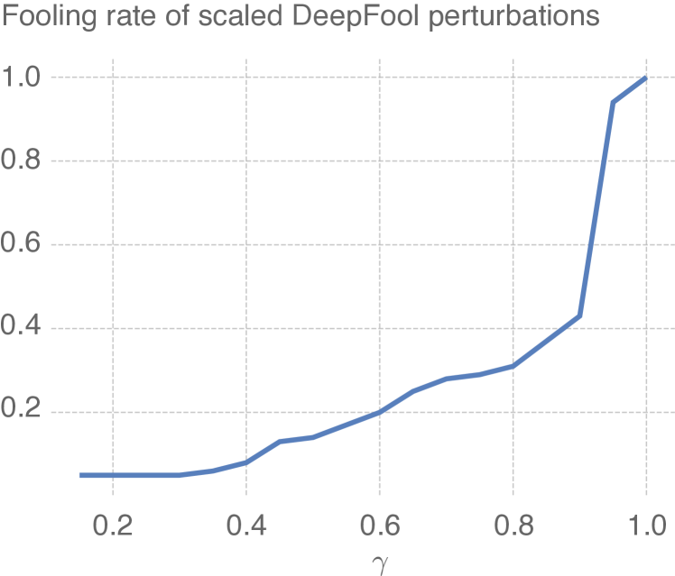
Figure 2: We generated $1000$ images with one hundred $\gamma$ between zero and one, and the fooling rate of the DF is reported. This experiment is done on the CIFAR-$10$ dataset and ResNet-$18$ (He et al., 2016a) model. The accuracy of this Network is $94\%$.

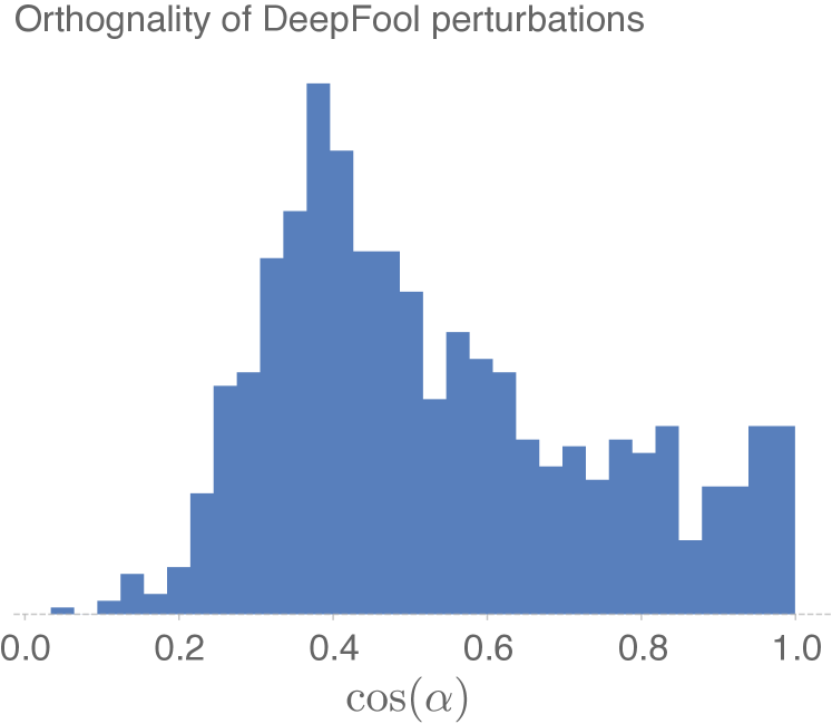
Figure 3: Histogram of the cosine angle distribution between the gradient in the last step of DF and the perturbation vector obtained by DF. This experiment has been performed on $1000$ images from the CIFAR-$10$ (Krizhevsky et al., 2009) dataset with the ResNet-$18$ (He et al., 2016a) model.

3 Efficient Algorithms to Find Minimal Perturbations

In this section, we propose a new class of methods that modifies DF to address the aforementioned challenges in the previous section. The goal is to maintain the desired characteristics of DF, i.e., computational efficiency and the fact that it is parameter-free while finding smaller adversarial perturbations. We achieve this by introducing an additional projection step which its goal is to steer the direction of perturbation towards the optimal solution of (1).

Let us first briefly recall how DF finds an adversarial perturbations for a classifier $f$. Given the current point $\boldsymbol{x}_{i}$, DF updates it according to the following equation:

$${\boldsymbol{x}}_{i+1}=\boldsymbol{x}_{i}-\frac{f(\boldsymbol{x}_{i})}{\|\nabla f(\boldsymbol{x}_{i})\|^{2}_{2}}\nabla f(\boldsymbol{x}_{i}).$$ (2)

Here the gradient is taken w.r.t. the input. The intuition is that, in each iteration, DF finds the minimum perturbation for a linear classifier that approximates the model around $\boldsymbol{x}_{i}$. The below proposition shows that under certain conditions, repeating this update step eventually converges to a point on the decision boundary.

Proposition 1

Let the binary classifier $f:\mathbb{R}^{d}\rightarrow\mathbb{R}$ be continuously differentiable and its gradient $\nabla f$ be $L^{{}^{\prime}}$-Lipschitz. For a given input sample $\boldsymbol{x}_{0}$, suppose $B(\boldsymbol{x}_{0},\epsilon)$ is a ball centered around $\boldsymbol{x}_{0}$ with radius $\epsilon$, such that there exists $\boldsymbol{x}\in B(\boldsymbol{x}_{0},\epsilon)$ that $f(\boldsymbol{x})=0$. If $\|\nabla f\|_{2}\geq\zeta$ for all $\boldsymbol{x}\in B$ and $\epsilon<\frac{\zeta^{2}}{{L^{{}^{\prime}}}^{2}}$, then DF iterations converge to a point on the decision boundary.

Proof: We defer the proof to the Appendix.

Note that while the proposition guarantees the perturbed sample to lie on the decision boundary, it does not state anything about the orthogonality of the perturbation to the decision boundary. Moreover, in practice, DF typically terminates after less than four iterations when an adversarial example is found. As discussed in the previous section, such a solution may not necessarily lie on the decision boundary.

To find perturbations that are more aligned with the normal to the decision boundary, we introduce an additional projection step that steers the perturbation direction towards the optimal solution of (1). Formally, the optimal perturbation, $\boldsymbol{r}^{*}$, and the normal to the decision boundary at $\boldsymbol{x}_{0}+\boldsymbol{r}^{*}$, $\nabla f(\boldsymbol{x}_{0}+\boldsymbol{r}^{*})$, should be parallel. Equivalently, $\boldsymbol{r}^{*}$ should be a solution of the following maximization problem:

$$\max_{\boldsymbol{r}}\frac{{\boldsymbol{r}}^{\top}\nabla f(\boldsymbol{x}_{0}+\boldsymbol{r})}{\|\nabla f(\boldsymbol{x}_{0}+\boldsymbol{r})\|\|\boldsymbol{r}\|},$$ (3)

which is the cosine of the angle between $\boldsymbol{r}$ and $\nabla f(\boldsymbol{x}_{0}+\boldsymbol{r})$. A necessary condition for $\boldsymbol{r}^{*}$ to be a solution of (3) is that the projection of $\boldsymbol{r}^{*}$ on the subspace orthogonal to $\nabla f(\boldsymbol{x}_{0}+\boldsymbol{r}^{*})$ should be zero. Then, $\boldsymbol{r}^{*}$ can be seen as a fixed point of the following iterative map:

$$\boldsymbol{r}_{i+1}=T(\boldsymbol{r}_{i})=\frac{{\boldsymbol{r}_{i}}^{\top}\nabla f(\boldsymbol{x}_{0}+\boldsymbol{r}_{i})}{\|\nabla f(\boldsymbol{x}_{0}+\boldsymbol{r}_{i})\|^{2}}\nabla f(\boldsymbol{x}_{0}+\boldsymbol{r}_{i}).$$ (4)

The following proposition shows that this iterative process can find a solution of (3).

Proposition 2

For a differentiable $f$ and a given $\boldsymbol{r}_{0}$, $\boldsymbol{r}_{i}$ in the iterations (4) either converge to a solution of (3) or a trivial solution (i.e., $\boldsymbol{r}_{i}\rightarrow 0$).

Proof: We defer the proof to the Appendix.

Input: image $\boldsymbol{x}_{0}$, classifier $f$, $m$, and $n$.

Output: perturbation $\boldsymbol{r}$

Initialize: $\boldsymbol{x}\leftarrow\boldsymbol{x}_{0}$

while $\operatorname*{sign}(f(\boldsymbol{x}))=\operatorname*{sign}(f(\boldsymbol{x}_{0}))$ do

       repeat $m$ times

             $\boldsymbol{x}\leftarrow\boldsymbol{x}-\frac{\left|f(\boldsymbol{x})\right|}{\|\nabla f(\boldsymbol{x})\|_{2}^{2}}\nabla f(\boldsymbol{x})$

       end

      repeat $n$ times

             $\boldsymbol{x}\leftarrow\boldsymbol{x}_{0}+\frac{(\boldsymbol{x}-\boldsymbol{x}_{0})^{\top}\nabla f(\boldsymbol{x})}{\|\nabla f(\boldsymbol{x})\|^{2}}\nabla f(\boldsymbol{x})$

       end

      

end while

return $\boldsymbol{r}=\boldsymbol{x}-\boldsymbol{x}_{0}$

Algorithm 1 SDF ($m$,$n$) for binary classifiers

3.1 A Family of Adversarial Attacks

Finding minimum-norm adversarial perturbations can be seen as a multi-objective optimization problem, where we want $f(\boldsymbol{x}+\boldsymbol{r})=0$ and the perturbation $\boldsymbol{r}$ to be orthogonal to the decision boundary. So far we have seen that DF finds a solution satisfying the former objective and the iterative map (4) can be used to find a solution for the latter. A natural approach to satisfy both objectives is to alternate between these two iterative steps, namely (2) and (4). We propose a family of adversarial attack algorithms, coined SuperDeepFool, by varying how frequently we alternate between these two steps. We denote this family of algorithms with SDF$(m,n)$, where $m$ is the number of DF steps (2) followed by $n$ repetition of the projection step (4). This process is summarized in Algorithm 1.

One interesting case is SDF $(\infty,1)$ which, in each iteration, continues DF steps till a point on the decision boundary is found and then applies the projection step. This particular case has a resemblance with the strategy used in (Rahmati et al., 2020) to find black-box adversarial perturbations. This algorithm can be interpreted as iteratively approximating the decision boundary with a hyperplane and then analytically calculating the minimal adversarial perturbation for a linear classifier for which this hyperplane is the decision boundary. It is justified by the observation that the decision boundary of state-of-the-art deep networks has a small mean curvature around data samples (Fawzi et al., 2017, 2018). A geometric illustration of this procedure is shown in Figure 4.

3.2 SDF Attack

We empirically compare the performance of SDF$(m,n)$ for different values of $m$ and $n$ in Section 4.2. Interestingly, we observe that we get better attack performance when we apply several DF steps followed by a single projection. Since the standard DF typically finds an adversarial example in less than four iterations for state-of-the-art image classifiers, one possibility is to continue DF steps till an adversarial example is found and then apply a single projection step. We simply call this particular version of our algorithm SDF, which we will extensively evaluate in Section 4.

SDF can be understood as a generic algorithm that can also work for the multi-class case by simply substituting the first inner loop of Algorithm 1 with the standard multi-class DF algorithm. The label of the obtained adversarial example determines the boundary on which the projection step will be performed. A summary of multi-class SDF is presented in Algorithm 2. Compared to the standard DF, this algorithm has an additional projection step. We will see later that such a simple modification leads to significantly smaller perturbations.

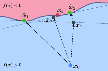
Figure 4: Illustration of two iterations of the SDF($\infty$,1) algorithm. Here $\boldsymbol{x}_{0}$ is the original data point and $\boldsymbol{x}_{*}$ is the minimum-norm adversarial example, that is the closest point on the decision boundary to $\boldsymbol{x}_{0}$. $\tilde{\boldsymbol{x}}_{i}$ and $\boldsymbol{x}_{i}$ indicate the DF and the orthogonal projection steps respectively. The algorithm will eventually converges to $\boldsymbol{x}_{*}$.

Input: image $\boldsymbol{x}_{0}$, classifier $f$.

Output: perturbation $\boldsymbol{r}$

Initialize: $\boldsymbol{x}\leftarrow\boldsymbol{x}_{0}$

while $\hat{k}(\boldsymbol{x})=\hat{k}(\boldsymbol{x}_{0})$ do

       $\widetilde{\boldsymbol{x}}\leftarrow\textnormal{{{DeepFool}}}(\boldsymbol{x})$ $\boldsymbol{w}\leftarrow\nabla f_{\hat{k}(\widetilde{\boldsymbol{x}})}(\widetilde{\boldsymbol{x}})-\nabla f_{\hat{k}(\boldsymbol{x}_{0})}(\widetilde{\boldsymbol{x}})$ $\boldsymbol{x}\leftarrow\boldsymbol{x}_{0}+\frac{(\widetilde{\boldsymbol{x}}-\boldsymbol{x}_{0})^{\top}\boldsymbol{w}}{\|\boldsymbol{w}\|^{2}}\boldsymbol{w}$

end while

return $\boldsymbol{r}=\boldsymbol{x}-\boldsymbol{x}_{0}$

Algorithm 2 SDF for multi-class classifiers

4 Experimental Results

In this section, we conduct extensive experiments to demonstrate the effectiveness of our method in different setups and for several networks. We first introduce our experimental settings, including datasets, models, and attacks. Next, we compare our method with state-of-the-art $\ell_{2}$-norm adversarial attacks in various settings, demonstrating the superiority of our simple yet fast algorithm for finding adversarial examples. Moreover, we add SDF to the collection of attacks used in Auto-Attack (Croce & Hein, 2020b), and call the new set of attacks Auto-Attack++. This setup meaningfully speeds up the process of finding norm-bounded adversarial perturbations. We also demonstrate that a model adversarially training using the SDF perturbations becomes more robust compared to the models trained using other minimum-norm attacks.

4.1 Setup

We test our algorithms on deep convolutional neural network architectures trained on MNIST (LeCun, 1998), CIFAR-10, and ImageNet (Deng et al., 2009) datasets. For the evaluation, we use all the MNIST test dataset, while for CIFAR-10 and ImageNet we use $1000$ samples randomly chosen from their corresponding test datasets. For MNIST, we use a robust model called IBP from (Zhang et al., 2019). For CIFAR-$10$, we use three models: an adversarially trained PreActResNet-$18$ (He et al., 2016b) from (Rade & Moosavi-Dezfooli, 2021), a regularly trained Wide ResNet $28$-$10$ (WRN-$28-10$) from (Zagoruyko & Komodakis, 2016) and LeNet (LeCun et al., 1999). These models are obtainable via the RobustBench library (Croce et al., 2020). On ImageNet, we test the attacks on two ResNet-$50$ (RN-$50$) models: one regularly trained and one $\ell_{2}$ adversarially trained, obtainable through the robustness library (Engstrom et al., 2019).

Table 1: The cosine of the angle between the perturbation vector ($\boldsymbol{r}$) and $\nabla f(\boldsymbol{x}+\boldsymbol{r})$. We performed this experiment on three models trained on CIFAR-$10$ dataset. The evaluation is done using $1000$ random samples.

Attack	Models
	LeNet	ResNet-18	WRN-28-10
DF	$0.89$	$0.14$	$0.21$
SDF (1,1)	$0.90$	$0.63$	$0.64$
SDF (1,3)	$0.88$	$0.61$	$0.62$
SDF (3,1)	$\mathbf{0.92}$	$0.70$	$0.72$
SDF	$\mathbf{0.92}$	$\mathbf{0.72}$	$\mathbf{0.80}$

Table 2: Comparison of the mean and the median of $\ell_{2}$-norm of perturbations for DF and SDF family algorithms. We performed this experiment on CIFAR-$10$. We use the same model architectures and hyperparameters for training as in (Carlini & Wagner, 2017; Rony et al., 2019). For more details about the architecture see the appendix.

Attack	Mean-$\ell_{2}$	Median-$\ell_{2}$	Grads
DF	$0.17$	$0.15$	$\mathbf{14}$
SDF (1,1)	$0.14$	$0.13$	$22$
SDF (1,3)	$0.16$	$0.14$	$26$
SDF (3,1)	$0.12$	$0.11$	$30$
SDF	$\mathbf{0.11}$	$\mathbf{0.10}$	$32$

4.2 Comparison with DeepFool

In this part, we compare our algorithm in terms of orthogonality and size of the $\ell_{2}$-norm perturbations with DF. Assume $\boldsymbol{r}$ is the perturbation vector obtained by an adversarial attack. First, we measure the orthogonality of perturbations by measuring the inner product between $\nabla f(\boldsymbol{x}+\boldsymbol{r})$ and $\boldsymbol{r}$. As we explained in Section 2, a larger inner product between $\boldsymbol{r}$ and the gradient vector at $f(\boldsymbol{x}+\boldsymbol{r})$ indicates that the perturbation vector is closer to the optimal perturbation vector $\boldsymbol{r}^{*}$. We compare the orthogonality of different members of the SDF family and DF for three networks trained on CIFAR-10; namely, LeNet, ResNet-$18$, and WRN-$28$-$10$. The results are shown in Table 1. We observe that DF finds perturbations orthogonal to the decision boundary for low-complexity models such as LeNet, but fails to perform effectively when evaluated against more complex ones. In contrast, attacks from the SDF family consistently found perturbations with a larger cosine of the angle for all three models.

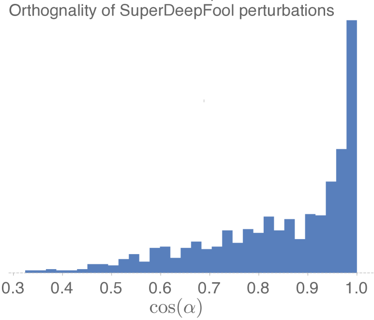
Figure 5: Histogram of the cosine angle distribution between the gradient in the last step of SDF and the perturbation vector obtained by SDF. This experiment has been performed on $1000$ images from the CIFAR-$10$ (Krizhevsky et al., 2009) dataset with the ResNet-$18$ (He et al., 2016a) model.

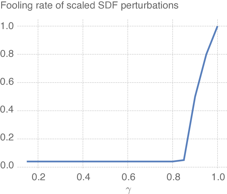
Figure 6: We generated $1000$ images with one hundred $\gamma$ between zero and one, and the fooling rate of the SDF is reported. This experiment is done on the CIFAR-$10$ dataset and ResNet-$18$ model. The accuracy of this network is $94\%$.

Table 2 shows the comparison between the size of the perturbations. These results show that the SDF family finds more accurate perturbations than DF. SDF ($\infty$,1), the strong member of this family, makes a significant difference with DF with little cost.

Comparison with results in Section 2.

We also repeat the experiments we presented for DF in Section 2 for SDF, to show that our method indeed improves the two issues with DF that we highlighted. Namely, the alignment of the perturbation with the normal to the decision boundary and the problem of over-perturbation. In Figure 5, we can see that unlike Figure 3, the cosine of the angle is accumulated around one, which shows that the found perturbation is more aligned with the normal vector to the decision boundary. Moreover, Figure 6 shows a sharp decline in the fooling rate (going down quickly to zero). This is consistent with our expectation for a minimal perturbation attack.

Table 3: Performance for attacks on the MNIST dataset with IBP models. The numbers between parentheses indicate the number of iterations.

Attack	Fooling-rate	Median-$\ell_{2}$	Grads
ALMA ($1000$)	$\mathbf{100}$	$\mathbf{1.26}$	$1\,000$
ALMA ($100$)	$98.90$	$4.96$	$100$
DDN ($1000$)	$99.27$	$1.97$	$1\,000$
DDN ($100$)	$94.34$	$1.46$	$100$
FAB ($1000$)	$99.98$	$3.34$	$10\,000$
FAB ($100$)	$99.98$	$5.19$	$1\,000$
FMN ($1000$)	$89.08$	$1.34$	$1\,000$
FMN ($100$)	$67.80$	$2.14$	$100$
C&W	$4.63$	–	$90\,000$
SDF	$\mathbf{100}$	$1.37$	$\mathbf{52}$

Table 4: Performance for attacks on the CIFAR-$10$ dataset with WRN-$28$-$10$. For see the results on adversarially trained network see Appendix.

Attack	Fooling-rate	Median-$\ell_{2}$	Grads
ALMA	$100$	$0.10$	$100$
DDN	$100$	$0.13$	$100$
FAB	$100$	$0.11$	$100$
FMN	$97.3$	$0.11$	$100$
C&W	$100$	$0.12$	$90\,000$
SDF	$100$	$\mathbf{0.09}$	$\mathbf{25}$

4.3 Comparison with Minimum-Norm Attacks

We now compare our SDF with other minimum $\ell_{2}$-norm state-of-the-art attacks such as C&W, FMN, DDN, ALMA, FAB. For C&W, we use the same hyperparameters as (Carlini & Wagner, 2017; Rony et al., 2019). We use FMN, FAB, DDN, and ALMA with budgets of $100$ and $1000$ iterations and report the best performance. In terms of implementation, we use Pytorch (Paszke et al., 2019). Foolbox (Rauber et al., 2017) and Torchattcks (Kim, 2020) libraries are used to implement adversarial attacks.

We evaluated the robustness of the IBP model, which is adversarially trained on the MNIST dataset, against state-of-the-art attacks in Table 3. SDF and ALMA are the only attacks that achieve a $100\%$ percent fooling rate against the robust model, whereas C&W is unsuccessful on most of the data samples. The fooling rates of the remaining attacks also degrade when evaluated with $100$ iterations. For instance, FMN’s fooling rate decreases from $89\%$ to $67.8\%$ when the number of iterations is reduced from $1000$ to $100$. This observation shows that, unlike SDF, selecting the necessary number of iterations is critical for the success of fixed-iteration attacks. Even for ALMA which can achieve a nearly perfect misclassification rate, decreasing the number of iterations from $1000$ to $100$ causes the median norm of perturbations to increase fourfold. In contrast, SDF is able to compute adversarial perturbations using the fewest number of gradient computations while still outperforming the other algorithms, except ALMA, in terms of the perturbation norm. However, it is worth noting that ALMA requires twenty times more gradient computations compared to SDF to achieve a marginal improvement in the perturbation norm.

Table 4 compares SDF with state-of-the-art attacks on the CIFAR-$10$ dataset. The results show that state-of-the-art attacks have a similar norm of perturbations, but an essential point is the speed of attacks. SDF finds more accurate adversarial perturbation very quickly rather than other algorithms. We also evaluated all attacks on an adversarially trained model for the CIFAR-$10$ dataset. SDF achieves smaller perturbations with half the gradient calculations than other attacks. SDF finds smaller adversarial perturbations for adversarially trained networks at a significantly lower cost than other attacks, requiring only $20\%$ of FAB’s cost and $50\%$ of DDN’s and ALMA’s.

Unlike models trained on CIFAR-$10$, where the attacks typically result in perturbations with similar norm, the differences between attacks are more nuanced for ImageNet models. In particular, attacks such as FAB, DDN, and FMN lose their accuracy when the dataset changes. In contrast, SDF achieves smaller perturbations at a significantly lower cost than ALMA. This shows that the geometric interpretation of optimal adversarial perturbation, rather than viewing (1) as a non-convex optimization problem, can lead to an efficient solution. On the complexity aspect, the proposed approach is substantially faster than the other methods. In contrast, these approaches involve a costly minimization of a series of objective functions. We empirically observed that SDF converges in less than $5$ or $6$ iterations to a fooling perturbation; our observations show that SDF consistently achieves state-of-the-art minimum-norm perturbations across different datasets, models, and training strategies, while requiring the least number of gradient computations. This makes it readily suitable to be used as a baseline method to estimate the robustness of very deep neural networks on large datasets.

Table 5: The performance comparison of SDF with other state-of-the-art attacks for median $\ell_{2}$ on ImageNet dataset. FR columns show the fooling rates of attacks.

Model	Attack	FR	Median-$\ell_{2}$	Grads
RN-$50$	ALMA	$\mathbf{100}$	$0.10$	$100$
	DDN	$99.9$	$0.17$	$1\,000$
	FAB	$99.3$	$0.10$	$900$
	FMN	$99.3$	$0.10$	$1\,000$
	C&W	$\mathbf{100}$	$0.21$	$82\,667$
	SDF	$\mathbf{100}$	$\mathbf{0.09}$	$\mathbf{37}$
RN-$50$ (AT)	ALMA	$\mathbf{100}$	$0.85$	$100$
	DDN	$99.7$	$1.10$	$1\,000$
	FAB	$\mathbf{100}$	$0.81$	$900$
	FMN	$99.9$	$0.82$	$1\,000$
	C&W	$99.9$	$1.17$	$52\,000$
	SDF	$\mathbf{100}$	$\mathbf{0.80}$	$\mathbf{49}$

4.4 SDF Adversarial Training (AT)

In this section, we evaluate the performance of a model adversarially trained using SDF against minimum-norm attacks and AutoAttack (Croce & Hein, 2020b). Our experiments provide valuable insights into the effectiveness of adversarial training with SDF and sheds light on its potential applications in building more robust models.

Adversarial training has become a powerful approach to fortify deep neural networks against adversarial perturbations. However, some adversarial attacks, such as C$\&$W, pose a challenge due to their high computational cost and complexity, making them unsuitable for adversarial training. Therefore, an attack that is parallelizable on batch size and gradient computation is necessary for successful adversarial training. SDF possesses these crucial properties, making it a promising candidate for building more robust models.

We adversarially train a WRN-$28$-$10$ on CIFAR-$10$. Similar to the procedure followed in (Rony et al., 2019), we restrict $\ell_{2}$-norms of perturbation to $2.6$ and set the maximum number of iterations for SDF to $6$. We train the model on clean examples for the first $200$ epochs, and we then fine-tune it with SDF generated adversarial examples for $60$ more epochs. Our model reaches a test accuracy of $90.8\%$ while the model by (Rony et al., 2019) obtains $89.0\%$. In (Rony et al., 2019), vanilla adversarial training with DDN generated adversarial examples is shown build a more robust model than a model trained with PGD (Madry et al., 2017). For this reason, we compare our model with (Rony et al., 2019). SDF adversarially trained model does not overfit to SDF attack because, as Table 6 shows, SDF obtains the smallest perturbation. It is evident that SDF adversarially trained model can significantly improve the robustness of model against minimum-norm attacks up to $30\%$. In terms of comparison of these two adversarially trained models with Auto Attack (AA) (Croce & Hein, 2020b), our model outperformed the (Rony et al., 2019) by improving about $8.4\%$ against $\ell_{\infty}$-AA, for $\varepsilon=8/255$, and $0.6\%$ against $\ell_{2}$-AA, for $\varepsilon=0.5$.

Table 6: The comparison between $\ell_{2}$ robustness of our adversarial trained model and (Rony et al., 2019) model. We perform this experiment on $1000$ samples from CIFAR-$10$ dataset. Gain is calculated as a percentage of the difference between the medians. The gain column shows the amount of gain that our model obtains.

Attack	SDF (Ours)		DDN
	Mean	Median	Mean	Median	Gain
DDN	$1.09$	$1.02$	$0.86$	$0.73$	$\uparrow$$29\%$
FAB	$1.12$	$1.03$	$0.92$	$0.75$	$\uparrow$$28\%$
FMN	$1.48$	$1.43$	$1.47$	$1.43$	$0\%$
ALMA	$1.17$	$1.06$	$0.84$	$\mathbf{0.71}$	$\uparrow$$35\%$
SDF	$\mathbf{1.06}$	$\mathbf{1.01}$	$\mathbf{0.81}$	$0.73$	$\uparrow$$28\%$

Furthermore, compared to a network trained on DDN samples, our adversarially trained model has a smaller input curvature (Table 7). This observation corroborates the idea that a more robust network will exhibit a smaller input curvature (Moosavi-Dezfooli et al., 2019; Srinivas et al., ; Qin et al., 2019).

Table 7: The average input curvature of WRN-$28$-$10$ models trained on CIFAR-$10$ dataset, according to the measures proposed in (Srinivas et al., ). The second column shows the average spectral-norm of the Hessian w.r.t. input, $\|\nabla^{2}f(\boldsymbol{x})\|_{2}$, and the third column shows the average of the same quantity normalized by the norm of the input gradient, $\mathcal{C}_{f}(\boldsymbol{x})=\|\nabla^{2}f(\boldsymbol{x})\|_{2}/\|\nabla f(\boldsymbol{x})\|_{2}$.

Model	$\mathbb{E}_{\boldsymbol{x}}\|\nabla^{2}f(\boldsymbol{x})\|_{2}$	$\mathbb{E}_{\boldsymbol{x}}\mathcal{C}_{f}(\boldsymbol{x})$
Standard	$600.06$ $\pm$ $29.76$	$73.99$ $\pm$ $6.62$
DDN AT	$2.86$ $\pm$ $1.22$	$4.32$ $\pm$ $2.91$
SDF AT (Ours)	$\mathbf{0.73}$ $\pm$ $0.08$	$\mathbf{1.66}$ $\pm$ $0.86$

4.5 AutoAttack++

Table 8: An analysis of robust accuracy ($\%$) for various defense strategies against AA++ and AA with $\varepsilon=0.5$. The ”acc” column denotes the robust accuracies of different models. R1 (Rebuffi et al., 2021), R2 (Sehwag et al., 2021), R3 (Gowal et al., 2020) and R4 (Rice et al., 2020) have been trained adversarially, and model S (Zagoruyko & Komodakis, 2016) is a regularly trained model. All models are taken from the RobustBench library (Croce et al., 2020).

Models	Clean	AA		AA++
	acc	acc	Grads	acc	Grads
R1	$95.7\%$	$82.3\%$	$1259.2$	$\mathbf{82.1\%}$	$\mathbf{599.5}$
R2	$90.3\%$	$76.1\%$	$1469.1$	$76.1\%$	$\mathbf{667.7}$
R3	$89.4\%$	$63.4\%$	$1240.4$	$\mathbf{62.2\%}$	$\mathbf{431.5}$
R4	$88.6\%$	$\mathbf{67.6\%}$	$933.7$	$68.4\%$	$\mathbf{715.3}$
S	$94.7\%$	$0.00\%$	$208.6$	$0.00$	$\mathbf{121.1}$

In this part, we introduce a new variant of AutoAttack (Croce & Hein, 2020b) by introducing AutoAttack++ (AA++). Auto-Attack (AA) is a reliable and powerful ensemble attack that contains three types of white-box and a strong black-box attacks. AA evaluates the robustness of a trained model to adversarial perturbations whose $\ell_{2}$/$\ell_{\infty}$-norm is bounded by $\varepsilon$. By substituting SDF with the attacks in the AA, we significantly increase the performance of AA in terms of computational time. Since SDF is an $\ell_{2}$-norm attack, we use the $\ell_{2}$-norm version of AA as well. We restrict maximum iterations of SDF to $10$. If the norm of perturbations exceeds $\varepsilon$, we renormalize the perturbation to ensure its norm stays $\leq\varepsilon$. In this context, we have modified the AA algorithm by replacing APGD^⊤ (Croce & Hein, 2020b) with SDF due to the former’s cost and computation bottleneck in the context of AA. We compare the fooling rate and computational time of AA++ and AA on the stat-of-the-art models from the RobustBench (Croce et al., 2020) leaderboard. In Table 8, we observe that AA++ is up to three times faster than AA. In an alternative scenario, we added the SDF to the beginning of the AA set, resulting in a version that is up to two times faster than the original AA, despite now containing five attacks (see Appendix). This outcome highlights the efficacy of SDF in finding adversarial examples. These experiments suggest that leveraging efficient minimum-norm and non-fixed iteration attacks, such as SDF, can enable faster and more reliable evaluation of the robustness of deep models.

5 Conclusion

In this work, we have introduced a family of parameter-free, fast, and parallelizable algorithms for crafting optimal adversarial perturbations. Our proposed algorithm, SuperDeepFool, outperforms state-of-the-art $\ell_{2}$-norm attacks, while maintaining a small computational cost. We have demonstrated the effectiveness of SuperDeepFool in various scenarios. Furthermore, we have shown that adversarial training using the examples generated by SuperDeepFool builds more robust models. For future work, one potential avenue could be to extend SuperDeepFool families to other threat models, such as general $\ell_{p}$-norms.

6 Acknowledgments

We want to thank Kosar Behnia and Mohammad Azizmalayeri for their helpful feedback. We are very grateful to Fabio Brau and Jérôme Rony for providing code and models and answering questions on their papers.

7 Proofs

Proof of Proposition 1.

Since $\nabla f(\boldsymbol{x})$ is Lipschitz-continuous, for $\boldsymbol{x},\boldsymbol{y}\in B(\boldsymbol{x}_{0},\epsilon)$, we have:

$$|f(\boldsymbol{x})-f(\boldsymbol{y})+\nabla f(\boldsymbol{y})^{T}(\boldsymbol{x}-\boldsymbol{y})|\leq\frac{L^{{}^{\prime}}}{2}\|\boldsymbol{x}-\boldsymbol{y}\|^{2}$$ (5)

DeepFool updates the new $\boldsymbol{x}_{n}$ in each according to the following equation:

$$\boldsymbol{x}_{n}=\boldsymbol{x}_{n-1}+\frac{\nabla f(\boldsymbol{x}_{n-1})}{\|\nabla f(\boldsymbol{x}_{n-1})\|_{2}}f(\boldsymbol{x}_{n-1})$$ (6)

Hence if we substitute $\boldsymbol{x}=\boldsymbol{x}_{n}$ and $\boldsymbol{y}=\boldsymbol{x}_{n-1}$ in 5, we get:

$$|f(\boldsymbol{x}_{n})|\leq\frac{L^{{}^{\prime}}}{2}\|\boldsymbol{x}_{n}-\boldsymbol{x}_{n-1}\|^{2}.$$ (7)

Now, let $s_{n}:=||\boldsymbol{x}_{n}-\boldsymbol{x}_{n-1}||$. Using 7 and DeepFool’s step, we get:

$$s_{n+1}=\frac{f(\boldsymbol{x}_{n})}{\|\nabla f(\boldsymbol{x}_{n})\|}\leq\frac{L^{{}^{\prime}}}{2\zeta}\frac{f(\boldsymbol{x}_{n})^{2}}{\|\nabla f(\boldsymbol{x}_{n})\|^{2}}$$ (8)

We also know that for $\boldsymbol{x},\boldsymbol{x}^{*}\in B(\boldsymbol{x}_{0},\epsilon)$ and the Lipschitz property:

$$|f(\boldsymbol{x})-f(\boldsymbol{x}^{*})|\leq 2L^{{}^{\prime}}\epsilon$$ (9)

From property $\boldsymbol{x}^{*}$ we know that $f(\boldsymbol{x}^{*})=0$, so:

$$|f(\boldsymbol{x})|\leq 2L^{{}^{\prime}}\epsilon$$ (10)

$$s_{n+1}=\frac{f(\boldsymbol{x}_{n})}{||\nabla f(\boldsymbol{x}_{n})||}\leqslant s_{n}\epsilon\frac{L^{{}^{\prime}2}}{\zeta^{2}}$$ (11)

Using the assumptions of the theorem, We have $\frac{L^{{}^{\prime}}\epsilon}{\zeta^{2}}<1$,  and hence $s_{n}$ converges to $0$ when $n\rightarrow\infty$.  We conclude that $\{\boldsymbol{x}_{n}\}$ is a Cauchy sequence. Denote by $\boldsymbol{x}_{\infty}$ the limit point of $\{\boldsymbol{x}_{n}\}$. Using the continuity of $f$ and Eq.(7),  we obtain

$$\lim_{n\rightarrow\infty}|f(\boldsymbol{x}_{n})|=|f(\boldsymbol{x}_{\infty})|=|f(\boldsymbol{x}^{*})|=0,$$ (12)

It is clear that $\boldsymbol{x}^{*}$ is $\boldsymbol{x}$. which concludes the proof of the theorem.

Proof of Proposition 2. Let us denote the acute angle between $\nabla f(\boldsymbol{x}_{0}+\boldsymbol{r}_{i})$ and $\boldsymbol{r}_{i}$ by $\theta_{i}$ ($0\leq\theta_{i}\leq\pi/2$). Then from (4) we have $|\boldsymbol{r}_{i+1}|=|\boldsymbol{r}_{i}|\cos\theta_{i}$. Therefore, we get

$$|\boldsymbol{r}_{i+1}|=\prod_{i=1}^{i}\cos\theta_{i}|\boldsymbol{r}_{0}|.$$ (13)

Now there are two cases, either $\theta_{i}\to 0$ or not. Let us first consider the case where zero is not the limit of $\theta_{i}$. Then there exists some $\epsilon_{0}>0$ such that for any integer $N$ there exists some $n>N$ for which we have $\theta_{n}>\epsilon_{0}$. Now for $\epsilon_{0}$, we can have a series of integers $n_{i}$ where for all of them we have $\theta_{n_{i}}>\epsilon_{0}$. Since we have $0\leq|\cos\theta|\leq 1$, we have the following inequality:

$$0\leq\prod_{i=0}^{\infty}|\cos\theta_{i}|\leq\prod_{i=0}^{\infty}|\cos\theta_{n_{i}}|\leq\prod_{i=0}^{\infty}|\cos\epsilon_{0}|$$ (14)

The RHS of the above inequality goes to zero which proves that $\boldsymbol{r}_{i}\to 0$. This leaves us with the other case where $\theta_{i}\to 0$. This means that $\cos\theta_{i}\to 1$ which is the maximum of (3), this completes the proof.

8 On the benefits of line search

As we show in Figure 2 DF typically finds an overly perturbed point. SDF’s gradients depend on DF, so overly perturbing DF is problematic. Line search is a mechanism that we add to the end of our algorithms to tackle this problem. For a fair comparison between adversarial attacks, we add this algorithm to the end of other algorithms to investigate the effectiveness of line search.

Table 9: Comparison of the effectiveness of line search on the CIFAR-$10$ data for SDF and DF. We use one regularly trained model S (WRN-$28$-$10$) and three adversarially trained models (shown with R1 (Rony et al., 2019), R2 (Augustin et al., 2020) and R3 (Rade & Moosavi-Dezfooli, 2021)). ✓and ✗ indicate the presence and absence of line search respectively.

Model	DF		SDF
	✓	✗	✓	✗
S	$0.16$	$0.19$	$\mathbf{0.09}$	$0.10$
R1	$0.87$	$1.02$	$\mathbf{0.73}$	$0.76$
R2	$1.40$	$1.73$	$\mathbf{0.91}$	$0.93$
R3	$1.13$	$1.36$	$\mathbf{1.04}$	$1.09$

As shown in Table 9, we observe that line search can increase the performance of the DF significantly. However, this effectiveness for SDF is a little.

We now measure the effectiveness of line search for other attacks. As observed from Table 10, line search effectiveness for DDN and ALMA is small.

Table 10: Comparison of the effectiveness of line search on the CIFAR-10 data for other attacks. Line search effects are a little for DDN and ALMA. For FMN and FAB because they use line search at the end of their algorithms (they remind this algorithm as a binary search and final search, respectively), line search does not become effective.

Model	DDN		ALMA		FMN		FAB
	✓	✗	✓	✗	✓	✗	✓	✗
WRN-$28$-$10$	$0.12$	$0.13$	$0.10$	$0.10$	$0.11$	$0.11$	$0.11$	$0.11$
R1 (Rony et al., 2019)	$0.73$	$0.73$	$0.71$	$0.71$	$1.10$	$1.10$	$0.75$	$0.75$
R2 (Augustin et al., 2020)	$0.96$	$0.97$	$0.93$	$0.94$	$0.95$	$0.95$	$1.03$	$1.03$
R3 (Rade & Moosavi-Dezfooli, 2021)	$1.04$	$1.04$	$1.06$	$1.06$	$1.08$	$1.08$	$1.07$	$1.07$

9 Comparison on CIFAR-$10$ with the PRN-$18$

In this section, we compare SDF with other minimum-norm attacks against an adversarially trained network (Rade & Moosavi-Dezfooli, 2021). In Table 11, SDF achieves smaller perturbation compared to other attacks, whereas it costs only half as much as other attacks.

Table 11: Comparison of SDF with other state-of-the-art attacks for median $\ell_{2}$ on CIFAR-$10$ dataset for adversarially trained network (PRN-$18$ (Rade & Moosavi-Dezfooli, 2021)).

Attack	FR	Median-$\ell_{2}$	Grads
ALMA	$100$	$0.68$	$100$
DDN	$100$	$0.73$	$100$
FAB	$100$	$0.77$	$210$
FMN	$99.7$	$0.81$	$100$
SDF	$100$	$\mathbf{0.65}$	$\mathbf{46}$

10 Performance comparison of adversarially trained models versus Auto-Attack (AA)

Evaluating the adversarially trained models with attacks used in the training process is not a standard evaluation in the robustness literature. For this reason, we evaluate robust models with AA. We perform this experiment with two modes; first, we measure the robustness of models with $\ell_{\infty}$ norm, and in a second mode, we evaluate them in terms of $\ell_{2}$ norm. Tables 12 and 13 show that adversarial training with SDF samples is more robust against reliable AA than the model trained on DDN samples (Rony et al., 2019).

Table 12: Robustness results of adversarially trained models on CIFAR-$10$ with $\ell_{\infty}$-AA. We perform this experiment on $1000$ samples for each $\epsilon$.

Model	Natural	$\varepsilon=\frac{6}{255}$	$\frac{8}{255}$	$\frac{10}{255}$
DDN	$89.1$	$45$	$29.6$	$17.6$
SDF (Ours)	$90.8$	$\mathbf{47.5}$	$\mathbf{38.1}$	$\mathbf{25.4}$

Table 13: Robustness results of adversarially trained models on CIFAR-$10$ with $\ell_{2}$-AA. We perform this experiment on $1000$ samples for each $\epsilon$.

Model	Natural	$\varepsilon=0.3$	$0.4$	$0.5$	$0.6$
DDN	$89.1$	$78.1$	$73$	$67.5$	$61.7$
SDF (Ours)	$90.8$	$\mathbf{83.1}$	$\mathbf{79.7}$	$\mathbf{68.1}$	$\mathbf{63.9}$

11 Another variants of AA++

As we mentioned, in an alternative scenario, we added the SDF to the beginning of the AA set, resulting in a version that is up to two times faster than the original AA. In this scenario, we do not exchange the SDF with APGD. We add SDF to the AA configuration. So in this configuration, AA has five attacks (SDF, APGD, APGD^⊤, FAB, Square). By this design, we guarantee the performance of AA. An interesting phenomenon observed from these tables is that when the budget increases, the speed of the AA++ increases. We should note that we restrict the number of iterations for SDF to $10$.

(a) R1

(b) S

Figure 7: In this figure, we show the time ratio of AA to AA++. For regularly trained model (WRN-$28$-$10$) and adversarially trained model (Rade & Moosavi-Dezfooli, 2021) (R1). We perform this experiment on $1000$ samples from CIFAR-$10$ data.

12 Why do we need stronger minimum-norm attacks?

Bounded-norm attacks like FGSM (Goodfellow et al., 2014), PGD (Madry et al., 2017), and momentum variants of PGD (Uesato et al., 2018), by optimizing the difference between the logits of the true class and the best non-true class, try to find an adversarial region with maximum confidence within a given, fixed perturbation size. Bounded-norm attacks only evaluate the robustness of deep neural networks; this means that they report a single scalar value as robust accuracy for a fixed budget. The superiority of minimum-norm attacks is to report a distribution of perturbation norms, and they do not report a percentage of fooling rates (robust accuracy) by a single scalar value. This critical property of minimum-norm attacks helps to accelerate to take an in-depth intuition about the geometrical behavior of deep neural networks.

We aim to address a phenomenon we observe by using the superiority of minimum-norm attacks. We observed that a minor change within the design of deep neural networks affects the performance of adversarial attacks. To show the superiority of minimum-norm attacks, we show how minimum-norm attacks verify these minor changes rather than bounded-norm attacks.

Modeling with max-pooling was a fundamental aspect of convolutional neural networks when they were first introduced as the best image classifiers. Some state-of-the-art classifiers such as (Krizhevsky et al., 2017; Simonyan & Zisserman, 2014; He et al., 2016a) use this layer in network configuration. We use the pooling layers to show that using the max-pooling and Lp-pooling layer in the network design leads to finding perturbation with a bigger $\ell_{2}$-norm.

Assume that we have a classifier ($f$). We train $f$ in two modes until the training loss converges. In the first mode, $f$ is trained in the presence of the pooling layer in its configuration, and in the second mode, $f$ does not have a pooling layer. When we measure the robustness of these two networks with regular budgets used in bounded-norms attacks like PGD ($\varepsilon=8/255$), we observe that the robust accuracy is equal to $0\%$. This is precisely where bounded-norm attacks such as PGD mislead robustness literature in its assumptions regarding deep neural network properties. However, a solution to solve the problem of bounded-norm attack scan be proposed: ” Analyzing the quantity of changes in robust accuracy across different epsilons reveal these minor changes.” Is this case, the solution is costly. This is precisely where the distributive view of perturbations from worst-case to best-case of minimum-norm attacks detects this minor change.

To show these changes, we trained ResNet-$18$ (RN-$18$) and Mobile-Net (Howard et al., 2017) in two settings. In the first setting, we trained them in the presence of a pooling layer until the training loss converged, and in the second setting, we trained them in the absence of a pooling layer until the training loss converged. We should note that we remove all pooling-layers in these two settings. For a fair comparison, we train models until they achieve zero training loss using a multi-step learning rate. We use max-pooling and Lp-pooling, for $p=2$, for this minor changes.

Table 14 shows that using a pooling layer in network configuration can increase robustness. DF has an entirely different behavior according to the presence or absence of the pooling layer; max-pooling affects up to $50\%$ of DF performance. This effect is up to $9\%$ for DDN and FMN. ALMA and SDF show a $4\%$ impact in their performance, which shows their consistency compared to other attacks.

Table 14: This table shows the $\ell_{2}$-median for the minimum-norm attacks. For all networks, we set learning rate = $0.01$ and weight decay = $0.01$. For training with Lp-pooling, we set $p=2$ for all settings.

Attack	ResNet-$18$			MobileNet
	no pooling	max-pooling	Lp-pooling	no pooling	max-pooling	Lp-pooling
DF	$0.40$	$0.90$	$0.91$	$0.51$	$0.95$	$0.93$
DDN	$0.16$	$0.25$	$0.26$	$0.22$	$0.27$	$0.26$
FMN	$0.18$	$0.27$	$0.30$	$0.24$	$0.30$	$0.29$
C$\&$W	$0.18$	$0.25$	$0.27$	$0.22$	$0.26$	$0.24$
ALMA	$0.19$	$0.23$	$0.23$	$\mathbf{0.20}$	$0.25$	$0.22$
SDF	$\mathbf{0.16}$	$\mathbf{0.21}$	$\mathbf{0.22}$	$\mathbf{0.20}$	$\mathbf{0.23}$	$\mathbf{0.21}$

As shown in Table 15, we observe that models with pooling-layers have more robust accuracy when facing adversarial attacks such as AA and PGD. It should be noted that using regular epsilon for AA and PGD will not demonstrate these modifications. For this reason, we choose an epsilon for AA and PGD lower ($\varepsilon=2/255$) than the regular format ($\varepsilon=8/255$).

Table 15: This table shows the robust accuracy for all networks against to the AA and PGD. For training with Lp-pooling, we set $p=2$ for all settings.

Attack	ResNet-$18$			MobileNet
	no pooling	max-pooling	Lp-pooling	no pooling	max-pooling	Lp-pooling
AA	$1.1\%$	$17.2\%$	$16.3\%$	$8.7\%$	$21.3\%$	$20.2\%$
PGD	$9.3\%$	$28\%$	$26.2\%$	$16.8\%$	$31.4\%$	$28.7\%$

Table 14 and 15 demonstrate that including pooling-layers can enhance the ability of the neural network to withstand various types of adversarial attacks. Powerful attacks such as SDF and ALMA show high consistency in these setup modifications, highlighting the need for powerful attacks.

12.1 Analysis of max-pooling from the perspective of curvature and Hessian norms.

Here, we take a step further and investigate why max-pooling impacts the robustness of models. In order to perform this analysis, we analyze gradient norms, Hessian norms, and the model’s curvature. The curvature of a point is a mathematical quantity that indicates the degree of nonlinearity. A function’s curvature is often expressed as the norm of the Hessian at a particular point (Moosavi-Dezfooli et al., 2019). Mainly, robust models are characterized by low gradient norms (Hein & Andriushchenko, 2017), implying smaller Hessian norms. In order to investigate robustness independent of non-linearity, (Srinivas et al., ) propose normalized curvature, which normalizes the Hessian norm by its corresponding gradient norm. They defined normalized curvature for a neural network classifier $f$ as $\mathcal{C}_{f}(\boldsymbol{x})=\|\nabla^{2}f(\boldsymbol{x})\|_{2}/(\|\nabla f(\boldsymbol{x})\|_{2}+\varepsilon)$. Where $\|\nabla f(\boldsymbol{x})\|_{2}$ and $\|\nabla^{2}f(\boldsymbol{x})\|_{2}$ are the $\ell_{2}$-norm of the gradient and the spectral norm of the Hessian, respectively, where $\nabla f(\boldsymbol{x})\in\mathbb{R}^{d},\nabla^{2}f(\boldsymbol{x})\in\mathbb{R}^{d\times d}$, and $\varepsilon>0$ is a small constant to ensure the proper behavior of the measure. We use this metric to conduct our experiments.

Table 16: Model geometry of different ResNet-$18$ models. W (with pooling) and W/O (without pooling).

Model	$\mathbb{E}_{\boldsymbol{x}}\|\nabla f(\boldsymbol{x})\|_{2}$	$\mathbb{E}_{\boldsymbol{x}}\|\nabla^{2}f(\boldsymbol{x})\|_{2}$	$\mathbb{E}_{\boldsymbol{x}}\mathcal{C}_{f}(\boldsymbol{x})$
w	$\mathbf{4.75}$ $\pm$ $1.54$	$\mathbf{120.70}$ $\pm$ $48.74$	$\mathbf{14.94}$ $\pm$ $0.52$
w/o	$7.04$ $\pm$ $2.44$	$269.74$ $\pm$ $10.23$	$22.81$ $\pm$ $2.58$

Table 17: Model geometry for regular and adversarially trained models.

Model	$\mathbb{E}_{\boldsymbol{x}}\|\nabla f(\boldsymbol{x})\|_{2}$	$\mathbb{E}_{\boldsymbol{x}}\|\nabla^{2}f(\boldsymbol{x})\|_{2}$	$\mathbb{E}_{\boldsymbol{x}}\mathcal{C}_{f}(\boldsymbol{x})$
Standard	$9.54$ $\pm$ $1.02$	$600.06$ $\pm$ $29.76$	$73.99$ $\pm$ $6.62$
DDN AT	$0.91$ $\pm$ $0.34$	$2.86$ $\pm$ $1.22$	$4.32$ $\pm$ $2.91$
SDF AT	$\mathbf{0.38}$ $\pm$ $0.60$	$\mathbf{0.73}$ $\pm$ $0.08$	$\mathbf{1.66}$ $\pm$ $0.86$

13 CNN architecture used for the CIFAR-$10$ in one scenario

Table 18 shows layers used in (Carlini & Wagner, 2017) and (Rony et al., 2019) for evaluation on CIFAR-$10$.

Layer Type	CIFAR-$10$
Convolution + ReLU	$3\times 3\times 64$
Convolution + ReLU	$3\times 3\times 64$
max-pooling	$2\times 2$
Convolution + ReLU	$3\times 3\times 128$
Convolution + ReLU	$3\times 3\times 128$
max-pooling	$2\times 2$
Fully Connected + ReLU	$256$
Fully Connected + ReLU	$256$
Fully Connected + Softmax	$10$

Table 18: CNN architecture.

14 Multi class algorithms for SDF(1,3) and SDF(1,1)

We have introduced how to generate adversarial examples with the SDF algorithm in the main body of this paper. This section gives more details about combining SDF steps for multi-class settings. We provide the pseudo-code of SDF(1,1) and SDF(1,3) in Algorithm 3 and 4.

Input: image $\boldsymbol{x}$, classifier $f$.

Output: perturbation $\boldsymbol{r}$

Initialize: $\boldsymbol{x}_{0}\leftarrow\boldsymbol{x},\enskip i\leftarrow 0$

while $\hat{k}(\boldsymbol{x}_{i})=\hat{k}(\boldsymbol{x}_{0})$ do

       for $k\neq\hat{k}(\boldsymbol{x}_{0})$ do

             $\boldsymbol{w}^{\prime}_{k}\leftarrow\nabla f_{k}(\boldsymbol{x}_{i})-\nabla f_{\hat{k}(\boldsymbol{x}_{0})}(\boldsymbol{x}_{i})$ $f^{\prime}_{k}\leftarrow f_{k}(\boldsymbol{x}_{i})-f_{\hat{k}(\boldsymbol{x}_{0})}(\boldsymbol{x}_{i})$

       end for

      $\hat{l}\leftarrow\operatorname*{arg\,min}_{k\neq{\hat{k}(\boldsymbol{x}_{0})}}\frac{\left|f^{\prime}_{k}\right|}{\|\boldsymbol{w}^{\prime}_{k}\|_{2}}$ $\boldsymbol{\widetilde{r}}\leftarrow\frac{\left|f^{\prime}_{\hat{l}}\right|}{\|\boldsymbol{w}^{\prime}_{\hat{l}}\|_{2}^{2}}\boldsymbol{w}^{\prime}_{\hat{l}}$ $\widetilde{\boldsymbol{x}}_{i}=\boldsymbol{x}_{i}+\boldsymbol{\widetilde{r}}$ $\boldsymbol{w}_{i}\leftarrow\nabla f_{k(\widetilde{\boldsymbol{x}}_{i})}(\widetilde{\boldsymbol{x}}_{i})-\nabla f_{k(\boldsymbol{x}_{0})}(\widetilde{\boldsymbol{x}}_{i})$ $\boldsymbol{x}\leftarrow\boldsymbol{x}_{0}+\frac{(\widetilde{\boldsymbol{x}}_{i}-\boldsymbol{x}_{0})^{\top}\boldsymbol{w}_{i}}{\|\boldsymbol{w}_{i}\|^{2}}\boldsymbol{w}_{i}$ $i\leftarrow i+1$

end while

return $\boldsymbol{r}=\boldsymbol{x}_{i}-\boldsymbol{x}_{0}$

Algorithm 3 SDF ($1$,$1$)

Input: image $\boldsymbol{x}$, classifier $f$.

Output: perturbation $\boldsymbol{r}$

Initialize: $\boldsymbol{x}_{0}\leftarrow\boldsymbol{x},\enskip i\leftarrow 0$

while $\hat{k}(\boldsymbol{x}_{i})=\hat{k}(\boldsymbol{x}_{0})$ do

       for $k\neq\hat{k}(\boldsymbol{x}_{0})$ do

             $\boldsymbol{w}^{\prime}_{k}\leftarrow\nabla f_{k}(\boldsymbol{x}_{i})-\nabla f_{\hat{k}(\boldsymbol{x}_{0})}(\boldsymbol{x}_{i})$ $f^{\prime}_{k}\leftarrow f_{k}(\boldsymbol{x}_{i})-f_{\hat{k}(\boldsymbol{x}_{0})}(\boldsymbol{x}_{i})$

       end for

      $\hat{l}\leftarrow\operatorname*{arg\,min}_{k\neq{\hat{k}(\boldsymbol{x}_{0})}}\frac{\left|f^{\prime}_{k}\right|}{\|\boldsymbol{w}^{\prime}_{k}\|_{2}}$ $\boldsymbol{\widetilde{r}}\leftarrow\frac{\left|f^{\prime}_{\hat{l}}\right|}{\|\boldsymbol{w}^{\prime}_{\hat{l}}\|_{2}^{2}}\boldsymbol{w}^{\prime}_{\hat{l}}$ $\widetilde{\boldsymbol{x}}_{i}=\boldsymbol{x}_{i}+\boldsymbol{\widetilde{r}}$ for $3$ steps do

             $\boldsymbol{w}_{i}\leftarrow\nabla f_{k(\widetilde{\boldsymbol{x}}_{i})}(\widetilde{\boldsymbol{x}}_{i})-\nabla f_{k(\boldsymbol{x}_{0})}(\widetilde{\boldsymbol{x}}_{i})$ $\boldsymbol{x}_{i}\leftarrow\boldsymbol{x}_{0}+\frac{(\widetilde{\boldsymbol{x}}_{i}-\boldsymbol{x}_{0})^{\top}\boldsymbol{w}_{i}}{\|\boldsymbol{w}_{i}\|^{2}}\boldsymbol{w}_{i}$

       end for

      $i\leftarrow i+1$

end while

return $\boldsymbol{r}=\boldsymbol{x}_{i}-\boldsymbol{x}_{0}$

Algorithm 4 SDF ($1$,$3$)

​ ​

Figure 8: Adversarial examples for ImageNet, as computed by SDF on a ResNet-$50$ architecture. (Perturbations are magnified $\sim 10\times$ for better visibility.)

References

- Augustin et al. (2020) Augustin, M., Meinke, A., and Hein, M. Adversarial robustness on in-and out-distribution improves explainability. In European Conference on Computer Vision, pp. 228–245. Springer, 2020.
- Carlini & Wagner (2017) Carlini, N. and Wagner, D. Towards evaluating the robustness of neural networks. In 2017 ieee symposium on security and privacy (sp), pp. 39–57. Ieee, 2017.
- Chen et al. (2020) Chen, J., Jordan, M. I., and Wainwright, M. J. Hopskipjumpattack: A query-efficient decision-based attack. In 2020 ieee symposium on security and privacy (sp), pp. 1277–1294. IEEE, 2020.
- Chicco et al. (2014) Chicco, D., Sadowski, P., and Baldi, P. Deep autoencoder neural networks for gene ontology annotation predictions. In Proceedings of the 5th ACM conference on bioinformatics, computational biology, and health informatics, pp. 533–540, 2014.
- Croce & Hein (2020a) Croce, F. and Hein, M. Minimally distorted adversarial examples with a fast adaptive boundary attack. In International Conference on Machine Learning, pp. 2196–2205. PMLR, 2020a.
- Croce & Hein (2020b) Croce, F. and Hein, M. Reliable evaluation of adversarial robustness with an ensemble of diverse parameter-free attacks. In International conference on machine learning, pp. 2206–2216. PMLR, 2020b.
- Croce et al. (2020) Croce, F., Andriushchenko, M., Sehwag, V., Debenedetti, E., Flammarion, N., Chiang, M., Mittal, P., and Hein, M. Robustbench: a standardized adversarial robustness benchmark. arXiv preprint arXiv:2010.09670, 2020.
- Dauphin et al. (2014) Dauphin, Y. N., Pascanu, R., Gulcehre, C., Cho, K., Ganguli, S., and Bengio, Y. Identifying and attacking the saddle point problem in high-dimensional non-convex optimization. Advances in neural information processing systems, 27, 2014.
- Deng et al. (2009) Deng, J., Dong, W., Socher, R., Li, L.-J., Li, K., and Fei-Fei, L. Imagenet: A large-scale hierarchical image database. In 2009 IEEE conference on computer vision and pattern recognition, pp. 248–255. Ieee, 2009.
- Engstrom et al. (2019) Engstrom, L., Ilyas, A., Salman, H., Santurkar, S., and Tsipras, D. Robustness (python library), 2019. URL https://github.com/MadryLab/robustness.
- Fawzi et al. (2017) Fawzi, A., Moosavi-Dezfooli, S.-M., and Frossard, P. The robustness of deep networks: A geometrical perspective. IEEE Signal Processing Magazine, 34(6):50–62, 2017.
- Fawzi et al. (2018) Fawzi, A., Moosavi-Dezfooli, S.-M., Frossard, P., and Soatto, S. Empirical study of the topology and geometry of deep networks. In Proceedings of the IEEE Conference on Computer Vision and Pattern Recognition, pp. 3762–3770, 2018.
- Goodfellow et al. (2014) Goodfellow, I. J., Shlens, J., and Szegedy, C. Explaining and harnessing adversarial examples. arXiv preprint arXiv:1412.6572, 2014.
- Gowal et al. (2020) Gowal, S., Qin, C., Uesato, J., Mann, T., and Kohli, P. Uncovering the limits of adversarial training against norm-bounded adversarial examples. arXiv preprint arXiv:2010.03593, 2020.
- He et al. (2016a) He, K., Zhang, X., Ren, S., and Sun, J. Deep residual learning for image recognition. In Proceedings of the IEEE conference on computer vision and pattern recognition, pp. 770–778, 2016a.
- He et al. (2016b) He, K., Zhang, X., Ren, S., and Sun, J. Identity mappings in deep residual networks. In European conference on computer vision, pp. 630–645. Springer, 2016b.
- Hein & Andriushchenko (2017) Hein, M. and Andriushchenko, M. Formal guarantees on the robustness of a classifier against adversarial manipulation. Advances in neural information processing systems, 30, 2017.
- Hinton et al. (2012) Hinton, G., Deng, L., Yu, D., Dahl, G. E., Mohamed, A.-r., Jaitly, N., Senior, A., Vanhoucke, V., Nguyen, P., Sainath, T. N., et al. Deep neural networks for acoustic modeling in speech recognition: The shared views of four research groups. IEEE Signal processing magazine, 29(6):82–97, 2012.
- Howard et al. (2017) Howard, A. G., Zhu, M., Chen, B., Kalenichenko, D., Wang, W., Weyand, T., Andreetto, M., and Adam, H. Mobilenets: Efficient convolutional neural networks for mobile vision applications. arXiv preprint arXiv:1704.04861, 2017.
- Kim (2020) Kim, H. Torchattacks: A pytorch repository for adversarial attacks. arXiv preprint arXiv:2010.01950, 2020.
- Kim et al. (2018) Kim, H. K., Min, S., Song, M., Jung, S., Choi, J. W., Kim, Y., Lee, S., Yoon, S., and Kim, H. H. Deep learning improves prediction of crispr–cpf1 guide rna activity. Nature biotechnology, 36(3):239–241, 2018.
- Krizhevsky et al. (2017) Krizhevsky, A., Sutskever, I., and Hinton, G. E. Imagenet classification with deep convolutional neural networks. Communications of the ACM, 60(6):84–90, 2017.
- Krizhevsky et al. (2009) Krizhevsky, A. et al. Learning multiple layers of features from tiny images. 2009.
- LeCun (1998) LeCun, Y. The mnist database of handwritten digits. http://yann. lecun. com/exdb/mnist/, 1998.
- LeCun et al. (1999) LeCun, Y., Haffner, P., Bottou, L., and Bengio, Y. Object recognition with gradient-based learning. In Shape, contour and grouping in computer vision, pp. 319–345. Springer, 1999.
- Lee et al. (2018) Lee, K., Lee, K., Lee, H., and Shin, J. A simple unified framework for detecting out-of-distribution samples and adversarial attacks. Advances in neural information processing systems, 31, 2018.
- Long et al. (2015) Long, J., Shelhamer, E., and Darrell, T. Fully convolutional networks for semantic segmentation. In Proceedings of the IEEE conference on computer vision and pattern recognition, pp. 3431–3440, 2015.
- Madry et al. (2017) Madry, A., Makelov, A., Schmidt, L., Tsipras, D., and Vladu, A. Towards deep learning models resistant to adversarial attacks. arXiv preprint arXiv:1706.06083, 2017.
- Mei et al. (2022) Mei, X., Liu, X., Sun, J., Plumbley, M. D., and Wang, W. Towards generating diverse audio captions via adversarial training. arXiv preprint arXiv:2212.02033, 2022.
- Mikolov et al. (2011) Mikolov, T., Deoras, A., Povey, D., Burget, L., and Černockỳ, J. Strategies for training large scale neural network language models. In 2011 IEEE Workshop on Automatic Speech Recognition & Understanding, pp. 196–201. IEEE, 2011.
- Moosavi-Dezfooli et al. (2016) Moosavi-Dezfooli, S.-M., Fawzi, A., and Frossard, P. Deepfool: A simple and accurate method to fool deep neural networks. In Proceedings of the IEEE Conference on Computer Vision and Pattern Recognition (CVPR), June 2016.
- Moosavi-Dezfooli et al. (2019) Moosavi-Dezfooli, S.-M., Fawzi, A., Uesato, J., and Frossard, P. Robustness via curvature regularization, and vice versa. In Proceedings of the IEEE/CVF Conference on Computer Vision and Pattern Recognition, pp. 9078–9086, 2019.
- Paszke et al. (2019) Paszke, A., Gross, S., Massa, F., Lerer, A., Bradbury, J., Chanan, G., Killeen, T., Lin, Z., Gimelshein, N., Antiga, L., et al. Pytorch: An imperative style, high-performance deep learning library. Advances in neural information processing systems, 32, 2019.
- Pintor et al. (2021) Pintor, M., Roli, F., Brendel, W., and Biggio, B. Fast minimum-norm adversarial attacks through adaptive norm constraints. Advances in Neural Information Processing Systems, 34:20052–20062, 2021.
- Poole et al. (2016) Poole, B., Lahiri, S., Raghu, M., Sohl-Dickstein, J., and Ganguli, S. Exponential expressivity in deep neural networks through transient chaos. Advances in neural information processing systems, 29, 2016.
- Qin et al. (2019) Qin, C., Martens, J., Gowal, S., Krishnan, D., Dvijotham, K., Fawzi, A., De, S., Stanforth, R., and Kohli, P. Adversarial robustness through local linearization. Advances in Neural Information Processing Systems, 32, 2019.
- Rade & Moosavi-Dezfooli (2021) Rade, R. and Moosavi-Dezfooli, S.-M. Helper-based adversarial training: Reducing excessive margin to achieve a better accuracy vs. robustness trade-off. In ICML 2021 Workshop on Adversarial Machine Learning, 2021.
- Rahmati et al. (2020) Rahmati, A., Moosavi-Dezfooli, S.-M., Frossard, P., and Dai, H. Geoda: a geometric framework for black-box adversarial attacks. In Proceedings of the IEEE/CVF conference on computer vision and pattern recognition, pp. 8446–8455, 2020.
- Rauber et al. (2017) Rauber, J., Brendel, W., and Bethge, M. Foolbox: A python toolbox to benchmark the robustness of machine learning models. arXiv preprint arXiv:1707.04131, 2017.
- Rebuffi et al. (2021) Rebuffi, S.-A., Gowal, S., Calian, D. A., Stimberg, F., Wiles, O., and Mann, T. Fixing data augmentation to improve adversarial robustness. arXiv preprint arXiv:2103.01946, 2021.
- Redmon et al. (2016) Redmon, J., Divvala, S., Girshick, R., and Farhadi, A. You only look once: Unified, real-time object detection. In Proceedings of the IEEE conference on computer vision and pattern recognition, pp. 779–788, 2016.
- Rice et al. (2020) Rice, L., Wong, E., and Kolter, Z. Overfitting in adversarially robust deep learning. In International Conference on Machine Learning, pp. 8093–8104. PMLR, 2020.
- Rony et al. (2019) Rony, J., Hafemann, L. G., Oliveira, L. S., Ayed, I. B., Sabourin, R., and Granger, E. Decoupling direction and norm for efficient gradient-based l2 adversarial attacks and defenses. In Proceedings of the IEEE/CVF Conference on Computer Vision and Pattern Recognition (CVPR), June 2019.
- Rony et al. (2021) Rony, J., Granger, E., Pedersoli, M., and Ben Ayed, I. Augmented lagrangian adversarial attacks. In Proceedings of the IEEE/CVF International Conference on Computer Vision, pp. 7738–7747, 2021.
- Sehwag et al. (2021) Sehwag, V., Mahloujifar, S., Handina, T., Dai, S., Xiang, C., Chiang, M., and Mittal, P. Improving adversarial robustness using proxy distributions. CoRR, abs/2104.09425, 2021.
- Simonyan & Zisserman (2014) Simonyan, K. and Zisserman, A. Very deep convolutional networks for large-scale image recognition. arXiv preprint arXiv:1409.1556, 2014.
- Spencer et al. (2014) Spencer, M., Eickholt, J., and Cheng, J. A deep learning network approach to ab initio protein secondary structure prediction. IEEE/ACM transactions on computational biology and bioinformatics, 12(1):103–112, 2014.
- (48) Srinivas, S., Matoba, K., Lakkaraju, H., and Fleuret, F. Efficient training of low-curvature neural networks. In Advances in Neural Information Processing Systems.
- Szegedy et al. (2013) Szegedy, C., Zaremba, W., Sutskever, I., Bruna, J., Erhan, D., Goodfellow, I., and Fergus, R. Intriguing properties of neural networks. arXiv preprint arXiv:1312.6199, 2013.
- Uesato et al. (2018) Uesato, J., O’donoghue, B., Kohli, P., and Oord, A. Adversarial risk and the dangers of evaluating against weak attacks. In International Conference on Machine Learning, pp. 5025–5034. PMLR, 2018.
- Wong & Kolter (2018) Wong, E. and Kolter, Z. Provable defenses against adversarial examples via the convex outer adversarial polytope. In International Conference on Machine Learning, pp. 5286–5295. PMLR, 2018.
- Xie et al. (2018) Xie, C., Wang, J., Zhang, Z., Ren, Z., and Yuille, A. L. Mitigating adversarial effects through randomization. In 6th International Conference on Learning Representations, ICLR, 2018.
- Zagoruyko & Komodakis (2016) Zagoruyko, S. and Komodakis, N. Wide residual networks. arXiv preprint arXiv:1605.07146, 2016.
- Zhang et al. (2019) Zhang, H., Chen, H., Xiao, C., Gowal, S., Stanforth, R., Li, B., Boning, D., and Hsieh, C.-J. Towards stable and efficient training of verifiably robust neural networks. arXiv preprint arXiv:1906.06316, 2019.