A two-dimensional minimum residual technique for accelerating two-step iterative solvers with applications
to discrete ill-posed problems

Abstract.

This paper deals with speeding up the convergence of a class of two-step iterative methods for solving linear systems of equations. To implement the acceleration technique, the residual norm associated with computed approximations for each sub-iterate is minimized over a certain two-dimensional subspace. Convergence properties of the proposed method are studied in detail. The approach is further developed to solve (regularized) normal equations arising from the discretization of ill-posed problems. The results of numerical experiments are reported to illustrate the performance of exact and inexact variants of the method on several test problems from different application areas.

Keywords: Iterative methods, minimum residual technique, convergence, normal equations, ill-posed problems.
2010 AMS Subject Classification: 65F10.

1. Introduction

We consider the solution of large linear systems of equations of the form

(1) $$Ax=b\,,$$

where $A\in\mathbb{R}^{n\times n}$ is nonsingular, for a given right-hand side vector $b\in\mathbb{R}^{n}$. In particular, we focus on the case where $A$ is large and sparse (or data sparse), so that matrix-vector products with $A$ can be performed efficiently. Under these assumptions, iterative solution methods can be a valid alternative to direct approaches, see [19]. In particular, Krylov subspace methods such as the (preconditioned) Generalized Minimal Residual (GMRES) method have been among the most effective and popular iterative solvers. As is known, most Krylov methods need the computation of an orthonormal basis for the Krylov subspace, which can be costly. On the other hand, stationary iterative solvers do not necessitate orthogonalization, but they may converge too slowly or fail to converge entirely in the absence of acceleration techniques. Here, a class of two-step iterative methods is considered. We combine this type of methods with a two-dimensional minimum residual technique, with the goal of speeding up the convergence of two-step iterative methods for solving (1).

In order to describe our approach in more detail, we first introduce some background notions and review some results from the literature. Given a matrix $W\in\mathbb{R}^{n\times n}$, the symmetric and skew-symmetric parts of $W$ are respectively defined by

$$\mathcal{H}(W)=\frac{1}{2}(W+W^{T})\quad\text{and}\quad\mathcal{S}(W)=\frac{1}{2}(W-W^{T}).$$

When the spectrum of $W$ is real, its minimum and maximum eigenvalues are denoted by $\lambda_{\min}(W)$ and $\lambda_{\max}(W)$, respectively. When $W$ is symmetric positive definite (SPD), we write $W\succ 0$. For vectors $x,y\in\mathbb{C}^{n}$, the notation $\left\langle{x,y}\right\rangle$ refers to the Euclidean inner product of $x$ and $y$, i.e., $\left\langle{x,y}\right\rangle=x^{*}y$ where $x^{*}$ denotes the conjugate transpose of $x$. The Euclidean vector norm (2–norm) and its induced matrix norm are denoted by $\|\cdot\|$. The identity matrix (whose size should be clear from the context) will be denoted by $I$. In addition, we write $[x;y]$ to denote the column vector $(x^{T},y^{T})^{T}$. The field of values (FoV) of the given matrix $W\in\mathbb{R}^{n\times n}$ is given by

$$\mathcal{F}(W):=\left\{\frac{\left\langle{Wy,y}\right\rangle}{\left\langle{y,y}\right\rangle}~{}\Big{|}~{}0\neq y\in\mathbb{C}^{n}\right\}.$$

The following well-known Hermitian and skew-Hermitian splitting (HSS) method

$$\begin{cases}(\alpha I+\mathcal{H}(A))x^{(k+\frac{1}{2})}=(\alpha I-\mathcal{S}(A))x^{(k)}+b\\ (\alpha I+\mathcal{S}(A))x^{(k+1)}=(\alpha I-\mathcal{H}(A))x^{(k+\frac{1}{2})}+b\end{cases}\quad(k=0,1,2,\ldots)$$

was first proposed in [2], where it is shown that if $\mathcal{H}(A)$ is positive definite, the HSS method converges to the unique solution of (1) for any initial guess and $\alpha>0$. In [3], the HSS method was extended to generalized saddle point problems in which the Hermitian part of the coefficient matrix of the system is possibly singular. Recently, using a one dimensional minimum residual technique, Yang et al. [20] proposed the minimum residual HSS (MRHSS) iterative method for solving (1). The MRHSS method constructs the sequence of approximate solutions $\{x^{(k)}\}_{k=0}^{\infty}$ by the following two-step iterative method:

(2a) $$x^{(k+\frac{1}{2})} =x^{(k)}+\beta_{k}(\alpha I+\mathcal{H}(A))^{-1}r^{(k)}$$

(2b) $$x^{(k+1)} =x^{(k+\frac{1}{2})}+\gamma_{k}(\alpha I+\mathcal{S}(A))^{-1}r^{(k+\frac{1}{2})}$$

where

(3) $${\beta_{k}}=\frac{{\left\langle{{r^{(k)}},A{\delta^{(k)}}}\right\rangle}}{{{{\|{A{\delta^{(k)}}}\|}^{2}}}}\quad{\text{and}}\quad{{\gamma_{k}}=\frac{{\left\langle{{r^{(k+\frac{1}{2})}},A{\delta^{(k+\frac{1}{2})}}}\right\rangle}}{{{{\|{A{\delta^{(k+\frac{1}{2})}}}\|}^{2}}}}},$$

in which $\delta^{(k)}=(\alpha I+\mathcal{H}(A))^{-1}r^{(k)}$ and $\delta^{(k+\frac{1}{2})}=(\alpha I+\mathcal{S}(A))^{-1}r^{(k+\frac{1}{2})}$, with $r^{(k)}=b-Ax^{(k)}$ and $r^{(k+\frac{1}{2})}=b-Ax^{(k+\frac{1}{2})}$. These values of the parameters $\beta_{k}$ and $\gamma_{k}$ are obtained by minimizing the associated residual norms over a certain subspace at each step. The reported numerical results illustrate the effectiveness of the MHRSS method in comparison to some of the existing approaches in the literature; see [20, Section 4]. The convergence of this method is ensured under the following necessary and sufficient condition:

(4) $$0\notin\mathcal{F}(A(\alpha I+\mathcal{H}(A))^{-1})~{}\cap~{}\mathcal{F}(A(\alpha I+\mathcal{S}(A))^{-1}).$$

In general, it is not easy to check the above condition. Therefore, Yang [21] shows that if the second parameter is determined by minimizing an alternative norm, then the resulting iterative scheme is unconditionally convergent. More precisely, instead of the second formula in (3), the parameter $\gamma_{k}$ is computed as follows:

(5) $${{\gamma_{k}}=\frac{{\left\langle{{Mr^{(k+\frac{1}{2})}},MA{\delta^{(k+\frac{1}{2})}}}\right\rangle}}{{{{\|{MA{\delta^{(k+\frac{1}{2})}}}\|}^{2}}}}},$$

which is the minimizer of

$$\mathop{\min}\limits_{\gamma}\|{{r^{(k+\frac{1}{2})}}-\gamma A{\delta^{(k+\frac{1}{2})}}}\|_{M}.$$

Here $M=(\alpha I+\mathcal{H}(A))^{-1}$ and $\|x\|_{M}:=\|Mx\|$. Although this variant of the method is competitive with the MRHSS method in term of required number of iterations to achieve a given residual tolerance, it consumes more CPU time due to the higher computational costs resulting from the weighted inner product.

The following proposition is a direct consequence of a result established in [13, Proposition 2.4]. It shows that, under a certain assumption on the extreme eigenvalues of $\mathcal{H}(A)$, we can find a shift $\eta$ for which the condition (4) is satisfied.

Proposition 1.1.

Let $A\in\mathbb{R}^{n\times n}$, and let ${\lambda_{\max}}$ and ${\lambda_{\min}}$ be the largest and smallest eigenvalues of $\mathcal{H}(A)$. If ${\lambda_{\max}}{\lambda_{\min}}>-{\lambda_{\max}}(\mathcal{S}^{T}(A)\mathcal{S}(A)),$ then there exists an $\eta$ for which $\|\tilde{\mathcal{S}}^{-1}(A)\|_{2}\|\tilde{\mathcal{H}}(A)\|_{2}<1$ where $\tilde{\mathcal{H}}(A)=\mathcal{H}(A)-\eta I$ and $\tilde{\mathcal{S}}(A)=\eta I+\mathcal{S}(A)$. In particular, the parameter $\eta$ can be chosen by

(6) $$\eta^{*}=\frac{{\lambda_{\max}}+{\lambda_{\min}}}{2},$$

for which the value of ${\|\tilde{\mathcal{S}}^{-1}(A)\|}_{2}{\|\tilde{\mathcal{H}}(A)\|}_{2}$ is minimized.

The previous proposition guarantees the existence of a shift $\eta$ such that $0\notin\mathcal{F}(A(\eta I+\mathcal{S}(A))^{-1})$. We comment that the assumption in Proposition 1.1 holds when $\mathcal{H}(A)$ is positive definite.

Motivated by the conclusion of the preceding proposition, the following iterative method was proposed in [1],

(7a) $$x^{(k+\frac{1}{2})} =x^{(k)}+\beta_{k}(\alpha I+\mathcal{H}(A))^{-1}r^{(k)}$$

(7b) $$x^{(k+1)} =x^{(k+\frac{1}{2})}+\gamma_{k}(\eta I+\mathcal{S}(A))^{-1}r^{(k+\frac{1}{2})},$$

where $\beta_{k}$ and $\gamma_{k}$ are given by (3) and $r^{(k)}$, $r^{(k+\frac{1}{2})}$ are the residuals at steps $k$ and $k+\frac{1}{2}$. The parameter $\alpha$ is again chosen to be positive, and the parameter $\eta$ is assigned the value $\eta^{*}$ given by (6). It was shown in [1] that choosing the parameters $\alpha$ and $\eta$ in this way results in an unconditionally convergent method, which was experimentally observed to be competitive with the MRHSS method. We comment that when $\mathcal{H}(A)\succ 0$, the iterative method (7) remains convergent if we omit the parameter $\alpha$ in (7a), i.e., for $\alpha=0$. Indeed, it is not difficult to verify that the iterative method

(8a) $$x^{(k+\frac{1}{2})} =x^{(k)}+\beta_{k}\mathcal{H}(A)^{-1}r^{(k)}$$

(8b) $$x^{(k+1)} =x^{(k+\frac{1}{2})}+\gamma_{k}(\eta^{*}I+\mathcal{S}(A))^{-1}r^{(k+\frac{1}{2})},$$

where the parameters $\beta_{k}$ and $\gamma_{k}$ are obtained by (3), is convergent under the following condition:

$$0\notin\mathcal{F}(A\mathcal{H}(A))^{-1})~{}\cap~{}\mathcal{F}(A(\eta^{*}I+\mathcal{S}(A))^{-1})\,.$$

In this paper, we develop a new class of two-step iterative methods for solving (1). The proposed approach depends on two given splittings of the coefficient matrix and benefits from a two-dimensional minimum residual technique at each sub-step. First, the convergence properties of the proposed method are analyzed in detail for solving nonsingular linear systems of equations in general form. Then, the method is used to solve a certain class of augmented two-by-two block systems of equations (denoted by $Kx=b$) corresponding to regularized discrete linear ill-posed problems (with Tikhonov regularization). We also conduct numerical experiments aimed at assessing the performance of the proposed algorithm as an iterative regularization method. The augmented system formulation provides an approximation to the (least-squares) solution of $Af=g$ appearing in the discretization of ill-posed problems in which $A$ is possibly non-square. As mentioned before, the proposed method relies on two splittings of the coefficient matrix $K$ of the augmented system. It turns out that the FoV of $K\hat{M}^{-1}$ plays a key role in determining the convergence rate of the proposed method for our specific choices of splittings $K=\tilde{M}-\tilde{N}=\hat{M}-\hat{N}$. Therefore, some bounds for the FoV of $K\hat{M}^{-1}$ are obtained theoretically and verified experimentally. Numerical experiments are reported to compare the performance of the proposed approach with some methods found in the literature. We emphasize that in the implementation of the new approach one does not have to deal with the difficulty of determining suitable values of relaxation parameters, unlike in some of the existing methods [9, 20].

The remainder of the paper is organized as follows: In Sect. 2 we propose a new method (called TSTMR) for solving (1). Under a sufficient condition, we show that the breakdown of the method is a “lucky” breakdown and the convergence of the method is proved in case of no breakdown. The convergence of the method is further analyzed in Sect. 3 where the proposed approach is implemented for an augmented system arising from the discretization of ill-posed problems. In Sect. 4, we report some numerical results to compare the performance of TSTMR method with some of the recently proposed iterative methods on several test problems. Finally, some brief conclusive remarks are given in Sect. 5.

2. Proposed method and its convergence analysis

In this section we establish a class of two-step iterative methods for solving (1) where each sub-step in the main iteration involves a two-dimensional minimum residual search. To construct such a method, two prescribed splittings of $A$ are involved, $A=\tilde{M}-\tilde{N}=\hat{M}-\hat{N}$. The performance of the proposed method relies on the choice of splittings and on a two-dimensional subspace over which the norm of residuals is minimized. The method, referred to as TSTMR in the following, produces a sequence of approximate solutions $\{x^{(k)}\}_{k=1}^{\infty}$ as follows:

(9a) $${x^{(k+\frac{1}{2})}} ={x^{(k)}}+{\beta^{(k)}_{1}}{\delta^{(k)}_{1}}+{\beta^{(k)}_{2}}{\delta^{(k)}_{2}}$$

(9b) $${x^{(k+1)}} ={x^{(k+\frac{1}{2})}}+{\gamma^{(k)}_{1}}{\delta_{1}^{(k+\frac{1}{2})}}+{\gamma^{(k)}_{2}}{\delta_{2}^{(k+\frac{1}{2})}}$$

in which

(10) $$\delta^{(k)}_{1}=\tilde{M}^{-1}r^{(k)},\quad\delta^{(k)}_{2}=\delta^{(k)}_{1}-\delta^{(k-1)}_{1},\quad\delta_{1}^{(k+\frac{1}{2})}=\hat{M}^{-1}r^{(k+\frac{1}{2})}\quad\text{and}\quad\delta_{2}^{(k+\frac{1}{2})}=\delta_{1}^{(k+\frac{1}{2})}-\delta_{1}^{((k-1)+\frac{1}{2})}$$

with $r^{(k)}=b-Ax^{(k)}$ and $r^{(k+\frac{1}{2})}=b-Ax^{(k+\frac{1}{2})}$. The parameters $\beta_{i}^{(k)}$ and $\gamma^{(k)}_{i}$ (for $i=1,2$) are the solutions of certain two-by-two linear systems of equations which are specified later in this section. The approximate solution $x^{(1)}$ is determined by using the following two steps:

(11a) $$x^{(\frac{1}{2})} =x^{(0)}+\beta_{0}\delta^{(0)}$$

(11b) $$x^{(1)} =x^{(\frac{1}{2})}+\gamma_{0}\delta^{(\frac{1}{2})}$$

where

$$\beta_{0}=\frac{{\left\langle{{r^{(0)}},A{\delta^{(0)}}}\right\rangle}}{{{{\|{A{\delta^{(0)}}}\|}^{2}}}}\quad{\text{and}}\quad{{\gamma_{0}}=\frac{{\left\langle{{r^{(\frac{1}{2})}},A{\delta^{(\frac{1}{2})}}}\right\rangle}}{{{{\|{A{\delta^{(\frac{1}{2})}}}\|}^{2}}}}}\,.$$

Here $\delta^{(0)}=\tilde{M}^{-1}r^{(0)}$, $r^{(0)}=b-Ax^{(0)}$, $\delta^{(\frac{1}{2})}=\hat{M}^{-1}r^{(\frac{1}{2})}$, $r^{(\frac{1}{2})}=b-Ax^{(\frac{1}{2})}$, and the arbitrary initial guess $x^{(0)}$ is given. If $0\notin\mathcal{F}(A\tilde{M}^{-1})~{}\cap~{}\mathcal{F}(A\hat{M}^{-1})$, then it can be verified that either $\|r^{(1)}\|\leq\|r^{(\frac{1}{2})}\|<\|r^{(0)}\|$ or $\|r^{(1)}\|<\|r^{(\frac{1}{2})}\|\leq\|r^{(0)}\|$ is valid, see [1] for more details.

In the sequel, we consider the following $2\times 2$ Gram matrix

$$W_{A}(x,y):=\left[{\begin{array}[]{*{20}{c}}{\left\langle{Ax,Ax}\right\rangle}&{\left\langle{Ay,Ax}\right\rangle}\\ {\left\langle{Ax,Ay}\right\rangle}&{\left\langle{Ay,Ay}\right\rangle}\end{array}}\right].$$

It is well-known that $W_{A}(x,y)$ is SPD if and only if $x$ and $y$ are linearly independent.

Proposition 2.1.

Suppose that $\delta^{(k)}_{1}$ and $\delta^{(k)}_{2}$ at the $k$th step of (9) are nonzero vectors. If $W_{A}(\delta^{(k)}_{1},\delta^{(k)}_{2})$ is singular then there exists a scalar $\nu$ such that

$$x^{*}=(1-\nu)x^{(k)}+\nu x^{(k-1)}$$

is the exact solution of (1).

Proof.

The singularity of $W_{A}(\delta^{(k)}_{1},\delta^{(k)}_{2})$ implies that $\delta^{(k)}_{1}$ and $\delta^{(k)}_{2}$ are linearly dependent. That is, there exists a (nonzero) scalar $\nu$ such that $\delta^{(k)}_{1}=\nu\delta^{(k)}_{2}\,,$ which implies that

$$r^{(k)}=\nu(r^{(k)}-r^{(k-1)}).$$

From this we deduce that

$$b-Ax^{(k)} = \nu(b-Ax^{(k)}-b+Ax^{(k-1)})$$

$$= A(\nu x^{(k-1)}-\nu x^{(k)})\,,$$

or, equivalently, that $b=A((1-\nu)x^{(k)}+\nu x^{(k-1)})\,,$ which completes the proof. ∎

By a reasoning similar to that used in the proof of the above proposition, we obtain the following result.

Proposition 2.2.

Suppose that $\delta^{(k+\frac{1}{2})}_{1}$ and $\delta^{(k+\frac{1}{2})}_{2}$ at the $k$th step of (9) are nonzero vectors. If the matrix $W_{A}(\delta^{(k+\frac{1}{2})}_{1},\delta^{(k+\frac{1}{2})}_{2})$ is singular, then there exists a scalar $\nu$ such that

$$x^{*}=(1-\nu)x^{(k+\frac{1}{2})}+\nu x^{((k-1)+\frac{1}{2})}$$

is the exact solution of (1).

Assume now that the matrices $W_{A}(\delta^{(k)}_{1},\delta^{(k)}_{2})$ and $W_{A}(\delta^{(k+\frac{1}{2})}_{1},\delta^{(k+\frac{1}{2})}_{2})$ are both nonsingular ($k\geq 1$). The parameters $\beta_{i}^{(k)}$ and $\gamma^{(k)}_{i}$ ($i=1,2$) in (9) are obtained by imposing the following orthogonality conditions:

(12) $${r^{(k+\frac{1}{2})}}\bot\,A{\delta_{i}^{(k)}}\begin{array}[]{*{20}{c}}{}\hfil&{\text{and}}&{{r^{(k+1)}}}\end{array}\bot\,A{\delta_{i}^{(k+\frac{1}{2})}}\qquad i=1,2,$$

which can be reformulated as the following linear system of equations,

(13a) $$W_{A}(\delta^{(k)}_{1},\delta^{(k)}_{2})\left[{\beta_{1}^{(k)};\beta_{2}^{(k)}}\right] =\left[{\left\langle{{r^{(k)}},A\delta^{(k)}_{1}}\right\rangle;\left\langle{{r^{(k)}},A\delta^{(k)}_{2}}\right\rangle}\right]$$

(13b) $$W_{A}(\delta^{(k+\frac{1}{2})}_{1},\delta^{(k+\frac{1}{2})}_{2})\left[{\gamma_{1}^{(k)};\gamma_{2}^{(k)}}\right] =\left[{\left\langle{{r^{(k+1/2)}},A\delta_{1}^{(k+\frac{1}{2})}}\right\rangle;\left\langle{{r^{(k+1/2)}},A\delta_{2}^{(k+\frac{1}{2})}}\right\rangle}\right].$$

Under a sufficient condition, we can show that the norm of the residual vectors corresponding to the approximations produced by iterative method (9) decreases monotonically and that the solution of $Ax=b$ is obtained in the limit. In order to show this, we first prove the following proposition.

Proposition 2.3.

Let $\delta^{(k)}_{i}$ and $\delta_{i}^{(k+\frac{1}{2})}$ be defined by (10) for $i=1,2$. Then, the inequalities

$$\|A\delta^{(k)}_{1}\|^{2}+\|A\delta^{(k)}_{2}\|^{2}\leq\|A\tilde{M}^{-1}\|^{2}\left(\|r^{(k)}\|^{2}+\|r^{(k)}-r^{(k-1)}\|^{2}\right)$$

and

$$\|A\delta^{(k+\frac{1}{2})}_{1}\|^{2}+\|A\delta^{(k+\frac{1}{2})}_{2}\|^{2}\leq\|A\hat{M}^{-1}\|^{2}\left(\|r^{(k)}\|^{2}+\|r^{(k+\frac{1}{2})}-r^{((k-1)+\frac{1}{2})}\|^{2}\right)$$

are satisfied for $k\geq 1$.

Proof.

For ease of notation, we set $\mathcal{V}:={(A\tilde{M}^{-1})^{T}}(A\tilde{M}^{-1})$. Straightforward computations reveal that

$$\|A\delta^{(k)}_{1}\|^{2}+\|A\delta^{(k)}_{2}\|^{2} =\left\langle{\left[{\begin{array}[]{*{20}{c}}{\mathcal{V}}&0\\ 0&{\mathcal{V}}\end{array}}\right]\left({\begin{array}[]{*{20}{c}}{{r^{(k)}}}\\ {{r^{(k)}}-{r^{(k-1)}}}\end{array}}\right),\left({\begin{array}[]{*{20}{c}}{{r^{(k)}}}\\ {{r^{(k)}}-{r^{(k-1)}}}\end{array}}\right)}\right\rangle$$

$$\leq\lambda_{\max}(\mathcal{V})\left\langle{\left({\begin{array}[]{*{20}{c}}{{r^{(k)}}}\\ {{r^{(k)}}-{r^{(k-1)}}}\end{array}}\right),\left({\begin{array}[]{*{20}{c}}{{r^{(k)}}}\\ {{r^{(k)}}-{r^{(k-1)}}}\end{array}}\right)}\right\rangle$$

from which the first inequality follows. The validity of second relation can also be checked in a similar manner. ∎

Theorem 2.4.

Let $A$, $\tilde{M}$ and $\hat{M}$ be $n\times n$ real matrices such that

(14) $$0\notin\mathcal{F}(A\tilde{M}^{-1})~{}\cap~{}\mathcal{F}(A\hat{M}^{-1}).$$

Assume that $x^{(\frac{1}{2})}$ and $x^{(1)}$ are computed by (11a) and (11b), respectively, for an arbitrary given initial guess $x^{(0)}.$ If $W_{A}(\delta^{(k)}_{1},\delta^{(k)}_{2})$ and $W_{A}(\delta^{(k+\frac{1}{2})}_{1},\delta^{(k+\frac{1}{2})}_{2})$ are nonsingular for $k=1,2,\ldots,$ then there exists a positive constant $\mathcal{L}_{k}<1$ such that

$$\|r^{(k+1)}\|\leq\mathcal{L}_{k}\|r^{(k)}\|\quad\text{for}\quad k\geq 0.$$

Proof.

Let $\lambda_{M}=\lambda_{\max}\left(W_{A}(\delta^{(k)}_{1},\delta^{(k)}_{2})\right)$. It is not difficult to observe that

$$\lambda_{M}\leq\|A\delta^{(k)}_{1}\|^{2}+\|A\delta^{(k)}_{2}\|^{2}.$$

The above inequality together with Eqs. (9a) and (13a) imply that

$$\|r^{(k+\frac{1}{2})}\|^{2} =\|r^{(k)}\|^{2}-\left[{\left\langle{{r^{(k)}},A\delta^{(k)}_{1}}\right\rangle;\left\langle{{r^{(k)}},A\delta^{(k)}_{2}}\right\rangle}\right]^{T}\left(W(\delta^{(k)}_{1},\delta^{(k)}_{2})\right)^{-1}\left[{\left\langle{{r^{(k)}},A\delta^{(k)}_{1}}\right\rangle;\left\langle{{r^{(k)}},A\delta^{(k)}_{2}}\right\rangle}\right]$$

$$\leq\|r^{(k)}\|^{2}-\frac{1}{\lambda_{M}}\left[{\left\langle{{r^{(k)}},A\delta^{(k)}_{1}}\right\rangle;\left\langle{{r^{(k)}},A\delta^{(k)}_{2}}\right\rangle}\right]^{T}\left[{\left\langle{{r^{(k)}},A\delta^{(k)}_{1}}\right\rangle;\left\langle{{r^{(k)}},A\delta^{(k)}_{2}}\right\rangle}\right]$$

$$\leq\|r^{(k)}\|^{2}-\frac{1}{\|A\delta^{(k)}_{1}\|^{2}+\|A\delta^{(k)}_{2}\|^{2}}\left({\left\langle{{r^{(k)}},A\delta^{(k)}_{1}}\right\rangle^{2}+\left\langle{{r^{(k)}},A\delta^{(k)}_{2}}\right\rangle^{2}}\right).$$

By Proposition 2.3, we have

$$\|r^{(k+\frac{1}{2})}\|^{2} \leq\|r^{(k)}\|^{2}-\frac{1}{\|A\tilde{M}^{-1}\|^{2}\left(\|r^{(k)}\|^{2}+\|r^{(k)}-r^{(k-1)}\|^{2}\right)}\left({\left\langle{{r^{(k)}},A\delta^{(k)}_{1}}\right\rangle^{2}+\left\langle{{r^{(k)}},A\delta^{(k)}_{2}}\right\rangle^{2}}\right).$$

(15) $$\leq\|r^{(k)}\|^{2}\left(1-\frac{1}{\|A\tilde{M}^{-1}\|^{2}}\cdot\frac{\tilde{\xi}^{2}\|r^{(k)}\|^{2}}{\|r^{(k)}\|^{2}+\|r^{(k)}-r^{(k-1)}\|^{2}}\right)$$

where

$$\tilde{\xi}=\min\left\{\frac{\left|{{\left\langle{A\tilde{M}^{-1}y,y}\right\rangle}}\right|}{\left\langle{y,y}\right\rangle}~{}\text{for}~{}0\neq y\in\mathbb{R}^{n}\right\},$$

having in mind that $\left\langle{{r^{(k)}},A\delta^{(k)}_{1}}\right\rangle=\left\langle{{r^{(k)}},A\tilde{M}^{-1}{{r^{(k)}}}}\right\rangle$. Exploiting a similar strategy, we can deduce that

(16) $$\|r^{(k+1)}\|^{2} \leq\|r^{(k+\frac{1}{2})}\|^{2}\left(1-\frac{1}{\|A\hat{M}^{-1}\|^{2}}\cdot\frac{\hat{\xi}^{2}\|r^{(k+\frac{1}{2})}\|^{2}}{\|r^{(k+\frac{1}{2})}\|^{2}+\|r^{(k+\frac{1}{2})}-r^{((k-1)+\frac{1}{2})}\|^{2}}\right)$$

with

$$\hat{\xi}=\min\left\{\frac{\left|{{\left\langle{A\hat{M}^{-1}y,y}\right\rangle}}\right|}{\left\langle{y,y}\right\rangle}~{}\text{for}~{}0\neq y\in\mathbb{R}^{n}\right\}.$$

For ease of notation, we set

$$\tilde{L}_{k}:=\frac{\tilde{\xi}^{2}\|r^{(k)}\|^{2}}{\|r^{(k)}\|^{2}+\|r^{(k)}-r^{(k-1)}\|^{2}},\quad\hat{L}_{k}:=\frac{\hat{\xi}^{2}\|r^{(k+\frac{1}{2})}\|^{2}}{\|r^{(k+\frac{1}{2})}\|^{2}+\|r^{(k+\frac{1}{2})}-r^{((k-1)+\frac{1}{2})}\|^{2}}\,.$$

By definition of ${\tilde{L}}_{k}$, we have

$$\frac{{{{\tilde{L}}_{k}}}}{{\|{A\tilde{M}^{-1}}\|^{2}}} = \frac{1}{{\|{A\tilde{M}^{-1}}\|^{2}}}\cdot\frac{\tilde{\xi}^{2}\|r^{(k)}\|^{2}}{\|r^{(k)}\|^{2}+\|r^{(k)}-r^{(k-1)}\|^{2}}\,.$$

Using the definition of $\tilde{\xi}^{2}$ and recalling that $\delta^{(k)}_{1}=\tilde{M}^{-1}r^{(k)}$, from the above relation we can conclude that

$$\frac{{{{\tilde{L}}_{k}}}}{{\|{A\tilde{M}^{-1}}\|^{2}}} \leq \frac{1}{{\|r^{(k)}\|^{2}}}\cdot\frac{\left\langle{{r^{(k)}},A\delta^{(k)}_{1}}\right\rangle^{2}}{{\|{A\tilde{M}^{-1}}\|^{2}}\left(\|r^{(k)}\|^{2}+\|r^{(k)}-r^{(k-1)}\|^{2}\right)}.$$

Now Proposition 2.3 ensures that

$$\frac{{{{\tilde{L}}_{k}}}}{{\|{A\tilde{M}^{-1}}\|^{2}}} \leq \frac{1}{{\|r^{(k)}\|^{2}}}\cdot\frac{\left\langle{{r^{(k)}},A\delta^{(k)}_{1}}\right\rangle^{2}}{\|A\delta^{(k)}_{1}\|^{2}+\|A\delta^{(k)}_{2}\|^{2}}$$

$$\leq \frac{1}{{\left\|r^{(k)}\right\|^{2}}}\cdot\frac{\left\langle{{r^{(k)}},A\delta^{(k)}_{1}}\right\rangle^{2}}{\|A\delta^{(k)}_{1}\|^{2}}.$$

By Cauchy–Schwarz inequality, we deduce that

$$\frac{{{{\tilde{L}}_{k}}}}{{\|{A\tilde{M}^{-1}}\|^{2}}}\leq 1.$$

Using a similar strategy, we can observe that

$$\frac{{{{\hat{L}}_{k}}}}{{\|{A\hat{M}^{-1}}\|^{2}}}\leq 1.$$

Hence, the following quantity is well-defined:

(17) $$\mathcal{L}_{k}:=\sqrt{1-\frac{{{{\tilde{L}}_{k}}}}{{\|{A\tilde{M}^{-1}}\|^{2}}}}\cdot\sqrt{1-\frac{{{{\hat{L}}_{k}}}}{{\|{A\hat{M}^{-1}}\|^{2}}}}\,.$$

From Eqs. (15) and (16), we can verify that

$$\|r^{(k+1)}\|\leq\mathcal{L}_{k}\|r^{(k)}\|\,.$$

The assumption (14) ensures that the values of $\tilde{\xi}$ and $\hat{\xi}$ cannot be zero simultaneously. This shows $\mathcal{L}_{k}<1$ which illustrates that the sequence $\{\|r^{(k)}\|\}_{k=1}^{\infty}$ is strictly decreasing unless the exact solution is found. ∎

Next, we show that $\|r^{(k)}\|$ actually converges to zero as $k\to\infty$. First, however, we make two remarks on the previous theorem to address possible breakdowns of the TSTMR method and the worst potential residual norm reduction at a given step of the method.

Remark 2.5.

Under the assumptions (14), given the initial guess $x^{(0)}$, it turns out that either the chain of inequalities

$$\|{{r^{(0)}}}\|\geq\|{{r^{(\frac{1}{2})}}}\|>\|{{r^{(1)}}}\|\geq\|{{r^{(\frac{3}{2})}}}\|>\|{{r^{(2)}}}\|\geq\cdots$$

or

$$\|{{r^{(0)}}}\|>\|{{r^{(\frac{1}{2})}}}\|\geq\|{{r^{(1)}}}\|>\|{{r^{(\frac{3}{2})}}}\|\geq\|{{r^{(2)}}}\|>\cdots$$

holds, provided that $x^{(\frac{1}{2})}$ and $x^{(1)}$ are respectively computed by (11a) and (11b). Each sets of these inequalities guarantees that $\delta^{(k)}_{2}$ and $\delta^{(k+\frac{1}{2})}_{2}$ are nonzero vectors for $k\geq 1$. Note that if $\delta^{(k)}_{1}$ $(\delta^{(k+\frac{1}{2})}_{1})$ is zero then $x^{(k)}$ $(x^{(k+\frac{1}{2})})$ is the exact solution of (1). Now let us consider the case of break down for the proposed method in which the matrix $W_{A}(\delta^{(k)}_{1},\delta^{(k)}_{2})$ $(W_{A}(\delta^{(k+\frac{1}{2})}_{1},\delta^{(k+\frac{1}{2})}_{2}))$ is singular while $\delta^{(k)}_{1}$ and $\delta^{(k)}_{2}$ $(\delta^{(k+\frac{1}{2})}_{1}$ and $\delta^{(k+\frac{1}{2})}_{2})$ are nonzero vectors. In this case, we can find the exact solution by Proposition 2.1 $($Proposition 2.2$)$. Consequently, we conclude that the breakdown of TSTMR method is a lucky breakdown and the method converges to the exact solution of $Ax=b$, if no breakdown happens.

Remark 2.6.

It is worth to briefly discuss the smallest possible reduction at a specific step (say $k$th step), i.e., the case that either $\tilde{\xi}=0$ or $\hat{\xi}=0$, which correspond to the cases $0\in\mathcal{F}(A\tilde{M}^{-1})$ or $0\in\mathcal{F}(A\hat{M}^{-1})$, respectively. Considering the sufficient condition $0\notin\mathcal{F}(A\tilde{M}^{-1})~{}\cap~{}\mathcal{F}(A\hat{M}^{-1})$, without loss of generality, we may assume that $0\notin\mathcal{F}(A\tilde{M}^{-1})$ which ensures that $\tilde{\xi}\neq 0$. Hence the value of $\mathcal{L}_{k}$ in the proof of previous theorem is bounded above by $\tilde{\mathcal{L}}_{k}$ given as follows:

$$\tilde{\mathcal{L}}_{k}=\sqrt{1-\frac{{{{\tilde{\xi}}^{2}}}}{{\|{A\tilde{M}^{-1}}\|^{2}}}\cdot\frac{\|r^{(k)}\|^{2}}{\|r^{(k)}\|^{2}+\|r^{(k)}-r^{(k-1)}\|^{2}}}.$$

From (17), it follows that $\mathcal{L}_{k}\leq\tilde{\mathcal{L}}_{k}$. In view of the above remark, we have

$$\mathcal{L}_{k}\leq\sqrt{1-\frac{{{{\tilde{\xi}}^{2}}}}{{\|{A\tilde{M}^{-1}}\|^{2}}}\cdot\frac{\|r^{(k)}\|^{2}}{\|r^{(k)}\|^{2}+(\|r^{(k)}\|+\|r^{(k-1)}\|)^{2}}}.$$

For ease of notation, we define

$$\tilde{\mathcal{C}}_{k}:={\frac{{{{\tilde{\xi}}^{2}}}}{{\|{A\tilde{M}^{-1}}\|^{2}}}\cdot\frac{\|r^{(k)}\|^{2}}{\|r^{(k)}\|^{2}+(\|r^{(k)}\|+\|r^{(k-1)}\|)^{2}}}$$

and

$$\tilde{\mathcal{C}}:={\frac{{{{\tilde{\xi}}^{2}}}}{{5\|{A\tilde{M}^{-1}}\|^{2}}}}.$$

By Theorem 2.4, the sequence of residual norms $\|r^{(k)}\|$ is convergent. Let $\mathop{\lim}\limits_{k\to\infty}\|r^{(k)}\|=\tau$. This shows

$$\mathop{\lim}\limits_{k\to\infty}\tilde{\mathcal{C}}_{k}=\tilde{\mathcal{C}}.$$

Using the Cauchy–Schwarz inequality and the definition of $\tilde{\xi}$, one can observe $\tilde{\xi}\leq\|{A\tilde{M}^{-1}}\|$ which implies $\tilde{\mathcal{C}}<1$. The assumption that $\tilde{\xi}\neq 0$ implies $\tilde{\mathcal{C}}>0$. It can be verified that

$$\|r^{(k+1)}\|\leq{\mathcal{L}_{k}}\|r^{(k)}\|\leq(1-\tilde{\mathcal{C}}_{k})^{1/2}\|r^{(k)}\|.$$

Letting $k\to\infty$ in the above inequalities, we get

$$\tau\leq(1-\tilde{\mathcal{C}})^{1/2}\tau$$

which implies $\tau=0$. Hence, we have proved the following result.

Theorem 2.7.

Under the assumptions of Theorem 2.4, the method (9) is convergent.

Remark 2.8.

As seen, the assumption (14) guarantees the convergence of the sequence of approximate solutions produced by (9). Otherwise, we may have

$$\left\langle{{r^{(k)}},A{\delta^{(k)}}}\right\rangle=0\quad\text{and}\quad\left\langle{{r^{(k+\frac{1}{2})}},A{\delta^{(k+\frac{1}{2})}}}\right\rangle=0.$$

Note that $A\tilde{M}^{-1}=(\tilde{M}-\tilde{N})\tilde{M}^{-1}=I-\tilde{N}\tilde{M}^{-1}$ and $A\hat{M}^{-1}=(\hat{M}-\hat{N})\hat{M}^{-1}=I-\hat{N}\hat{M}^{-1}$. Hence, the above relations are respectively equivalent to

$$\frac{{\left\langle{{r^{(k)}},\tilde{N}{{\tilde{M}}^{-1}}r^{(k)}}\right\rangle}}{{\left\langle{{r^{(k)}},{r^{(k)}}}\right\rangle}}=1$$

and

$$\frac{{\left\langle{{r^{(k+\frac{1}{2})}},\hat{N}{{\hat{M}}^{-1}}r^{(k+\frac{1}{2})}}\right\rangle}}{{\left\langle{{r^{(k+\frac{1}{2})}},{r^{(k+\frac{1}{2})}}}\right\rangle}}=1.$$

Consequently, the assumption (14) is equivalent to

$$1\notin\mathcal{F}(\tilde{N}{{\tilde{M}}^{-1}})~{}\cap~{}\mathcal{F}(\hat{N}{{\hat{M}}^{-1}}).$$

The above condition holds, if either $\|\tilde{M}^{-1}\tilde{N}\|<1$ or $\|\hat{M}^{-1}\hat{N}\|<1$.

We conclude this section by commenting that no explicit formula is available for determining the optimum value of the parameter $\alpha$ in the MRHSS method. The best value of $\alpha$ is problem-dependent and is usually determined experimentally, limiting the effectiveness of the method, see the numerical experiments in [20, 21]. In contrast, our implementation of the TSTMR method does not need any free parameters, see Subsection 4.1 for more details.

3. TSTMR for discrete ill-posed problems

In this section, we apply the proposed method to find approximations to the (least-squares) solutions of linear systems of equations

(18) $$Af=g\,,$$

where $A\in\mathbb{R}^{m\times n}$, with no restrictions on $m$ and $n$. Such systems may arise from the discretization of ill-posed problems. Examples include the discretization of inverse problems, such as image restoration problems, and Fredholm integral equations of the first kind, see [9, 15, 18] and the reference therein for more details. In these applications, the right-hand side is typically contaminated by an error (or noise) vector $e\in\mathbb{R}^{n}$, i.e., $g=\tilde{g}+e$ where the vector $\tilde{g}$ represents the unknown, noise-free right-hand side, and the goal is to find acceptable approximations to the (inaccessible) solution of the linear system of equations (or least-squares problem)

$$Af=\tilde{g}.$$

To deal with the ill-posed nature of the problem, a common strategy is to use Tikhonov regularization, which consists of replacing the original problem by the following minimization problem:

(19) $$\mathop{\min}\limits_{f}\left\{{\left\|{Af-g}\right\|^{2}+{\mu^{2}}\left\|Lf\right\|^{2}}\right\}\,.$$

Here $L$ is the regularization matrix, which is typically chosen to be either the identity matrix or a discrete approximation of the derivative operator. In addition, the nonnegative constant $\mu$ is the regularization parameter, which is generally small (relative to the data). Throughout this paper, we only consider the case that $L=I$.

In the sequel, the minimization problem (19) is first reformulated into a linear system of equations and some of the possible solution methods are reviewed. Then, the proposed TSTMR method is adapted to solve a two-by-two augmented block linear system of equations associated with Eq. (19).

3.1. Problem reformulation

It is well-known that the regularized problem (19) (with $L=I$) is mathematically equivalent to the following system of (regularized) normal equations:

(20) $$(A^{T}A+\mu^{2}I)f=A^{T}g.$$

Evidently, Eq. (20) is equivalent to the following block linear system (e.g., see [18])

(21) $$\left[{\begin{array}[]{*{20}{c}}I&A\\ {-{A^{T}}}&{{\mu^{2}}I}\end{array}}\right]\left[{\begin{array}[]{*{20}{c}}e\\ f\end{array}}\right]=\left[{\begin{array}[]{*{20}{c}}g\\ 0\end{array}}\right]$$

where $e=g-Af$. In the sequel, for notational simplicity, we set

(22) $$K=\left[{\begin{array}[]{*{20}{c}}I&A\\ {-{A^{T}}}&{{\mu^{2}}I}\end{array}}\right],\quad x=\left[{\begin{array}[]{*{20}{c}}e\\ f\end{array}}\right],\quad b=\left[{\begin{array}[]{*{20}{c}}g\\ 0\end{array}}\right].$$

The Hermitian and skew-Hermitian splitting of $K$ takes the following form:

(23) $$K=\mathcal{H}(K)+\mathcal{S}(K)=\left[{\begin{array}[]{*{20}{c}}I&0\\ 0&{{\mu^{2}}I}\end{array}}\right]+\left[{\begin{array}[]{*{20}{c}}0&A\\ {-{A^{T}}}&0\end{array}}\right].$$

It is immediate to see that $\mathcal{H}(K)\succ 0$ and one can apply the HSS method; the reader is referred to [2, 3, 4] for more details. Lv et al. [18] proposed a special HSS (SHSS) iterative method by substituting $\alpha=1$ into the second step of the HSS method. More precisely, the SHSS iterations produce the approximate solutions to (21) as follows:

$$\begin{cases}(\alpha I+\mathcal{H}(K))x^{(k+\frac{1}{2})}=(\alpha I-\mathcal{S}(K))x^{(k)}+b\\ (I+\mathcal{S}(K))x^{(k+1)}=(I-\mathcal{H}(K))x^{(k+\frac{1}{2})}+b\end{cases}\quad(k=0,1,2,\ldots)$$

for a given initial guess $x^{(0)}=[e^{(0)};f^{(0)}]$ and $\alpha>0$. In order to further improve the performance of the SHSS method, Cui et al. [9] established the modified SHSS (MSHSS) method. The MSHSS method constructs approximate solutions of (21) using the following two steps:

(24) $$\begin{cases}(\alpha I+\mathcal{H}(K))x^{(k+\frac{1}{2})}=(\alpha I-\mathcal{S}(K))x^{(k)}+b\\ (\Omega+\mathcal{S}(K))x^{(k+1)}=(\Omega-\mathcal{H}(K))x^{(k+\frac{1}{2})}+b\end{cases}\quad(k=0,1,2,\ldots)$$

where $\Omega=\left[{\begin{array}[]{*{20}{c}}I&0\\ 0&{\gamma I}\end{array}}\right]$ with prescribed $\gamma>0$ ($\gamma\neq\mu^{2}$), here the initial guess $x^{(0)}=[e^{(0)};f^{(0)}]$ and $\alpha>0$ are given.

It has been observed that the SHSS method outperforms the standard HSS method for solving $Kx=b$ where the matrix $K$ is given by (22), see [9, 18] for further details. In addition, the MSHSS method is superior to the SHSS method according to the numerical experiments reported in [9]. Therefore, in Example 4.3 below, we only show the results comparing the proposed TSTMR approach with the MSHSS method.

3.2. TSTMR for solving the regularized problem

It is immediate to observe that the first and second steps of iterative method (24) correspond to the following splitting of the matrix $K$, respectively,

(25) $$K=(\alpha I+\mathcal{H}(K))-\left[{\begin{array}[]{*{20}{c}}\alpha I&-A\\ A^{T}&{\alpha I}\end{array}}\right]\quad\text{and}\quad K=(\Omega+\mathcal{S}(K))-\left[{\begin{array}[]{*{20}{c}}0&0\\ 0&{\epsilon I}\end{array}}\right]$$

where $\epsilon:=(\gamma-{\mu^{2}})$. In this subsection, we apply the TSTMR approach to solve the linear system of equations (21). To this end, we set $\alpha=0$, choose a suitable value for $\gamma$ and apply the TSTMR method in conjunction with the splittings (25). The appropriate value of $\gamma$ is determined such that the following condition holds:

(26) $$0\notin\mathcal{F}(K\mathcal{H}(K)^{-1})~{}\cap~{}\mathcal{F}(K(\Omega+\mathcal{S}(K))^{-1}),$$

which guarantees the convergence of the corresponding TSTMR method by Theorem 2.7. To do so, we first need to present the following proposition.

Proposition 3.1.

Let $S=\gamma I+A^{T}A$ for a given positive constant $\gamma$. Then $\|S^{-1}A^{T}\|\leq\frac{1}{2\sqrt{\gamma}}$.

Proof.

Let $\lambda$ be an arbitrary eigenvalue of $A^{T}A$, i.e., there exists a nonzero vector $w$ such that

$$A^{T}Aw=\lambda w.$$

It is obvious that $S^{-1}w=(\gamma I+A^{T}A)^{-1}w=(\gamma+\lambda)^{-1}w.$ Now, it is not difficult to verify that

$$S^{-1}(A^{T}A)S^{-1}w=\frac{\lambda}{(\gamma+\lambda)^{2}}w.$$

Evidently, we have

$$\mathop{\max}\limits_{\lambda\in\sigma({A^{T}}A)}\frac{{\sqrt{\lambda}}}{{{{(\gamma+\lambda)}}}}\leq\mathop{\max}\limits_{\lambda\geq 0}\frac{{\sqrt{\lambda}}}{{{{(\gamma+\lambda)}}}}.$$

It can be seen that the function $g(x):=\frac{{\sqrt{x}}}{{(\gamma+x)}}$ for $x\geq 0$ takes its maximum on $x=\gamma$. Therefore, we have

$$\|S^{-1}A^{T}\|=\sqrt{\rho(S^{-1}A^{T}(S^{-1}A^{T})^{T})}\leq g(\gamma)$$

which completes the proof. ∎

Now we establish a theorem from which we can conclude that the condition

$$0\notin\mathcal{F}(K(\Omega+\mathcal{S}(K))^{-1})$$

holds for certain values of $\gamma$. Obviously, the above condition implies (26).

Theorem 3.2.

Let the parameter $\gamma$ be chosen such that $\gamma>\mu^{2}$ where $\mu$ is the given nonnegative parameter in (20). Then the real and imaginary parts of $\mathcal{F}(K(\Omega+\mathcal{S}(K))^{-1})$ satisfy

(27) $$\mathcal{R}(K(\Omega+\mathcal{S}(K))^{-1}) \subset \left({\frac{{{\mu^{2}}+{\lambda_{\min}}({A^{T}}A)}}{{\gamma+{\lambda_{\min}}({A^{T}}A)}}-\bar{\eta},1+\bar{\eta}}\right)$$

(28) $$\mathcal{I}(K(\Omega+\mathcal{S}(K))^{-1}) \subset \left(-\frac{1}{2\sqrt{\gamma}},\frac{1}{2\sqrt{\gamma}}\right)$$

where

(29) $$\mathcal{R}(K(\Omega+\mathcal{S}(K))^{-1}):=\left\{\text{\rm Re}(z)~{}|~{}z=\frac{\left\langle{K(\Omega+\mathcal{S}(K))^{-1}y,y}\right\rangle}{\left\langle{y,y}\right\rangle}~{}\text{for}~{}0\neq y\in\mathbb{C}^{n}\right\},$$

(30) $$\mathcal{I}(K(\Omega+\mathcal{S}(K))^{-1}):=\left\{{\rm Im}(z)~{}|~{}z=\frac{\left\langle{K(\Omega+\mathcal{S}(K))^{-1}y,y}\right\rangle}{\left\langle{y,y}\right\rangle}~{}\text{for}~{}0\neq y\in\mathbb{C}^{n}\right\},$$

and $\bar{\eta}=\frac{{\gamma-{\mu^{2}}}}{{2\sqrt{\gamma}}}.$

Proof.

For simplicity, we set $\epsilon=(\gamma-{\mu^{2}})$. Considering (25) and using straightforward computations, one can derive

$$K(\Omega+\mathcal{S}(K))^{-1}=I-\epsilon\left[{\begin{array}[]{*{20}{c}}0&0\\ S^{-1}A^{T}&{S^{-1}}\end{array}}\right]$$

where $S=\gamma I+A^{T}A$. For an arbitrary nonzero vector $x=[x_{1};x_{2}]$, we have

(31) $$\left\langle{K(\Omega+\mathcal{S}(K))^{-1}x,x}\right\rangle =\left\langle{x,x}\right\rangle-\epsilon(x_{2}^{*}S^{-1}A^{T}x_{1}+x_{2}^{*}S^{-1}x_{2}).$$

From the above relation, it turns out that

(32) $$\frac{\left\langle{K(\Omega+\mathcal{S}(K))^{-1}x,x}\right\rangle}{\left\langle{x,x}\right\rangle}=1-\epsilon\,\frac{x_{2}^{*}S^{-1}A^{T}x_{1}+x_{2}^{*}S^{-1}x_{2}}{\left\langle{x,x}\right\rangle}.$$

If $x_{1}$ is a zero vector, then

$$\frac{\left\langle{K(\Omega+\mathcal{S}(K))^{-1}x,x}\right\rangle}{\left\langle{x,x}\right\rangle}=1-\epsilon\,\frac{x_{2}^{*}S^{-1}x_{2}}{\left\langle{x,x}\right\rangle}.$$

Therefore, since $\epsilon<\gamma$, the right-hand side is real and bounded as follows:

$$\frac{{{\mu^{2}}+{\lambda_{\min}}({A^{T}}A)}}{{\gamma+{\lambda_{\min}}({A^{T}}A)}}=1-\frac{\epsilon}{\gamma+\lambda_{\min}(A^{T}A)} \leq 1-\epsilon\,\frac{x_{2}^{*}S^{-1}x_{2}}{\left\langle{x_{2},x_{2}}\right\rangle}$$

$$= \frac{\left\langle{K(\Omega+\mathcal{S}(K))^{-1}x,x}\right\rangle}{\left\langle{x,x}\right\rangle}\leq 1.$$

When $x_{2}$ is a zero vector, we simply obtain

$$\frac{\left\langle{K(\Omega+\mathcal{S}(K))^{-1}x,x}\right\rangle}{\left\langle{x,x}\right\rangle}=1.$$

As a result, if either $x_{1}$ or $x_{2}$ is zero, then the value of the left-hand side in (32) is real and bounded by $\frac{{{\mu^{2}}+{\lambda_{\min}}({A^{T}}A)}}{{\gamma+{\lambda_{\min}}({A^{T}}A)}}$ (one) from below (above). In the rest of proof, we assume that $x_{1}$ and $x_{2}$ are both nonzero vectors. Without loss of generality, we may assume that $0<\|x_{i}\|<1$ for $i=1,2$. Evidently, we have

(33) $$\text{Re}\left(\frac{\left\langle{K(\Omega+\mathcal{S}(K))^{-1}x,x}\right\rangle}{\left\langle{x,x}\right\rangle}\right) = 1-\epsilon\left(\frac{x_{2}^{*}S^{-1}x_{2}}{\left\langle{x,x}\right\rangle}+\frac{\text{Re}\left(x_{2}^{*}S^{-1}A^{T}x_{1}\right)}{\left\langle{x,x}\right\rangle}\right)$$

(34) $$\text{Im}\left(\frac{\left\langle{K(\Omega+\mathcal{S}(K))^{-1}x,x}\right\rangle}{\left\langle{x,x}\right\rangle}\right) = -\epsilon\,\frac{\text{Im}\left(x_{2}^{*}S^{-1}A^{T}x_{1}\right)}{\left\langle{x,x}\right\rangle}.$$

Using the Cauchy–Schwarz inequality and assuming, without loss of generality, that $\|x_{2}\|\leq\|x_{1}\|<1$, we conclude

$$\frac{|x_{2}^{*}S^{-1}A^{T}x_{1}|}{\left\langle{x,x}\right\rangle}<\frac{|x_{2}^{*}S^{-1}A^{T}x_{1}|}{\left\langle{x_{1},x_{1}}\right\rangle}\leq\frac{\|S^{-1}A^{T}x_{1}\|}{\|x_{1}\|}.$$

Now, by Proposition 3.1, one can observe that

$$\frac{|x_{2}^{*}S^{-1}A^{T}x_{1}|}{\left\langle{x,x}\right\rangle}<\frac{1}{2\sqrt{\gamma}}.$$

By the above inequality, we can conclude intervals (27) and (28) associated with (33) and (34), respectively. ∎

Remark 3.3.

Let the parameters $\mu\geq 0$ and $\gamma>0$ be given. From Theorem 3.2, it is immediate to verify that $0\notin\mathcal{F}(K(\Omega+\mathcal{S}(K))^{-1})$ when

(35) $$0<(\gamma-{\mu^{2}})<\frac{2\sqrt{\gamma}(\mu^{2}+\lambda_{\min}(A^{T}A))}{\gamma+\lambda_{\min}(A^{T}A)}$$

Indeed, for any $z\in\mathcal{F}(K(\Omega+\mathcal{S}(K))^{-1}),$ we have ${\rm Re}(z)>0$.

The above remark can be exploited for determining the suitable value of $\gamma$. Indeed, it is is easy to see that there is an open interval $I=(\mu^{2},\gamma^{*})$, independent of $\lambda_{\min}(A^{T}A)$, such that ${\rm Re}(z)>0$ for all $\gamma\in I$, where $\gamma^{*}$ is the (unique) positive solution of the equation $\sqrt{\gamma}(\gamma-\mu^{2})=2\mu^{2}$. Our experimental results show that even the largest value of $\gamma$ that satisfies (35) leads to feasible performance of the proposed TSTMR method.

The following last remark on Theorem 3.2 provides a more explicit upper bound for the real part of the FoV of $K(\Omega+\mathcal{S}(K))^{-1}$.

Remark 3.4.

In addition to the assumptions of Theorem 3.2, assume that $\gamma<4$. Let $z\in\mathcal{R}(K(\Omega+\mathcal{S}(K))^{-1})$ where $\mathcal{R}(K(\Omega+\mathcal{S}(K))^{-1})$ is defined by (29). Notice that $\sqrt{\gamma}<2$ together with Theorem 3.2 imply that

$$z\leq 1+\frac{{\gamma-{\mu^{2}}}}{{2\sqrt{\gamma}}}\leq 1+\frac{{\gamma-{\mu^{2}}}}{{\gamma}}<2.$$

4. Numerical experiments

In this section, some numerical results are presented to illustrate the feasibility of the proposed TSTMR solver and to compare its performance with some of the existing methods in literature. All of the numerical computations were carried out on a computer with an Intel Core i7-10750H CPU @ 2.60GHz processor and 16.0GB RAM using MATLAB.R2020b.

We report the total required number of iterations and elapsed CPU time (in seconds) under “Iter” and “CPU”, respectively. In the tables, we also include the relative error

$$\mathrm{Err}:=\frac{{\|x^{(k)}-x^{\ast}\|}}{{\|x^{\ast}\|}},$$

where $x^{\ast}$ and $x^{(k)}$ are receptively the exact solution and its approximation obtained in the $k$th iterate. The reported CPU times and iteration counts (rounded to the nearest integer) in the tables are obtained as the average of ten runs.

For more clarification, the following section is divided into three subsections. We first report some comparison results between the TSTMR and MRHSS methods for which the splittings in the TSTMR method correspond to the symmetric and shifted skew-symmetric parts of the coefficient matrix on linear systems arising from a finite difference discretization of some convection-diffusion PDEs. Then, the performance of the proposed method is compared with the flexible GMRES (FGMRES) method (in conjunction with a suitable preconditioner) for determining approximate solutions of linear systems of equations arising from finite element discretization of the coupled Stokes-Darcy flow problem. The second and third parts deal with finding the solution of (18) corresponding to ill-posed test problems in order to numerically illustrate the performance of the variant of the TSTMR method proposed in Subsection 3.2. Depending on the examined ill-posed test problems, the method is compared with the methods proposed in [8] or [9].

4.1. Experimental results for two well-posed test problems

In this part, we first consider a test example from [20, Example 1] in order to compare the performance of TSTMR with MRHSS. In the second example, the proposed method is used for determining an approximate solution of a 3D coupled Stokes-Darcy problem with large jumps in the permeability [7] and its performance is compared with FGMRES used in conjunction with an efficient preconditioner proposed in [5].

For the reported experiments in this subsection, we terminated the iterations once

(36) $$\frac{{\|{b-Ax^{(k)}}\|}}{{\|b\|}}\leq 10^{-8},$$

or if $k\geq 10000$, where $x^{(k)}$ is the $k$th approximate solution and the initial vector $x^{(0)}$ is taken to be zero. The right-hand side $b$ in (1) corresponds to a random solution vector $x^{\ast}=\text{rand}(n,1)$.

Example 4.1.

Consider the following two-dimensional convection-diffusion equation

(37) $$-\left(\frac{\partial^{2}u}{\partial x^{2}}+\frac{\partial^{2}u}{\partial y^{2}}\right)+a(x,y)\frac{\partial u}{\partial x}+b(x,y)\frac{\partial u}{\partial y}= f(x,y),\quad\mathrm{in}\,\Omega,$$

(38) $$u=0,\quad\mathrm{on}\,\partial\Omega,$$

where $\Omega=[0,1]\times[0,1]$. The coefficient functions $a(x,y)$ and $b(x,y)$ are chosen as follows:

$$\mathrm{Case\,I}.\quad a(x,y)=x\sin(x+y),\quad b(x,y)=y\cos(xy);$$

$$\mathrm{Case\,II}.\quad a(x,y)=5y\exp(xy),\quad b(x,y)=5x\exp(x+y).$$

We discretize equation (37) by using the standard finite-point central difference discretization with mesh size $h=1/l$ for different values of $l$ and obtain the linear systems $Ax=b$, where $A\in\mathbb{R}^{(l-1)^{2}\times(l-1)^{2}}$ where $A$ is a non-symmetric positive definite matrix.

Table 1. Example 4.1: Numerical results for MRHSS and TSTMR methods

		Case I			Case II
Method	$l$	$80$	$160$		$80$	$160$
MRHSS	$\alpha_{1}$	0.1551	0.0771		0.1378	0.0685
	Iter	384	701		223	397
	CPU	1.85	19.6		1.33	15.6
	Err	$7.0651{\rm e}{-06}$	$2.8464{\rm e}{-05}$		$4.3216{\rm e}{-06}$	$1.7699{\rm e}{-05}$
	$\alpha_{2}$	$8.5775{\rm e}{-06}$	$2.1409{\rm e}{-06}$		$2.2865{\rm e}{-03}$	$5.7392{\rm e}{-04}$
	Iter	5	5		50	46
	CPU	0.04	0.16		0.38	1.71
	Err	$6.2753{\rm e}{-06}$	$3.1246{\rm e}{-06}$		$5.3823{\rm e}{-07}$	$2.1214{\rm e}{-06}$
	$\alpha_{3}$	0.0287	0.0142		0.0293	0.0143
	Iter	80	128		52	86
	CPU	0.38	3.54		1.29	16.4
	Err	$6.4128{\rm e}{-06}$	$2.7094{\rm e}{-05}$		$2.9773{\rm e}{-06}$	$1.5767{\rm e}{-05}$
	$\alpha_{\rm exp}$	0.0002	0.0001		0.009	0.003
	Iter	5	5		38	35
	CPU	0.04	0.17		0.32	1.55
	Err	$2.0237{\rm e}{-07}$	$9.4317{\rm e}{-07}$		$6.5348{\rm e}{-07}$	$5.1019{\rm e}{-06}$
TSTMR	Iter	5	4		27	24
	CPU	0.03	0.11		0.13	0.70
	Err	$7.0589{\rm e}{-08}$	$4.4946{\rm e}{-06}$		$4.9233{\rm e}{-07}$	$2.3804{\rm e}{-06}$

To compare the performances of the TSTMR and MRHSS iterative methods for solving linear system (1), we set $\tilde{M}=\mathcal{H}(A)$ and $\hat{M}=\mathcal{S}(A)+\eta^{*}I$ in the implementation of TSTMR method where $\eta^{*}$ is computed by (6). In this case, we have $\|\hat{M}^{-1}\hat{N}\|<1$ by Proposition 1.1 and by Remark 2.8, the TSTMR method converges to the unique solution of the linear system. Unlike the MRHSS method, TSTMR does not face the difficulty of choosing appropriate parameters with these particular choices of $\tilde{M}$ and $\hat{M}$. For both Cases I and II, direct solvers are used to solve the subsystems of linear equations appearing in the implementation of the TSTMR and MRHSS methods. More precisely, the subsystems with SPD coefficient matrices are solved by using the sparse Cholesky factorization with the symmetric approximate minimum degree (SYMAMD) reordering available in MATLAB. The LU factorization in combination with the same reordering (for $\alpha_{1},\alpha_{3}$) or in combination with column approximate minimum degree (COLAMD) reordering (for $\alpha_{2},\alpha_{\rm exp}$) is used for solving the shifted linear systems associated with the skew-symmetric part of $A$. We comment that using COLAMD instead of SYMAMD results in a better CPU time for the MRHSS method when the shift on $\mathcal{S}(A)$ is very small.

In Table 1, the values of $\alpha_{\rm exp}$ and $\alpha_{i}$ ($i=1,2,3$) for the MRHSS method are chosen analogously to [20, Tables 1 and 3]. Specifically, it was mentioned there that $\alpha_{\rm exp}$ is the experimentally found optimum value of the parameter. As seen, the value of $\alpha$ affects the performance of MRHSS significantly. This makes it crucial to have a practical strategy rather than a trial-and-error approach for finding a suitable value for the parameter in the MRHSS method. Overall, in view of the reported numerical results and of its parameter-free nature, it can be seen that the TSTMR method is far superior to MRHSS.

In the following example, we use the proposed method for solving a three-by-three linear systems of equations corresponding to a 3D coupled flow problem [6, 7]. For Example 4.2, the proposed method works with a block triangular splitting of the coefficient matrix instead of its symmetric and skew-symmetric parts.

Example 4.2.

We consider the following linear system of equations

(39) $$Ax=\left[{\begin{array}[]{*{20}c}{A_{11}}&{A_{{12}}}&0\\ {A_{21}}&{A_{22}}&{B^{T}}\\ 0&B&0\\ \end{array}}\right]\left[{\begin{array}[]{*{20}c}{u_{1}}\\ {u_{2}}\\ {u_{3}}\\ \end{array}}\right]=\left[{\begin{array}[]{*{20}c}{b_{1}}\\ {b_{2}}\\ {b_{3}}\\ \end{array}}\right]=b,$$

where $A_{11}$ and $A_{22}$ are both SPD, $A_{21}:=-A_{12}^{T}$ and $B$ has full row rank. Here, the linear system of equations (39) arises from finite element discretizations of the coupled Stokes-Darcy flow problem examined in [7, Subsection 5.3].

Table 2. Example 4.2: Comparison results between proposed method and the FGMRES method in conjunction with AL-based preconditioner

size		Proposed method						FGMRES
		Iter		CPU		Err		Iter		CPU		Err
1695		6		0.05		9.9871e-07		19		0.06		1.4624e-03
10809		6		0.42		5.2198e-06		17		0.76		4.0111e-04
76653		6		4.39		4.6253e-05		19		7.34		2.9103e-03
576213		6		79.7		1.0826e-06		26		79.3		2.2531e-03

Krylov subspace methods (such as the GMRES method) in conjunction with appropriate preconditioners have been an effective approach to the solution of the discrete coupled Stokes-Darcy equations, see [5, 7, 9] and the references therein.  Noting that in practice the preconditioners must be applied inexactly when the underlying PDE problem is 3D, the numerical experiments reported in [5] indicate that among all examined inexact variants of preconditioners, the augmented Lagrangian (AL) based preconditioner with IC-CG inner solvers leads to the fastest convergence speed of the FGMRES method in term of total solution times by a large margin comparing to the preconditioners proposed in [7, 9]. Therefore, here, we only report comparison results between the proposed method and the FGMRES method in conjunction with AL-based preconditioner with the most efficient implementation in [5].

To apply the proposed method, we consider the splitting $A=\bar{M}-\bar{N}$ where

(40) $$\bar{M}:=\left[{\begin{array}[]{*{20}{c}}{{A_{11}}}&{{A_{12}}}&0\\ 0&{{A_{22}}}&{{B^{T}}}\\ 0&B&0\end{array}}\right].$$

With a strategy similar to the one used in [7], one can verify that $\bar{M}$ is FoV-equivalent to the coefficient matrix $A$ in (39) for a certain choice of inner products which implies $0\notin\mathcal{F}(\bar{M}^{-1}A)$. This motivates us to apply the TSTMR method with $\tilde{M}=\hat{M}=\bar{M}$. Hence, in this case the TSTMR method reduces to a one-step iterative method. In practice, we approximate the action of $\bar{M}^{-1}$ using FGMRES (with a loose stopping residual tolerance $0.05$) preconditioned by

$$P=\left[{\begin{array}[]{ccc}I&0&0\\ {{{0}}}&I&0\\ 0&B\hat{A}_{22}^{-1}&I\end{array}}\right]\left[{\begin{array}[]{ccc}{{\hat{A}_{11}}}&A_{12}&0\\ {{{0}}}&{{\hat{A}_{22}}}&{{B^{T}}}\\ 0&0&-{\rm diag}(M_{p})\end{array}}\right].$$

Here $\hat{A}_{11}$ and $\hat{A}_{22}$ are approximations of $A_{11}$ and $A_{22}$ obtained via incomplete Cholesky factorizations constructed by MATLAB function “ichol(., opts)” and MATLAB backslash operator “$\backslash$”, with opts.type =’ict’ and opts.droptol =$\epsilon_{i}$ where $\epsilon_{i}$ is equal to $10^{-3}$ and $10^{-2}$ for $i=1,2$, respectively. Also, $M_{p}$ denotes the mass matrix coming from the Stokes pressure; see [10] for more details.

In Table 2, we show the results comparing the proposed method with the fastest approach in [5]. In term of the accuracy of obtained approximate solutions, the proposed method outperforms the preconditioned FGMRES method. For each individual problem size, the method is competitive with the FGMRES method in term of CPU times for convergence with respect to the stopping criterion (36).

4.2. Experimental results for some ill-posed test problems

This section is devoted to numerically examining the applicability of the proposed method to solve systems of the form (20) with $\mu>0$. Since the coefficient matrix in (20) is symmetric positive definite, the system can be solved, in principle, by the conjugate gradient method. The performance of this method, however, is highly sensitive to the choice of the regularization parameter, and can be quite poor for very small $\mu$. In the following, we solve three test problems from Hansen’s package [16] and compare the performances of the TSTMR and MSHSS [9] methods. For solving these test problems, we first apply the iterative methods to solve $Kx=b$ given by Eq. (22) in which the value of the regularization parameter $\mu$ is estimated by generalized cross validation (GCV) [12]. In this part, the iterative methods are terminated once ${{\|{b-Kx^{(k)}}\|}}/{{\|b\|}}\leq 10^{-6}$ or when the maximum number of 100 iterations is reached. Here, the initial vector is zero and $x^{(k)}$ refers to the $k$th approximate solution as before.

For solving the following example, in the TSTMR method, we set $\tilde{M}=\mathcal{H}(K)$ and

(41) $$\hat{M}=\left[{\begin{array}[]{*{20}{c}}I&A\\ {-{A^{T}}}&{\gamma I}\end{array}}\right]\,,$$

with $\gamma>\mu^{2}$.

Example 4.3.

Consider the block system (21) with $g$ contaminated by noise such that $g=\tilde{g}+0.01\times\text{rand}(\text{size}(\tilde{g}))$ where the matrix $A\in\mathbb{R}^{n\times n}$ and the vector $\tilde{g}\in\mathbb{R}^{n}$ are constructed with MATLAB function $[A,f,\tilde{g}]={\rm\bf Problem}(n)$ where ${\rm\bf Problem}(n)$ is set to be foxgood($n$), gravity($n$), and phillips($n$), respectively. The condition number and the number of nonzero ($nnz$) entries of $A$, associated with these test problems, are summarized in Table 3. Notice that these linear systems are dense.

Table 3. Examples 4.3: Condition number and $nnz$ of the matrix $A$

	Condition number							nnz
$n$	foxgood($n$)		gravity($n$)		phillips($n$)			foxgood($n$)		gravity($n$)		phillips($n$)
900	$6.3540{\rm e}{+20}$		$9.7128{\rm e}{+20}$		$1.7316{\rm e}{+10}$			810000		810000		355050
2500	$1.7487{\rm e}{+21}$		$1.1300{\rm e}{+21}$		$7.5805{\rm e}{+11}$			6250000		6250000		2736250
4900	$8.2841{\rm e}{+21}$		$1.4201{\rm e}{+21}$		$1.3578{\rm e}{+14}$			24010000		24010000		10508050

Table 4. Example 4.3: Numerical results for Experiment I with GMRES as inner solver

		TSTMR						MSHSS
Problem		Iter (CPU)	Err		Res			Iter (CPU)	Err		Res
foxgood(900)		4(0.11)	0.0468		0.0111			100(2.51)	0.0480		0.0241
gravity(900)		6(0.36)	0.0106		0.0011			100(5.86)	0.0126		0.0011
phillips(900)		5(0.46)	0.0353		0.0098			23(1.68)	0.0358		0.0098
foxgood(2500)		4(0.83)	0.0490		0.0112			100(19.7)	0.0533		0.0243
gravity(2500)		5(2.76)	0.0106		0.0011			100(48.5)	0.0106		0.0011
phillips(2500)		6(3.56)	0.0414		0.0162			23(13.2)	0.0417		0.0163
foxgood(4900)		3(2.44)	0.0424		0.0112			100(72.3)	0.0466		0.02505
gravity(4900)		5(9.78)	0.0106		0.0011			100(185)	0.0081		0.0011
phillips(4900)		7(17.4)	0.0719		0.0229			42(93.0)	0.0730		0.0229

Table 5. Example 4.3: Numerical results for Experiment II with GMRES as inner solver

		TSTMR						MSHSS
Problem		Iter (CPU)	Err		Res			Iter (CPU)	Err		Res
foxgood(900)		3(0.09)	0.0340		0.0111			100(2.76)	0.0360		0.0114
gravity(900)		2(0.14)	0.0095		0.0010			21(1.48)	0.0101		0.0011
phillips(900)		3(0.09)	0.0470		0.0112			100(2.78)	0.0574		0.0118
foxgood(2500)		2(0.46)	0.0427		0.0111			100(21.5)	0.0498		0.0118
gravity(2500)		2(1.05)	0.0100		0.0010			54(30.2)	0.0196		0.0011
phillips(2500)		3(1.80)	0.0458		0.0163			5(3.04)	0.0460		0.0163
foxgood(4900)		3(1.90)	0.0413		0.0111			100(80.7)	0.0514		0.0121
gravity(4900)		2(3.95)	0.0100		0.0011			47(99.1)	0.0091		0.0011
phillips(4900)		3(8.44)	0.0845		0.0228			9(23.6)	0.0865		0.0228

Table 6. Example 4.3: Numerical results for CGW and inexact TSTMR methods ($\gamma=\mu^{2}+0.01$ and max${}_{\rm itcg}=20$)

		TSTMR						CGW
Problem		Iter (CPU)	Err		Res			Iter (CPU)	Err		Res
foxgood(900)		6(0.03)	0.0414		0.0111			9(0.03)	0.0425		0.0111
gravity(900)		5(0.03)	0.0110		0.0011			63(0.18)	0.0602		0.0011
phillips(900)		6(0.03)	0.0339		0.0098			49(0.14)	0.0346		0.0098
foxgood(2500)		7(0.24)	0.0415		0.0111			10(0.22)	0.1116		0.0111
gravity(2500)		5(0.33)	0.0108		0.0011			46(1.02)	0.0093		0.0011
phillips(2500)		7(0.41)	0.0484		0.0163			53(1.16)	0.0493		0.0163
foxgood(4900)		3(0.43)	0.0421		0.0111			7(0.60)	0.0736		0.0111
gravity(4900)		5(1.37)	0.0103		0.0011			104(8.84)	0.1565		0.0018
phillips(4900)		8(2.04)	0.0677		0.0229			54(4.47)	0.0688		0.0229

Table 7. Example 4.3: Information on real part of $\mathcal{F}(K(\Omega+\mathcal{S}(K))^{-1})$ for Experiment I

		$n=900$			$n=2500$			$n=4900$
Problem		(35)	Interval (27)		(35)	Interval (27)		(35)	Interval (27)
foxgood($n$)		✘	(-0.0477,1.0499)		✘	(-0.0488,1.0500)		✘	(-0.0500,1.0500)
gravity($n$)		✘	(-0.0330,1.0496)		✘	(-0.0385,1.0497)		✘	(-0.0455,1.0499)
phillips($n$)			(0.1746,1.0442)			(0.13014,1.0454)			(0.1192,1.0457)

Table 8. Example 4.3: Information on real part of $\mathcal{F}(K(\Omega+\mathcal{S}(K))^{-1})$ for Experiment II

		$n=900$			$n=2500$			$n=4900$
Problem		(35)	Interval (27)		(35)	Interval (27)		(35)	Interval (27)
foxgood($n$)			(0.0078,1.0156)		✘	(-0.0141,1.0158)		✘	(-0.0152,1.0158)
gravity($n$)			(0.1475,1.0145)			(0.0909,1.0150)			(0.0499,1.0153)
phillips($n$)			(0.6631,1.0091)			(0.6237,1.0096)			(0.6653,1.0090)

In [9, Theorem 3.2], it is proved that the optimum values of $\alpha$ and $\gamma$ in the MSHSS method (see (24)) are $\gamma^{*}\to\mu^{2}+$ (meaning that $\gamma^{*}>\mu^{2}$ should be chosen as close as possible to $\mu^{2}$) and

(42) $${\alpha^{*}}=\mathord{\buildrel{\lower 3.0pt\hbox{$\scriptscriptstyle\frown$}}\over{\alpha}}({\gamma^{*}})=\frac{{{\gamma^{*}}(\sigma_{1}^{2}+\sigma_{n}^{2})+2\sigma_{1}^{2}\sigma_{n}^{2}}}{{2{\gamma^{*}}+\sigma_{1}^{2}+\sigma_{n}^{2}}}$$

where $\sigma_{1}$ and $\sigma_{n}$ stand for the extreme singular values of $A$. Note that when $\sigma_{1}=1$ and $\sigma_{n}=0$ (as is reasonable to assume for discrete ill-posed problems) this expression reduces to $\alpha^{*}=\mu^{2}/(2\mu^{2}+1)$ in the limit $\gamma^{*}\to\mu^{2}$.

We have observed that in practice, the value of $\gamma^{*}$ in (42) may have a substantial effect on determining the optimum value of $\alpha$ ($\alpha^{*}$). As a matter of fact, the above formula does not provide a suitable approximation for the optimum value of $\alpha$ when $\gamma$ is not sufficiently close to $\mu^{2}$. In order to show this, we report the results associated with two different values for $\gamma$, i.e., $\gamma=\mu^{2}+0.01$ (Experiment I) and $\gamma=\mu^{2}+0.001$ (Experiment II). To solve the shifted skew-symmetric subsystem inside each iteration of TSTMR and MSHSS, we use GMRES with no restarting, stopping the iterations once the relative residual 2–norm has been reduced below $10^{-6}$. In Tables 4 and 5 we report the numerical results obtained for Experiments I and II, respectively. In addition, we also report the value of the norms of the residual vectors associated with the computed approximations to the solution of (18), i.e.,

$$\text{Res}:=\|\tilde{g}-Af^{(k)}\|/\|\tilde{g}\|,$$

where $x^{(k)}=[e^{(k)};f^{(k)}]$. Clearly, the proposed TSTMR method outperforms the MSHSS method on these examples. We also found the TSTMR method to be much more robust than the CG method applied to (4) with respect to the value of $\mu$.

In the following numerical tests, for a more efficient implementation, we apply the inexact version of the TSTMR method to solve (21). To approximate the action of $\hat{M}^{-1}$, we solve the linear systems of equations

$$\hat{M}[x_{1};x_{2}]=[b_{1};b_{2}]$$

inexactly, using an inner iteration combined with a loose stopping tolerance. To this end, first, we consider the following equivalent linear system of equations

$$\left[{\begin{array}[]{*{20}{c}}I&B\\ {-{B^{T}}}&I\end{array}}\right]\left[{\begin{array}[]{*{20}{c}}{{x_{1}}}\\ {{\tilde{x}_{2}}}\end{array}}\right]=\left[{\begin{array}[]{*{20}{c}}{{b_{1}}}\\ {{\tilde{b}_{2}}}\end{array}}\right]$$

where $B=\frac{1}{\sqrt{\gamma}}A$, $\tilde{x}_{2}=\sqrt{\gamma}x_{2}$ and $\tilde{b}_{2}=\frac{1}{\sqrt{\gamma}}b_{2}$. Then, the approximate solution of the above linear systems of equations is determined in two steps:

• To find $\tilde{x}_{2}$, the linear system of equations $(I+B^{T}B)\tilde{x}_{2}=\tilde{b}_{2}+B^{T}b_{1}$ is solved by the Conjugate Gradient (CG) method with a relative residual tolerance of $10^{-2}$ and a prescribed maximum allowed number of iterations reported above tables under “max_itcg”. We emphasize that the matrix $I+B^{T}B$ is not formed explicitly.

• We set $x_{1}=b_{1}-B\tilde{x}_{2}$.

This procedure yields an approximate solution for $\hat{M}[x_{1};x_{2}]=[b_{1};b_{2}]$. For the sake of comparison, in Example 4.3, the performance of Concus, Golub, and Widlund (CGW) method [19, Section 9.6] is also reported for solving (21). This method is in principle well-suited for systems with coefficient matrices of the form “diagonal plus skew-symmetric,” as in (21). The corresponding results are reported in Table 6, showing the efficiency of the inexact implementation of the proposed method and its superiority to the CGW algorithm.

In Tables 7 and 8 we report the bounds obtained in Theorem 3.2 for additional insight. In these two tables, we also used the symbol “” (“✘”) when the condition (35) in Remark 3.3 is (not) satisfied. The results in Table 5 illustrate that MRHSS needs to work with smaller $\gamma$ to be comparable with TSTMR even in the cases that sufficient condition (14) holds, which usually corresponds to the case when $\gamma$ is quite close to $\mu^{2}$, see Table 8.

4.3. Performance of TSTMR as a regularization method

It is known that, in practice, the choice of the regularization parameter via GCV can be expensive. An alternative is to exploit the regularization property of iterative methods, see for example [14]. Numerical experiments show that the TSTMR method acts as an iterative regularization method. Therefore, in the sequel, we apply the proposed method for solving the following (non-regularized) block system

$$\underbrace{\left[{\begin{array}[]{*{20}{c}}I&A\\ {-{A^{T}}}&{0}\end{array}}\right]}_{K_{0}}\left[{\begin{array}[]{*{20}{c}}e\\ f\end{array}}\right]=\left[{\begin{array}[]{*{20}{c}}g\\ 0\end{array}}\right].$$

Evidently, solving the above system is mathematically equivalent to solving the normal equations $A^{T}Af=A^{T}g$. To implement the TSTMR method, we work with the splittings $K_{0}=\tilde{M}-\tilde{N}=\hat{M}-\hat{N}$ where we choose $\tilde{M}=I$ and $\hat{M}$ is defined by (41) with $\gamma=0.001$.

For the following two test problems, we experimentally compare the performance of the TSTMR method with the CGLS method and a hybrid version of LSQR [8]. To this end, the MATLAB codes in IR Tools package [11] are exploited for solving the test problems. In addition, we used the IRcgls code in which the regularized solution is determined by terminating the CGLS iterations setting the regularization parameter equal to zero, i.e., $\mu=0$. In this case the CGLS method is semi-convergent, see [14]. For a more comprehensive comparison, we further include the results obtained running the IRhybrid_lsqr code, which corresponds to a hybrid version of LSQR that applies a 2-norm penalty term to the projected problem. To be more specific, the regularization parameter was determined with two different strategies in the hybrid version of LSQR, i.e., the discrepancy principle (DP) and weighted GCV (WGCV). For clarification, the terms IRhybrid_lsqr^∗ and IRhybrid_lsqr^∗∗ are respectively used to signify the cases that regularization parameter is determined by DP and WGCV. We refer the readers to [11, Table 1] for more details on the implementation of these approaches.

For all of the examined methods, the discrepancy principle is utilized as the stopping rule. More precisely, the iterations are terminated once

$$\frac{{\|g-Ax_{k}\|}}{{\|g\|}}\leq\eta\cdot\texttt{NoiseLevel},$$

here $\eta=1.01$ is a safety factor, and NoiseLevel stands for some estimate of the quantity ${\|e\|}/{\|\tilde{g}\|}$, where $\tilde{g}$ denotes the (unknown) error–free vector associated with the right-hand side of (18), i.e., $g=\tilde{g}+e$. The values for NoiseLevel used for each example are given in the captions of Tables 9–12.

Example 4.4.

We consider the restoration of the test image cameraman which is represented by an array of $256\times 256$ pixels. To construct the blur matrix $A$, we work with the MATLAB function in the form “mblur(256,bandw,x)” which creates a block Toeplitz matrix that models motion deblurring. More precisely, the function generates an $65536\times 65536$ matrix that models blurring of the image by a linear motion blur along the x-axis. Denoted by the integer bandw, the bandwidth determines the “length” of the deblurring, in the sense that bandw is the half-bandwidth of the matrix. Therefore, the total “length” of the deblurring is $2*\texttt{bandw}-1$.

Table 9. Example 4.4: Comparison results for gray-scale image restoration (NoiseLevel$=0.01$ and max${}_{\rm itcg}=10$)

bandw	Determination of		Method			Err	CPU	Iter	PSNR
	regularization parameter
5	N/A		TSTMR			0.0868	0.06	2	26.9
	N/A		IRcgls			0.0916	0.14	9	26.4
	DP		IRhybrid_lsqr∗			0.0914	0.16	9	26.4
	WGCV		IRhybrid_lsqr∗∗			0.1122	4.36	171	24.8
7	N/A		TSTMR			0.0995	0.07	2	25.7
	N/A		IRcgls			0.1039	0.15	10	25.3
	DP		IRhybrid_lsqr∗			0.1017	0.17	11	25.5
	WGCV		IRhybrid_lsqr∗∗			0.1436	2.85	143	22.9

Table 10. Example 4.4: Comparison results for gray-scale image restoration (NoiseLevel$=0.03$ and max${}_{\rm itcg}=5$)

bandw	Determination of		Method			Err	CPU	Iter	PSNR
	regularization parameter
5	N/A		TSTMR			0.1245	0.04	2	23.8
	N/A		IRcgls			0.1264	0.09	4	23.6
	DP		IRhybrid_lsqr∗			0.1205	0.10	5	24.0
	WGCV		IRhybrid_lsqr∗∗			0.1884	0.87	71	20.4
7	N/A		TSTMR			0.1309	0.05	2	23.3
	N/A		IRcgls			0.1370	0.09	5	22.9
	DP		IRhybrid_lsqr∗			0.1320	0.10	6	23.2
	WGCV		IRhybrid_lsqr∗∗			0.1720	0.61	53	21.1

In Tables 9 and 10, we report the results of numerical experiments for two values of bandw, both of which result in a numerically singular coefficient matrix $A$ in (18). As seen, the proposed method is competitive with IRcgls and IRhybrid_lsqr^∗. In this example, TSTMR, IRcgls and IRhybrid_lsqr^∗ outperform IRhybrid_lsqr^∗∗. In addition, the error corresponding to the approximate solutions produced by TSTMR is slightly smaller than the other methods. Additionally, the Peak Signal-To-Noise Ratios (PSNR) associated with the restored images are also included in the table, showing that TSTMR results in restored images with a higher PSNR than the other methods. Moreover, the true, blurred–noisy and restored images are displayed in Figure 1 for bandw=$7$ and NoiseLevel$=0.01$.

(a)	(b)	(c)

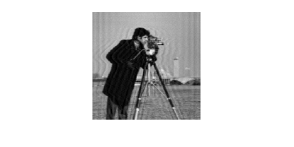
(d)	(e)	(f)

Figure 1. Example 4.4 (bandw=$7$ and NoiseLevel$=0.01$): Original (a) and blurred–noisy (b) images; Restored images by TSTMR (c), IRcgls (d), IRhybrid_lsqr^∗ (e) and IRhybrid_lsqr^∗∗(f).

We end this subsection by a test problem from [11] for which the matrix $A$ in (18) is non-square.

Example 4.5.

We consider the 2D fan-beam linear-detector tomography test problem from IR Tools toolbox. More precisely, we use the function $[A,\tilde{g},f]$ = fanlineartomo$(n,\theta,p)$ inside the toolbox which exploits the “line model” to create a 2D X-ray tomography test problem with an $n\times n$ pixel domain. The vector $\theta$ in the function includes projection angles (in degrees) and the parameter $p$ is associated with the number of rays for each angle. Here we worked with default values of $\theta$ and $p$, i.e., $\theta=0:2:358$ and $p={\rm round(sqrt}(2)*n)$, resulting in a coefficient matrix $A$ of size $\ell\times n^{2}$ where $\ell={\rm length(\theta)}*p$. We report the numerical results for Example 4.5 in Tables 11 and 12 for four different values of $n$. Now IRhybrid_lsqr^∗∗ is more feasible compared to Example 4.4. While the proposed method is no longer always the fastest in terms of CPU-time (especially for larger problems), its performance appears to be quite robust and the method results in smaller errors and higher PSNRs than can be obtained with the other methods. In the largest case, $A$ is approximately of size $25,000\times 10,000$ and contains just over $2,000,000$ nonzero entries.

Table 11. Example 4.5: Comparison results for 2D fan-beam linear-detector tomography test problem (NoiseLevel$=0.01$ and and max${}_{\rm itcg}=20$)

$n$	Determination of	Method			Err	CPU	Iter	PSNR
	regularization parameter
25	N/A	TSTMR			0.0320	0.01	2	42.3
	N/A	IRcgls			0.0508	0.09	21	38.3
	DP	IRhybrid_lsqr∗			0.0490	0.10	23	38.6
	WGCV	IRhybrid_lsqr∗∗			0.0532	0.11	26	37.9
50	N/A	TSTMR			0.0451	0.04	2	39.0
	N/A	IRcgls			0.0788	0.11	22	34.2
	DP	IRhybrid_lsqr∗			0.0759	0.12	24	34.6
	WGCV	IRhybrid_lsqr∗∗			0.0718	0.14	29	35.0
75	N/A	TSTMR			0.0705	0.16	3	35.2
	N/A	IRcgls			0.1169	0.13	21	30.8
	DP	IRhybrid_lsqr∗			0.1148	0.14	23	30.9
	WGCV	IRhybrid_lsqr∗∗			0.1062	0.19	30	31.6
100	N/A	TSTMR			0.1268	0.29	3	30.3
	N/A	IRcgls			0.1749	0.17	21	27.5
	DP	IRhybrid_lsqr∗			0.1706	0.19	23	27.7
	WGCV	IRhybrid_lsqr∗∗			0.1560	0.28	33	28.5

Table 12. Example 4.5: Comparison results for 2D fan-beam linear-detector tomography test problem (NoiseLevel$=0.03$ and max${}_{\rm itcg}=20$)

$n$	Determination of	Method			Err	CPU	Iter	PSNR
	regularization parameter
25	N/A	TSTMR			0.0599	0.01	2	36.9
	N/A	IRcgls			0.1078	0.09	15	31.8
	DP	IRhybrid_lsqr∗			0.1155	0.08	15	31.2
	WGCV	IRhybrid_lsqr∗∗			0.1555	0.09	15	28.6
50	N/A	TSTMR			0.1066	0.04	2	31.6
	N/A	IRcgls			0.1705	0.10	14	27.5
	DP	IRhybrid_lsqr∗			0.1609	0.10	15	28.0
	WGCV	IRhybrid_lsqr∗∗			0.1901	0.12	17	26.6
75	N/A	TSTMR			0.1675	0.10	2	27.7
	N/A	IRcgls			0.2231	0.11	12	25.2
	DP	IRhybrid_lsqr∗			0.2254	0.12	12	25.1
	WGCV	IRhybrid_lsqr∗∗			0.2122	0.15	15	25.6
100	N/A	TSTMR			0.2406	0.21	2	24.7
	N/A	IRcgls			0.2550	0.12	11	24.2
	DP	IRhybrid_lsqr∗			0.2502	0.14	12	24.3
	WGCV	IRhybrid_lsqr∗∗			0.2396	0.19	16	24.7

5. Conclusions

In this paper we have introduced a new class of two-step iterative methods for solving linear systems of equations. To construct these type of methods, the approximate solution at each sub-step of a standard two-step iterative method is computed by minimizing its residual norm over a certain two-dimensional subspace. The resulting approach is called the TSTMR method and, under certain conditions, can be proved to either converge in the limit or to break down after determining the exact solution in a finite number of steps. Furthermore, we showed how the method can be adapted to solve a class of augmented systems corresponding to (shifted) normal equations associated with least-squares problems arising from the discretization of ill-posed problems. An advantage of this method over established Krylov subspace solvers like GMRES is the low amount of memory required for its implementation.

For well-posed problems, first, we demonstrated experimentally that the TSTMR method outperforms the MRHSS method for test problems of the convection-diffusion type examined in [20]. We further used the proposed method for solving a block linear system of equations corresponding to a 3D coupled Stokes-Darcy flow problem. We observed that the proposed method provides more accurate solutions in comparison with the best approach in the recent paper [5] while both methods exhibit similar performance in terms of the required CPU times to satisfy a given stopping criterion.

For discrete ill-posed problems arising in image deblurring and tomography, the competitiveness of the TSTMR method with several other popular iterative schemes was also demonstrated by numerical experiments.

Future work should focus on analyzing the convergence properties of the proposed methods when implemented inexactly. While we found experimentally that the convergence of the method is not much affected by inexact inner solves, a better theoretical understanding of the convergence of inexact variants of TSTMR would be desirable.

Acknowledgement. The authors would like to thank Scott Ladenheim for providing the test problem in Example 4.2. The work of M. Benzi was supported in part by “Fondi per la Ricerca di Base” of the Scuola Normale Superiore di Pisa.

References

• [1] A. Ameri and F. P. A. Beik, Note to the convergence of minimum residual HSS method, Journal of Mathematical Modeling, 9 (2021) 323–330.
• [2] Z.-Z. Bai, G. H. Golub and M. K. Ng, Hermitian and skew–Hermitian splitting methods for non-Hermitian positive definite linear systems, SIAM Journal on Matrix Analysis and Applications, 24 (2003) 603–626.
• [3] M. Benzi and G. H. Golub, A preconditioner for generalized saddle point problems, SIAM Journal on Matrix Analysis and Applications, 26 (2004) 20–41.
• [4] M. Benzi and M. K. Ng, Preconditioned iterative methods for weighted Toeplitz least squares problems, SIAM Journal on Matrix Analysis and Applications, 27 (2006) 1106–1124.
• [5] F. P. A. Beik and M. Benzi, Preconditioning techniques for the coupled Stokes–Darcy problem: spectral and field-of-values analysis, Numerische Mathematik, 150 (2022) 257–298.
• [6] M. Cai, M. Mu and J. Xu, Preconditioning techniques for a mixed Stokes/Darcy model in porous media applications, Journal of Computational and Applied Mathematics, 233 (2009) 346–355.
• [7] P. Chidyagwai, S. Ladenheim and D. B. Szyld, Constraint preconditioning for the coupled Stokes-Darcy system, SIAM Journal on Scientific Computing, 38 (2016) A668–A690.
• [8] J. Chung, J. G. Nagy and D. P. O’Leary, A weighted–GCV method for Lanczos-hybrid regularization, Electronic Transactions on Numerical Analysis, 28 (2008) 149–167.
• [9] J. Cui, G. Peng, Q. Lu and Z. Huang, Modified special HSS method for discrete ill-posed problems and image restoration, International Journal of Computer Mathematics, 97 (2020) 739–758.
• [10] H. C. Elman, D. J. Silvester and A. J. Wathen, Finite Elements and Fast Iterative Solvers: with applications in incompressible fluid dynamics, Oxford University Press, USA, 2005.
• [11] S. Gazzola, P. C. Hansen and J. G. Nagy, IR Tools: a MATLAB package of iterative regularization methods and large-scale test problems, Numerical Algorithms, 81 (2019) 773–811.
• [12] G. H. Golub, M. Heath and G. Wahba, Generalized cross–validation as a method for choosing a good ridge parameter, Technometrics, 21 (1979) 215–223.
• [13] G. H. Golub and D. Vanderstraeten, On the preconditioning of matrices with skew-symmetric splittings, Numerical Algorithms, 25 (2000) 223–239.
• [14] P. C. Hansen, Discrete Inverse Problems: Insight and Algorithms, SIAM, Philadelphia, 2010.
• [15] P. C. Hansen, Rank–deficient and Discrete Ill-posed Problems: Numerical Aspects of Linear Inversion, SIAM, Philadelphia, 1998.
• [16] P. C. Hansen, Regularization tools: A MATLAB package for analysis and solution of discrete ill-posed problems, Numerical Algorithms, 6 (1994) 1–35.
• [17] D. Loghin and A. J. Wathen, Analysis of preconditioners for saddle–point problems, SIAM Journal on Scientific Computing, 25 (2004) 2029–2049.
• [18] X.-G. Lv, T.-Z. Huang, Z.-B. Xu, X.-L. Zhao, A special Hermitian and skew-Hermitian splitting method for image restoration, Applied Mathematical Modelling, 37 (2013) 1069–1082.
• [19] Y. Saad, Iterative Methods for Sparse Linear Systems, second ed., SIAM, Philadelphia, 2003.
• [20] A. L. Yang, Y. Cao and Y. J. Wu, Minimum residual Hermitian and skew-Hermitian splitting iteration method for non-Hermitian positive definite linear systems, BIT Numerical Mathematics, 59 (2019) 299–319.
• [21] A. L. Yang, On the convergence of the minimum residual HSS iteration method, Applied Mathematics Letters, 94 (2019) 210–216.