A mixed-dimensional model for direct current simulations in presence of a thin high-resistivity liner

Abstract

In this work we present a mixed-dimensional mathematical model to obtain the electric potential and current density in direct current simulations when a thin liner is included in the modelled domain. The liner is used in landfill management to prevent leakage of leachate from the waste body into the underground and is made of a highly-impermeable high-resistivity plastic material. The electrodes and the liner have diameters and thickness respectively that are much smaller than their other dimensions, thus their numerical simulation might be too costly in an equi-dimensional setting. Our approach is to approximate them as objects of lower dimension and derive the corresponding equations. The obtained mixed-dimensional model is validated against laboratory experiments of increasing complexity showing the reliability of the proposed mathematical model.

1 Introduction

The direct current (DC) resistivity method is a geophysical technique used for non-invasive investigations in a wide range of applications and is best suited to detect subsurface saturation and pollution, as underground fluids and dissolved ions strongly control subsurface resistivities [BK05].

Our target application is the geoelectrical monitoring of municipal solid waste landfills (MSWLFs). In more detail, we want to explore the capability of the DC method to characterize the high- or low-density polyethylene (HDPE or LDPE) liner that is generally placed underneath the landfill to prevent leachate leakage in the underground. The method is promising to discriminate between the plastic liner, that is practically an electrical insulator, from leachate that can have resistivity as low as 1 [$\mathrm{\SIUnitSymbolOhm}\text{\,}\mathrm{m}$]. The scientific literature reports several case studies where geoelectrical methods have been applied to landfills with different design, size, and confining materials, consisting of diverse types of waste, and located either in urbanized or remote areas [BDOH00, Mej00, LDR10, VSP⁺11, DPC⁺13, TVFT14, DFL⁺18]. In many cases, the aim of the studies was to delineate the extent of the buried waste body and DC measurements have been conducted together with Induced Polarization ones ([DRL10, DC17]). Some numerical and down-scaled laboratory studies have been devoted to detecting and locating ruptures and holes in the plastic liner with set ups with different levels of complexity ([Fra97, BDR97, BD03, LRQ⁺19, AHZA20]). However, the geoelectrical method aimed to analyse the integrity of the geomembrane at the field scale still lacks thorough validation and issues related to the survey design, the investigation depth and to the spatial resolution need to be addressed ([AFS⁺21]).

In the simplest DC configuration, two electrodes inject current $I$ in the investigated medium and two electrodes measure the potential difference $\Delta V$. The ratio $\Delta V/I$ multiplied by a factor $K$ related to the geometrical arrangement of the electrodes yields the apparent electrical resistivity $\rho_{a}$, which is a function of the resistivities of the investigated media and changes according to $K$.

Up to date, geoelectrical equipment easily handles tens to hundreds of electrodes for 2D, 3D and 4D (i.e., 3D-time lapse) surveys ([LRDC19]) allowing for the tomographic reconstruction of the subsurface resistivities (electrical resistivity tomography - ERT). ERT constitutes a non-linear and ill-posed inverse problem in which the non-linearity is due to the equation linking the subsurface resistivity values to the measured apparent resistivity data, whereas the ill-posedness is mainly related to incomplete data coverage, considerable number of unknown parameters to be estimated and noise contamination in the data ([Men18]). Whether the inversion of geoelectrical data is performed with a deterministic or probabilistic approach, a robust and effective numerical code is needed to solve the forward problem. Though both commercial (e.g., [Lok22]) and open-source forward geoelectrical codes ([RGW17, BSB⁺20]) have been developed, in this work we propose a mathematical model taking into account the peculiar aspects of the geoelectrical monitoring of MSWLFs related to the different sizes of the elements to be considered. The liner is a few millimetres thick and has lateral extent of tens of thousands square meters; similarly, the ratio of the diameter to the length of the electrodes is typically one to forty centimetres ( [RG11]). It is clear that representing these items as three-dimensional objects requires a computational grid that might be unnecessary refined, as discussed in [BBF⁺20] for a similar context, with obvious computational cost. Accordingly, we introduce new conceptual models to lighten the computational cost of the forward problem while maintaining the accuracy. We consider a model reduction technique to approximate the electrodes as one-dimensional objects of the same length as their three-dimensional representation, and the liner as two-dimensional object of the same extent. Example of model reduction to one-dimensional objects can be found, for instance, in [Pea78, Pea83] and more recently in [CLZ19, GKNW19, GKN20, KLMZ21, BGS22] while for two-dimensional objects in [MJR05, DS12, FK18, FKS19, NBFK19]. A new set of equations will be derived for the electrodes and the liner along with appropriate interface conditions for their coupling with the surrounding domain. With the reduced model, a coarser grid can be used, or bigger problems can be solved, which will reduce ill-posedness and computational cost.

The outcomes of the model-based code are then compared with results obtained through down-scaled experiments in the laboratory and, whenever possible, with theoretical results. In particular, we consider several settings by changing the depth of the geomembrane and the presence or absence of holes.

To solve the model numerically two cell-centred finite volume schemes, multi-point flux approximation (MPFA) [Aav07b, Aav02] and two-point flux approximation (TPFA) [Aav07a] methods, are exploited and the results are compared with experimental data to identify the most suitable approach in terms of computational costs and accuracy.

This article is organized as follows. In Section 2, first we introduce the mathematical model for a three-dimensional domain, and then the mixed-dimensional model for the electrodes and the liner. Section 3 is devoted to the spatial discretization of the equations by discussing appropriate strategies to make their solution more efficient. In Section 4 we consider two different settings to validate the proposed model: in the first one the liner is flat and changes its depth, while in the second one the liner has a box shape with the possible presence of a hole. Finally, we draw the conclusions in Section 5.

2 The mathematical model

We indicate the domain where the geoelectrical equations will be applied with $\Upsilon\subset\mathbb{R}^{3}$, with boundary $\partial\Upsilon$ and outward unit normal $\bm{n}_{\partial}$. We consider the following main variables: $\bm{E}:\Upsilon\rightarrow\mathbb{R}^{3}$, the electric field in [$\mathrm{V}\text{\,}{\mathrm{m}}^{-1}$], $\bm{J}:\Upsilon\rightarrow\mathbb{R}^{3}$, the current density field in [$\mathrm{A}\text{\,}{\mathrm{m}}^{-2}$], and $\varphi:\Upsilon\rightarrow\mathbb{R}$, the electric potential in [$\mathrm{V}$].

We present now the governing equations. Ohm-Kirchhoff’s law states that $\bm{J}=\sigma\bm{E}$, with $\sigma:\Upsilon\rightarrow\mathbb{R}_{>0}$ the electric conductivity of the medium in [$\mathrm{S}\text{\,}{\mathrm{m}}^{-1}$]. The latter is the inverse of the electric resistivity $\rho$, measured in [$\mathrm{\SIUnitSymbolOhm}\text{\,}\mathrm{m}$]. Moreover, as a consequence of the static Maxwell-Faraday equation, $\nabla\times\bm{E}=\bm{0}$, and by the Helmholtz decomposition we get that the electric field $\bm{E}$ can be related to the gradient of the electric potential $\varphi$ as $\bm{E}=-\nabla\varphi$. We can thus establish a constitutive relation between the current density field $\bm{J}$ and the electric potential $\varphi$ as follow

$$\bm{J}+\sigma\nabla\varphi=\bm{0}.$$ (1)

Gauss’ law, or charge conservation equation for $\bm{J}$, can be expressed as

$$\nabla\cdot\bm{J}=q,$$ (2)

with $q:\Upsilon\rightarrow\mathbb{R}$ being the source of volumetric charge density in [$\mathrm{A}\text{\,}{\mathrm{m}}^{-3}$]. For simplicity, we consider an isolated body so at the boundary $\partial\Upsilon$ we set $\bm{J}\cdot\bm{n}_{\partial}=0$. By combining (1) and (2) the problem can be written as:

Problem 1 (The DC problem).

The direct current problem is: find $(\bm{J},\varphi)$ in $\Upsilon$ such that

$$\begin{aligned} &\begin{aligned} &\bm{J}+\sigma\nabla\varphi=\bm{0}\\ &\nabla\cdot\bm{J}=q\end{aligned}&&\text{in }\Upsilon\\ &\bm{J}\cdot\bm{n}_{\partial}=0&&\text{on }\partial\Upsilon\end{aligned}$$

In Subsection 2.1, we present a suitable model for the electrodes represented as objects of dimension 1 immersed in $\Upsilon$ and in Subsection 2.2 the bi-dimensional model for the liner.

2.1 A model for the electrodes

Depending on the chosen electrode configuration, multiple electrodes are immersed in $\Upsilon$ and can be used, in pairs, to inject electrical current and measure the electric potential differences.

We want to introduce an effective and efficient mathematical model able to describe their influence in Problem 1. For simplicity, we consider a single electrode, being immediate the extension to multiple (separated) electrodes, and set $q=0$. Even if an electrode is a three-dimensional object, typically a cylinder of stainless steel, its radius is very small compared to its length and domain size. Typically, the ratio between its radius and length is in the order of 1/30 $\sim$ 1/50. Our idea is thus to approximate the electrode by an object of dimension 1, making the gridding process much easier and with fewer cells, essential when dealing with real geometries.

Let us consider Figure 1 on the left where a three-dimensional electrode $\Gamma$ is immersed in $\Upsilon$, with $\mathring{\Gamma}\cap\mathring{\Upsilon}=\emptyset$. We assume that one end of the electrode is in contact with the top of $\partial\Upsilon$.

Figure 1: An electrode $\Gamma$ represented as three-dimensional object (right) and the reduced electrode $\gamma$ as one-dimensional object (left).

We suppose $\Gamma$ to be a cylinder with radius $r$ and longitudinal axis $\gamma$ of length $l$, described as

$$\Gamma=D\times\gamma\quad\text{with}\quad D=\{(\xi\cos\theta,\xi\sin\theta)\text{ with }\xi\in[0,r)\text{ and }\theta\in[0,2\pi)\}.$$

We indicate with $\bm{v}_{\Gamma}$ the unit vector aligned with line $\gamma$. The equations of Problem 1 apply to $\Gamma$ with coefficients that are different than those of the surrounding domain $\Upsilon$. We indicate variables in $\Gamma$ with a subscript. To couple the two systems, suitable conditions are needed on the common boundary between $\Upsilon$ and $\Gamma$, we call $\partial_{i}\Gamma=\overline{\Gamma}\cap\overline{\Upsilon}$ the internal part of $\partial\Gamma$. Since the electrode is a cylinder, we further divide $\partial_{i}\Gamma$ into two disjoint portions $\partial_{l}\Gamma$ and $\partial_{b}\Gamma$, the former being the lateral surface and the latter the bottom one. Finally, $\partial_{t}\Gamma$ is the top part of the boundary of $\Gamma$, which is not in contact with the interior of $\Upsilon$. Conservation of the current density through $\partial_{i}\Gamma$ and continuity of the electric potential are required,

$$\begin{aligned} &\bm{J}\cdot\bm{n}_{\Gamma}=\bm{J}_{\Gamma}\cdot\bm{n}_{\Gamma}\\ &\varphi=\varphi_{\Gamma}\end{aligned}\quad\text{on }\partial_{i}\Gamma$$

where $\bm{n}_{\Gamma}$ is the unit normal of $\partial_{i}\Gamma$ pointing from $\Upsilon$ toward $\Gamma$.

To avoid excessive refinement of the computational grid to capture the three-dimensional nature of the electrode, we employ a model reduction strategy by approximating $\Gamma$ with its centre line $\gamma$ while the surrounding domain, with an abuse of notation, will be still indicated with $\Upsilon$, see Figure 1 on the right. We will derive a new set of equations for $\gamma$ and coupling conditions between $\gamma$ and $\Upsilon$, by following the approach presented in [Pea78, Pea83, DQ08, GKNW19, GKN20, KLMZ21] derived for wells in porous media and here adapted to the electrodes. We assume the following:

Assumption 1 (Electrode radius).

We assume that the radius $r$ of the electrode is much smaller than any other characteristic length in the domain.

Assumption 2 (Lateral exchange).

We assume that the current density is exchanged between the electrode and the surrounding media through the lateral boundary of the electrode $\partial_{l}\Gamma$, the exchange through $\partial_{b}\Gamma$ is assumed to be negligible.

The line current density exchanged between the electrode, now represented as $\gamma$, and the surrounding media is denoted as $j_{\gamma}$ in [$\mathrm{A}\text{\,}{\mathrm{m}}^{-1}$] and approximated by the relation

$$j_{\gamma}+\sigma_{\gamma}(\varphi_{\gamma}-\varphi)=0\quad\text{on }\gamma,$$ (3)

where $\sigma_{\gamma}$ in [$\mathrm{S}\text{\,}{\mathrm{m}}^{-1}$] is the conductivity of the interface between the electrode and the surrounding media, whose meaning will be discussed in the following. The reduced variables for the electrode $\varphi_{\gamma}$ in [$\mathrm{V}$] and $\bm{J}_{\gamma}$ now in [$\mathrm{A}$] are defined as

$$\varphi_{\gamma}(z)=\frac{1}{\pi r^{2}}\int_{D}\varphi_{\Gamma}(\xi,\theta,z)d\xi d\theta\quad\text{and}\quad\bm{J}_{\gamma}(z)=\int_{D}(\bm{v}_{\Gamma}\otimes\bm{v}_{\Gamma})\bm{J}_{\Gamma}(\xi,\theta,z)d\xi d\theta.$$

By following the model reduction procedure considered in the aforementioned works, we can introduce a new model for the electrode represented as an object $\gamma$ of dimension $n-2$

$$\begin{aligned} &\bm{J}_{\gamma}+\pi r^{2}\sigma_{\Gamma}\nabla\varphi_{\gamma}=\bm{0}\\ &\nabla\cdot\bm{J}_{\gamma}-j_{\gamma}=0\end{aligned}\quad\text{in }\gamma,$$ (4)

where the gradient and divergence are now computed along $\gamma$. The second equation is a conservation equation which accounts for the current along $\gamma$ and its exchange with $\Upsilon$, represented as $j_{\gamma}$. On the base of assumption 2, we set the so-called tip condition on the bottom boundary of $\gamma$

$$\bm{J}_{\gamma}\cdot\bm{v}_{\Gamma}=0\quad\text{on }\partial_{b}\gamma.$$ (5)

As mentioned, the electrodes inject a prescribed current density $\overline{J}_{\Gamma}$ in [$\mathrm{A}\text{\,}{\mathrm{m}}^{-2}$], or measure potential difference, thus $\overline{J}_{\Gamma}=0$ in this latter case. Accordingly, we employ one of the following conditions on $\partial_{t}\gamma$:

$$\begin{aligned} &\bm{J}_{\gamma}\cdot\bm{n}_{\partial}=i_{\gamma}\\ &\bm{J}_{\gamma}\cdot\bm{n}_{\partial}=0\end{aligned}\quad\text{on }\partial_{t}\gamma,$$

for current and potential electrodes, respectively, with $i_{\gamma}=\pi r^{2}\overline{J}_{\Gamma}$ being the current in [$\mathrm{A}$].

In $\Upsilon$, the electrode is seen as an immersed line acting as source/sink of electric current. Introducing the Dirac delta $\delta_{\gamma}$ distributed along $\gamma$ with measure [${\mathrm{m}}^{-2}$], the new set of equations for $\Upsilon$ reads

$$\begin{aligned} &\bm{J}+\sigma\nabla\varphi=\bm{0}\\ &\nabla\cdot\bm{J}+j_{\gamma}\delta_{\gamma}=0\end{aligned}\quad\text{in }\Upsilon$$ (6)

Solutions of the previous equations exhibit a logarithmic singularity in $\varphi$ with strong derivatives in the vicinity of $\gamma$. Assuming a radial current density exiting from the electrode, following the approach given [Pea78, Pea83], it is possible to write the coefficient in (3) as

$$\sigma_{\gamma}=\frac{2\pi\sigma}{\ln(r_{e}/r)+S},$$

which is a semi-discrete parameter that is used to mimic the effect of the singularity around $\gamma$, when a discretization in space is applied, without the need of over-refining the grid. The parameter $r_{e}$ in [$\mathrm{m}$] is the radius at which the electric potential in the medium $\varphi$ is equal to the averaged grid cell potential. $r_{e}$ is normally taken equal to $r_{e}\approx 0.2h$ with $h$, in [$\mathrm{m}$], the cell diameter. $S$ in [$\cdot$] is the so-called skin-factor, which gives an additional electric potential drop due to the actual features of the electrode and of the surrounding zone. $S$ can be used to model rust or other imperfections of the electrode, and also to model the imperfect contact between the electrode and the ground. We are finally ready to introduce the new mixed-dimensional problem.

Problem 2 (The mixed-dimensional electrode DC problem).

Find $(\bm{J},\varphi)$ in $\Upsilon$ and $(j_{\gamma},\bm{J}_{\gamma},\varphi_{\gamma})$ in $\gamma$ such that

$$\begin{aligned} &\bm{J}+\sigma\nabla\varphi=\bm{0}\\ &\nabla\cdot\bm{J}+j_{\gamma}\delta_{\gamma}=0\end{aligned}\quad\text{in }\Upsilon,\qquad\begin{aligned} &\bm{J}_{\gamma}+\pi r^{2}\sigma_{\Gamma}\nabla\varphi_{\gamma}=\bm{0}\\ &\nabla\cdot\bm{J}_{\gamma}-j_{\gamma}=0\end{aligned}\quad\text{in }\gamma,$$

coupled with the following interface condition

$$j_{\gamma}+\sigma_{\gamma}(\varphi_{\gamma}-\varphi)=0,\quad\text{on }\gamma$$

and with boundary conditions given by

$$\begin{aligned} &\bm{J}\cdot\bm{n}_{\partial}=0&&\text{on }\partial\Upsilon,\\ &\bm{J}_{\gamma}\cdot\bm{n}_{\partial}=\pi r^{2}\overline{J}_{\Gamma}&&\text{on }\partial_{t}\gamma,\\ &\bm{J}_{\gamma}\cdot\bm{v}_{\Gamma}=0&&\text{on }\partial_{b}\gamma.\end{aligned}$$

2.2 A model for the liner

A liner is placed below the waste body to avoid the infiltration of leachate in the underground, that can be dangerous for the groundwater. For simplicity, we assume that the liner consists of a planar portion of a highly resistive geomembrane whose thickness is much smaller than other lengths in the domain. For real applications, the ratio between its thickness and lateral extension is in the order of $\sim 10^{-5}$. To simplify gridding and avoid excessive refinement in representing the liner as a three-dimensional object we present a two-dimensional model of the liner with suitable coupling conditions with the surrounding media.

In the case of a liner composed by several planar parts, e.g. having a box shape, we will apply the new model to each part and use suitable conditions to connect them. This aspect will be detailed later.

Let us consider Figure 2 on the left where a liner $\Lambda$ is immersed in $\Upsilon$.

Figure 2: The liner $\Lambda$ represented as three-dimensional object (right) and the reduced liner $\lambda$ as two dimensional object (left).

It can be described as a domain with thickness $\varepsilon$ in $[$\mathrm{m}$]$ and central (portion of a) plane $\lambda$,

$$\Lambda=\lambda\times\left(-\frac{\varepsilon}{2},\frac{\varepsilon}{2}\right).$$

We indicate with $\bm{n}_{\Lambda}$ the unit normal to the top boundary of $\Lambda$ pointing from $\Upsilon$ toward $\Lambda$. Equations of Problem 1 apply also to $\Lambda$ with different conductivity than the surrounding $\Upsilon$, therefore, as done for the electrode, we propose now a suitable reduced model where the liner is approximated with its central plane $\lambda$, by following the same approach as in [MJR05, DS12, NBFK19, FS20]. First, we divide the boundary $\partial\Lambda$ of $\Lambda$ into two parts: the lateral surface of thickness $\varepsilon$ is named $\partial_{l}\Lambda$, and the bottom and top surfaces are identified as $\partial_{s}\Lambda$. If the liner ends inside $\Upsilon$, we can identify the portion of its lateral boundary that is in contact with the internal part of $\Upsilon$. We call this internal part of the boundary as $\partial_{i}\Lambda\subset\partial_{l}\Lambda$. Let us state the following assumptions.

Assumption 3 (Liner thickness).

We assume that the thickness $\varepsilon$ of the liner is much smaller than any other sizes in the domain.

Assumption 4 (Lateral exchange).

We assume that current density is exchanged between the liner and the surrounding media through $\partial_{s}\Lambda$, the exchange though $\partial_{i}\Lambda$ is assumed to be negligible.

We substitute the equi-dimensional representation of the liner $\Lambda$ with its lower-dimensional counterpart $\lambda$, so that the mesh size is not constraned by its thickness $\varepsilon$. We present now the mathematical model for $\lambda$. Note that the liner is in contact with $\Upsilon$ with its top and bottom surfaces.

For each side of $\lambda$, the current density exchanged between the liner and the surrounding media, following (3), is denoted as $j_{\lambda}$ in [$\mathrm{A}\text{\,}{\mathrm{m}}^{-2}$] and approximated by

$$\varepsilon j_{\lambda}+\sigma_{\lambda}(\varphi_{\lambda}-\varphi)=0\quad\text{on }\lambda.$$ (7)

Being $\lambda$ of codimension 1, it does not introduce singular solutions and thus we do not have the need to tune $\sigma_{\lambda}$ as we did for $\sigma_{\gamma}$. Indeed, the value of $\sigma_{\lambda}$ in [$\mathrm{S}\text{\,}{\mathrm{m}}^{-1}$] simply represents the conductivity of the liner along its normal. The reduced variables are $\varphi_{\lambda}$ in [$\mathrm{V}$] and $\bm{J}_{\lambda}$ now in [$\mathrm{A}\text{\,}{\mathrm{m}}^{-1}$] and defined as

$$\varphi_{\lambda}(x,y)=\frac{1}{\varepsilon}\int_{-\frac{\varepsilon}{2}}^{\frac{\varepsilon}{2}}\varphi_{\Lambda}(x,y,z)dz\quad\text{and}\quad\bm{J}_{\gamma}(x,y)=\int_{-\frac{\varepsilon}{2}}^{\frac{\varepsilon}{2}}(I-\bm{n}_{\Lambda}\otimes\bm{n}_{\Lambda})\bm{J}_{\Lambda}(x,y,z)dz,$$

with $I$ the identity matrix. We can now introduce a model for the liner represented as an object $\lambda$ of dimension $n-1$

$$\begin{aligned} &\bm{J}_{\lambda}+\varepsilon\sigma_{\Lambda}\nabla\varphi_{\lambda}=\bm{0}\\ &\nabla\cdot\bm{J}_{\lambda}-j_{\lambda}=0\end{aligned}\quad\text{in }\lambda.$$

The gradient and divergence are now computed over the plane $\lambda$. To couple this model with Problem 1 in $\Upsilon$, we simply require current conservation so that $\bm{J}\cdot\bm{n}_{\Lambda}=j_{\lambda}$ on each side of $\lambda$. In the experiments we will consider the boundary of $\lambda$ to be in contact with $\partial\Upsilon$, and thus inheriting the same boundary conditions, or immersed into $\Upsilon$ in which case we impose null current exhange, as in (5).

When the liner geometry is more complex but can still be split into multiple planar polygons, we can follow the same strategy for each one of them. Since the liner is composed by a homogeneous material, at the interface between two planes we simply require that the current density is conserved and that the electric potential is continuous.

The problem is thus formalized as follows.

Problem 3 (The mixed-dimensional liner DC problem).

Find $(\bm{J},\varphi)$ in $\Upsilon$ and $(j_{\lambda},\bm{J}_{\lambda},\varphi_{\lambda})$ in $\lambda$ such that

$$\begin{aligned} &\bm{J}+\sigma\nabla\varphi=\bm{0}\\ &\nabla\cdot\bm{J}=0\end{aligned}\quad\text{in }\Upsilon\qquad\begin{aligned} &\bm{J}_{\lambda}+\varepsilon\sigma_{\Lambda}\nabla\varphi_{\lambda}=\bm{0}\\ &\nabla\cdot\bm{J}_{\lambda}-j_{\lambda}=0\end{aligned}\quad\text{in }\lambda$$

coupled with the following interface condition on both sides of $\lambda$

$$\varepsilon j_{\lambda}+\sigma_{\lambda}(\varphi_{\lambda}-\varphi)=0\quad\text{on }\lambda$$

with boundary conditions given by

$$\begin{aligned} &\bm{J}\cdot\bm{n}_{\partial}=0&&\text{on }\partial\Upsilon\\ &\bm{J}_{\lambda}\cdot\bm{n}_{\partial}=0&&\text{on }\partial\lambda\end{aligned}$$

2.3 The complete mixed-dimensional model

For simplicity we assume that the electrodes and the liner are not intersecting nor in contact, so the global problem considers both contributions presented in Problem 2 and Problem 3 in a straightforward case. The mixed-dimensional model consider a set of $N$ electrodes, indexed with $i=1,\ldots,N$, and a single liner, see Figure 3.

Figure 3: Schematic representation of the mixed-dimensional objects: the three-dimensional domain $\Upsilon$, the two-dimensional liner $\lambda$, and the one-dimensional electrodes $\gamma_{i}$.

The equations are presented as following.

Problem 4 (The mixed-dimensional DC problem).

Find $(\bm{J},\varphi)$ in $\Upsilon$, $(j_{\gamma_{i}},\bm{J}_{\gamma_{i}},\varphi_{\gamma_{i}})$ in $\gamma_{i}$ for $i=1,\ldots,N$ and $(j_{\lambda},\bm{J}_{\lambda},\varphi_{\lambda})$ in $\lambda$ such that

$$\begin{aligned} &\bm{J}+\sigma\nabla\varphi=\bm{0}\\ &\nabla\cdot\bm{J}+{\textstyle\sum_{i}}j_{\gamma_{i}}\delta_{\gamma_{i}}=0\end{aligned}\quad\text{in }\Upsilon\qquad\begin{aligned} &\bm{J}_{\gamma_{i}}+\pi r_{i}^{2}\sigma_{\Gamma_{i}}\nabla\varphi_{\gamma_{i}}=\bm{0}\\ &\nabla\cdot\bm{J}_{\gamma_{i}}-j_{\gamma_{i}}=0\end{aligned}\quad\text{in }\gamma_{i}\qquad\begin{aligned} &\bm{J}_{\lambda}+\varepsilon\sigma_{\Lambda}\nabla\varphi_{\lambda}=\bm{0}\\ &\nabla\cdot\bm{J}_{\lambda}-j_{\lambda}=0\end{aligned}\quad\text{in }\lambda$$

coupled with the following interface condition

$$j_{\gamma_{i}}+\sigma_{\gamma_{i}}(\varphi_{\gamma_{i}}-\varphi)=0\quad\text{on }\gamma_{i}\qquad\varepsilon j_{\lambda}+\sigma_{\lambda}(\varphi_{\lambda}-\varphi)=0\quad\text{on }\lambda$$

with boundary conditions given by

$$\begin{aligned} &\bm{J}\cdot\bm{n}_{\partial}=0&&\text{on }\partial\Upsilon\\ &\bm{J}_{\lambda}\cdot\bm{n}_{\partial}=0&&\text{on }\partial\lambda\end{aligned}\qquad\begin{aligned} &\bm{J}_{\gamma_{i}}\cdot\bm{n}_{\partial}=\pi r_{i}^{2}\overline{J}_{\Gamma_{i}}&&\text{on }\partial_{t}\gamma_{i}\\ &\bm{J}_{\gamma_{i}}\cdot\bm{v}_{\Gamma_{i}}=0&&\text{on }\partial_{b}\gamma_{i}\\ \end{aligned}$$

By balancing the current density imposed on the boundary, Problem 4 admits a unique solution for $(\bm{J},\bm{J}_{\gamma_{i}},j_{\gamma_{i}},\bm{J}_{\lambda},j_{\lambda})$, however the electric potentials $(\varphi,\varphi_{\gamma_{i}},\varphi_{\lambda})$ are defined up to a constant $c\in\mathbb{R}$. To uniquely define this constant it is possible to consider different strategies like imposing the following null average condition

$$\int_{\Upsilon}\varphi+\sum_{i=1}^{N}\int_{\gamma_{i}}\varphi_{\gamma_{i}}+\int_{\lambda}\varphi_{\lambda}=0.$$

However, in our application, we are interested in potential differences, thus the constant $c$ does not have any practical influence.

3 Numerical approximation

In this section we discuss the numerical approximation of Problem 4, detailing the strategies adopted to represent the mixed-dimensional objects in an efficient and effective way.

We start by considering each object separately and, in Subsection 3.1, we discuss their coupling. By substituting the constitutive equations of Problem 4 into their respective conservation equation, we obtain a problem in primal form in terms only of the electric potentials and $j_{\lambda}$ and $j_{\gamma_{i}}$. Being $\Upsilon$, $\lambda$ and $\gamma_{i}$ objects of dimension 3, 2 and 1, respectively, we construct a simplicial grid composed of tetrahedra for $\Upsilon$, triangles for $\lambda$ and segments for each electrode $\gamma_{i}$. For their construction we rely on Gmsh [GR09]; more details are given in Subsection 3.2.

For the numerical approximation of the problem, we consider two finite-volume cell-centered schemes normally used in the context of flows in porous media and other elliptic problems: the two-point flux approximation (TPFA) as presented in [Aav07a] and the multi-point flux approximation (MPFA) as introduced in [Aav07b, Aav02]. Both schemes have one degree of freedom for each cell but different stencils. TPFA is consistent only for the so called $k$-orthogonal grids, which are grids where the faces normals and the connecting lines between the centers of neighboring cells are orthogonal with respect to the inverse of the diffusion coefficient. Moreover, TPFA is very efficient in the construction and solution of the associated linear problem. MPFA is more expensive but it is convergent for simplicial grids, with only weak regularity requirements on the mesh [Aav07b, Aav02]. We will test in Section 4 the performance of both methods with respect to laboratory experiments.

3.1 Coupling between dimensions

A key aspect in the numerical approximation of Problem 4 is the actual implementation of the coupling conditions between the electrodes, or the liner, and $\Upsilon$. We consider the approach presented in [NBFK19, KBF⁺20], where new grids, called mortar grids, are constructed to handle the coupling between dimensions. In particular, since $j_{\lambda}$ is defined on both sides of the liner and couples it with the surrounding domain, we construct two mortar grids that put in communication $\lambda$ with $\Upsilon$. In principle, these grids may be non-conforming and transfer operators between them need to be constructed that are not, in general, identity maps. To keep our presentation simple, we consider only conforming approximations, see [NBFK19, KBF⁺20] for more details for the non-conforming case.

Since the electrodes are mono-dimensional, and smaller than any other objects present in the problem, to increase the flexibility of the proposed approach, we have considered for them a non-matching discretization meaning that each segment composing $\gamma_{i}$ is immersed in some of the tetrahedra of the $\Upsilon$ grid. A single mortar grid, for each $\gamma_{i}$, is constructed for the coupling. In this case, transfer operators between $\Upsilon$, $\gamma_{i}$ and the mortar grid are accordingly constructed to map variables and then discretize the coupling condition (3). In this case, $j_{\gamma_{i}}$ is the variable defined on the mortar grid that connects $\gamma_{i}$ with $\Upsilon$.

An example of discretized problem is reported in Figure 4, where the liner is approximated with the green grid and the two mortar grids surrounding it are in transparent light green. At the top of the domain, in red, a set of four electrodes is represented as non-matching with the grid of $\Upsilon$.

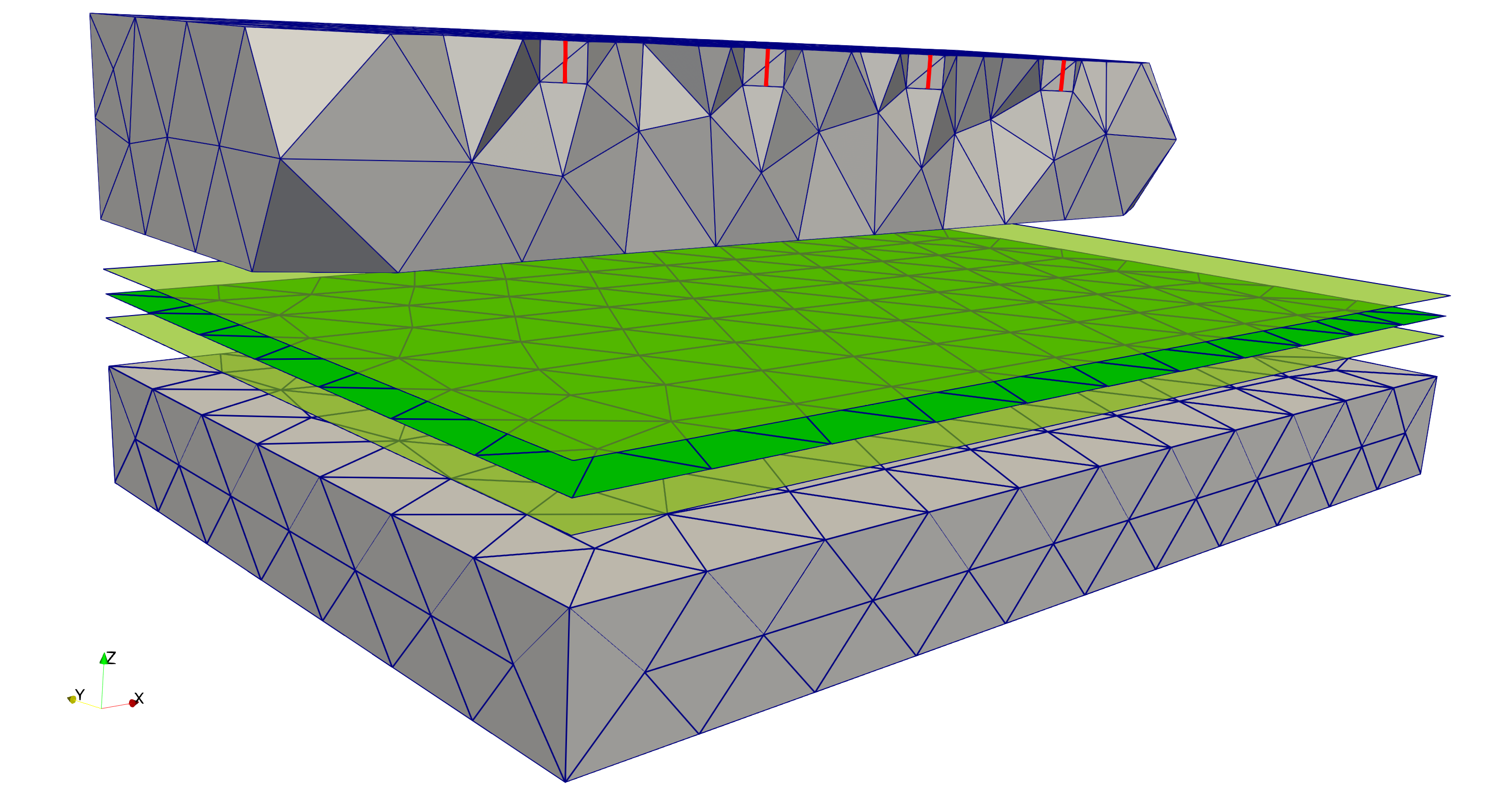
Figure 4: Example of computational grid constructed for the approximation of the problem. The different objects are separated to make the visualization clearer.

3.2 Construction of the computational grid

Another important task in the discretization is to guide the gridding tool to create appropriate grids, [Aav07b, Aav02], and thus limit the numerical error introduced. As discussed before, the grid of the liner is conforming with the surrounding domain, however the electrodes are assumed to be immersed in the cells of $\Upsilon$. The presented approach is more effective when the electrodes are inserted in the centre of the cells, far from their edges. To match this condition, our approach is to construct a-priori a set of cells surrounding the electrodes and force the gridding tool to include them in the construction of the grid. The error introduced by the non-conforming approximation is thus minimised and the procedure is fully automatized. Figure 5 shows the geometry given to the gridding tool to construct the full three-dimensional grid. On the top of the domain, each of the four electrodes is immersed in a wedge discretized with three tetrahedra.

    

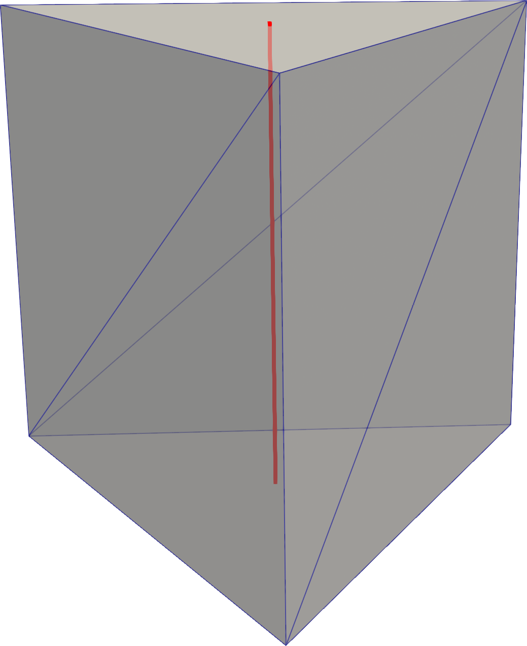
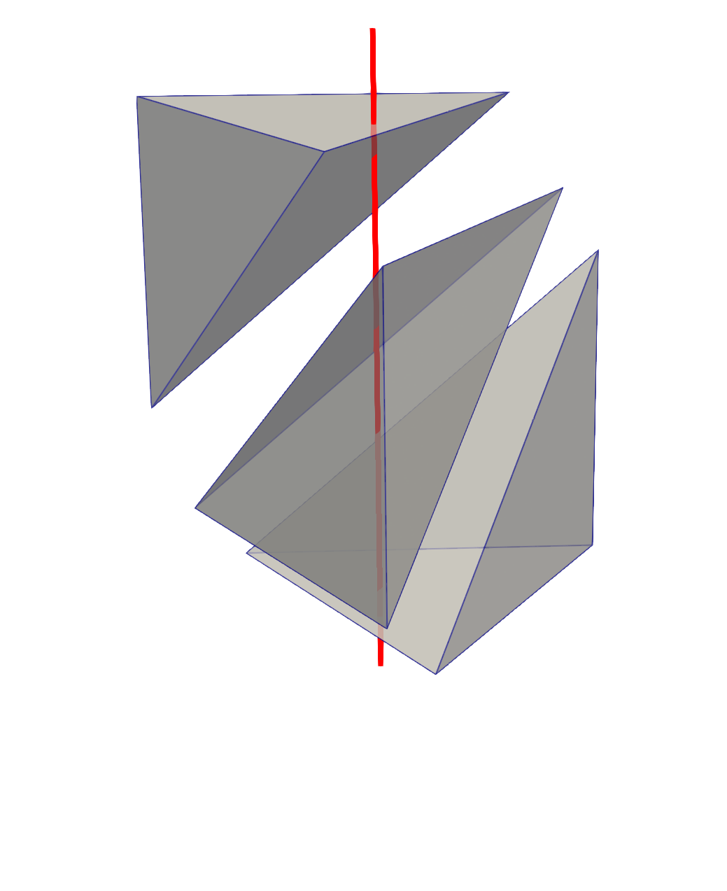
Figure 5: Graphical representation of the domain $\Upsilon$, the liner $\lambda$ in blue and the electrodes $\gamma_{i}$ in red. The different groups of green tetrahedra are associated to each electrodes. On the right, a detail on the construction of cells around an electrode.

Finally, to detect which cell of $\Upsilon$ intersects each electrode segment, we have considered a fast algorithm based on an alternating digital tree (ADT), see [BP91, JFT98] for more details. Once these cells are identified, the maps between them and the intersected electrodes segments are constructed. In general, these are not identity maps.

4 Numerical experiments

The purpose of this section is to validate the proposed approach against laboratory experiments and to study the distribution of current density and electric potential in presence of a highly-resistive liner. We fill a $52[$\mathrm{cm}$]\times 34[$\mathrm{cm}$]\times 40[$\mathrm{cm}$]$ plastic box with different volumes of tap water, whose conductivity is estimated with a Crison MM40+ multimeter to be equal to $\sigma=1/29$ [$\mathrm{S}\text{\,}{\mathrm{m}}^{-1}$].

We deploy a spread of 4 electrodes according to a Wenner-$\alpha$ configuration at the centre of the box along the $x$-axis (Figure 6). The two outer electrodes $C_{1}$ and $C_{2}$ are used to inject the current density with value $\pm\overline{J}_{\Gamma}$, while the two inner ones $P_{1}$ and $P_{2}$ are used to compute the potential difference $\varphi_{\gamma_{2}}-\varphi_{\gamma_{3}}$, the latter being evaluated at the top of the electrodes. The penetration depth of the Wenner-$\alpha$ array for a homogeneous medium can be analytically estimated to be about $0.11L$ or $0.17L$, being $L$ the distance between the current electrodes, either one considers the peak or the median value of the one-dimensional sensitivity function, respectively [RA71, R.D89]. However, the penetration depth of a geoelectrical survey only estimates the depth at which the used array is maximally sensitive and may vary considerably if the investigated medium is heterogeneous.

We set $\Upsilon$ to be completely isolated with null current flow through all the boundaries (i.e., homogeneous Neumann boundary condition) as presented in Problem 4. The domain is discretized with an unstructured mesh with a characteristic length of 5 [$\mathrm{cm}$], which is successively refined to 1 [$\mathrm{cm}$] near the electrodes. No significant improvements are observed in the numerical results considering smaller characteristic lengths.

Figure 6: Wenner-$\alpha$ configuration with four electrodes with spacing $a$.

The electrodes have radius equal to $r=1[$\mathrm{mm}$]$, length of $5[$\mathrm{mm}$]$ and conductivity equal to $\sigma_{\gamma}=1.45\cdot 10^{6}[$\mathrm{S}\text{\,}{\mathrm{m}}^{-1}$]$. The ratio between the radius and the length of the electrodes is larger than what stated previously for convenience in the lab experiments. However, numerical tests with smaller ratios down to 1/100 do not show significant differences. The liner, which will have different shapes for each example, has thickness equal to $\varepsilon=1[$\mathrm{mm}$]$ and conductivity $\sigma_{\lambda}=10^{-9}[$\mathrm{S}\text{\,}{\mathrm{m}}^{-1}$]$. As mentioned before, the liner is approximated as a bi-dimensional object. Contrary to the electrodes, the computational grid is conforming to the liner.

We consider two sets of experiments with increasing level of complexity: in Subsection 4.1 the liner is a horizontal plane, while in Subsection 4.2 the liner has a box shape. The latter mimics the shape of the liner that is placed underneath real landfills to completely isolate the waste body from the surrounding media. In such a case, it is interesting to analyse current and electrical potential distribution according to the position of the electrodes and to the presence of damages in the liner. We will compare the numerical and the experimental values of the estimated apparent resistivity $\rho_{a}$ in [$\mathrm{\SIUnitSymbolOhm}\text{\,}\mathrm{m}$], defined for the Wenner-$\alpha$ configuration as

$$\rho_{a}=2\pi a\frac{\varphi_{\gamma_{2}}-\varphi_{\gamma_{3}}}{i_{\gamma}},$$

where the value of $i_{\gamma}$ is imposed and the difference $\varphi_{\gamma_{2}}-\varphi_{\gamma_{3}}$ comes from measurements or modelling.

4.1 A horizontal liner

In this first test, we want to evaluate the effect of the liner on $\rho_{a}$. The liner is perfectly horizontal and touches all the lateral boundaries of $\Upsilon$. We further assume that $\lambda$ is intact, meaning that neither holes nor defects are present. We consider two settings with different spacing between the electrodes: $a=3[$\mathrm{cm}$]$ and $a=6[$\mathrm{cm}$]$. Since the liner is a highly resistive membrane, it can be approximated with a perfect insulator. In the laboratory test, instead of introducing the liner, we simply decrease the height of the water layer from $h=17[$\mathrm{cm}$]$ to $h=3[$\mathrm{cm}$]$ to ease operations. Following [WT90], as reference value we consider the apparent resistivity $\widetilde{\rho}_{a}$ in [$\mathrm{\SIUnitSymbolOhm}\text{\,}\mathrm{m}$] analytically expressed as

$$\widetilde{\rho}_{a}=\frac{\rho i_{\gamma}}{2\pi}\left(\frac{1}{a}+4\sum_{n=1}^{\infty}\frac{1}{\sqrt{a^{2}+4n^{2}h^{2}}}-\frac{1}{\sqrt{4a^{2}+4n^{2}h^{2}}}\right),$$ (8)

with $\rho=29[$\mathrm{\SIUnitSymbolOhm}\text{\,}\mathrm{m}$]$ being the resistivity of the water. This formula was derived under the condition that $\Upsilon$ is indefinitely laterally extended (i.e., 1D model) and the electrodes are represented as zero-dimensional sources, and, in this work, further simplified since the resistivity of the liner is several orders of magnitude higher than the water resistivity. The instrument used in the laboratory performs several measurements of $\rho_{a}$ for each depth of the liner, so that we can estimate the mean value and the standard deviation, which can be used as proxy for the reliability of the measurements, as reported in Figure 7. In addition, measurement errors were also checked with reciprocal measurements, i.e. switching current and potential electrodes, but values are rather small confirming that the measured $\rho_{a}$ values are reliable.

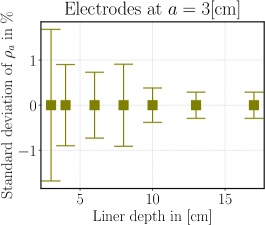
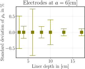
Figure 7: Percentages of standard deviations, centred at their mean value, for the measurements of $\rho_{a}$ for the two experiments, for the example in Subsection 4.1.

In the numerical simulations, we adopt two strategies to account for the liner $\lambda$: i) we consider the entire domain $\Upsilon$ and place a planar surface with very low electric conductivity at a certain depth; ii) since $\lambda$ is highly resistive, we simply remove the part of $\Upsilon$ below the liner and impose a null current density flux condition at the boundary, as schematically shown in Figure 8. Both TPFA and MPFA are considered as discretization schemes. We can thus evaluate the effect of the liner and compare the obtained results with the laboratory experiments.

Figure 8: Schematic representation of the domain of example in Subsection 4.1. The resistive interface of the liner is represented by an interface (left) or by the bottom of the domain (right).

In Figure 9 we show the apparent resistivities obtained in the simulations, in the laboratory experiments, and with the analytical relationship (8). The measured standard deviations (Figure 7) are also represented and now centred in the actual values of the apparent resistivity. Since these standard deviations are rather small they are hardly visible in the graph. All the results show the same trend: by decreasing the liner depth, the apparent resistivity increases because the liner is closer to the electrodes.

We note that the results of the simulations does not change if either $\lambda$ is included in the modelled domain or $\Upsilon$ is reduced accordingly. This means that the laboratory setting is appropriate and can be compared with the simulations when $\lambda$ is considered. Moreover, there is a clear difference between the results obtained from the TPFA and MPFA schemes, having for the former, for $a=3[$\mathrm{cm}$]$, a non-monotone behaviour with respect to the liner depth.

By comparing the synthetic data with the measured ones, we observe that the numerical solutions computed with MPFA are in good agreement, while the TPFA ones are less accurate. A possible explanation is that the latter is not consistent when using simplicial grids and, therefore, the obtained results might not be reliable.

Finally, we observe that, for a spacing of $a=6[$\mathrm{cm}$]$, the measured and computed values of $\rho_{a}$ are higher than the actual one. This can be due to the fact that the considered model is not 1D, thus we could not apply relationship (8).

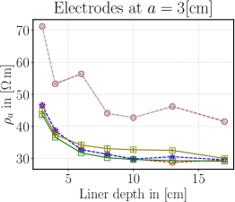
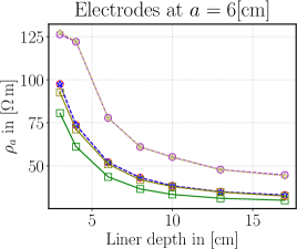
Figure 9: Results for the example in Subsection 4.1. Apparent resistivities computed and measured for several liner depths and for electrode spacing $a=3[$\mathrm{cm}$]$ (left) and $a=6[$\mathrm{cm}$]$ (right).

Figure 10 shows a comparison between the numerical results and the values obtained with (8) when the computational domain $\Upsilon$ is laterally extended to $100\times 100\times 40$ [${\mathrm{cm}}^{3}$]. The results are now in good agreement, confirming that the discrepancy in Figure 9 for $a=6[$\mathrm{cm}$]$ is mainly due to boundary effects. With respect to the values of penetration depth stated before, our tests show that the Wenner-$\alpha$ array becomes insensitive to the resistive liner at depths approximately greater than 3 times the electrode spacing.

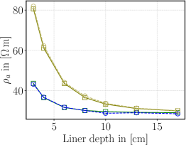
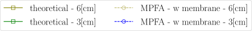
Figure 10: Apparent resistivities computed with MPFA and estimated with relationship (8) for different values of $a$ when the computational domain $\Upsilon$ is laterally extended to $100\times 100\times 40$ [${\mathrm{cm}}^{3}$].

Some of the numerical solutions computed with MPFA are illustrated in Figure 11 with the liner at different depths and for an electrode spacing $a=3[$\mathrm{cm}$]$. The influence of the liner on the electric potential is clearly visible, but becomes less evident when the liner is farther from the electrodes. Below the liner the potential is essentially homogeneous. Figure 12 shows, for the same setting, the current lines with the associate current density, which is injected in $\Upsilon$ from $\gamma_{1}$ and is drawn from $\gamma_{4}$. Again, it is clearly visible how the liner practically confines current circulation in the upper part of the domain only.

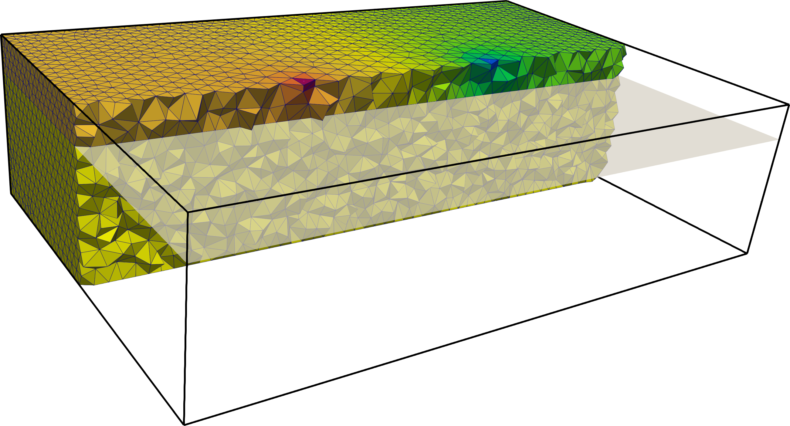
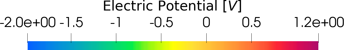
Figure 11: Results for the example in Subsection 4.1. Electric potential in the modelled domain with the liner at depth $h=3[$\mathrm{cm}$]$ (left) and $h=8[$\mathrm{cm}$]$ (right).

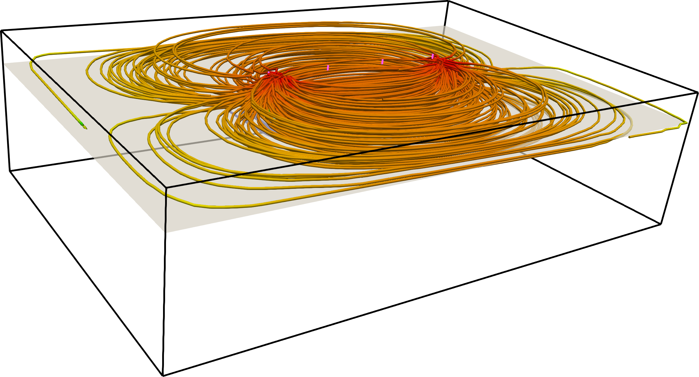
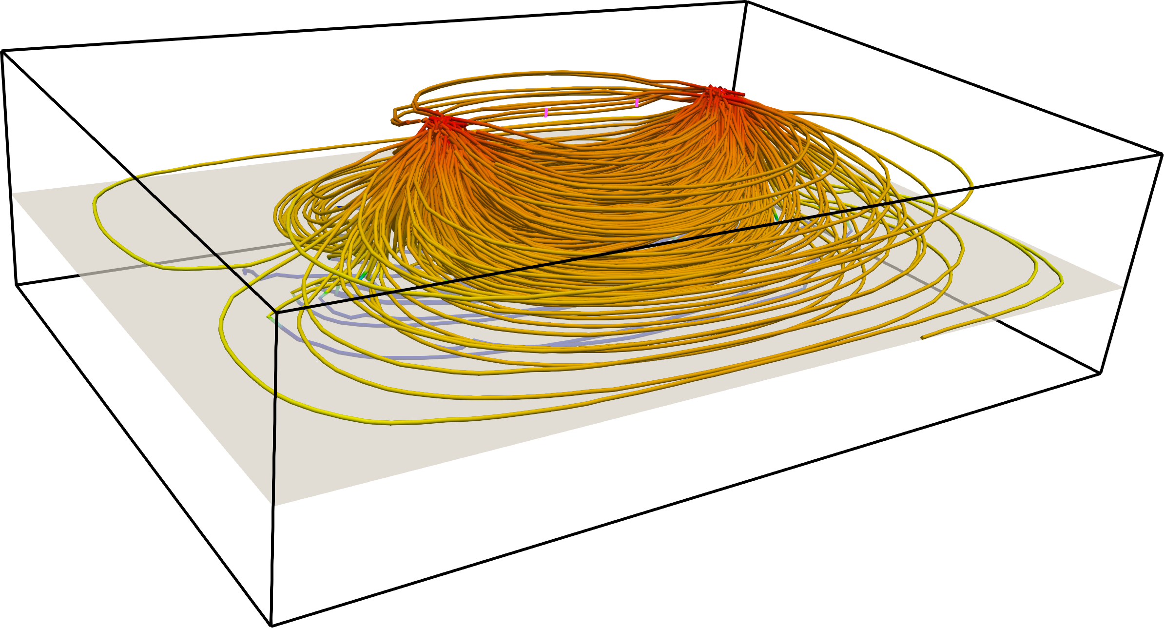
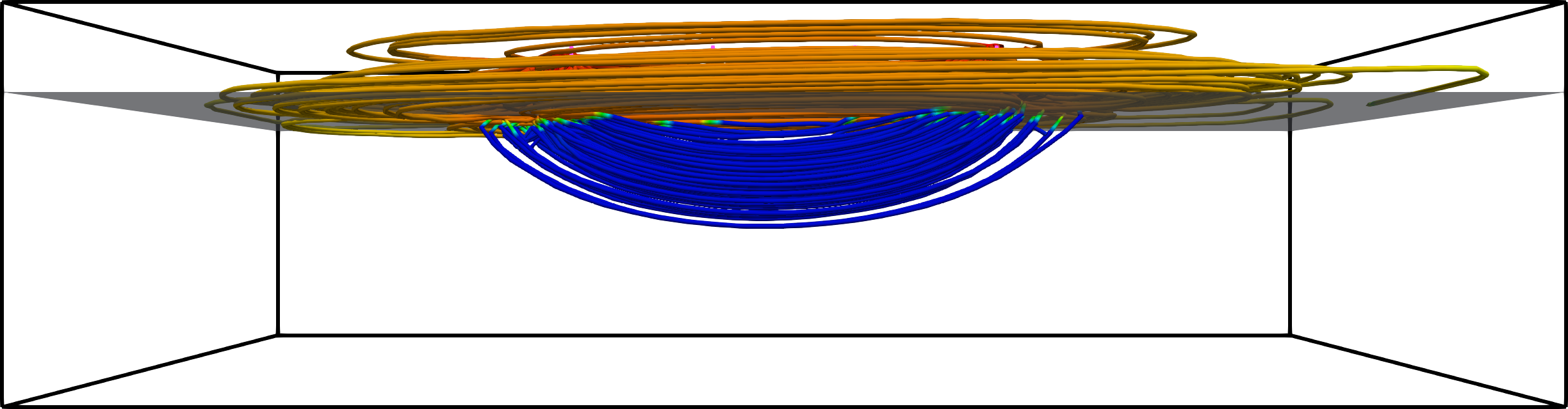
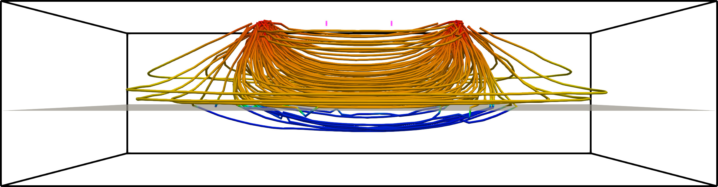
Figure 12: Results for the example in Subsection 4.1. Current lines and the associated current density in the modelled domain with the liner at depth $h=3[$\mathrm{cm}$]$ (left) and $h=8[$\mathrm{cm}$]$ (right).

4.2 A box-shaped liner

In this section we mainly want to evaluate the effect of a hole in the liner and its impact on the resulting apparent resistivity according to different electrode deployments. We consider the liner has a box shape, both with and without a hole $\eta$ in its bottom surface. The box has dimension $20\times 14\times 7.2[${\mathrm{cm}}^{3}$]$ and minimum coordinates in $(20.5,10.5,7.2)[$\mathrm{cm}$]$, the hole has diameter of $0.5[$\mathrm{cm}$]$ and is centred in $(25.5,18.5,7.2)[$\mathrm{cm}$]$ (Figure 13). We consider three deployments for the electrodes in a Wenner-$\alpha$ configuration: case i) all electrodes are within the box with a spacing of $3[$\mathrm{cm}$]$; case ii) just the current electrodes $C_{1}$ is placed outside the box; case iii) both the current electrode $C_{1}$ and the potential electrode $P_{1}$ are placed outside the box. For these last two cases the electrode spacing is set to $6[$\mathrm{cm}$]$. Please note that, for this set of experiments, tap water conductivity is estimated in the lab to be equal to $\sigma=1/24$ [$\mathrm{S}\text{\,}{\mathrm{m}}^{-1}$] and the numerical simulations are performed only with the MPFA scheme. The other parameters of the problem are the same of the previous example. In addition, by taking into account possible uncertainties in the laboratory setup, we perform several simulations with the variation of the water level of $\pm 3[$\mathrm{mm}$]$, the variation of the water resistivity of $\pm 2[$\mathrm{\SIUnitSymbolOhm}\text{\,}\mathrm{m}$]$, the variation of the radius of $\eta$ of $\pm 0.15[$\mathrm{mm}$]$, and the shift of the electrodes along $x$ and $y$, with respect to the box, of $\pm 6[$\mathrm{mm}$]$. Figure 14 shows that, for all the cases, the measured apparent resistivities fall into the range of the modelled values. We point out that the measured standard deviations are always lower than 1% and that, for case ii) and case iii), it was not possible to obtain reliable measurements when there is no hole in the liner.

       

Figure 13: Domains for the example in Subsection 4.2: electrode configurations for case ii (left) and case iii (right). Note the presence of the hole $\eta$ in the bottom surface of the liner. See text for details.

Regarding case i, it is interesting to note that the presence of the hole $\eta$ does not significantly affect the value of the apparent resistivity $\rho_{a}$, which implies that this electrode configuration may not be helpful for detecting defects of the liner. Accordingly, the numerical solutions for this configuration do not show relevant differences either the hole is present or not (Figure 15). The current circulates mostly inside the box-shaped liner, where we observe the variations of the electric potential.

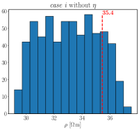
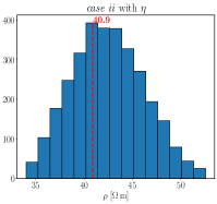
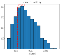
Figure 14: Modelling results for different setups in Subsection 4.2. Histograms of the apparent resistivities modelled by taking into account uncertainties possibly affecting lab setup parameters. Red dashed lines are mean measured resistivities. See text for details.

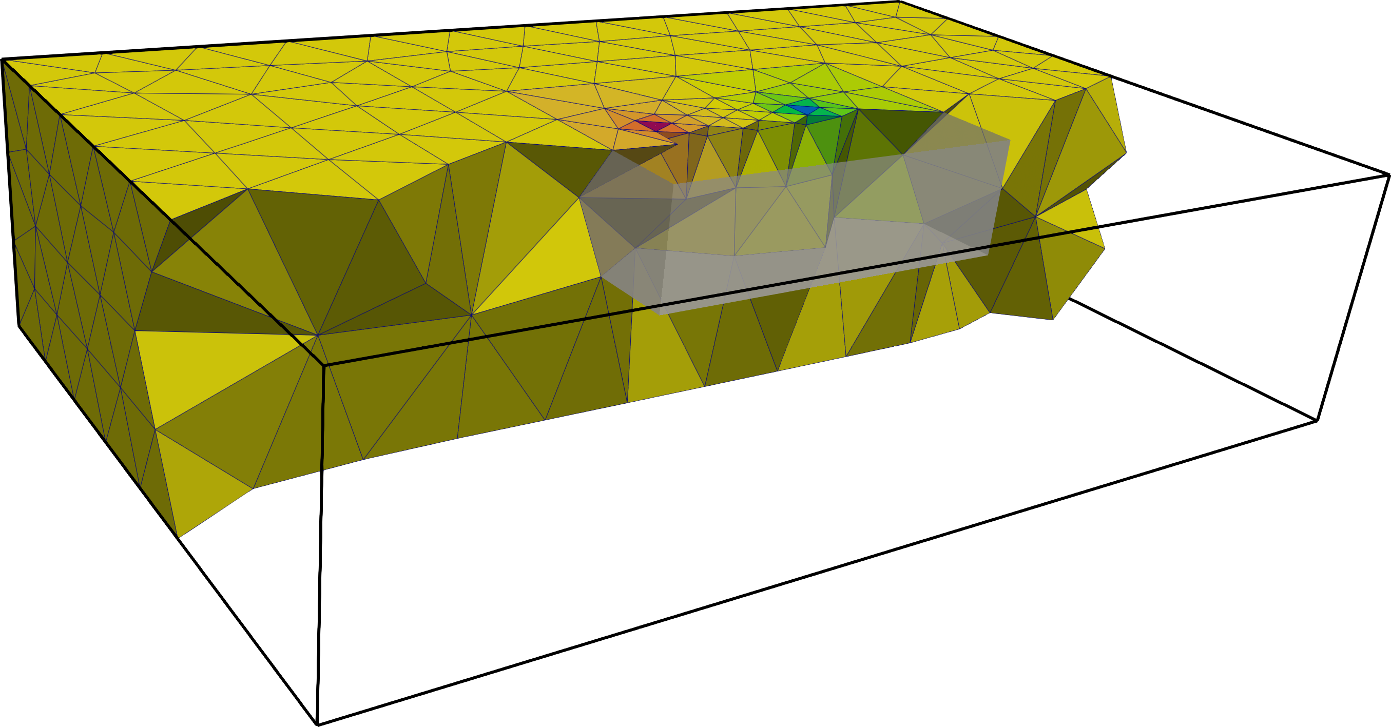
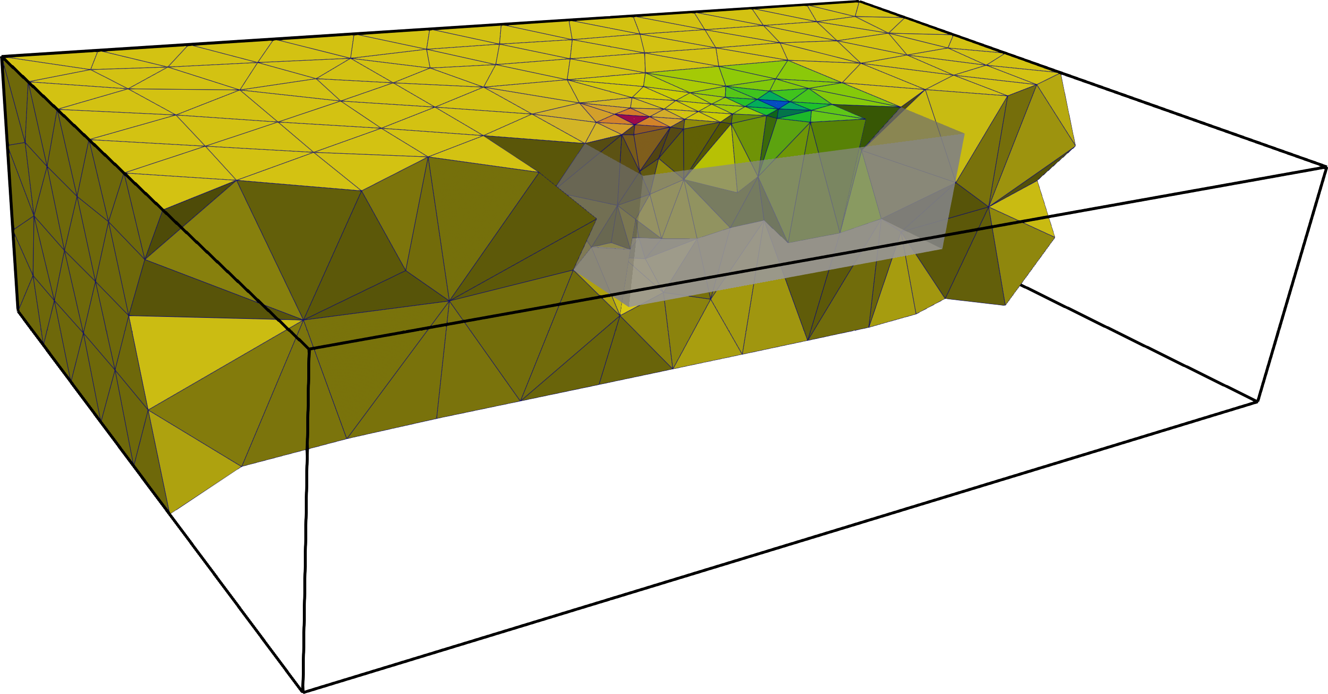
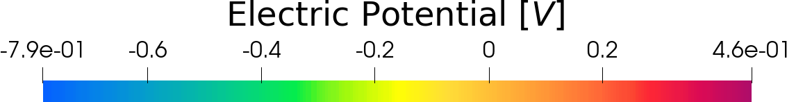
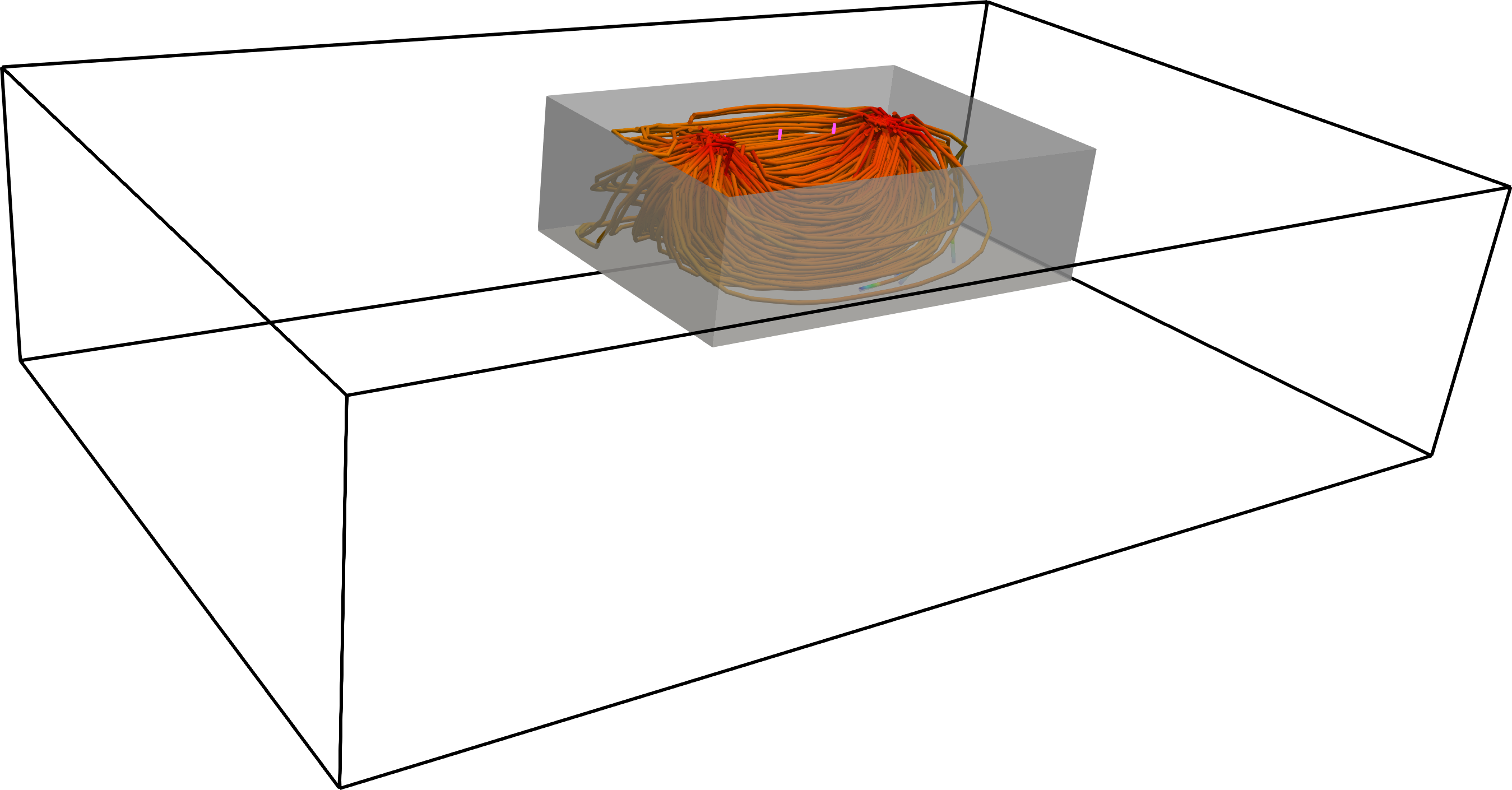
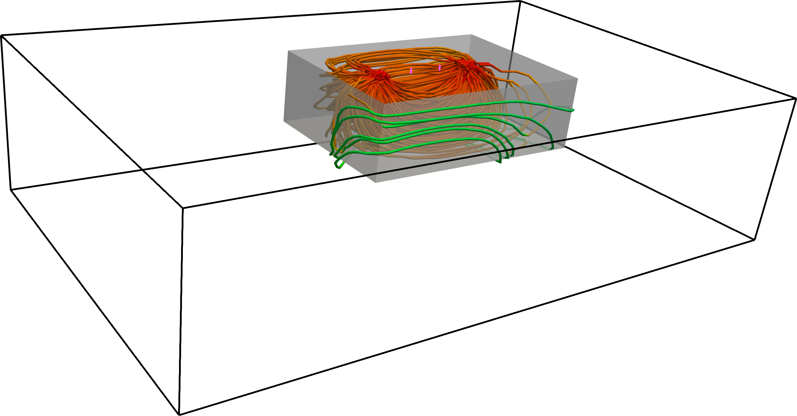
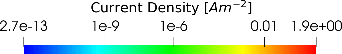
Figure 15: Results for case i described in Subsection 4.2 without (left) and with (right) the hole in the liner. The top and the bottom images show the modelled electric potential and current lines with the associated current density, respectively.

The modelling results for case ii and case iii are similar (Figure 16 and 17), except for the fact that the estimated apparent resitivity is approximately two orders of magnitude higher for the latter (Figure Figure 14). This is due to the presence of the high-resistivity liner between the voltage electrodes in case iii. We generally observe two equi-potential regions, one inside and the other outside the box-shaped liner. When the liner is perforated, the variation of $\varphi$ across $\lambda$ is obviously lower and the main path of the current is from $C_{1}$ to $C_{2}$ through $\eta$. On the contrary, when there is no hole, there in no clear preferential direction for current circulation. For sake of completeness, we report that, for case ii and case iii with no hole, the estimated apparent resitivities are $26.9[$\mathrm{\SIUnitSymbolOhm}\text{\,}\mathrm{m}$]$ and $5.48e10[$\mathrm{\SIUnitSymbolOhm}\text{\,}\mathrm{m}$]$, respectively. Such a large gap between those values is obviously related to the position of both current and voltage electrodes with respect to the liner.

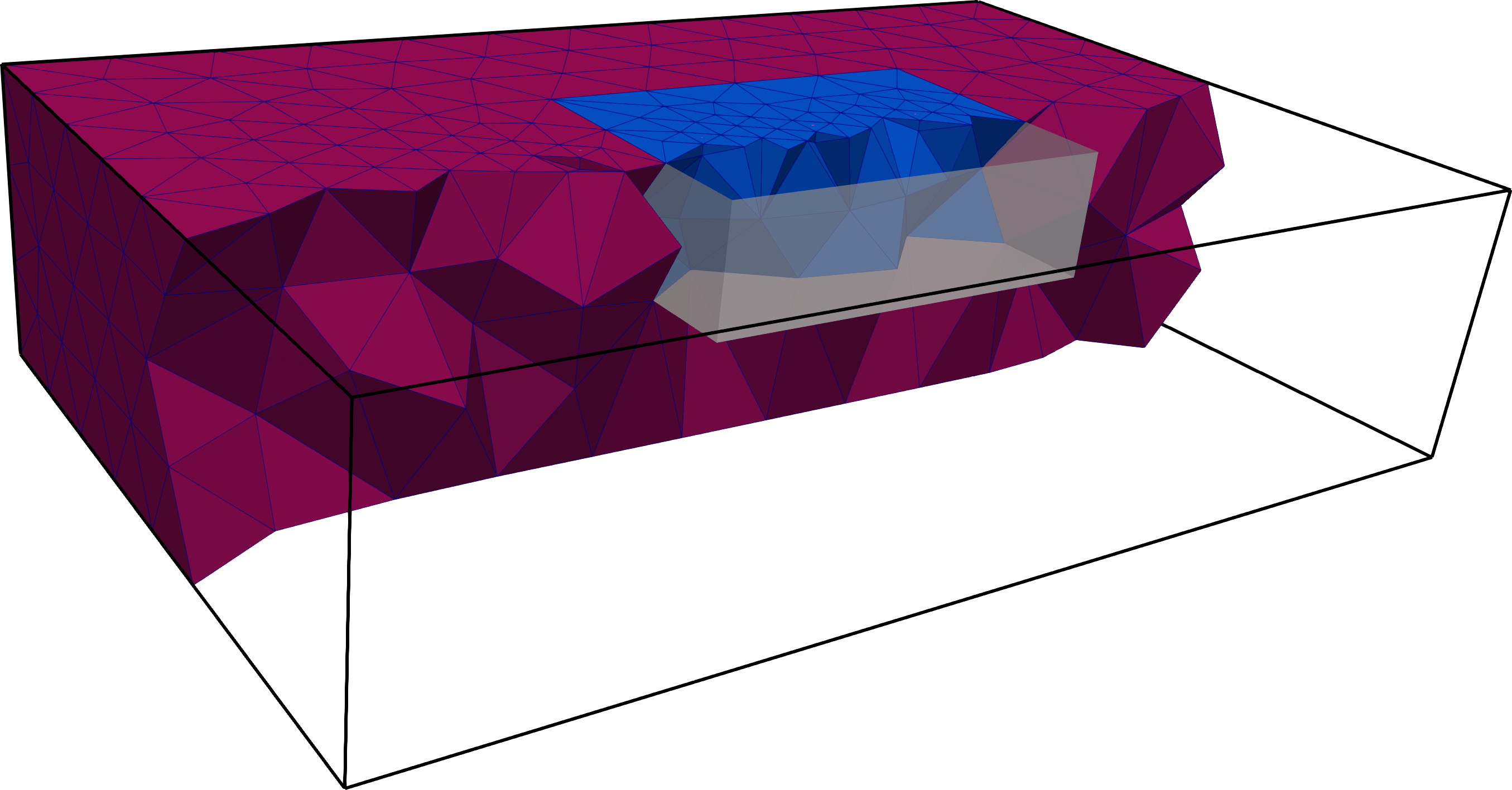
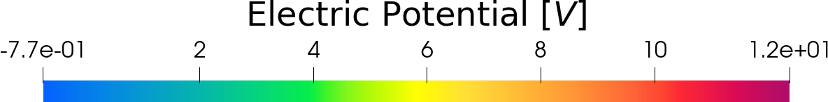
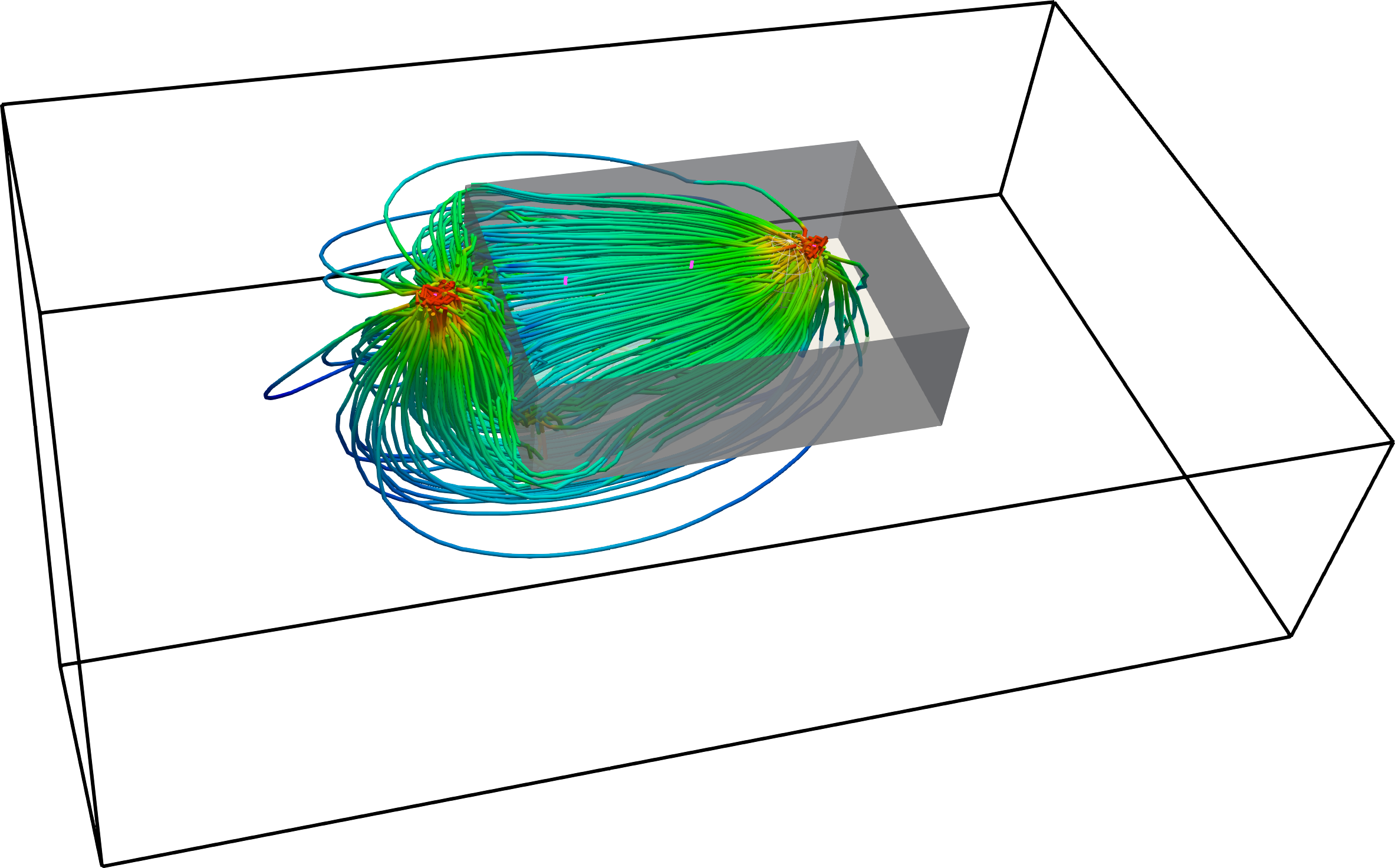
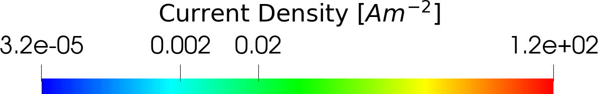
Figure 16: Results for case ii described in Subsection 4.2 without (left) and with (right) the hole in the liner. The top and the bottom images show the modelled electric potential and current lines with the associated current density, respectively. Please note the different colormap ranges for each image.

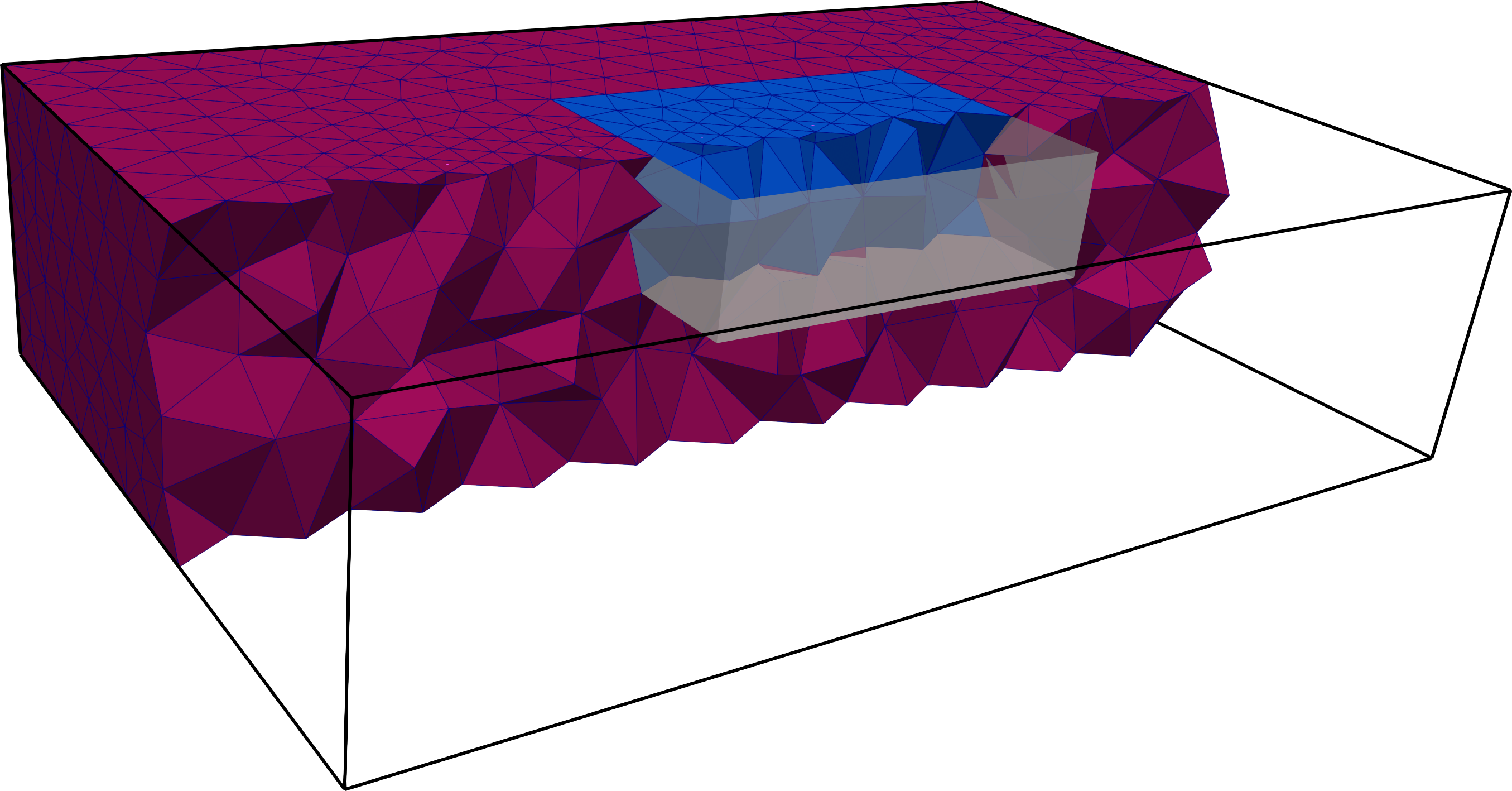
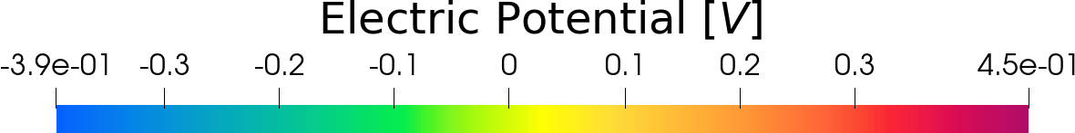
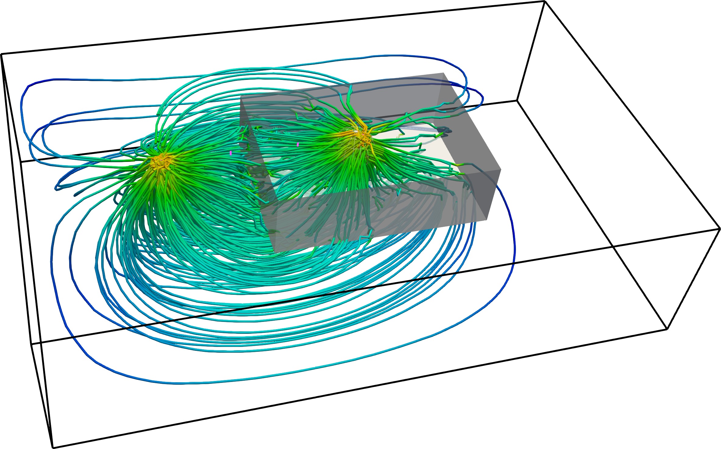
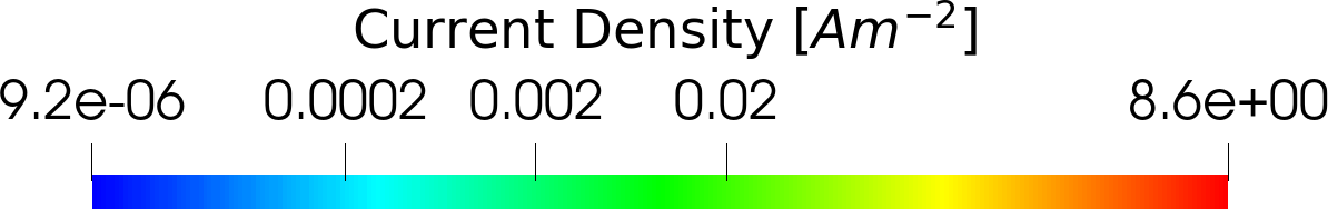
Figure 17: Results for case iii described in Subsection 4.2 without (left) and with (right) the hole in the liner. The top and the bottom images show the modelled electric potential and current lines with the associated current density, respectively. Please note the different colormap ranges for each image.

5 Conclusions

In this work we have presented a mixed-dimensional mathematical model to obtain the electric potential and current density in direct current simulations. The model can handle multiple electrodes and a thin high-resistivity liner included in the domain. These objects have one or two of their dimensions that are very small and thus difficult to be represented exactly by equi-dimensional grids in the simulations. The mixed-dimensional approach used in this work approximates them as object with lower dimension: electrodes as one-dimensional and the liner as two-dimensional objects. New equations have been derived along with new interface conditions to couple the electrodes and the liner with the surrounding domain. To improve the efficiency of the simulation, the electrodes are placed in the background computational grid avoiding an excessive refinement around them. The numerical approximation relies on two cell-centred finite-volume schemes: the two-point and multi-point flux approximations. The mathematical model has been tested against laboratory experiments giving reliable solutions, in particular when the multi-point flux approximation was considered. In the first set of laboratory experiments, we validated the code with an analytical relationship and showed that the liner influences the measured apparent resistivity at depth much higher then the penetration depth of a Wenner-$\alpha$ array. In the second set of experiments, we analyzed the presence of a hole in the liner for different deployments of the electrodes and observed that some configurations are more favourable to detect possible defects. We can conclude that the proposed mixed-dimensional model is a reliable tool for direct current simulations. The model can handle particular features that are very important when dealing with geoelectrical investigations of MSWLFs, where large variations of electrical resistivity can occur in very limited space. The approach we developed could also be exported to other application fields, presenting similar governing equations and peculiarities.

References

- [Aav02] Ivar Aavatsmark. An introduction to multipoint flux approximations for quadrilateral grids. Computational Geosciences, 6:405–432, 2002.
- [Aav07a] Ivar Aavatsmark. Interpretation of a two-point flux stencil for skew parallelogram grids. Computational Geosciences, 11(3):199–206, 2007.
- [Aav07b] Ivar Aavatsmark. Multipoint flux approximation methods for quadrilateral grids. In The 9th International Forum on Reservoir Simulation, Abu Dhabi, pages 9–13, 2007.
- [AFS+21] Alessandro Aguzzoli, Alessio Fumagalli, Anna Scotti, Luigi Zanzi, and Diego Arosio. Inversion of synthetic and measured 3d geoelectrical data to study the geomembrane below a landfill. In 4th Asia Pacific Meeting on Near Surface Geoscience & Engineering, volume 1, pages 1–5. European Association of Geoscientists & Engineers, 2021.
- [AHZA20] A. Aguzzoli, A. Hojat, L. Zanzi, and D. Arosio. Two dimensional ert simulations to check the integrity of geomembranes at the base of landfill bodies. 2020(1):1–5, 2020.
- [BBF+20] Inga Berre, Wietse M. Boon, Bernd Flemisch, Alessio Fumagalli, Dennis Gläser, Eirik Keilegavlen, Anna Scotti, Ivar Stefansson, Alexandru Tatomir, Konstantin Brenner, Samuel Burbulla, Philippe Devloo, Omar Duran, Marco Favino, Julian Hennicker, I-Hsien Lee, Konstantin Lipnikov, Roland Masson, Klaus Mosthaf, Maria Giuseppina Chiara Nestola, Chuen-Fa Ni, Kirill Nikitin, Philipp Schädle, Daniil Svyatskiy, Ruslan Yanbarisov, and Patrick Zulian. Verification benchmarks for single-phase flow in three-dimensional fractured porous media. Advances in Water Resources, 147, 2020.
- [BD03] Andrew Binley and William Daily. The performance of electrical methods for assessing the integrity of geomembrane liners in landfill caps and waste storage ponds. Journal of Environmental and Engineering Geophysics, 8(4):227–237, 2003.
- [BDOH00] C. Bernstone, T. Dahlin, T. Ohlsson, and H. Hogland. Dc-resistivity mapping of internal landfill structures: two pre-excavation surveys. Environmental Geology, 39(3):360–371, Jan 2000.
- [BDR97] Andrew Binley, William Daily, and Abelardo Ramirez. Detecting leaks from environmental barriers using electrical current imaging. Journal of Environmental and Engineering Geophysics, 2(1):11–19, Mar 1997.
- [BGS22] Stefano Berrone, Denise Grappein, and Stefano Scialó. 3d-1d coupling on non conforming meshes via a three-field optimization based domain decomposition. Journal of Computational Physics, 448:110738, 2022.
- [BK05] Andrew Binley and Andreas Kemna. DC Resistivity and Induced Polarization Methods, pages 129–156. Springer Netherlands, Dordrecht, 2005.
- [BP91] Javier Bonet and Jaime Peraire. An alternating digital tree (adt) algorithm for 3d geometric searching and intersection problems. International Journal for Numerical Methods in Engineering, 31(1):1–17, 1991.
- [BSB+20] Guillaume Blanchy, Sina Saneiyan, Jimmy Boyd, Paul McLachlan, and Andrew Binley. Resipy, an intuitive open source software for complex geoelectrical inversion/modeling. Computers & Geosciences, 137:104423, 2020.
- [CLZ19] Daniele Cerroni, Federica Laurino, and Paolo Zunino. Mathematical analysis, finite element approximation and numerical solvers for the interaction of 3d reservoirs with 1d wells. GEM - International Journal on Geomathematics, 10(1):4, Jan 2019.
- [DC17] Giorgio De Donno and Ettore Cardarelli. Tomographic inversion of time-domain resistivity and chargeability data for the investigation of landfills using a priori information. Waste Management, 59:302–315, 2017.
- [DFL+18] R. Di Maio, S. Fais, P. Ligas, E. Piegari, R. Raga, and R. Cossu. 3d geophysical imaging for site-specific characterization plan of an old landfill. Waste Management, 76:629–642, 2018.
- [DPC+13] Lorenzo De Carlo, Maria Teresa Perri, Maria Clementina Caputo, Rita Deiana, Michele Vurro, and Giorgio Cassiani. Characterization of a dismissed landfill via electrical resistivity tomography and mise-á-la-masse method. Journal of Applied Geophysics, 98:1–10, 2013.
- [DQ08] Carlo D’Angelo and Alfio Quarteroni. On the coupling of 1d and 3d diffusion-reaction equations: application to tissue perfusion problems. Mathematical Models and Methods in Applied Sciences, 18(08):1481–1504, 2008.
- [DRL10] T. Dahlin, H. Rosqvist, and V. Leroux. Resistivity-ip mapping for landfill applications. First Break, 28(8), 2010.
- [DS12] Carlo D’Angelo and Anna Scotti. A mixed finite element method for Darcy flow in fractured porous media with non-matching grids. Mathematical Modelling and Numerical Analysis, 46(02):465–489, 2012.
- [FK18] Alessio Fumagalli and Eirik Keilegavlen. Dual virtual element method for discrete fractures networks. SIAM Journal on Scientific Computing, 40(1):B228–B258, 2018.
- [FKS19] Alessio Fumagalli, Eirik Keilegavlen, and Stefano Scialò. Conforming, non-conforming and non-matching discretization couplings in discrete fracture network simulations. Journal of Computational Physics, 376:694–712, 2019.
- [Fra97] William Frangos. Electrical detection of leaks in lined waste disposal ponds. Geophysics, 62(6):1737–1744, 1997.
- [FS20] Alessio Fumagalli and Anna Scotti. A multi-layer reduced model for flow in porous media with a fault and surrounding damage zones. Computational Geosciences, 24(3):1347–1360, 2020.
- [GKN20] Ingeborg Gåseby Gjerde, Kundan Kumar, and Jan Martin Nordbotten. A singularity removal method for coupled 1d–3d flow models. Computational Geosciences, 24(2):443–457, Apr 2020.
- [GKNW19] Ingeborg Gåseby Gjerde, Kundan Kumar, Jan Martin Nordbotten, and Barbara Wohlmuth. Splitting method for elliptic equations with line sources. ESAIM: M2AN, 53(5):1715–1739, 2019.
- [GR09] Christophe Geuzaine and Jean-François Remacle. Gmsh: A 3-d finite element mesh generator with built-in pre- and post-processing facilities. International Journal for Numerical Methods in Engineering, 79(11):1309–1331, 2009.
- [JFT98] Nigel P. Weatherill Joe F. Thompson, Bharat K. Soni, editor. Handbook of Grid Generation. CRC Press, 1998.
- [KBF+20] Eirik Keilegavlen, Runar Berge, Alessio Fumagalli, Michele Starnoni, Ivar Stefansson, Jhabriel Varela, and Inga Berre. Porepy: An open-source software for simulation of multiphysics processes in fractured porous media. Computational Geosciences, 2020.
- [KLMZ21] Miroslav Kuchta, Federica Laurino, Kent-Andre Mardal, and Paolo Zunino. Analysis and approximation of mixed-dimensional pdes on 3d-1d domains coupled with lagrange multipliers. SIAM Journal on Numerical Analysis, 59(1):558–582, 2021.
- [LDR10] V. Leroux, T. Dahlin, and H. Rosqvist. Time-domain ip and resistivity sections measured at four landfills with different contents. Near Surface 2010, P09, 2010.
- [Lok22] Meng Heng Loke. Tutorial : 2-d and 3-d electrical imaging surveys. In Geotomo Software, 2022.
- [LRDC19] M.H. Loke, D. Rucker, T. Dahlin, and J.E. Chambers. Recent advances in the geoelectrical method and new challenges: A software perspective. FastTimes, 24(4):56–62, 2019.
- [LRQ+19] C. Ling, A. Revil, Y. Qi, F. Abdulsamad, P. Shi, S. Nicaise, and L. Peyras. Application of the mise-à-la-masse method to detect the bottom leakage of water reservoirs. Engineering Geology, 261:105272, Nov 2019.
- [Mej00] Maxwell A. Meju. Geoelectrical investigation of old/abandoned, covered landfill sites in urban areas: model development with a genetic diagnosis approach. Journal of Applied Geophysics, 44(2):115–150, 2000.
- [Men18] William Menke. Geophysical Data Analysis: Discrete Inverse Theory. Academic Press, 4th edition, 2018.
- [MJR05] Vincent Martin, Jérôme Jaffré, and Jean Elisabeth Roberts. Modeling Fractures and Barriers as Interfaces for Flow in Porous Media. SIAM J. Sci. Comput., 26(5):1667–1691, 2005.
- [NBFK19] Jan Martin Nordbotten, Wietse Boon, Alessio Fumagalli, and Eirik Keilegavlen. Unified approach to discretization of flow in fractured porous media. Computational Geosciences, 23(2):225–237, 2019.
- [Pea78] Donald W. Peaceman. Interpretation of Well-Block Pressures in Numerical Reservoir Simulation(includes associated paper 6988 ). Society of Petroleum Engineers Journal, 18(03):183–194, 06 1978.
- [Pea83] Donald W. Peaceman. Interpretation of Well-Block Pressures in Numerical Reservoir Simulation With Nonsquare Grid Blocks and Anisotropic Permeability. Society of Petroleum Engineers Journal, 23(03):531–543, 06 1983.
- [RA71] A Roy and A Apparao. Depth of investigation in direct current methods. Geophysics, 36(5):943–959, 1971.
- [R.D89] Barker R.D. Depth of investigation of collinear symmetrical four-electrode arrays. Geophysics, 54:1031–1037, 1989.
- [RG11] Carsten Rücker and Thomas Günther. The simulation of finite ert electrodes using the complete electrode model. GEOPHYSICS, 76(4):F227–F238, 2011.
- [RGW17] Carsten Rücker, Thomas Günther, and Florian M. Wagner. pygimli: An open-source library for modelling and inversion in geophysics. Computers & Geosciences, 109:106–123, 2017.
- [TVFT14] P. Tsourlos, G.N. Vargemezis, I. Fikos, and G.N. Tsokas. Dc geoelectrical methods applied to landfill investigation: case studies from greece. First Break, 32(8), 2014.
- [VSP+11] P. Vaudelet, M. Schmutz, M. Pessel, M. Franceschi, R. Guérin, O. Atteia, A. Blondel, C. Ngomseu, S. Galaup, F. Rejiba, and P. Bégassat. Mapping of contaminant plumes with geoelectrical methods. a case study in urban context. Journal of Applied Geophysics, 75(4):738–751, 2011.
- [WT90] R.E. Sheriff W.M. Telford, L.P. Geldart. Applied Geophysics. Cambridge University Press, 2nd edition, 1990.