Turbulent processes and mean-field dynamo

Abstract

Mean-field dynamo theory has important applications in solar physics and galactic magnetism. We discuss some of the many turbulence effects relevant to the generation of large-scale magnetic fields in the solar convection zone. The mean-field description is then used to illustrate the physics of the $\alpha$ effect, turbulent pumping, turbulent magnetic diffusivity, and other effects on a modern solar dynamo model. We also discuss how turbulence transport coefficients are derived from local simulations of convection and then used in mean-field models.

1 Introduction

The problem of solar and stellar dynamos is still an open one. In spite of tremendous progress over recent decades, we still do not understand with any degree of certainty the reason behind the equatorward migration of solar activity belts, the dependence of cycle frequency on rotation frequency, or the level of magnetic activity. All models of solar and stellar magnetism rely on some assumptions. Even the most realistic simulations suffer from finite resolution and the compromises in the physics that are made. The crucial question is then, when and where we are allowed to make compromises and when not. Among those approximations is the second-order correlation approximation (SOCA), also known as the first-order smoothing approximation. These are nowadays either replaced by other approximations or by numerical techniques such as the test-field method (TFM), as will be explained later in this review.

The Sun’s magnetic field exhibits a clear mean field with spatio-temporal order: antisymmetry of radial and toroidal fields about the equator and the 11-yr cycle. This mean field can well be described by an azimuthal average. The radial component of such an azimuthally averaged mean field has a typical strength of $\pm 10\,{\rm G}$. This is not much compared with the peak strength of $\pm 2\,{\rm kG}$ in sunspots, but much of this is “lost” in the process of averaging. Of course, whatever is lost corresponds to fluctuations, which actually play crucial parts and correlations between different fluctuations lead to various mean-field effects.

Mathematically, once an averaging procedure has been defined, we have the mean field ${\overline{\bm{B}}}$, indicated by an overbar. Then, the difference between the actual and the mean field, $\bm{B}$ and ${\overline{\bm{B}}}$, gives the fluctuating field as $\bm{b}\equiv\bm{B}-{\overline{\bm{B}}}$. The same procedure also applies to all other quantities. This formal distinction between mean and fluctuating fields, which are sometimes also called large-scale and small-scale fields, is important in discussions with observers. Coronal mass ejections, for example, are superficially reported as being part of a large-scale field, but this may not be true anymore when we think of averaging over the full solar circumference. Thus, paradoxically, even if something is large by some standards, it may not qualify as large-scale under this formal definition of an azimuthal average.

Azimuthal averaging is not always a good recipe. Some stars have nonaxisymmetric magnetic fields, and even the Sun is believed to have what is known as active longitudes – a weak nonaxisymmetric magnetic field on top of a predominantly axisymmetric one. Those nonaxisymmetric fields might best be described through low-order Fourier mode filtering. This is probably completely fine, but slightly problematic at the formal level, because then the average of the product of mean and fluctuating fields is no longer vanishing, as it would be in the case of an azimuthal average. This mathematical property is one of several rules that are called the Reynolds rules. However, as alluded to above, the violation of this particular Reynolds rule is probably just a technicality that makes mean-field predictions less accurate. We refer here to the work of Zhou et al (2018) for a detailed investigation. There are a number of other limitations in mean-field theories that will be discussed below.

The purpose of defining mean fields is twofold. On the one hand, they allow us to quantify large-scale magnetic, velocity, and other fields that are observed or that are present in a simulation. On the other hand, they allow us to develop predictive theories for these averages. In these theories, mean fields can sometimes emerge because of instabilities and/or because of suitable boundary conditions. This is possible because of certain mean-field effects, by which one usually means the relations between correlations of fluctuations and various mean fields. Discussing those effects is an important purpose of this review. The ultimate goal of mean-field dynamo theory is to understand and model the Sun and other stars. We therefore also discuss in this review the status of such attempts. For a basic introduction to mean-field theory, which is not the subject of this review, we refer to standard textbooks (Moffatt, 1978; Krause and Rädler, 1980; Zeldovich et al, 1983) and other reviews (Brandenburg and Subramanian, 2005a; Kulsrud and Zweibel, 2008; Miesch and Toomre, 2009; Charbonneau, 2014, 2020; Brandenburg, 2018a; Tobias, 2021; Brandenburg and Ntormousi, 2023; Karak, 2023).

2 The golden years of dynamo theory

The first mean-field model was constructed by Parker (1955). In his model, the toroidal magnetic field is generated from the dipole field by nonuniform rotation. To overcome the restrictions of Cowling’s theorem (Cowling, 1933), Parker suggested that the dipole magnetic field can be regenerated by cyclonic convective motions which transform emerging toroidal magnetic loops into poloidal magnetic field. The coalescing loops can amplify the dipole magnetic field. Studying the combined action of differential rotation and cyclonic motions, he found a solution in the form of a dynamo wave and formulated conditions for the equatorward propagation of dynamo waves. Steenbeck et al (1966) and Steenbeck and Krause (1969) constructed the theoretical basis of mean-field theory, introduced the notion of the mean electromotive force (MEMF) of the turbulence and showed that the Parker effect of the cyclonic convective motions is equivalent to the effective MEMF along the large-scale field. The 1970s can be considered the golden years of mean-field dynamo theory. Back then, Schuessler (1983) stated: “dynamo theory reached the textbook state”, mentioning the famous monographs by Moffatt (1978), Parker (1979), Krause and Rädler (1980), Vainshtein et al (1980), and Zeldovich et al (1983).

Indeed, intensive theoretical and observational studies led to the establishment of the basic solar dynamo scenario, identification of key dynamo parameters, and the formulation of a general paradigm of the nature of solar and stellar magnetism. Schuessler (1983) summarized that mean-field dynamo models can reproduce the “physics of solar activity to a great extent” including:

• Hale’s polarity rule of sunspots groups,

• the time-latitude evolution of sunspot activity (“butterfly diagram”),

• reversals of the polar magnetic field,

• the phase relationship between the evolution of poloidal and toroidal magnetic fields and their consistence with the observed butterfly diagrams (Stix, 1976),

• rigid rotation of the magnetic sector structure and coronal holes (Stix, 1974, 1977),

• chaotic variations of dynamo activity either due to a random $\alpha$ effect or the dynamo nonlinearity from the Lorentz force (Leighton, 1969; Yoshimura, 1978; Ruzmaikin, 1981), and

• a quantitative understanding of the solar torsional oscillations (Schuessler, 1981; Yoshimura, 1981).

We note that the first and second items are based on the assumption that sunspot groups are formed from the large-scale toroidal magnetic field. Already at the time it was recognized that the mean-field models need to take into account the fibril state of the magnetic field which we observed at the solar surface. We return to this point later.

Classical mean-field dynamo models utilize the $\alpha\Omega$ scenario using the differential rotation ($\Omega$ effect) as the source of the toroidal magnetic flux production and the $\alpha$ effect for the poloidal magnetic field generation. Since the seminal work of Pouquet et al (1976), it started to become clear that the magnetic helicity results in an important nonlinear contribution to the $\alpha$ effect and turbulent magnetic field generation (Kleeorin and Ruzmaikin, 1982).

3 Mean-field theory and avoiding some of its limitations

We can never expect a mean-field theory to produce an accurate representation of reality. One reason is the fact that the underlying turbulence has stochastic aspects, so each realization with slightly different initial conditions would result in a somewhat different outcome. However, there could be other reasons for discrepancies that we discuss next. Some of those discrepancies can nowadays be avoided.

3.1 Mean-field electrodynamics

In mean-field theory, one derives evolution equations for the averaged fields, namely the mean magnetic field ${\overline{\bm{B}}}$, the mean velocity $\overline{\bm{U}}$, and the mean thermodynamic variables such as mean specific entropy $\overline{S}$ and the mean density $\overline{\rho}$. Often, one neglects the evolution of $\overline{\bm{U}}$, $\overline{S}$, and $\overline{\rho}$, which is then already an important limitation.

If one focuses on the evolution of the mean magnetic field only, one often talks about the mean-fields electrodynamics or quasi-kinematic mean-field theory, which can still be nonlinear if the various mean-field transport coefficients depend on the mean fields. If they are unaffected, one talks about kinematic mean-field theory, which is linear. Of course, once there is a dynamo, we have an exponentially growing solution, so the magnetic field would grow without limit, i.e., it would not saturate within kinematic mean-field theory. Obviously, a correct mean-field theory must be nonlinear, but even within the realm of linear theory, there are important lessons to be learnt. Below, we discuss the aspects of nonlocality, which were often omitted out of ignorance, but nowadays we know that this is often not possible and this restriction can easily be relaxed.

3.2 Nonlocality

The mean magnetic field is governed by the mean induction equation, which is sometimes also referred to as the mean-field dynamo equation. The most important term here is the mean electromotive force,

$$\overline{\mathbfcal{E}}=\overline{\bm{u}\times\bm{b}},$$ (1)

i.e., the averaged cross product of velocity and magnetic fluctuations. In mean-field electrodynamics, it is often expressed as

$$\overline{\cal E}{}_{i}=\overline{\cal E}{}_{0i}+\alpha_{ij}\overline{B}_{j}+\eta_{ijk}\partial\overline{B}_{j}/\partial x_{k}+...,$$ (2)

where the ellipsis denotes higher derivative terms, of which there should be infinitely many, and there should also be time derivatives. The term $\overline{\cal E}{}_{0i}$ is a contribution that can exist already in the absence of a mean field; see Brandenburg and Rädler (2013) for details and numerical experiments. Including only a finite number of derivatives in Eq. (2) and ignoring time derivatives is another important approximation. In fact, it is usually easier to express $\overline{\mathbfcal{E}}$ as a convolution between an integral kernel and the mean field. Furthermore, it is instructive to split the integral kernel into two pieces and write

$$\overline{\cal E}{}_{i}=\overline{\cal E}{}_{0i}+\hat{\alpha}_{ij}\ast\overline{B}_{j}+\hat{\eta}_{ijk}\ast\partial\overline{B}_{j}/\partial x_{k},$$ (3)

where the asterisks mean a convolution in space and time, and the hats denote integration kernels. In principle, the spatial derivative can be absorbed as being part of the integral kernel, but separating the kernel into $\hat{\alpha}_{ij}$ and $\hat{\eta}_{ijk}$ has conceptual advantages, because they preserve the similarity to Eq. (2). Note also that, unlike Eq. (2), where we allowed for arbitrarily many derivatives, here, we have no other terms, because all even derivatives are already absorbed in $\hat{\alpha}_{ij}$ and all odd derivatives are absorbed in $\hat{\eta}_{ijk}$. Time derivatives can also be absorbed in both of them if the convolution with the kernels is also over time.

For the benefit of better interpretation, both $\alpha_{ij}$ and $\eta_{ijk}$ (and analogously also for $\hat{\alpha}_{ij}$ and $\hat{\eta}_{ijk}$) can be broken down into further pieces. The $\alpha_{ij}$ tensor can be split into a symmetric and an antisymmetric tensor. The latter is characterized by a vector, $\gamma_{i}=-\textstyle{\frac{1}{2}}\epsilon_{ijk}\alpha_{jk}$, which corresponds to a pumping velocity. Having in mind that the magnetic gradient tensor can also be split into symmetric and antisymmetric parts, where the latter is the mean current density, ${\overline{\bm{J}}}$, with $\overline{J}_{i}=-\textstyle{\frac{1}{2}}\epsilon_{ijk}\partial\overline{B}_{j}/\partial x_{k}$, we can separate the rank-3 tensor, $\eta_{ijk}$, into a rank-2 tensor operating only on ${\overline{\bm{J}}}$ and the rest operating on the symmetric part of $\partial\overline{B}_{j}/\partial x_{k}$.

The convolution can only be replaced by a multiplication, as in Eq. (2), if the mean field is constant in time (which is normally never the case!) and if it varies at most linearly in space (which is normally also not the case). We return to this point further below.

3.3 Beyond SOCA and scale separation limits

An important question concerns the calculation of the $\alpha_{ij}$ and $\eta_{ijk}$ coefficients or kernels. A problem arises from the fact that the differential equations for these expressions are nonlinear and therefore hard to solve analytically. A commonly used approximation is SOCA. It neglects triple (and higher) correlations in the evolution equations for the fluctuating velocity and magnetic fields. This closure can be applied when either the magnetic Reynolds number, $\mbox{\rm Re}_{\rm M}$, or the Strouhal number, St, are much smaller than unity. These limits are rather restrictive for astrophysical conditions. For example, the convection zones (CZs) of the Sun and stars are in a turbulent state with huge values of the fluid Reynolds number ($\mbox{\rm Re}\gtrsim 10^{12}$), the magnetic Reynolds number ($\mbox{\rm Re}_{\rm M}\gtrsim 10^{8}$), Rayleigh number ($\mbox{\rm Ra}\gtrsim 10^{20}$), and an extremely low Prandtl number ($\Pr\sim 10^{-4}$–$10^{-7}$); see, e.g., Ossendrijver (2003).

Results of Schrinner et al (2005) showed that SOCA does not work well when $\mbox{\rm Re}_{\rm M}$ exceeds unity and St is not small. There are analytical approaches, e.g., different variants of the so-called $\tau$ approximation (Kleeorin et al, 1996; Field and Blackman, 2002; Brandenburg and Subramanian, 2005a), which can be applied in the high Reynolds number limit. The restrictions inherent to SOCA or the $\tau$ approximation no longer apply when calculating solutions of the underlying differential equations numerically. This is done in the TFM (Schrinner et al, 2005, 2007).

Using a set of mean magnetic fields, the TFM allows one to determine the turbulent transport coefficients for arbitrary velocity fields, provided they can be computed or otherwise represented on the computer. The velocity field can be determined either as a solution of the nonlinear Navier-Stokes equations for a forced turbulent flow or it can be obtained as a results of global convective dynamo (GCD) simulations. To compute $\overline{\mathbfcal{E}}$, the solution for the induction equation for the fluctuating magnetic field is needed as well. The original TFM of Schrinner et al (2005, 2007) adopts the scale-separation assumption. It was shown that the TFM describes the dynamo processes for GCD simulations at moderate Reynolds numbers of around $50$ rather well (Schrinner, 2011; Warnecke et al, 2018; Viviani et al, 2018). The calculations within TFM have some technical restrictions and are currently unable to meet the very high astrophysical limits of $\mbox{\rm Re},\mbox{\rm Re}_{\rm M}>10^{6}$. Nevertheless, the current applications of the TFM concern cases with $\mbox{\rm Re},\mbox{\rm Re}_{\rm M}\gg 1$, which is well beyond the SOCA limits. In recent developments of the TFM, Käpylä et al (2022) took compressibility effects into account. They also studied the effects of the small-scale dynamo on the turbulent electromotive force; see also Rempel et al (2023).

An alternative way of extracting the coefficients of the mean-electromotive force employs a multi-dimensional regression method (Brandenburg and Sokoloff, 2002; Racine et al, 2011; Augustson et al, 2015; Simard et al, 2016). In this approach, instead of solving the equations for the fluctuations in the presence of different mean magnetic fields, as it is done in the TFM, the regression methods try to exploit the form of Eq. (2) for the dynamo-generated large-scale magnetic field. Detailed comparisons of the above method with TFM were done by Warnecke et al (2018). It was found that the TFM gives a more accurate representation of the mean-field coefficients than the multidimensional regression method. We encourage the reader to consult this paper for further details. We return to the problem of extracting turbulent transport coefficients from GCDs in Sect. 7.

The limitations discussed so far are in principle all avoidable: (i) The evolution equations for $\overline{\bm{U}}$, $\overline{S}$, and $\overline{\rho}$ can be (and have been) included (Brandenburg et al, 1992), in addition to that for ${\overline{\bm{B}}}$, but in practice, even this is still an approximation in the sense that the full set of coefficients for the equations is not (or only approximately) known. (ii) The electromotive force can be (and has been) expressed as a convolution, which can most effectively be solved by rewriting the equations as a differential equation, as will be described below. (iii) Numerical solutions can be employed to find specific values for $\alpha_{ij}$ and $\eta_{ijk}$; see Warnecke (2018); Warnecke et al (2021) for doing this for solar simulations using the TFM. It often turns out that analytical closure techniques are very useful as a first orientation and they are often also accurate enough for a qualitatively useful model. In special cases, when a more accurate solution is required, the answer may well be obtained numerically using the TFM. The problem is then only that numerical solutions themselves are limited in just the same way as those for a full numerical solution in the solar and stellar dynamo problems.

Figure 1 shows results for $\tilde{\alpha}(k)$ and $\tilde{\eta}_{\rm t}(k)$ with $\nu/\eta=1$. Both $\tilde{\alpha}$ and $\tilde{\eta}_{\rm t}$ decrease monotonously with increasing $|k|$. The functions $\tilde{\alpha}(k)$ and $\tilde{\eta}_{\rm t}(k)$ are well represented by Lorentzian fits of the form

$$\tilde{\alpha}(k)\approx\frac{\alpha_{0}}{1+(k/k_{\rm f})^{2}}\,,\quad\tilde{\eta}_{\rm t}(k)\approx\frac{\eta_{\rm t0}}{1+(k/2k_{\rm f})^{2}}\,.$$ (4)

Figure 1: Top: Dependences of the normalized $\tilde{\alpha}$ and $\tilde{\eta}_{\rm t}$ on the normalized wavenumber $k/k_{\rm f}$ for isotropic turbulence forced at wavenumbers $k_{\rm f}/k_{1}=5$ with $\mbox{\rm Re}_{\rm M}=10$ (squares) and $k_{\rm f}/k_{1}=10$ with $\mbox{\rm Re}_{\rm M}=3.5$ (triangles), all with $\nu/\eta=1$, using data from Brandenburg et al (2008). The solid lines give the Lorentzian fits (4). Bottom: Normalized integral kernels $\hat{\alpha}$ and $\hat{\eta}_{\rm t}$ versus $k_{\rm f}\zeta$ for isotropic turbulence forced at wavenumbers $k_{\rm f}/k_{1}=5$ with $\mbox{\rm Re}_{\rm M}=10$ (squares) and $k_{\rm f}/k_{1}=10$ with $\mbox{\rm Re}_{\rm M}=3.5$ (triangles), all with $\nu/\eta=1$. The solid lines are defined by (5). Adapted from Brandenburg et al (2008).

Also shown in the lower part of Fig. 1 are the kernels $\hat{\alpha}(\zeta)$ and $\hat{\eta}_{\rm t}(\zeta)$, obtained through Fourier transforms of the Lorentzian fits,

$$\hat{\alpha}(\zeta)\approx\textstyle{\frac{1}{2}}\alpha_{0}k_{\rm f}\exp(-k_{\rm f}|\zeta|)\,,\quad\hat{\eta}_{\rm t}(\zeta)\approx\eta_{\rm t0}k_{\rm f}\exp(-2k_{\rm f}|\zeta|)\,.$$ (5)

We see that the profile of $\hat{\eta}_{\rm t}$ is half as wide as that of $\hat{\alpha}$, but it is not known whether this is a general property. It is important to realize that the suggested mean-field modifications employing the Lorentzian forms of the integral convolution kernels are based on empirical results. Nevertheless, they are much more accurate than the approximation of replacing the kernels by $\delta$ functions, which is done in conventional approaches.

Under suitable conditions, the accuracy of the TFM can be so high that discrepancies become apparent that are solely the result of having made unjustified approximations in the comparison. An example is the memory effect. Comparing the growth rate for a supercritical dynamo with that obtained theoretically from the coefficient obtained from the TFM can give noticeable discrepancies if the memory effect is neglected; see Fig. 1 of Hubbard and Brandenburg (2009). The combined Fourier transformed integral kernel is of the form

$$\tilde{\alpha}(k,\omega)\approx\frac{\alpha_{0}}{1+(k/k_{\rm f})^{2}-{\rm i}\omega\tau}\,,\quad\tilde{\eta}_{\rm t}(k,\omega)\approx\frac{\eta_{\rm t0}}{1+(k/2k_{\rm f})^{2}-{\rm i}\omega\tau}\,,$$ (6)

where $\tau$ is well approximated by the turbulent turnover time. Even for stationary flows, the memory effect can be dramatically important (Rädler et al, 2011).

In practice, it is cumbersome to solve the integral equation in time. However, as alluded to above, it is possible to approximate this integral equation by a differential equation for $\overline{\mathbfcal{E}}$ with respect to space and time $t$ of the form

$$\left(1+\tau\frac{\partial}{\partial t}-\ell^{2}\nabla^{2}\right)\overline{\cal E}{}_{i}=\alpha_{ij}\overline{B}_{j}+\eta_{ijk}\partial\overline{B}_{j}/\partial x_{k}.$$ (7)

This has been done in several papers (Rheinhardt and Brandenburg, 2012; Rheinhardt et al, 2014; Brandenburg and Chatterjee, 2018; Pipin, 2023). We return to this in Sect. 5.3.

3.4 The use of mean-field theory

If mean-field theory cannot reliably be applied to a regime outside that of the direct numerical simulations (DNS), one must ask what is then the use of mean-field theory. The answer lies in the fact that mean-field theory provides us with an excellent diagnostic “tool” for approaching the problem. Particular features of a solution can usually be attributed to particular terms in the mean-field equations. This would then allow us a more informed answer by saying that the main dynamo mechanism is, for example, of $\alpha\Omega$ type, or of a specific type of a shear flow dynamo, for example. Thus, mean-field theory may be regarded as a convenient tool for understanding what is going on rather than predicting what might be going on.

4 The catastrophic quenching problem

Since the 1990s, a problem emerged in that numerical dynamo solutions were found to depend on the value of the microphysical magnetic diffusivity. Typically, the strength of the mean-fields then decreases with increasing magnetic Reynolds number. This is unusual and does not have any correspondence with ordinary hydrodynamics where the large-scale dynamics is usually already captured at moderate fluid Reynolds numbers. In its original form, the catastrophic quenching problem refers to the finding that the volume-averaged electromotive force scales with the microphysical magnetic diffusivity, and thus goes to zero when $\eta\to 0$. To some extent, this is a problem related to the use of periodic boundary conditions. However, even for astrophysically more realistic boundary conditions, numerical simulations reveal that there is still a problem. Plasma relaxation experiments have identified the role of magnetic helicity as the main culprit in causing $\eta$-dependent large-scale dynamics and catastrophic quenching. We therefore begin by briefly reviewing the essential findings.

4.1 Lessons from plasma relaxation experiments

The magnetic field is divergence-free and can therefore be written as $\bm{B}={\bm{\nabla}}\times\bm{A}$, where $\bm{A}$ is the magnetic vector potential. The magnetic helicity density is defined as $\bm{A}\cdot\bm{B}$. Its evolution equation follows directly from the uncurled induction equation, $\partial\bm{A}/\partial t=-\bm{E}-{\bm{\nabla}}\Phi$, or, using Ohm’s law, $-\bm{E}=\bm{U}\times\bm{B}-\eta\mu_{0}\bm{J}$, so

$$\frac{\partial\bm{A}}{\partial t}=\bm{U}\times\bm{B}-\eta\mu_{0}\bm{J}-{\bm{\nabla}}\Phi.$$ (8)

It yields the evolution equation for the magnetic helicity density,

$$\frac{\partial}{\partial t}\left(\bm{A}\cdot\bm{B}\right)=-2\eta\mu_{0}\,\bm{J}\cdot\bm{B}-{\bm{\nabla}}\cdot\left(\bm{E}\times\bm{A}+\Phi\bm{B}\right).$$ (9)

It must here be emphasized that there is an important difference to the equation for the magnetic energy density,

$$\frac{\partial}{\partial t}\left(\bm{B}^{2}/2\mu_{0}\right)=-\bm{U}\cdot(\bm{J}\times\bm{B})-2\eta\mu_{0}\,\bm{J}^{2}-{\bm{\nabla}}\cdot\left(\bm{E}\times\bm{B}/\mu_{0}\right).$$ (10)

While both Eqs. (9) and (10) have analogous terms such as dissipation $\propto\bm{J}\cdot\bm{B}$ versus $\propto\bm{J}^{2}$, respectively, and flux terms $\bm{E}\times\bm{A}$ versus Poynting vector $\bm{E}\times\bm{B}/\mu_{0}$, respectively, there is the work against the Lorentz force, $-\bm{U}\cdot(\bm{J}\times\bm{B})$ in Eq. (10), which would be $\bm{U}\cdot(\bm{B}\times\bm{B})$ in Eq. (9), but it obviously vanishes. In statistical equilibrium, $\langle 2\eta\mu_{0}\,\bm{J}^{2}\rangle$ must balance $-\langle\bm{U}\cdot(\bm{J}\times\bm{B})\rangle$, which implies that the current density diverges like $|\bm{J}|\sim\eta^{-1/2}$. By contrast, no magnetic helicity is being produced, and also its dissipation converges to zero like $\propto\eta|\bm{J}\cdot\bm{B}|\to\eta^{1/2}$ as $\eta\to 0$.

Already since the 1970s, we know of the conjecture of J. B. Taylor (1974, 1986) that the magnetic field relaxes under the constraint of magnetic helicity conservation to a nearly force-free field to minimize dissipation. The approximate conservation of magnetic helicity has been verified experimentally in plasma relaxation experiments; see, e.g., Ji et al (1995). There are obviously some differences between the solar convection zone and laboratory plasmas, for example, the role of the electron pressure in the generalized Ohm’s law could play an important role in explaining why magnetic helicity changes are observed to be faster in plasma experiments than what is predicted by Ohm’s law (Ji et al, 1995). Furthermore, the $\alpha$ effect has been identified as the main agent for converting magnetic helicity from the turbulent field to the mean field (Ji, 1999).

In the context of plasma relaxation experiments, it is useful to distinguish between electromagnetic and electrostatic turbulence. This distinction refers to the curl-free and divergence-free parts of the electric field written as $\bm{E}=-{\bm{\nabla}}\Phi-\partial\bm{A}/\partial t$. In plasma relaxation experiments, turbulence is mostly electrostatic. It can be affected by the electron pressure gradient $(en_{\rm e})^{-1}{\bm{\nabla}}p_{\rm e}$ in the generalized Ohm’s law, where $e$ is the unit charge, and $n_{\rm e}$ and $p_{\rm e}$ are the electron density and electron pressure, respectively; see Ji (1999) for details. This leads to a battery term $\propto{\bm{\nabla}}n_{\rm e}\times{\bm{\nabla}}p_{\rm e}$ in the equation for $\partial\bm{B}/\partial t$ and to a magnetic helicity flux, which transports magnetic helicity across physical space, as opposed to wavenumber space (Ji, 1999).

There is the possibility that the divergence of a magnetic helicity flux, $\overline{\mathbfcal{F}}_{\rm f}$, itself can constitute an $\alpha$ effect. This corresponds to $\alpha=-\textstyle{\frac{1}{2}}\bm{B}^{-2}{\bm{\nabla}}\cdot\overline{\mathbfcal{F}}_{\rm f}$; see Vishniac and Cho (2001), who have derived a specific form for such a flux. The subscript ‘f’ indicates that the flux originates from correlations of the fluctuating magnetic field. Mean-field models of the type described below have shown that a dynamo can operate even without kinetic helicity, i.e., it is based only on shear and current helicity fluxes, provided a nondimensional scaling factor in front of the magnetic helicity flux exceeds a certain critical value (Brandenburg and Subramanian, 2005c). However, there are so far no DNS that have supported this kind of behavior, nor has the proposed flux been confirmed (Hubbard and Brandenburg, 2012). Nevertheless, the idea of an $\alpha$ effect being related to the magnetic helicity flux divergence is certainly consistent with the laboratory experiment presented in Fig. 1 of Ji (1999).

The $\alpha$ effect reflects the physics of the inverse cascade of magnetic helicity (Pouquet et al, 1976). In the absence of energy input, this is known to lead to a slower turbulent decay of magnetic energy $\propto t^{-2/3}$ (Hatori, 1984; Biskamp and Müller, 1999). In hydrodynamics, by comparison, the kinetic energy density decays like $t^{-10/7}$ or $t^{-6/5}$, depending on the initial subinertial range energy spectrum (Davidson, 2000); see also Brandenburg and Larsson (2023) for a comparison with the magnetic case.

In the presence of magnetic driving by applying a voltage drop along the magnetic field, small-scale instabilities such as the tearing instability develop. This leads to a sawtooth-like time dependence in the mean toroidal magnetic flux; see Ji and Prager (2002) for a review. This can be associated with the resulting development of a mean electromotive force, $\overline{\mathbfcal{E}}=\overline{\bm{u}\times\bm{b}}$, along with an $\alpha$ effect that accomplishes the helicity transport (Ji, 1999).

Unlike astrophysical dynamos, which are generally understood as self-excited ones, the plasma experiments operate in a regime where a magnetic field is always present, but it is then redistributed by the $\alpha$ effect. The conceptional similarities and differences have been discussed in detail by Blackman and Ji (2006). In the following, we discuss in more detail the consequences imposed by magnetic helicity evolution in astrophysical dynamos. It is important to emphasize, however, that the same physics that is used to explain the catastrophic quenching phenomenology also applies to plasma experiments such as the reversed field pinch, as was shown in corresponding mean-field simulations by Kemel et al (2011).

4.2 Mean fields in periodic domains

Under astrophysical conditions of interest, $\eta$ is so small that the volume-averaged electromotive force would be negligibly small. If this result was actually astrophysically relevant, it would be a “catastrophe,” i.e., it would not be possible to understand astrophysical magnetic fields as mean-field dynamos. The solution to this particular problem turned out to be that relating the volume-averaged electromotive force to the volume-averaged mean magnetic field is only of limited relevance to the problem of $\alpha$ effect dynamos. Any dynamo would produce a non-uniform field. Especially in a periodic domain, the mean magnetic flux through any of the faces of the periodic domain is constant in time, so if it was zero to begin with, it would always remain zero. A dynamo problem can therefore not be formulated in that case.

A proper dynamo problem should always allow for the possibility of the magnetic field to decay to zero if there is sufficient magnetic diffusivity. Simple examples of nontrivial mean fields in a periodic domain are Beltrami fields of the form

$${\overline{\bm{B}}}(x)\propto\begin{pmatrix}0\\ \sin kx\\ \cos kx\end{pmatrix},\quad{\overline{\bm{B}}}(y)\propto\begin{pmatrix}\cos ky\\ 0\\ \sin ky\end{pmatrix},\quad\mbox{or}\quad{\overline{\bm{B}}}(z)\propto\begin{pmatrix}\sin kz\\ \cos kz\\ 0\end{pmatrix},$$ (11)

which can be solutions of the simple $\alpha^{2}$ dynamo problem, $\partial{\overline{\bm{B}}}/\partial t=\alpha{\bm{\nabla}}\times{\overline{\bm{B}}}+\eta_{\rm T}\nabla^{2}{\overline{\bm{B}}}$. Nevertheless, there is still a problem of catastrophic nature because it turned out that the time required to reach the final solution scales inversely with $\eta$. This is demonstrated in Fig. 2, where we show the evolution of one of the three planar averages. In the beginning, all three mean fields grow in a similar fashion, but at some point, only one of the three reaches a significant amplitude. Note, however, that the ultimate saturation takes a resistive time, $\tau_{\rm res}=1/(2\eta k_{1}^{2})$.

4.3 Quenching phenomenology

To understand the reason for the catastrophically slow saturation, it suffices to consider Eq. (9) for the magnetic helicity density. For periodic domains, we just have

$$\frac{{\rm d}{}}{{\rm d}{}t}\langle\bm{A}\cdot\bm{B}\rangle=-2\eta\mu_{0}\langle\bm{J}\cdot\bm{B}\rangle.$$ (12)

This equation is gauge-independent, because the gauge transformation $\bm{A}\to\bm{A}^{\prime}+{\bm{\nabla}}\Lambda$ yields $\langle\bm{A}\cdot\bm{B}\rangle=\langle\bm{A}^{\prime}\cdot\bm{B}\rangle$, with $\langle\bm{B}\cdot{\bm{\nabla}}\Lambda\rangle=\langle{\bm{\nabla}}\cdot(\Lambda\bm{B})\rangle-\langle\Lambda{\bm{\nabla}}\cdot\bm{B}\rangle=0$, using ${\bm{\nabla}}\cdot\bm{B}=0$ and the fact that the domain is periodic, so the average of a divergence vanishes. In numerical calculations, it is often convenient to adopt the Weyl gauge, which implies that $\partial\bm{A}/\partial t=-\bm{E}$, i.e., the scalar potential term drops out.

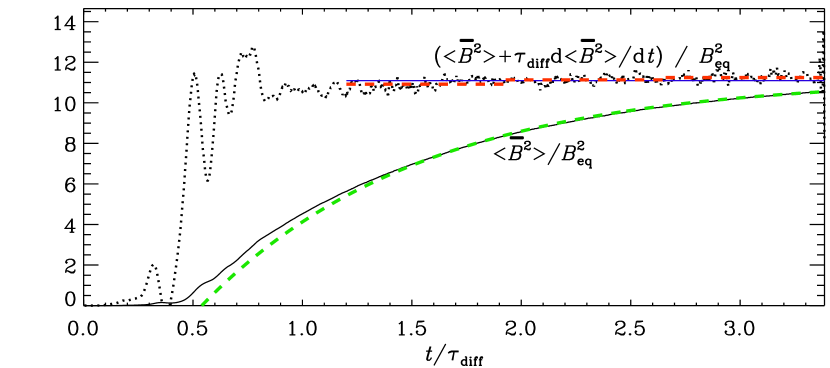
Figure 2: Evolution of the normalized $\langle{\overline{\bm{B}}}^{2}\rangle$ and that of $\langle{\overline{\bm{B}}}^{2}\rangle+\tau_{\rm diff}{\rm d}{}\langle{\overline{\bm{B}}}^{2}\rangle/{\rm d}{}t$ (dotted), compared with its average in the interval $1.2\leq t/\tau_{\rm diff}\leq 3.5$ (horizontal blue solid line), as well as averages over three subintervals (horizontal red dashed lines). The green dashed line corresponds to Eq. (14) with $t_{\rm sat}/\tau_{\rm diff}=0.54$. Adapted from Candelaresi and Brandenburg (2013).

For fully helical large-scale and small-scale magnetic fields of opposite magnetic helicity, Eq. (12) becomes (Brandenburg, 2001)

$${{\rm d}{}\over{\rm d}{}t}\langle{\overline{\bm{B}}}^{2}\rangle=2\eta k_{1}k_{\rm f}B_{\rm eq}^{2}-2\eta k_{1}^{2}\langle{\overline{\bm{B}}}^{2}\rangle,$$ (13)

with the solution

$$\langle{\overline{\bm{B}}}^{2}\rangle=B_{\rm eq}^{2}{k_{\rm f}\over k_{1}}\left[1-e^{-2\eta k_{1}^{2}(t-t_{\rm sat})}\right].$$ (14)

This agrees with the slow saturation behavior seen first in the simulations of Brandenburg (2001); see Fig. 2. Here, $t_{\rm sat}$ is the time when the slow saturation phase commences; see the crossing of the green dashed line with the abscissa. Interestingly, instead of waiting until full saturation is accomplished, one can obtain the saturation value already much earlier simply by differentiating the simulation data to compute (Candelaresi and Brandenburg, 2013)

$$B_{\rm sat}^{2}\approx\langle{\overline{\bm{B}}}^{2}\rangle+\tau_{\rm res}{{\rm d}{}\over{\rm d}{}t}\langle{\overline{\bm{B}}}^{2}\rangle.$$ (15)

Since $\tau_{\rm res}$ involves the microphysical magnetic diffusivity, the quenching is still in that sense catastrophic.

4.4 The $\alpha$ quenching formula

A more complete description is in terms of kinetic and magnetic $\alpha$ effects, i.e.,

$$\alpha=\alpha_{\rm K}+\alpha_{\rm M}\approx-\frac{\tau}{3}\left(\overline{\bm{\omega}\cdot\bm{u}}-\overline{\bm{j}\cdot\bm{b}}/\overline{\rho}\right),$$ (16)

and observing the fact that the magnetic helicity evolution of averages and fluctuations is given by

$$\frac{{\rm d}{}}{{\rm d}{}t}\langle{\overline{\bm{A}}}\cdot{\overline{\bm{B}}}\rangle=+2\langle\overline{\mathbfcal{E}}\cdot{\overline{\bm{B}}}\rangle-2\eta\mu_{0}\,\langle{\overline{\bm{J}}}\cdot{\overline{\bm{B}}}\rangle,$$ (17)

$$\frac{{\rm d}{}}{{\rm d}{}t}\langle\bm{a}\cdot\bm{b}\rangle=-2\langle\overline{\mathbfcal{E}}\cdot{\overline{\bm{B}}}\rangle-2\eta\mu_{0}\,\langle\bm{j}\cdot\bm{b}\rangle.$$ (18)

Equation (17) allows for the possibility that magnetic helicity can be produced by the mean electromotive force, because, in general, $\overline{\mathbfcal{E}}\cdot{\overline{\bm{B}}}\equiv\overline{\bm{u}\times\bm{B}}\cdot{\overline{\bm{B}}}\neq 0$. (By contrast, of course, $(\bm{u}\times{\overline{\bm{B}}})\cdot{\overline{\bm{B}}}=0$.) In particular, if $\overline{\mathbfcal{E}}=\alpha{\overline{\bm{B}}}-\eta_{\rm t}\mu_{0}{\overline{\bm{J}}}$, then, $\overline{\mathbfcal{E}}\cdot{\overline{\bm{B}}}=\alpha{\overline{\bm{B}}}^{2}-\eta_{\rm t}\mu_{0}{\overline{\bm{J}}}\cdot{\overline{\bm{B}}}$, which produces positive (negative) magnetic helicity of the mean field when $\alpha>0$ ($\alpha<0$)

Equation (18) is constructed such that the sum of Eqs. (17) and (18) yields Eq. (12). Given that $\langle\bm{a}\cdot\bm{b}\rangle$ is related to $\langle\bm{j}\cdot\bm{b}\rangle$, which, in turn, is related to a magnetic contribution to the $\alpha$ effect (Pouquet et al, 1976), Eq. (18) can be rewritten as an evolution equation for the total $\alpha$ (Brandenburg, 2008),

$$\frac{{\rm d}{}\alpha_{\rm M}}{{\rm d}{}t}=-2\eta_{\rm t0}k_{\rm f}^{2}\left(\frac{\alpha{\overline{\bm{B}}}^{2}-\eta_{\rm t}\mu_{0}{\overline{\bm{J}}}\cdot{\overline{\bm{B}}}}{B_{\rm eq}^{2}}+\frac{\alpha_{\rm M}}{\mbox{\rm Re}_{\rm M}}\right),$$ (19)

which can also be expressed in the form

$$\alpha({\overline{\bm{B}}})=\frac{\alpha_{0}+\mbox{\rm Re}_{\rm M}\times\mbox{``extra terms''}}{1+\mbox{\rm Re}_{\rm M}{\overline{\bm{B}}}^{2}/B_{\rm eq}^{2}}$$ (20)

where

$$\mbox{``extra terms''}=\eta_{\rm t}\frac{\mu_{0}{\overline{\bm{J}}}\cdot{\overline{\bm{B}}}}{B_{\rm eq}^{2}}-\frac{{\bm{\nabla}}\cdot\overline{\mathbfcal{F}}_{\rm f}}{2k_{\rm f}^{2}B_{\rm eq}^{2}}-\frac{\partial\alpha/\partial t}{2k_{\rm f}^{2}B_{\rm eq}^{2}}.$$ (21)

Note that the last term is here a time derivative. Equation (20) resembles the catastrophic quenching formula of Vainshtein and Cattaneo (1992), but it also shows that it needs to be extended in several important ways: when the mean field is no longer defined as a volume average, extra terms emerge that are of the same order as those in the denominator. They can therefore potentially offset the catastrophic quenching. In practice, this is only partially true, because there are also other terms, for example the aforementioned time derivative term. It is responsible for the fact that a strong field state is only reached after a resistively long time.

4.5 Magnetic helicity fluxes and helicity reversals

Magnetic helicity fluxes could in principle remove the catastrophic quenching problem, but only if preferentially small-scale magnetic helicity is being removed (Kleeorin et al, 2000). To see this, let us first consider the problem of an $\alpha^{2}$ dynamo in insulating boundaries using the Weyl gauge, i.e.,

$$\frac{\partial}{\partial t}{\overline{\bm{A}}}=\alpha{\overline{\bm{B}}}-\eta_{\rm T}\mu_{0}{\overline{\bm{J}}},\quad\mbox{with \; $\partial_{z}\overline{A}_{x}=\partial_{z}\overline{A}_{y}=\overline{A}_{z}=0$}.$$ (22)

The boundary condition implies that $\overline{B}_{x}=\overline{B}_{y}=0$, and is therefore also referred to as the vertical field condition. In this 1-D problem, however, this boundary condition is equivalent to a proper vacuum boundary condition.

The $\alpha^{2}$ dynamo with this boundary condition was first considered by Gruzinov and Diamond (1994), who found that the saturation field strength of such a dynamo decreases with $\mbox{\rm Re}_{\rm M}$. This was later confirmed by Brandenburg and Dobler (2001). In Fig. 3, we show the profiles of magnetic helicity, current helicity, and the magnetic helicity fluxes for Runs A of Brandenburg (2018b) with $\mbox{\rm Re}_{\rm M}=180$. The computational domain is $0\leq z\leq\pi/2$ with a perfect conductor boundary condition on $z=0$ and a vertical field condition on $z=\pi/2$; see Brandenburg (2017) for the relevant mean-field models. For normalization purposes, he defined the reference values

$$C_{\rm f0}=k_{\rm f}B_{\rm eq}^{2}\quad\mbox{and}\quad F_{\rm m0}=\eta_{\rm t0}k_{1}^{2}\int_{0}^{\pi/2}{\overline{\bm{B}}}^{2}\,{\rm d}{}z.$$ (23)

He emphasized that the largest contribution to the magnetic helicity density comes from the large-scale field. Near the surface ($z=\pi/2$), the (negative) magnetic helicity flux from small-scale fields is only about $0.02\,F_{\rm m0}$, which explains why they are not efficient enough to alleviate the catastrophic dependence of the resulting mean magnetic field (Del Sordo et al, 2013; Rincon, 2021).

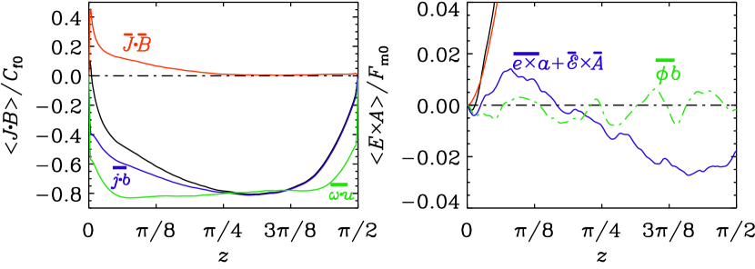
Figure 3: Magnetic helicity, current helicity, and magnetic helicity fluxes for Run A of Brandenburg (2018b) with $\mbox{\rm Re}_{\rm M}=180$. The kinetic helicity is shown in green and is found to be of similar magnitude as the current helicity of the small-scale field. The second panel shows $\overline{\bm{E}\times\bm{A}}$ near zero. The green line denotes $\overline{\phi\bm{b}}$, which is seen to fluctuate around zero.

Subsequent simulations with an outside corona indicated that the magnetic helicity changes sign at or near the outer surface (Brandenburg et al, 2009). This was just a speculation and needs to be reconsidered with the help of global models of the type considered by Warnecke et al (2011, 2012) and Brandenburg et al (2017a). This is shown in Fig. 4, where we present the line-of-sight averaged current helicity density, $\langle\bm{J}\cdot\bm{B}\rangle$ in the plane of the sky using a simulation of Brandenburg et al (2017a). The quantity $\langle\bm{J}\cdot\bm{B}\rangle$ is a proxy of magnetic helicity at small scales and shows clearly the reversal of sign between the dynamo interior and the exterior.

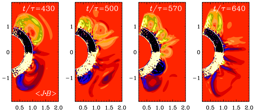
Figure 4: Current helicity $\langle\bm{J}\cdot\bm{B}\rangle$ in the plane of the observer at four different times. Yellow and white shades denote positive values and blue and black shades denote negative values; adapted from Brandenburg et al (2017a).

4.6 Radial magnetic helicity reversal in the solar wind

If the idea of alleviating catastrophic quenching by magnetic helicity fluxes is to make sense, we would expect to see signs of the expelled magnetic helicity in the solar wind. The magnetic helicity spectrum can be measured in the solar wind by determining the parity-odd contribution to the magnetic correlation tensor, which, in Fourier space, takes the form

$$\langle\tilde{B}_{i}(\bm{k})\tilde{B}^{*}_{j}(\bm{k})\rangle=\left(\delta_{ij}-\hat{k}_{i}\hat{k}_{j}\right)\,2E(k)-{\rm i}\hat{k}_{k}\epsilon_{ijk}H(k).$$ (24)

This would allow one to compute $H(k_{z})=\mbox{\rm Im}(\tilde{B}_{x}\tilde{B}_{y}^{*})$ and $E(k_{z})=\textstyle{\frac{1}{2}}(|\tilde{B}_{x}|^{2}+|\tilde{B}_{y}|^{2})$, which also obeys the realizability condition $k_{z}|H(k_{z})|\leq 2E(k_{z})$.

The Ulysses spacecraft was the only one to cover high heliographic latitudes, where a non-vanishing sign of magnetic helicity can be expected. It turned out that $H(k)$ has, as expected from dynamo theory, different signs in the northern and southern hemispheres. It also has different signs at small and large wavenumbers. This, in itself, is also expected from an $\alpha^{2}$ dynamo, because the $\alpha$ effect produces no net magnetic helicity, but it separates magnetic helicity in wavenumber space. However, the signs are opposite to what is seen at the solar surface, where the helicity in the north is negative at small length scales. In the solar wind, however, it is positive in the north and at small scales. Of course, the meaning of small is here relative and has to be with respect to larger scales, where a sign change in $k$ has been seen. If one just assumed a linear expansion of all scales from the solar surface (radius $r=700\,{\rm Mm}$, to the location of the Earth at $1\,{\rm AU}$, we expect a corresponding expansion ratio so that a wavenumber of $1\,{\rm Mm}^{-1}$ corresponds to $1/700\,{\rm AU}^{-1}$. In particular, $20\,{\rm Mm}^{-1}$ corresponds to $2/70\,{\rm AU}^{-1}$, which is close to the wavenumber where we see a sign-change in Fig. 5. It is unexpected, however, that at the solar surface (Fig. 5b), the sign in the northern hemisphere changes from minus to plus as $k$ increases, while in the solar wind, it changes from plus to minus. This apparent mismatch may not just be a measurement error, but it may actually be a real result and would tell us that the simpleminded picture of expelling magnetic helicity of one sign all the way to infinity may not be accurate.

Figure 5: Magnetic energy and magnetic helicity spectra for southern latitudes (a) at the solar surface in active region AR 11158, and (b) in the solar wind at $\sim 1\,{\rm AU}$ distance ($1\,{\rm AU}\approx 149,600\,{\rm Mm}$). Positive (negative) signs are shown as red open (blue filled) symbols. Positive signs are the solar surface at intermediate and large $k$ correspond to positive values in the solar wind at small $k$. Note that $1\,{\rm G}=10^{-4}\,{\rm T}=10^{5}\,{\rm nT}$.

When the domain is inhomogeneous, and especially when there are boundaries, magnetic helicity fluxes are possible and Eq. (18) takes the form

$$\frac{\partial}{\partial t}\overline{\bm{a}\cdot\bm{b}}=-2\overline{\mathbfcal{E}}\cdot{\overline{\bm{B}}}-2\eta\mu_{0}\,\overline{\bm{j}\cdot\bm{b}}-{\bm{\nabla}}\cdot\overline{\mathbfcal{F}}_{\rm f}.$$ (25)

In the steady state, we have

$${\bm{\nabla}}\cdot\overline{\mathbfcal{F}}_{\rm f}=\underbrace{{-2\alpha{\overline{\bm{B}}}^{2}+2\eta_{\rm t}\mu_{0}{\overline{\bm{J}}}\cdot{\overline{\bm{B}}}}}_{-2\overline{\mathbfcal{E}}\cdot{\overline{\bm{B}}}}-2\eta\mu_{0}\,\overline{\bm{j}\cdot\bm{b}}.$$ (26)

In the dynamo interior at the northern hemisphere, $\alpha>0$, and, assuming $\alpha\bm{B}^{2}$ to dominate the EMF, we expect $-2\overline{\mathbfcal{E}}\cdot{\overline{\bm{B}}}$ to be negative. However, a negative flux divergence of a negative quantity would eventually make this quantity positive, which is what has been observed.

Whether or not this is really the right interpretation remains still an open question. It would clearly be useful to have an independent assessment of this interpretation.

4.7 Nonlocal effects of $\overline{\mathbfcal{E}}$ and catastrophic quenching

Catastrophic quenching in large-scale dynamos is a rather general property. It is a consequence of the build-up of magnetic helicity of the mean magnetic field. It has been conjectured that catastrophic quenching would be prevented if the sources of toroidal field generation are spatially separated from the sources of the poloidal field; see, e.g., Tobias and Weiss (2007). This would be the case in what is known as interface dynamos (Parker, 1993). It could also be through a nonlocal $\alpha$ effect. Such a nonlocal $\alpha$ effect is an essential ingredient of the Babcock–Leighton and flux-transport dynamo models; see, Hazra et al (2023). The studies of Brandenburg and Käpylä (2007) and Chatterjee et al (2010) showed that a spatial separation between shear and $\alpha$ effects does in general not help to avoid catastrophic quenching for such types of dynamo models. It is interesting, however, that Kitchatinov and Olemskoy (2011) and later also Brandenburg and Hubbard (2015) found that the inclusion of diamagnetic downward pumping of the toroidal magnetic field can alleviate the catastrophic quenching in the Babcock–Leighton dynamo model with a strongly nonlocal $\alpha$.

The catastrophic quenching models are reasonably well reproduced by DNS when the geometries of the setups are sufficiently simple. It would therefore be worthwhile to apply DNS to conditions where turbulent pumping and a strongly nonlocal mean electromotive force can be expected. At present, however, even just the physical reality of a nonlocal $\alpha$ effect of Babcock–Leighton type through the decay of active regions rests mainly on the interpretation of solar observations. Turbulence simulations have so far not been able to make contact with such concepts.

5 Alternative large-scale dynamo effects

Given the difficulties encountered with $\alpha$ effect dynamos, there have been various attempts to construct large-scale dynamos that are not based on the $\alpha$ effect. A common misconception here is the idea that catastrophic quenching would not apply if just because there is no $\alpha$ effect. This is not true, because an $\alpha_{\rm M}$ term can always emerge regardless of whether or not there existed an original $\alpha$ effect. An example is the shear–current effect. It is due to the presence of shear and boundaries that a helicity can be introduced. Shear of the form $\overline{\bm{U}}=(0,Sx,0)$ implies a finite vorticity, ${\bm{\nabla}}\times\overline{\bm{U}}=(0,0,S)$ and boundaries would lead to a gradient vector of turbulent intensity near the boundaries. Thus, while there can be hope that catastrophic quenching may not be as strong, this may turn out not to be the case. An example of this was presented in Brandenburg and Subramanian (2005c).

5.1 Rädler and shear–current effects

The Rädler effect is another large-scale dynamo effect (Rädler, 1969). In the simplest representation it leads to an EMF proportional to $\bm{\Omega}\times{\overline{\bm{J}}}$. It is similar to the shear–current effect. In this case it cannot change the magnetic energy of the mean field. Indeed, the energy equation for the mean field is given by

$$\frac{{\rm d}{}}{{\rm d}{}t}\langle{\overline{\bm{B}}}^{2}/2\rangle=\underbrace{{\overline{\bm{J}}}\cdot(\bm{\Omega}\times{\overline{\bm{J}}})}_{=0}+\underbrace{\langle{\bm{\nabla}}\cdot[(\bm{\Omega}\times{\overline{\bm{J}}})\times{\overline{\bm{B}}}]\rangle}_{\mbox{$=0$ under periodicity}}.$$ (27)

In the general case, the generation effects due to global rotation and mean currents can be written as follows (see Krause and Rädler, 1980; Kitchatinov et al, 1994; Rädler et al, 2003; Pipin, 2008):

$$\overline{\mathbfcal{E}}^{(\delta)}=\delta_{1}\bm{\Omega}\times{\overline{\bm{J}}}+\delta_{2}\bm{\nabla}\left(\bm{\Omega}\cdot{\overline{\bm{B}}}\right)+\delta_{3}\frac{\bm{\Omega}\left[\bm{\Omega}\cdot\bm{\nabla}\left(\bm{\Omega}\cdot{\overline{\bm{B}}}\right)\right]}{\bm{\Omega}^{2}},$$ (28)

where the coefficients $\delta_{1,2,3}$ depend on the spatial profiles of the turbulent parameters such as the typical convective turnover time, the convective velocity $u_{\rm rms}$, etc. The last two terms in this equation may lead to an $\delta^{2}$ dynamo (Pipin and Seehafer, 2009). For the solar case, the $\delta$ effect can provide an additional non-helical source of poloidal magnetic field generation. Interestingly, Pipin and Seehafer (2009) found that for the solar-type dynamos, i.e., those with equatorward propagation of the dynamo waves, the $\delta$ dynamo effect does not dominate the contributions of the $\alpha$-effect. We will discuss the available scenario in the next section.

5.2 Dynamos from negative turbulent magnetic diffusivity

There are two other effects that are noteworthy, although it is not clear that either of them can play a role in stellar convection zones. One is the negative turbulent magnetic diffusivity and the other is the memory effect in conjunction with a pumping effect.

When modeling a negative turbulent magnetic diffusivity dynamo, high wavenumbers must not be destabilized at the same time. Brandenburg and Chen (2020) studied classes of dynamos with a very low critical $\mbox{\rm Re}_{\rm M}$. The Willis dynamo (Willis, 2012) has a critical $\mbox{\rm Re}_{\rm M}$ of 2.01, which is small compared to 6.3 for the Roberts flow and 17.9 for the ABC flow. In this dynamo, one of the two horizontally averaged field components grows exponentially, because the total magnetic diffusivity in that direction is negative (Brandenburg and Chen, 2020). The other component decays and is not coupled to the former one.

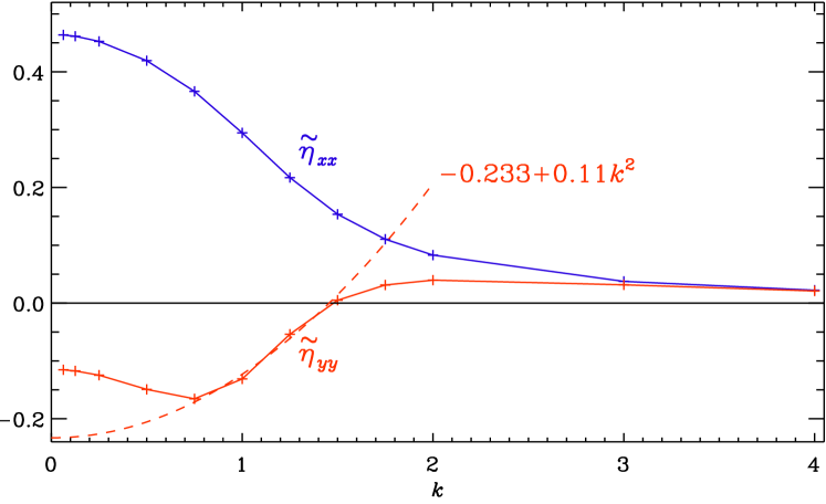
Figure 6: Dependence of $\tilde{\eta}_{xx}$ (blue) and $\tilde{\eta}_{yy}$ (red) on $k$ for the Willis flow in the marginally exited case with $\eta=0.403$. The red dashed line denotes the fit $-0.233+0.11\,k^{2}$. Adapted from Brandenburg and Chen (2020).

As we see from Fig. 6, $\eta_{\rm t}$ is negative only for $k\mathrel{\mathchoice{\vbox{\offinterlineskip\halign{\hfil$\displaystyle#$\hfil\cr<\cr\sim\cr}}}{\vbox{\offinterlineskip\halign{\hfil$\textstyle#$\hfil\cr<\cr\sim\cr}}}{\vbox{\offinterlineskip\halign{\hfil$\scriptstyle#$\hfil\cr<\cr\sim\cr}}}{\vbox{\offinterlineskip\halign{\hfil$\scriptscriptstyle#$\hfil\cr<\cr\sim\cr}}}}1.5$. The $k$ dependence of the turbulent magnetic diffusivity can be expanded up to second order as

$$\tilde{\eta}_{yy}(k)=\tilde{\eta}_{yy}^{(0)}+\tilde{\eta}_{yy}^{(2)}k^{2}+\ldots,$$ (29)

where the tildes indicate Fourier transformed quantities. In the proximity of $k=1$, which corresponds to the largest scale in the computational domain of $2\pi$, we have $\tilde{\eta}_{yy}^{(0)}\approx-0.233$ and $\tilde{\eta}_{yy}^{(2)}\approx 0.11$. In addition, there is still the microphysical magnetic diffusivity, which is positive ($\eta=0.403$). To a first approximation, one can just consider the equation for $\overline{A}_{yy}$, which can then be written as

$${\partial\overline{A}_{yy}\over\partial t}=\left[\eta+\tilde{\eta}_{yy}^{(0)}\right]{\partial^{2}\overline{A}_{yy}\over\partial z^{2}}-\tilde{\eta}_{yy}^{(2)}{\partial^{4}\overline{A}_{yy}\over\partial z^{4}}.$$ (30)

We recall that the minus sign in front of the fourth derivative corresponds to positive diffusion if $\tilde{\eta}_{yy}^{(2)}$ is positive, and so does the plus sign in front of the second derivative, unless the term in squared brackets is negative, which is the case we are considering here.

5.3 Dynamos from pumping and memory effects

Pumping effects alone cannot usually lead to interesting dynamo effects, unless there is also a memory effect. This effect means that the mean electromotive force depends not just on the instantaneous mean magnetic field at that time, but also on the mean magnetic field at earlier times. It is therefore described as a convolution between a pumping kernel and the mean magnetic field. This can lead to dynamo action, as has been demonstrated by Rheinhardt et al (2014) for the case of two of the four flow fields studied by Roberts (1972). These are flows II and III with $\bm{U}_{\rm II}(x,y)$ and $\bm{U}_{\rm III}(x,y)$, respectively, and are given by

$$\bm{U}_{\rm II}=\begin{pmatrix}u_{0}\sin Kx\cos Ky\\ -u_{0}\cos Kx\sin Ky\\ u_{0}\cos Kx\cos Ky\end{pmatrix},\quad\bm{U}_{\rm III}=\begin{pmatrix}u_{0}\sin Kx\cos Ky\\ -u_{0}\cos Kx\sin Ky\\ \textstyle{\frac{1}{2}}u_{0}(\cos 2Kx+\cos 2Ky)\end{pmatrix},$$ (31)

where $K$ is the wavenumber of the flow. Both flows have zero kinetic helicity and no $\alpha$ effect, but flow II is also pointwise nonhelical. A supercritical three-dimensional magnetic field with growth rate $\gamma$ and wavenumber $k$ in the $z$ direction of the form $\bm{B}=\bm{b}_{0}(x,y)\,e^{\gamma t+{\rm i}kz}$ is possible when $\mbox{\rm Re}_{\rm M}\equiv u_{0}/\eta K>4.58$ and 2.9 for flows II and III, respectively; see Rheinhardt et al (2014). Here, $\bm{b}_{0}(x,y)$ is the eigenfunction.

For both flows, there are $xy$-averaged mean fields $\overline{B}_{x}(z,t)$ and $\overline{B}_{y}(z,t)$, with waves traveling in opposite directions for flow II and in the same direction for flow III; see Figures 6 and 8 of Rheinhardt et al (2014), respectively. These dynamos appear to be atypical, because there is so far no other known example of a flow where pumping produces a memory effect that is strong enough to lead to dynamo action. This may well be due to the absence (until recently) of computational tools for determining the memory effect. Indeed, it was only with the development of the TFM (Schrinner et al, 2005, 2007) that the importance of the memory effect was noticed (Hubbard and Brandenburg, 2009) and applied to pumping.

The dispersion relation for a problem with turbulent pumping $\gamma$ and turbulent magnetic diffusion $\eta_{\rm t}$ is given by $\lambda=-{\rm i}k\gamma-\eta_{\rm t}k^{2}$. Since $\mbox{\rm Re}\lambda<0$, the solution can only decay, but it is oscillating with the frequency $\omega=\mbox{\rm Im}\lambda=\gamma$. In the presence of a memory effect, $\gamma$ is replaced by $\gamma/(1-{\rm i}\omega\tau)$, where $\tau$ is the memory time. Then, $\lambda\approx-{\rm i}k\gamma\,(1-{\rm i}\omega\tau)-\eta_{\rm t}k^{2}$, and $\mbox{\rm Re}\lambda$ can be positive. This is the case for the Roberts flows II and III.

We return to nonlocality and memory effects further below in this article when we discuss concrete solar models; see Pipin (2023). One of the most obvious consequences of the memory effect is a lowering of the critical excitation conditions for the dynamo, which was already reported by Rheinhardt and Brandenburg (2012). Interestingly, for the nonlocal mean electromotive force, the lowering of the critical threshold can be accompanied by multiple instabilities of different dynamo modes that have different frequencies and spatial localization; see Pipin (2023).

5.4 Dynamos from cross-helicity

An alignment of velocity and magnetic field, i.e., cross helicity, plays a key role in numerous processes and phenomena of astrophysical plasmas. Krause and Rädler (1980) showed that the saturation stage of the turbulent generation is characterized by an alignment of the turbulent convective velocity and the magnetic field. This consideration does not account for the effects of cross-helicity that take place in the strongly stratified subsurface layers of the stellar convective envelope. For example, the direct numerical simulations of Matthaeus et al (2008) showed a directional alignment of velocity and magnetic field fluctuations in the presence of gradients of either pressure or kinetic energy.

The mean electromotive force in this case is along to the mean vorticity,

$$\overline{\mathbfcal{E}}^{\Upsilon}=\Upsilon\nabla\times\overline{\mathbf{U}}+\dots,$$ (32)

where, $\Upsilon=\tau_{c}\left\langle\mathbf{u}^{(0)}\cdot\mathbf{b}^{(0)}\right\rangle$ is the cross helicity pseudoscalar, and $\tau_{c}$ is the turbulent turnover time. The superscripts ${(0)}$ indicate quantities of the background turbulence, which exists in the absence of a mean magnetic field and a mean flow; see our comment after Eq. (2) about the $\overline{\mathbfcal{E}}_{0}$ term. In the standard mean-field framework, it is assumed that $\Upsilon=0$; see Krause and Rädler (1980). Yoshizawa and Yokoi (1993) generalized the framework assuming $\Upsilon\neq 0$, see the comprehensive review of Yokoi (2013).

Dynamo scenarios based on cross helicity have been suggested in a number of papers (Yoshizawa and Yokoi, 1993; Yoshizawa et al, 2000; Yokoi, 2013). Pipin and Yokoi (2018) showed that the large-scale dynamo instability does not require the existence of a global axisymmetric mean. The mix of axisymmetric and nonaxisymmetric magnetic fields can be produced even in the case $\overline{\Upsilon=0}$, where the overbar means azimuthal averaging. The surface magnetic field of the Sun and other similar stars tends to be organized in sunspots, plagues, ephemeral regions, super-granular magnetic network, etc. These structures tend to demonstrate the alignment of local velocity and magnetic fields (Rüdiger et al, 2011). Therefore, the cross helicity dynamo instability can contribute to dynamo generation effects that operate near the stellar surface. Stellar observations, for example those of Katsova et al (2021), require such dynamo effects to be working in situ at the stellar surface. The solar analogs show an increase of the spottiness with an increase of the rotation rate (Berdyugina, 2005). In that case, cross helicity dynamo effects can be considered as a relevant addition to the standard turbulent generation by means of convective helical motions. Rapidly rotating M-dwarfs show the highest level of magnetic activity (Kochukhov, 2021). There is a population of rapidly rotating M-dwarfs that show a rather strong dipole type magnetic field. These stars show a rather small level of differential rotation. For solid body rotation, an $\alpha^{2}$ dynamo generates a nonaxisymmetric magnetic field (Chabrier and Küker, 2006; Elstner and Rüdiger, 2007). At high rotation rates, the $\alpha$ effect is highly anisotropic (Rüdiger and Kitchatinov, 1993). It cannot employ the component of the large-scale magnetic field along the rotation axis for the generation of an axial electromotive force. Results of Pipin and Yokoi (2018) show that the $\alpha^{2}\Upsilon^{2}$ scenario can produce a strong constant dipole magnetic field. The model predicts the existence of large-scale cross helicity patterns occupying the stellar surface. We hope that this can be tested either in observations or in GCDs.

The nonlinear theory for the cross helicity effect is not yet developed. Sur and Brandenburg (2009) showed that the turbulent generation due to $\Upsilon$ is quenched by large-scale vorticity in a way that is similar to catastrophic quenching given by Eq. (20), i.e.,

$$\Upsilon\sim\frac{1}{1+\mbox{\rm Re}_{\rm M}\tau_{c}^{2}({\bm{\nabla}}\times\overline{\mathbf{U}})^{2}}.$$ (33)

One should remember that for the initialization of the cross-helicity dynamo instability we have to seed both the cross helicity and the magnetic field. The solar type model scenarios based on cross helicity require an $\alpha$ effect, which produces poloidal magnetic field and cross helicity at the top of the dynamo domain (Yokoi et al, 2016).

Given that cross helicity is an ideal invariant of the MHD equations, it is natural to ask whether systems with strong cross helicity exhibit inverse cascading. The answer seems to be yes; see Brandenburg et al (2014). In Fig. 7 we demonstrate the gradual build-up of magnetic fields in the vertical direction when the system has significant cross helicity owing to the presence of a magnetic field along the direction of gravity (Rüdiger et al, 2011).

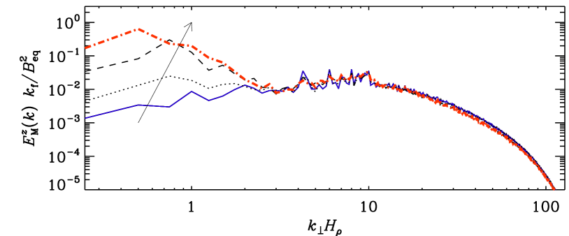
Figure 7: Normalized spectra of $B_{z}$ from a simulation of MHD turbulence with strong gravity at turbulent diffusive times $t\eta_{\rm t}/H_{\rho}^{2}\approx 0.2$, 0.5, 1, and 2.7 with $k_{\rm f}H_{\rho}=10$ and $k_{1}H_{\rho}=0.25$. Adapted from Brandenburg et al (2014).

6 Mean-field dynamo models

In general, the $\alpha$ effect, as well as any other turbulent generation effect, including the $\delta$ effect (Rädler, 1969), the shear-current effect (Kleeorin et al, 2000), and the cross-helicity effect (Yokoi, 2013) can generate both toroidal and poloidal magnetic fields. Therefore there can be a number of possibilities for solar-types dynamo models Krause and Rädler (1980); Yokoi et al (2016); Pipin and Kosovichev (2018). Some of them skip the $\alpha$ effect altogether. For example, Seehafer and Pipin (2009) studied $\delta^{\Omega}\Omega$ and $\delta^{W}\Omega$ scenarios, where turbulent generation of the poloidal magnetic field is due to $\bm{\Omega}\times{\overline{\bm{J}}}$ and shear-current effect, respectively. These scenarios show oscillating solutions and the correct time-latitude diagram of the toroidal magnetic field if the meridional circulation is included. A similar possibility was mentioned earlier by Krause and Rädler (1980) for the $\delta\Omega$ scenario. However, the given scenarios result in an incorrect phase relation between activity of the toroidal and poloidal magnetic fields. The aim to search for $\alpha$ effect alternatives pursues double benefits. First, the nonhelical source of dynamo generations avoids the above mentioned catastrophic quenching problem. This issue is less important currently. Secondly, and it was already mentioned earlier by Köhler (1973) as well as Steenbeck and Krause (1969), the mixing length estimate of the $\alpha$ effect for the solar convection zone parameters results in a very strong $\alpha$ effect with a magnitude as strong as the convective velocity rms. Solar observations of the ratio between the typical strength of the toroidal and poloidal fields and the solar cycle period, favor an order of magnitude smaller $\alpha$ effect. In addition, the turbulent generation sources in the $\alpha\Omega$ scenario help reduce the given constraints. We must stress that the GCD simulations of Schrinner (2011), Schrinner et al (2011), and Warnecke et al (2021) showed that the mean-field models need a full spectrum of turbulent effects to describe DNS.

In the case of a solar-like star, i.e., with solar-like stratification, differential rotation, and meridional circulation profiles, the turbulent sources of the poloidal magnetic field generation due to $\delta$, shear-current, and cross-helicity effects are likely complimentary to the $\alpha$ effect.

We thus arrive at the conclusion that the $\alpha^{2}\Omega$ dynamo is, probably, the simplest scenario for the solar dynamo. Also, this scenario seems to fit well with observations of stellar activity of young solar-type stars.

6.1 Basic model

We discuss some results of the state-of-the-art mean-field dynamo model of a solar dynamo developed recently by Pipin and Kosovichev (2019) (hereafter PK19). The magnetic field evolution is governed by the mean-field induction equation:

$$\frac{\partial{\overline{\bm{B}}}}{\partial t}=\mathbf{\nabla}\times\left(\overline{\mathbfcal{E}}+\overline{\bm{U}}\times{\overline{\bm{B}}}-\eta\mu_{0}{\overline{\bm{J}}}\right).$$ (34)

The expression for the components of $\overline{\mathbfcal{E}}$ reads

$$\overline{\mathcal{E}}_{i}=\left(\alpha_{ij}+\gamma_{ij}\right)\overline{B}{}_{j}-\eta_{ijk}\nabla_{j}\overline{B}{}_{k}.$$ (35)

Here, $\alpha_{ij}$ describes the turbulent generation by the $\alpha$ effect, $\gamma_{ij}$ represents turbulent pumping, and $\eta_{ijk}$ is the eddy magnetic diffusivity tensor. The $\alpha$ effect tensor includes the small-scale magnetic helicity density contribution, i.e., the pseudoscalar $\left\langle\mathbf{a}\cdot\mathbf{b}\right\rangle$,

$$\alpha_{ij} = C_{\alpha}\psi_{\alpha}(\beta)\alpha_{ij}^{\rm K}+\alpha_{ij}^{\rm M}\psi_{\alpha}(\beta)\frac{\left\langle\mathbf{a}\cdot\mathbf{b}\right\rangle\tau_{c}}{4\pi\overline{\rho}\ell_{c}^{2}},$$ (36)

where $C_{\alpha}$ is the dynamo parameter characterizing the magnitude of the kinetic $\alpha$ effect, and $\alpha_{ij}^{\rm K}$ and $\alpha_{ij}^{\rm M}$ are the anisotropic versions of the kinetic and magnetic $\alpha$ effects, as described in PK19. Note that, unlike Eq. (16), where the two $\alpha$ contributions are pseudoscalars and have the same dimension, they are here tensorial where only $\alpha_{ij}^{\rm K}$ is a pseudotensor, but $\alpha_{ij}^{\rm M}$ is not, and they have here different dimensions.

The radial profiles of $\alpha_{ij}^{(H)}$ and $\alpha_{ij}^{(M)}$ depend on the mean density stratification, the profile of the convective velocity $u_{\rm rms}$, and on the Coriolis number,

$${\rm Co}=2\Omega_{0}\tau_{c},$$ (37)

where $\Omega_{0}$ is the global angular velocity of the star and $\tau_{c}$ is the convective turnover time. The magnetic quenching function $\psi_{\alpha}(\beta)$ depends on the parameter $\beta=|{\overline{\bm{B}}}|/(\sqrt{4\pi\overline{\rho}}u_{\rm rms})$. In this model the magnetic helicity is governed by the global conservation law for the total magnetic helicity, $\left\langle\mathbf{A}\cdot\mathbf{B}\right\rangle=\left\langle\mathbf{a}\cdot\mathbf{b}\right\rangle+{\overline{\bm{A}}}\cdot{\overline{\bm{B}}}$ (see Hubbard and Brandenburg, 2012; Pipin et al, 2013):

$$\left(\frac{\partial}{\partial t}+\overline{\bm{U}}\cdot\bm{\nabla}\right)\left\langle\mathbf{A}\cdot\mathbf{B}\right\rangle=-\frac{\left\langle\mathbf{a}\cdot\mathbf{b}\right\rangle}{\mbox{\rm Re}_{\rm M}\tau_{c}}-2\eta{\overline{\bm{B}}}\cdot{\overline{\bm{J}}}-\mathbf{\nabla\cdot}\overline{\mathbfcal{F}}_{\rm f},$$ (38)

where we have used $2\eta\mathbf{\left\langle j\cdot b\right\rangle}=\left\langle\mathbf{a}\cdot\mathbf{b}\right\rangle/{\mbox{\rm Re}_{\rm M}\tau_{c}}$ (Kleeorin and Rogachevskii, 1999). Also, we have introduced a diffusive flux of the small-scale magnetic helicity density, $\overline{\mathbfcal{F}}_{\rm f}=-\eta_{\chi}\mathbf{\nabla}\left\langle\mathbf{a}\cdot\mathbf{b}\right\rangle$, and $\mbox{\rm Re}_{\rm M}$ is the magnetic Reynolds number, for which we employ $\mbox{\rm Re}_{\rm M}=10^{6}$. Following results of Mitra et al (2010a), we put $\eta_{\chi}=0.1\,\eta_{T}$. Here, the turbulent fluxes of the magnetic helicity are approximated by the only term which is related to the diffusive flux. Besides the diffusive helicity flux, the other turbulent fluxes of the magnetic helicity can be important for the nonlinear dynamo regimes and the catastrophic quenching problem (Kleeorin et al, 2000; Vishniac and Cho, 2001; Pipin, 2008; Chatterjee et al, 2011; Brandenburg and Subramanian, 2005a; Kleeorin and Rogachevskii, 2022; Gopalakrishnan and Subramanian, 2023). The relative importance of different kinds of magnetic helicity fluxes for the dynamo should be studied further.

The above ansatz for the helicity evolution differs from that given by Eq. (18); see also papers by Kleeorin and Ruzmaikin (1982) and Kleeorin and Rogachevskii (1999). Hubbard and Brandenburg (2012) had studied the magnetic helicity evolution for shearing dynamos. They found that employing Eq. (18) in the dynamo problem can result in nonphysical fluxes of magnetic helicity over spatial scales. For the ansatz given by Eq. (18), the nonlinear dynamo models can show sharp magnetic structures inside the dynamo domain. Such structures are connected with concentrations of the magnetic helicity; see, e.g., Chatterjee et al (2011) and Brandenburg and Chatterjee (2018). Even a strong diffusive helicity flux does not seem to correct for those irrelevant features from the numerical solution. The technical point is that the helicity fluxes, which are omitted in Eq. (18), should be consistent with the turbulent effects involved in the mean electromotive force, e.g., the rotationally induced anisotropy of the $\alpha$ effect, the magnetic eddy diffusivity, etc. Such calculations are currently absent. Also, we have to take into account the modulation of the magnetic helicity density by the magnetic activity. On the other hand, with the magnetic helicity evolution equation Eq. (38), Pipin et al (2013) found that magnetic helicity density follows the large-scale dynamo wave. This alleviates the catastrophic quenching of the $\alpha$ effect. They showed that if we write the Eq. (38) in the form of Eq. (18), we get an additional helicity flux due to the global dynamo, Rewriting Eq. (38) in the form of Eq. (18) we get

$$\frac{\partial\left\langle\mathbf{a}\cdot\mathbf{b}\right\rangle}{\partial t}=-2\left(\overline{\mathbfcal{E}}\cdot\overline{\bm{B}}\right)-\frac{\left\langle\mathbf{a}\cdot\mathbf{b}\right\rangle}{\mbox{\rm Re}_{\rm M}\tau_{c}}+\bm{\nabla}\cdot\left(\eta_{\chi}\bm{\nabla}\left\langle\mathbf{a}\cdot\mathbf{b}\right\rangle\right)-\eta\overline{\mathbf{B}}\cdot\mathbf{\overline{J}}-\bm{\nabla}\cdot\left(\overline{\mathbfcal{E}}\times{\overline{\bm{A}}}\right)+\dots,$$ (39)

where the ellipsis refers to additional helicity transport terms due to the large-scale flow. The term $\overline{\mathbfcal{E}}\times\overline{\mathbf{A}}$ consists of the counterparts of the sources of magnetic helicity, which are represented by $-2\overline{\mathbfcal{E}}\cdot\overline{\mathbf{B}}$, and the fluxes which result from pumping of the large-scale magnetic fields. The sources of magnetic helicity in the term $-2\overline{\mathbfcal{E}}\cdot\overline{\bm{B}}$ are partly compensated in Eq. (39) by the counterparts in $\overline{\mathbfcal{E}}\times{\overline{\bm{A}}}$. This results in the spatially homogeneous quenching of the large-scale magnetic generation and alleviation of the catastrophic quenching problem. The effect of $\overline{\mathbfcal{E}}\times{\overline{\bm{A}}}$ was not unambiguously confirmed in DNS because of limited numerical resolution; see Del Sordo et al (2013) and Brandenburg (2018b).

The turbulent pumping is expressed by the antisymmetric tensor $\gamma_{ij}$. The tuning of $\gamma_{ij}$ for the solar-type mean-field dynamo model was discussed by Pipin (2018). We define it as follows,

$$\gamma_{ij} = \gamma_{ij}^{(\Lambda\rho)}+\frac{\alpha_{\mathrm{MLT}}u_{\rm rms}}{\gamma}\mathcal{H}\left(\beta\right)\mathrm{\hat{r}_{n}\varepsilon_{inj}},$$ (40)

$$\gamma_{ij}^{(\Lambda\rho)} = 3\nu_{T}f_{1}^{(a)}\left\{\left(\mathbf{\bm{\Omega}}\cdot\bm{\Lambda}^{(\rho)}\right)\frac{\Omega_{n}}{\Omega^{2}}\varepsilon_{\mathrm{inj}}-\frac{\Omega_{j}}{\Omega^{2}}\mathrm{\varepsilon_{inm}\Omega_{n}\Lambda_{m}^{(\rho)}}\right\},$$ (41)

where $\mathbf{\bm{\Lambda}}^{(\rho)}=\bm{\nabla}\log\overline{\rho}$ , $\mathrm{\alpha_{MLT}}=1.9$ is the mixing-length theory parameter, $\gamma$ is the adiabatic law constant. In Eq. (40), the first term takes into account the mean drift of large-scale field due the gradient of the mean density, and the second one does the same for the mean-field magnetic buoyancy effect. The function $\mathcal{H}\left(\beta\right)$ takes into account the effect of the magnetic tensions. It is $\mathcal{H}\left(\beta\right)\sim\beta^{2}$ for small $\beta$ and it saturates as $\beta^{-2}$ for $\beta\gg 1$; see P22.

We employ an anisotropic diffusion tensor following the formulation of Pipin (2008) (hereafter, P08):

$$\eta_{ijk} = 3\eta_{T}\left\{\left(2f_{1}^{(a)}-f_{2}^{(d)}\right)\varepsilon_{ijk}+2f_{1}^{(a)}\frac{\Omega_{i}\Omega_{n}}{\Omega^{2}}\varepsilon_{jnk}\right\},$$ (42)

where the functions $f_{1,2}^{(a,d)}\left(\Omega^{*}\right)$ are determined in P08. Analytical calculations of $\overline{\mathbfcal{E}}$ in the above cited paper include the effects of a small scale dynamo. In the above expressions for $\overline{\mathbfcal{E}}$, we assume equipartition between kinetic energy of the turbulence and magnetic fluctuations which stem from the small-scale dynamo. It was found that for the case of slow rotation (${\rm Co}\ll 1$), the part of $\overline{\mathbfcal{E}}$ that depends on the gradients of ${\overline{\bm{B}}}$ consists of an isotropic eddy diffusivity and Rädler’s $\bm{\Omega}\times{\overline{\bm{J}}}$ effect due to the small-scale dynamo (see also Rädler et al, 2003). In the case of rapid rotation, the fluctuating magnetic fields from the small-scale dynamo contribute both to isotropic and anisotropic parts of the diffusivity. The effect appears already in the terms of order $\Omega^{2}$ in the global rotation rate (Rädler et al, 2003). In particular, the part of EMF which corresponds to Eq(42 can be written as

$$\overline{\mathbfcal{E}}^{\eta} = -3\eta_{T}\left(2f_{1}^{(a)}-f_{2}^{(d)}\right){\overline{\bm{J}}}+6\eta_{T}f_{1}^{(a)}\bm{\Omega}\frac{\bm{\Omega}\cdot{\overline{\bm{J}}}}{\Omega^{2}}.$$ (43)

It is noteworthy that the full expression for $\overline{\mathbfcal{E}}$ obtained in P08 is complicated and includes other contributions due to the effects of global rotation $\bm{\Omega}$, mean shear, mean current density ${\overline{\bm{J}}}$, and the magnetic deformation tensor $(\nabla{\overline{\bm{B}}})$. We skip them in the application to the solar dynamo model. The analytical results about the relations of the specific effects of $\overline{\mathbfcal{E}}$ and the global rotation rate show qualitative agreement with the DNS of Käpylä et al (2009a) and Brandenburg et al (2012). Yet, a more detailed comparison of the analytical results and the GCD simulations is needed; for further discussions, see Sect. 7.

We assume that the large-scale flow is axisymmetric. It is decomposed into the sum of meridional circulation and differential rotation, $\mathbf{\overline{U}}=\mathbf{\overline{U}}^{m}+r\sin\theta\Omega\left(r,\theta\right)\hat{\mathbf{\bm{\phi}}}$, where $r$ is the radial coordinate, $\theta$ is the polar angle, $\hat{\mathbf{\bm{\phi}}}$ is is the unit vector in the azimuthal direction, and $\Omega\left(r,\theta\right)$ is the angular velocity profile. The angular momentum conservation and the equation for the azimuthal component of large-scale vorticity, $\mathrm{\overline{\omega}=(\bm{\nabla}\times\overline{\mathbf{U}}^{m})_{\phi}}$, determine the distributions of differential rotation and meridional circulation:

$$\frac{\partial}{\partial t}\overline{\rho}r^{2}\sin^{2}\theta\Omega=-\bm{\nabla\cdot}\left[r\sin\theta\overline{\rho}\left(\hat{\mathbf{T}}_{\phi}+r\sin\theta\Omega\mathbf{\overline{U}^{m}}\right)\right]+\bm{\nabla\cdot}\left[r\sin\theta\frac{{\overline{\bm{B}}}\overline{B}_{\phi}}{4\pi}\right],$$ (44)

$$\frac{\partial\omega}{\partial t} = r\sin\theta\bm{\nabla}\cdot\left[\frac{\hat{\bm{\phi}}\times\bm{\nabla\cdot}\overline{\rho}\hat{\mathbf{T}}}{r\overline{\rho}\sin\theta}-\frac{\mathbf{\overline{U}}^{m}\overline{\omega}}{r\sin\theta}\right]+r\sin\theta\frac{\partial\Omega^{2}}{\partial z}-\frac{g}{c_{p}r}\frac{\partial\overline{s}}{\partial\theta}$$

$$+ \frac{1}{4\pi\overline{\rho}}\left({\overline{\bm{B}}}\bm{\cdot\nabla}\right)\left(\bm{\nabla}\times{\overline{\bm{B}}}\right)_{\phi}-\frac{1}{4\pi\overline{\rho}}\left[\left(\bm{\nabla}\times{\overline{\bm{B}}}\right)\bm{\cdot\nabla}\right]\overline{B}{}_{\phi},$$

where $\hat{\mathbf{T}}$ is the turbulent stress tensor:

$$\hat{T}_{ij}=\left\langle u_{i}u_{j}\right\rangle-\frac{1}{4\pi\overline{\rho}}\left(\left\langle b_{i}b_{j}\right\rangle-\frac{1}{2}\delta_{ij}\left\langle\mathbf{b}^{2}\right\rangle\right);$$ (45)

see the detailed description in Pipin and Kosovichev (2018) and PK19. Also, $\overline{\rho}$ is the mean density, $\overline{s}$ is the mean entropy; $\partial/\partial z=\cos\theta\partial/\partial r-\sin\theta/r\cdot\partial/\partial\theta$ is the gradient along the axis of rotation. The mean heat transport equation determines the mean entropy variations from the reference state due to the generation and dissipation of the large-scale magnetic field and large-scale flows:

$$\overline{\rho}\overline{T}\left[\frac{\partial\overline{\mathrm{s}}}{\partial t}+\left(\overline{\mathbf{U}}\cdot\bm{\nabla}\right)\overline{\mathrm{s}}\right]=-\bm{\nabla}\cdot\left(\mathbf{F}^{c}+\mathbf{F}^{r}\right)-\hat{T}_{ij}\frac{\partial\overline{U}_{i}}{\partial r_{j}}-\overline{\mathbfcal{E}}\cdot{\overline{\bm{J}}},$$ (46)

where $\overline{T}$ is the mean temperature, $\mathbf{F}^{r}$ is the radiative heat flux, $\mathbf{F}^{c}$ is the anisotropic convective flux; see PK19. The last two terms in Eq. (46) take into account the convective energy gain and loss caused by the generation and dissipation of large-scale magnetic fields and large-scale flows. The reference profiles of mean thermodynamic parameters, such as entropy, density, and temperature are determined from the stellar interior model MESA (Paxton et al, 2015). The radial profile of the typical convective turnover time, $\tau_{c}$, is determined from the MESA code, as well. We assume that $\tau_{c}$ does not depend on the magnetic field and global flows. The convective rms velocity is determined from the mixing-length approximation,

$$u_{\rm c}=\frac{\ell_{c}}{2}\sqrt{-\frac{g}{2c_{p}}\frac{\partial\overline{s}}{\partial r}},$$ (47)

where $\ell_{c}=\alpha_{\mathrm{MLT}}H_{p}$ is the mixing length, $\alpha_{\mathrm{MLT}}=1.9$ is the mixing length parameter, and $H_{p}$ is the pressure height scale. Equation (47) determines the reference profiles for the eddy heat conductivity $\chi_{T}$, eddy viscosity $\nu_{T}$, and eddy magnetic diffusivity $\eta_{T}$,

$$\chi_{T} = \frac{\ell^{2}}{6}\sqrt{-\frac{g}{2c_{p}}\frac{\partial\overline{s}}{\partial r}},$$ (48)

$$\nu_{T} = \mathrm{Pr_{\rm T}}\,\chi_{\rm T},$$ (49)

$$\eta_{T} = \mathrm{Pm_{\rm T}}\,\nu_{\rm T}.$$ (50)

It should be noted that stellar convection might well have convection zones with slightly subadiabatic stratification in some layers. In those cases, the enthalpy flux can no longer be transported entirely by the mean entropy gradient, but there can be an extra term that is nowadays called the Deardorff term; see Deardorff (1972). Such convection can be driven through the rapid cooling in the surface layers and is therefore sometimes referred to as entropy rain Brandenburg (2016). It is useful to stress that the Deardorff term is distinct from the usual overshoot, because there the enthalpy flux points downward, while entropy rain still produces an outward enthalpy flux. It is instead more similar to semiconvection.

Boundary conditions. At the bottom of the tachocline, $r_{\rm i}=0.68\,R$, we assume solid body rotation and perfect conductor boundary conditions. Following to the MESA solar interior model, we put the bottom of the convection zone to $r_{\rm b}=0.728\,R$. At this boundary we fix the total heat flux, $F_{\rm r}^{\rm conv}+F_{\rm r}^{\rm rad}=L_{\star}(r_{b})/4\pi r_{b}^{2}$. We introduce the decrease by $\exp\left(-100\,z/R\right)$ for all turbulent coefficients (except the eddy viscosity and eddy diffusivity), where $z$ is the distance from the bottom of the convection zone. The decrease of the eddy viscosity and eddy diffusivity is at most one order of magnitude for numerical stability. The meridional circulation is restricted to the convection zone. Therefore, we put the azimuthal component of the large-scale vorticity to zero, i.e., we set $\mathrm{\overline{\omega}}=0$ at $r_{\rm b}$. At the top, $r_{\rm t}=0.99\,R$, we employ a stress free and black body radiating boundary. Following ideas of Moss and Brandenburg (1992), we formulate the top boundary condition in a form that allows penetration of the toroidal magnetic field to the surface:

$$\delta\frac{\eta_{T}}{r_{\mathrm{top}}}B\left[1+\left(\frac{\left|B\right|}{B_{\mathrm{esq}}}\right)\right]+\left(1-\delta\right)\mathcal{E}_{\theta} = 0,$$ (51)

Free parameters. The model employs a number of free parameters, including $C_{\alpha}$, the turbulent Prandtl numbers $\mbox{\rm Pr}_{\rm T}$ and $\mbox{\rm Pr}_{\rm M,T}$, $\delta$, $B_{\mathrm{esq}}$, and the global rotation rate $\Omega_{0}$. For the solar case we use a period of rotation of the solar tachocline determined from helioseismology, $\Omega_{0}/2\pi=434\,{\rm nHz}$ (Kosovichev et al, 1997). The best agreement of the angular velocity profile with helioseismology results is found for $\mathrm{Pr}_{T}=3/4$. Also, the dynamo model reproduces the solar magnetic cycle period, $\sim 20$ years, if $\mathrm{Pm}_{T}=10$. Results of Pipin and Kosovichev (2011) showed that the parameters $\delta$ and $B_{\mathrm{esq}}$ affect the drift of the equatorial drift of the toroidal magnetic field field in the subsurface shear layer and magnitude of the surface toroidal magnetic field. Solar observations show the magnitude of the surface toroidal field to be about 1-2 G (Vidotto et al, 2018). To reproduce, it we use $\delta=0.99$ and $B_{\mathrm{esq}}=50$G. In what follows, we present the results of the solar dynamo model for a slightly supercritical parameter $C_{\alpha}$ (10% above the threshold). Further details of the dynamo model can be found in PK19.

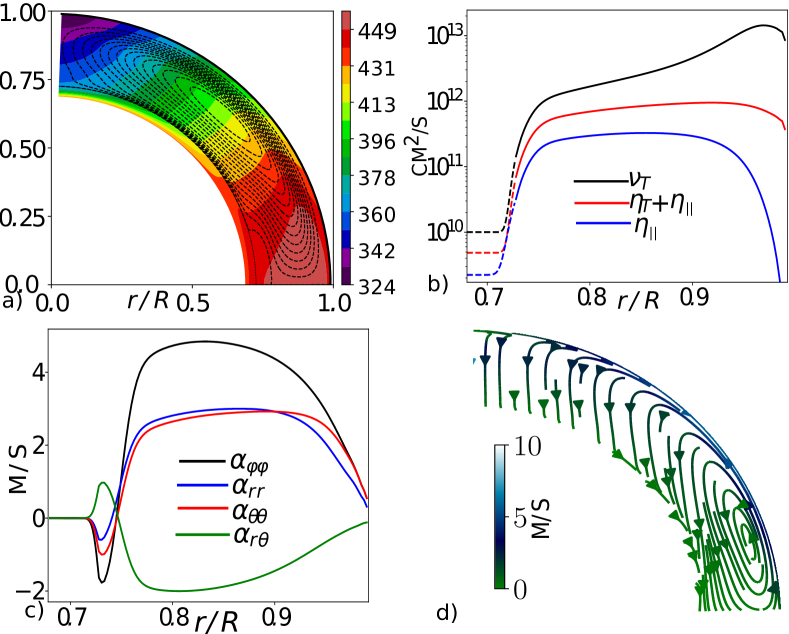
Figure 8: (a) Streamlines of meridional circulation and the angular velocity distribution; the magnitude of circulation velocity is of 13 m/s on the surface at the latitude of $45^{\circ}$. (b) Radial profiles of $\eta_{\rm T}+\eta_{||}$, the rotationally induced part $\eta_{||}$, as well as $\nu_{\rm T}$. (c) Radial profiles of the $\alpha$ tensor at $45^{\circ}$ latitude. (d) Streamlines of effective drift velocity from magnetically affected pumping and meridional circulation. Reproduced by permission from Pipin (2022).

Figure 8 shows profiles of the basic turbulent effects and large-scale flow distributions for the nonmagnetic case. The amplitude of the meridional circulation on the surface is about $13\,{\rm m}\,{\rm s}^{-1}$. In the lower part of the convection zone, the equatorward flow is about $1\,{\rm m}\,{\rm s}^{-1}$. The angular velocity profile is in agreement with helioseismology data.

Interestingly, the stagnation point of the meridional circulation is near the lower boundary of the subsurface shear layer, i.e., at $r=0.9\,R$. This is in agreement with observations of Hathaway (2012) and the helioseismic inversions of Stejko et al (2021). The structure of meridional circulation and turbulent pumping promotes an effective equatorward drift of the toroidal magnetic field below the subsurface shear layer; see Fig. 8(d).

6.2 Parker–Yoshimura dynamo waves and extended cycle

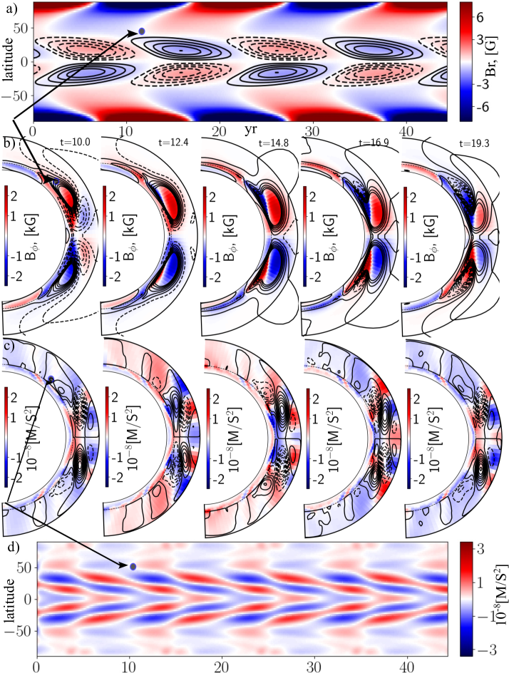
Figure 9: a) The surface radial magnetic field evolution (color image) and the toroidal magnetic field at $r=0.9R$ (contours in range of $\pm$1kG); b) snapshots of the magnetic field distributions inside the convection zone for half dynamo cycle, color shows the toroidal magnetic field and contours show streamlines of the poloidal field; c) snapshots of the dynamo induced variations of zonal acceleration (color image) and streamlines of the meridional circulation variations (contours); d) variations of zonal velocity acceleration at the surface. This Figure was prepared using the data of the dynamo model of PK19.

The dynamo shown in Fig. 9 demonstrates the numerical solution of the dynamo system including Eqs. (34) and (44)–(46). The time latitude diagrams of the surface radial magnetic field and the toroidal magnetic field in the upper part of the convection zone show agreement with observations of the evolution of the large-scale magnetic field of the Sun (Hathaway, 2015; Vidotto et al, 2018, see also the review of Righmire in this volume). The dynamo waves propagate to the surface- and equatorward. The radial direction of propagation follows the Parker–Yoshimura rule because of the positive sign of the $\alpha$ effect in the main part of the convection zone and a positive latitudinal shear. It is noteworthy that at high latitudes, the model shows another dynamo wave family which propagates poleward along the convection zone boundary. This family follows the Parker–Yoshimura rule as well. Further we will see that the latitudinal shear plays a dominant role in this dynamo model and perhaps in the solar dynamo as well (see also Cameron and Schüssler, 2015). The latitudinal drift of the toroidal magnetic field in this model results from turbulent pumping and meridional circulation; see Fig8(d). The GCD simulations of Warnecke, 2018; Warnecke et al, 2021 show the crucial role of turbulent pumping in the solar type dynamo model, as well. The extended mode of the dynamo cycle is another feature of their model. The toroidal magnetic dynamo wave starts at the bottom of the convection zone at around 50^∘ latitude (see the marks in Fig. 9). It disappears near the solar equator after a full dynamo cycle. On the surface, the extended mode of the solar cycle is seen in the radial magnetic field evolution, in the torsional oscillations of zonal flow, and in the variations of the meridional circulation as well (Getling et al, 2021). The origin of the extended mode of the dynamo cycle is due to the distributed character of the large-scale dynamo and the interaction of the global dynamo modes, where the low order dynamo modes, e.g., dipole and octupole modes, are mainly generated in the deep part of the convection zone. The high order modes are predominantly generated in the near surface level. The phase difference between the models results in a dynamo mode of the extended length (Stenflo, 1992; Obridko et al, 2021).

6.3 Torsional oscillations

Solar zonal variations of the angular velocity (“torsional oscillations”) were discovered by Howard and Labonte (1980). Since that time it was found that torsional oscillations represent a complicated wave-like pattern which consists of alternating zones of accelerated and decelerated plasma flows (Snodgrass and Howard, 1985; Altrock et al, 2008; Howe et al, 2011). Ulrich (2001) found two oscillatory modes of these variations with periods of 11 and 22 years. Torsional oscillations were linked to ephemeral active regions that emerge at high latitudes during the declining phase of solar cycles, but represent the magnetic field of the subsequent cycle (Wilson et al, 1988). It is interesting that in their original paper, Howard and Labonte (1980) conjectured that the solar torsional oscillation can shear magnetic fields and induce the dynamo cycle. This idea was further elaborated upon in a number of papers. However, the idea looks unreasonable because it conflicts with Cowling’s theorem. Also, the magnitude of the torsional oscillations of $3$–$6\,{\rm m}\,{\rm s}^{-1}$ is too small in comparison with the magnitude of the magnetic field generated by a dynamo. The first papers by Schuessler (1981) and Yoshimura (1981) suggested that the 11-year solar torsional oscillation can be explained by the mechanical effect of the Lorentz force. The double frequency of the zonal variation results from the $B^{2}$ modulation of the large-scale flow due to the dynamo activity. On the basis of a flux-tube dynamo model, Schuessler (1981) used the simple estimated of a large-scale Lorentz force and found both the 11 and 22 year mode of the torsional oscillations. This result was further elaborated upon by Kleeorin and Ruzmaikin (1991). The further development of the mean-field theory of the solar differential rotation showed that, in addition to the large-scale Lorentz force, the dynamo induced $B^{2}$ modulation of the turbulent angular momentum fluxes is also an essential source of the torsional oscillations (Rüdiger and Kitchatinov, 1990; Kitchatinov et al, 1994; Kleeorin et al, 1996; Küker et al, 1996; Rüdiger et al, 2012). Global convective dynamo simulations (e.g., Beaudoin et al, 2013; Käpylä et al, 2016a; Guerrero et al, 2016) confirmed this conclusion. The strength of the solar torsional oscillations is more than two orders of magnitude less than the differential rotation. It looks like the theory of the torsional oscillations can be constructed using perturbative approximations. Models of this type (see, e.g., Tobias 1996; Covas et al 2000; Bushby and Tobias 2007; Pipin 2015; Hazra and Choudhuri 2017) were inspired by results of Malkus and Proctor (1975). Yet, the constructed models are incomplete because they ignored the Taylor-Proudman balance, which is a key ingredient of solar differential rotation theory (see Kitchatinov 2013, also contribution of Hazra et al, this volume). Complete mean-field dynamo models, which take into accounts the Taylor-Proudman balance (hereafter TPB), were constructed by Brandenburg et al (1992), Rempel (2007), and PK19. Figure 9 shows variations of the zonal acceleration for our mean-field model in following the PK19 line of work. Similar to the results of helioseismology (Howe et al, 2011; Kosovichev and Pipin, 2019) and the results of Rempel (2007), snapshots of the model show that in the main part of the convection zone, the acceleration patterns are elongated along the rotation axis. This is caused by the Taylor-Proudman balance. Near the convection zone boundaries, these patterns deviate in the radial direction, which is in agreement with the above cited helioseismology results, as well. The given observation on the role of TPB shows the importance of the meridional circulation and the dynamo-induced heat transport perturbation (Spruit, 2003; Rempel, 2007) in the theory of torsional oscillations. This fact does not deny the importance of the large-scale Lorentz force and the magnetic modulation of the turbulent angular momentum transport. Results of Figures 9(b) and (c) show that the positive sign of the zonal acceleration propagates from high latitude bottom of the convection zone toward equator sticking to the equatorial edge of the dynamo wave. The torsional oscillation wave is accompanied by corresponding variations of the meridional circulation. These variations are induced by magnetic perturbations of the heat transport (see details in PK19). We emphasize that the given dynamo models also show overlapping magnetic cycles; see Fig. 9(b), similarly to what was originally proposed by Schuessler, 1981]. In this case, the $B^{2}$ effect of the dynamo on the heat transport and the TPB results in about 4 to 5 meridional circulation cells along latitude. This tracks the zonal variations of angular velocity, which are caused by the mechanical action of the large-scale Lorentz force and magnetic quenching of the turbulent stresses, from polar regions to the equator. PK19 found that the induced zonal acceleration is $\sim(2$–$4)\times 10^{-8}~{}$m s^-2, which is in agreement with the observational results of Kosovichev and Pipin (2019). However, the individual forces in the angular momentum balance such that the large-scale Lorentz force, the variations of the angular momentum transport due to meridional circulation, the inertial forces, and others are by more than an order of magnitude stronger than their combined action and can reach a magnitude of $\sim 10^{-6}~{}$m s^-2. Therefore, the resulting pattern of the torsional oscillations forms in nonlinear balance, which includes the forces driving the angular momentum transport, the TPB, and heat perturbations due to magnetic activity in the convection zone (see details in PK19).

7 Mean-field models based on the EMF obtained from DNS

Here we provide an example of how the mean-field theory is utilized as a tool for understanding what is going on (see Sect. 3.4). We discuss recent studies of mean-field dynamo models constructed based on the electromotive force (EMF) obtained from direct numerical simulation (DNS) of rotating stratified convection, especially focusing on “semi-global” models. The properties of solar and stellar convection, and the various methods for extracting the information of the EMF from DNS are also summarized.

7.1 Properties of solar and stellar convection

A quantitative physical description of solar and stellar dynamos, which should be the result of the nonlinear interaction of turbulent flows and magnetic fields, is a great challenge for us and constitutes a significant milestone on the long way to a full understanding of turbulence. Even with state-of-the-art supercomputers, it is impossible to numerically simulate solar and stellar convection and its interaction with the magnetic field and to observe/analyze numerical data in detail with realistic parameters. Therefore, to say with confidence that one has fully understood the solar and stellar dynamo problem, it should be necessary to find a universal law of magneto-hydrodynamic (MHD) turbulence, build a reliable sub-grid scale (SGS) turbulence model, and then reproduce the magnetic activities of the Sun and stars quantitatively in an integrated framework by numerical models with incorporating the SGS model. This is because fluid quantities that may be verified in future observations should include the meridional distributions of fluid velocity, vorticity, kinetic helicity, and thus the turbulence model constructed on the basis of these profiles (e.g., Hanasoge et al, 2016). Only when the correctness of the turbulence model is observationally validated should our understanding of the solar and stellar dynamos as a consequence of the turbulent dynamo process be completed. In the near future, a very exciting time may come when we will be able to test and verify various turbulence models under extreme conditions inside the solar and stellar interiors.

What physical characteristics should be taken into account when constructing a turbulence model of thermal convection in the Sun and stars? Let us summarize some essential features:

1. Extremely low dissipation: turbulent state with ${\rm Re}\gtrsim 10^{12}$, $\mbox{\rm Re}_{\rm M}\gtrsim 10^{8}$, and a large Pèclet number, ${\rm Pe}\sim 10^{6}-10^{9}$ (where ${\rm Pe}={\rm Re}\cdot{\rm Pr})$.

2. Huge separation of dissipation scales: ${\rm Pr}\sim 10^{-4}$–$10^{-7}$, ${\rm Pr_{M}}\sim 10^{4}$

3. Compressibility: high Mach number $\mathcal{O}(1)$ in the upper convection zone makes the convective motion compressible.

4. Anisotropy: spin of stars (i.e., Coriolis force in a rotating system) makes fluid motions anisotropic.

5. Inhomogeneity: density contrast of $10^{6}$ between top and bottom CZs results in multi-scale properties of fluid motion.

6. Non-locality: Radiative energy loss at the CZ surface (open system), allowing the growth of cooling-driven downflow.

In view of these features, it can be seen that the characteristics of thermal convection operating inside the Sun and stars are quite different from those of isotropic turbulence. Those can be considered to some extent in DNS even with the current computing performance, as listed under 3–6, while the others, (items 1 and 2) are unreachable with current grid-based simulations. It should be emphasized, however, that higher resolution simulations using state-of-the-art supercomputers is a classical way forward in turbulence research, and the knowledge obtained from such studies in unexplored low-dissipation regimes will greatly expand the horizon of our understanding of turbulence (e.g., Kaneda et al, 2003; Hotta and Kusano, 2021). Moreover, if sufficient scale separation between the turbulent and mean fields is ensured and the inertial range of the turbulent cascade is captured appropriately, there is the possibility that the evolution of mean-field components, such as large-scale flow and large-scale magnetic field, can be approximately reproduced even by simulations with enhanced dissipation compared to the actual solar and stellar values (e.g., Ossendrijver, 2003). It should be remembered, however, that in spite of the rapid increase in computing power, some rather basic questions about the solar dynamo still remain, for example the equatorward migration of the sunspot belts and the formation of sunspots themselves.

7.2 Semi-global simulation of rotating stratified convection

On our way toward a reliable SGS turbulence model for solar and stellar interiors, numerical models of convection and its dynamo should be studied, while keeping the characteristic features of solar and stellar convection, as listed under items 3–6 above, in mind. It should be noted that the underlying necessity for numerical modeling is an important component of earlier studies that applied mixing-length type concepts to the dynamo theory, which never successfully explained the magnetic activities of the Sun and stars (e.g., Brandenburg and Tuominen, 1988).

In recent years, significant progress has been made in GCD simulations (e.g., Browning et al, 2006; Ghizaru et al, 2010; Käpylä et al, 2012; Masada et al, 2013; Fan and Fang, 2014; Augustson et al, 2015; Hotta et al, 2016; Warnecke, 2018), there is also a growing effort to extract the information of turbulent transport processes from so-called “semi-global” (or local model) MHD convection simulations with the aim of quantifying the dynamo effect of rotational stratified convection (e.g., Brandenburg et al, 1990, 1996; Nordlund et al, 1992; Brummell et al, 1998, 2002; Ossendrijver et al, 2001; Käpylä et al, 2006a, 2009b; Masada and Sano, 2014b, a, 2016; Bushby et al, 2018; Masada and Sano, 2022). A typical numerical setup of the semi-global model is shown in Fig. 10 schematically. In this setting, the gas is gravitationally stratified in the vertical direction, while periodicity is assumed in the horizontal directions. The governing equations (mostly compressible MHD equations) are solved in a rotating Cartesian frame, and the rotation axis is usually set to be parallel or anti-parallel to the gravity vector. Several studies have simulated the model with the tilt of the rotation axis with respect to the gravity vector, and the latitudinal dependence of the convection has been investigated (e.g., Ossendrijver et al, 2001; Käpylä et al, 2004, 2006a).

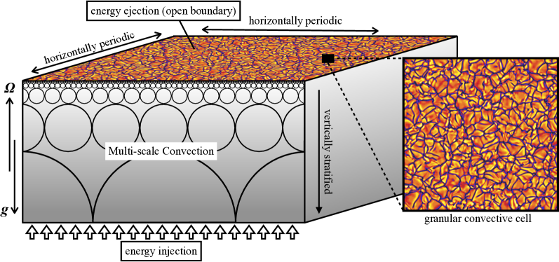
Figure 10: Numerical setup typical for semi-global simulation of rotating stratified convection. Since the CZs of the Sun and stars are strongly stratified, there is a large separation of time scales from minutes (upper CZs) to months (bottom CZs).

7.3 Extraction of information of dynamo effects

In the semi-global studies, four-types of approaches have been used typically to extract the information of dynamo effects veiled in the convective motion. The starting point of all the four methods is common, the decomposition of the flow field (${\bm{U}}$) and magnetic field (${\bm{B}}$) into a spatially large-scale, slowly-varying mean-component, and a small-scale, rapidly varying fluctuating component, as introduced in § 1, i.e., ${\bm{U}}=\overline{{\bm{U}}}+{\bm{u}}$ and ${\bm{B}}=\overline{{\bm{B}}}+{\bm{b}}$, where the lower-case represent the fluctuating component and the overbars denote the mean component. In the case of a semi-global model, a temporal and horizontal average is often used for deriving the mean component. Then, the equation of mean-field electrodynamics can be derived

$$\frac{\partial\overline{\bm{B}}}{\partial t}=\nabla\times(\overline{{\bm{U}}}\times\overline{{\bm{B}}}+\overline{\mathbfcal{E}}-\eta\nabla\times\overline{{\bm{B}}})\;,$$ (52)

where $\overline{\mathbfcal{E}}=\overline{{\bm{u}}^{\prime}\times{\bm{b}}^{\prime}}$ is the mean electromotive force (EMF) due to the fluctuation of the flow and the magnetic field. The mean EMF can be described as a power series about the large-scale magnetic component and its derivatives as

$$\overline{\mathbfcal{E}}=\overline{{\bm{u}}\times{\bm{b}}}={\bm{\alpha}}\cdot\overline{{\bm{B}}}+{\bm{\gamma}}\times\overline{{\bm{B}}}-{\bm{\beta}}\cdot(\nabla\times\overline{{\bm{B}}})+\cdots\;,$$ (53)

where ${\bm{\alpha}}$ represents (tonsorial form of) the $\alpha$-effect, ${\bm{\gamma}}$ is the turbulent pumping, and ${\bm{\beta}}$ denotes the turbulent diffusion.

To obtain the information of the dynamo coefficients, such as ${\bm{\alpha}}$, ${\bm{\gamma}}$, and ${\bm{\eta}_{T}}$, from the MHD convection simulation, there are the following four methods (see general discussion in Sect. 3.3):

1. Methods based on results of analytical theories, e.g., SOCA (or first-order smoothing approximation, FOSA) expressions

2. Imposed-field method

3. Test-field method

4. The multi-dimensional regression method based on the dynamo generated magnetic field

Method (i) involves the the estimation of dynamo coefficients based on results of analytical theory. It also exploit the mixing-length approximation in final results. There, the distributions of, for example, the fluctuating components of the convection velocity (${\bm{u}}$), vorticity (${\bm{\omega}}=\nabla\times{\bm{u}}$), and the resulting kinetic helicity ($\mathcal{H}={\bm{\omega}}\cdot{\bm{u}}$), are directly extracted from the simulation results and used to reconstruct the turbulent $\alpha$ and $\beta$ via their analytic forms, derived under SOCA, such as Eq. (16) and $\beta=(\tau/3)\overline{{\bm{u}}^{2}}$, where $\tau$ is the correlation time of the turbulence and is often replaced by the convective turnover time, $\tau_{c}$. Note that anisotropy effects are often neglected in the expressions above, but see Brandenburg and Subramanian (2007), who included them.

Method (ii) is mainly used in the analysis of the numerical results without self-sustained magnetic field. In this method, a uniform external magnetic field is imposed as the mean component to the computational domain, artificially. The $\alpha$ effect and turbulent pumping are then inferred from $\overline{\mathbfcal{E}}=\overline{{\bm{u}}\times{\bm{b}}}$ by directly calculating from simulation data

$$\alpha=\overline{\mathbfcal{E}}\cdot\overline{{\bm{B}}}/\overline{{\bm{B}}}^{2}\;,\quad\mbox{\boldmath$\gamma$}{}=-\overline{\mathbfcal{E}}\times\overline{{\bm{B}}}/\overline{{\bm{B}}}^{2}\;.$$ (54)

Furthermore, one might be tempted to compute $\eta_{\rm t}=\overline{\mathbfcal{E}}\cdot{\overline{\bm{J}}}/(\mu_{0}{\overline{\bm{J}}}^{2}$), but this would assume that ${\overline{\bm{J}}}\cdot{\overline{\bm{B}}}$ is vanishing, which is generally not the case for $\alpha$-effect dynamos; see Hubbard et al (2009) for details.

Method (iii) utilizes a so-called test field, as introduced by Schrinner et al (2005, 2007) for the spherical case and Brandenburg et al (2008) for the Cartesian case, allowing for scale dependence. In this method, the evolution equation of ${\bm{b}}^{\prime}_{\rm T}$, the fluctuating component of the test field ${\bm{B}}_{\rm T}$, which are passive to the velocity field taken from the simulation, is solved additionally to the basic (MHD) equations. From the linear evolution of the test-field, the mean EMF is evaluated and then the full set of turbulent transport coefficients can be obtained. For example, in the case without the large-scale flow, the test-field equation is, for ${\bm{b}}_{\rm T}$,

$$\frac{\partial{\bm{b}}_{\rm T}}{\partial t}=\nabla\times({\bm{u}}\times{\bm{B}}_{\rm T}+{\bm{u}}\times{\bm{b}}_{\rm T}-\overline{{\bm{u}}\times{\bm{b}}_{\rm T}}-\eta\nabla\times{\bm{b}}_{\rm T})\;,$$ (55)

with a chosen test field ${\bm{B}}_{\rm T}$ while taking ${\bm{u}}$ from the MHD simulation. The original method does not work in cases when magnetic fluctuations are driven through an artificially added electromotive force. In such cases, one needs to use a more general nonlinear method explored by Rheinhardt and Brandenburg (2010) and Käpylä et al (2022). Theses magnetically driven systems are also examples where the imposed-field method gives reliable results in two dimensions with volume averaged mean fields, where no turbulent diffusion can act.

Method (iv) can be used only in the analysis of the numerical results with self-sustained magnetic fields. Since the fluctuating and mean components are all known quantities in such simulations, the mean emf, $\overline{\mathbfcal{E}}=\overline{{\bm{u}}\times{\bm{b}}}$, and the mean magnetic component, $\overline{{\bm{B}}}$, can be directly calculated from the simulation data. Then, the mean profiles of dynamo coefficients are inferred based on a fitting procedure via the relationship,

$$\mathcal{E}_{i}=\alpha_{ij}\overline{B}_{j}+\epsilon_{ijk}\gamma_{j}\overline{B}_{k}+\mbox{higher derivative terms}\;.$$ (56)

Given $\mathcal{E}_{i}$ and $\overline{B}_{i}$ which are calculated from simulation data, and then find $\alpha_{ij}$ and $\gamma_{i}$ such that the residual of Eq. (56) is minimized. In the equation above, the contributions from the derivatives of the mean magnetic component to the mean emf are neglected (see, e.g., Racine et al, 2011; Simard et al, 2013, 2016; Shimada et al, 2022, for the fitting based analysis of the dynamo coefficient with including the contribution from the first-order derivative of the mean magnetic component). As we have mentioned in Sect. 3.3, the results of Warnecke et al (2018) show that the TFM is more accurate compared to the regression method in obeying Eq. (56); see the detailed comparison in above cited paper.

In all cases, however, the first (and often higher) derivative terms are of the same order as the first term and can therefore not be neglected. This was already done in the work of Brandenburg and Sokoloff (2002), who typically found small diffusion coefficients in the cross-stream direction. This, however, turned out to be a shortcoming of the method and has not been borne out by more advanced measurements (Karak et al, 2014).

7.4 Transport coefficients from semi-global turbulence simulations

Here, we briefly review the results of previous semi-global simulations, with a particular focus on the studies that have been dedicated for extracting information about dynamo coefficients.

Brandenburg et al (1990), hereafter B90, performed turbulent 3-D magneto-convection simulations under the influence of the rotation for the semi-global model whose depth is equivalent to about one pressure scale height. They found that, due to the effect of the rotation, a systematic separation of positive and negative values of the kinetic helicity was developed in the vertical direction of the CZ, i.e., in the upper CZ, negative (positive) helicity in the northern (southern) hemisphere, while positive (negative) helicity in the northern (southern) hemisphere. Using the imposed field method, they evaluated the magnitude of the turbulent $\alpha$-effect with anisotropic properties as $\alpha_{V}/(\tau\mathcal{H})\sim\mathcal{O}(0.1)$ and $\alpha_{H}/(\tau\mathcal{H})\sim\mathcal{O}(0.01)$, where $\mathcal{H}={\bm{\omega}}\cdot{\bm{u}}$ and $\overline{\mathbfcal{E}}=\alpha_{\rm H}\overline{\bm{B}}_{\rm H}+\alpha_{\rm V}\overline{\bm{B}}_{\rm V}$. It is interesting to note that these values are about one to two orders of magnitude smaller than $\alpha\sim\Omega d$, which is the estimation based on the mixing-length theory. Additionally, it was also suggested that the magnetic helicity showed a similar depth variation, but the sign was opposite to that of the kinetic helicity.

While $\alpha_{\rm H}$ had the expected sign (opposite to that of the kinetic helicity), $\alpha_{\rm V}$ was found to have the ‘wrong’ sign (same as that of the kinetic helicity). Such a result was subsequently also obtained by Ferriere (1993). The theoretical possibilities for such effects should be studied further. For example, Rüdiger and Pipin (2000) found that large-scale shear can affect both the sign of the $\alpha$ effect and kinetic helicity in magnetically driven compressible turbulence in such a way that they have the same sign, e.g., for Keplerian accretion disks. These ideas were also applied to understanding the finding of a negative $\alpha$ effect in stratified accretion disk simulations (Brandenburg, 1998).

Ossendrijver et al (2001) also performed the semi-global simulation with a similar model as B90. They showed that, even in the regime where the condition justifying the FOSA (or SOCA) is not satisfied, i.e., in the situation where ${\rm St}=u_{\rm rms}\tau/d\gtrsim 1$ and $Re>1$, the kinetic helicity was clearly separated into positive and negative values at the lower and upper CZs when taking temporal average of the convective motion over sufficiently long time. Using the imposed field method, they also measured the magnitude of the turbulent $\alpha$-effect and obtained similar values to B90 in terms of $\alpha_{H}$ and $\alpha_{V}$. The rotational dependence of the $\alpha$-effect was also investigated in this work for the first time. They showed that, in the larger ${\rm Co}$ regime, the $\alpha_{V}$ underwent a rotational quenching, while the $\alpha_{H}$ was saturated, where Co is the Coriolis number [see Eq. (37)]. The turnover time was defined, in this work, as $\tau=d/u_{\rm rms}$. While the depth-dependence or rotational dependence of the $\alpha$, which was obtained from the simulation, agreed, to some extent, with a theoretical model based on the mixing-length theory (Rüdiger & Kitchatinov 1993), their amplitudes were one to two orders of magnitude smaller than those predicted from the theoretical model. Noteworthy, the critical threshold of the $\alpha$ effect parameter in mean-field dynamo models (see Sect. 6.1) is about same magnitude less than the mixing-length models of the solar convection zone predicts; see Sect. 6.

In Käpylä et al (2004, 2006a), additionally to the rotational dependence, the latitudinal dependence of the turbulent $\alpha$-effect was studied in the semi-global convection simulations with varying the inclination of the rotation axis with respect to the gravity vector. With the imposed field method, they found that, for slow and moderate rotation with ${\rm Co}<4$, the latitudinal dependence of the $\alpha$ followed $\cos\theta$ profile with a peak at the pole (see also, Egorov et al, 2004), while, in the rapid rotation regime with ${\rm Co}\approx 10$, it rather peaked much closer to the equator at $\theta\simeq 30^{\circ}$. Additionally, the vertical profile of the $\alpha$ directly evaluated from simulation was found to be qualitatively consistent with analytic expression derived under the FOSA even when changing the latitude. A practical application of these results was the development of a kinematic mean-field solar dynamo model in Käpylä et al (2006b). In it, the rotation profile deduced from the helioseismic observation and the meridional profiles of the $\alpha$-effect and turbulent pumping obtained with the semi-global simulation of Käpylä et al (2006a) are integrated into the framework of the $\alpha$–$\Omega$ dynamo, and then the solar dynamo mean-field model was constructed. It is interesting that their kinematic dynamo model correctly reproduced many of the general features of the solar magnetic activity, for example realistic migration patterns and correct phase relation.

The existence of large-scale dynamo, i.e., self-excitation of the mean magnetic component, in rigidly-rotating convection was demonstrated for the first time in the semi-global simulation by Käpylä et al (2009b). By changing the angular velocity, they showed that the large-scale dynamo could be excited only when the rotation is rapid enough, i.e., ${\rm Co}\gtrsim 60$, with Eq. (37) as the definition of ${\rm Co}$ which is same as that used in Ossendrijver et al (2001) and Käpylä et al (2006a); see, e.g., Tobias et al (2008) and Cattaneo and Hughes (2006), and Favier and Bushby (2013), for unsuccessful large-scale dynamo in rigidly-rotating convection probably due to slow rotation, and/or short integration time. From the measurements of the turbulent $\alpha$-effect and the turbulent diffusivity by the TFM, they also suggested that while the magnitude of the $\alpha$-effect stayed approximately constant as a function of rotation, the turbulent diffusivity decreased monotonically with increasing the angular velocity, resulting in the excitation of the large-scale dynamo in the higher ${\rm Co}$. The reliability of the dynamo coefficients extracted with the test-field method from the simulation was validated with the one-dimensional mean-field dynamo model in which the test-field results for $\alpha$ and $\beta$ were used as input parameters by studying the excitation of the large-scale magnetic field at the linear stage. Note that the oscillatory properties of the large-scale dynamo in rigidly-rotating convection and its possible relationship with $\alpha^{2}$ dynamo mode with inhomogeneous $\alpha$ profile were also found in Käpylä et al (2013); see, e.g., Baryshnikova and Shukurov (1987) and Mitra et al (2010b) for the oscillatory $\alpha^{2}$ dynamo.

7.5 Mean-field dynamo models linked with DNSs

Weakly-stratified Model

Below we review recent mean-field dynamo models linked with semi-global MHD convection simulations, where the large-scale dynamo is successfully operated; see Masada and Sano (2014a, b, 2016, 2022) for a series of numerical studies.

While Käpylä et al (2009b, 2013) were the first to demonstrate that rigidly-rotating convection can excite the large-scale dynamo as reviewed above, their simulation model was a so-called “three-layer polytrope” consisting of top and bottom stably-stratified layers and the CZ in between them. Therefore, it was suspected for a while that the essential factor for the successful large-scale dynamo observed there might be the presence of the stably-stratified layer assumed in their model rather than the rapid rotation (e.g., Favier and Bushby, 2013). To pin down the key requirement for the large-scale dynamo, the impact of the stably-stratified layers on the large-scale dynamo was studied in Masada and Sano (2014b), hereafter MS14a, in which two-types of semi-global models with and without stably-stratified layers are compared with the same control parameters and the same grid spacing. It was found in this study that a large-scale dynamo was successfully operated even in the model without the stably-stratified layer, and confirmed that the key requirement for it should be a rapid rotation if we evolved the simulation for a sufficiently long time than the ohmic diffusion time. Note that a relatively weak density stratification (the density contrast between the top and bottom CZs is about $10$) was assumed in the simulation model employed in this study as well as Käpylä et al (2009b, 2013).

With these results, Masada and Sano (2014a), hereafter MS14b, explored the mechanism of the large-scale dynamo operated in the rigidly-rotating stratified convection by linking the mean-field (MF) dynamo model with the DNS. In this study, the FOSA based approach was adopted in the MF modeling. The mean vertical profiles of the kinetic helicity and root-mean square velocity were directly extracted from the simulation data and then the vertical profiles of the turbulent $\alpha$, turbulent pumping ($\gamma$) and turbulent diffusivity ($\beta$) were reconstructed according to the analytic expressions of

$$\alpha(z)=-\tau_{c}(\overline{u_{z}\partial_{x}u_{y}}-\overline{u_{z}\partial_{y}u_{x}})\;,\ \ \ \gamma(z)=-\tau_{c}\partial_{z}\overline{(u_{z})^{2}}\;,\ \ \ \beta(z)=\tau_{c}\overline{(u_{z})^{2}}\;,$$ (57)

in anisotropic forms of dynamo coefficients under the FOSA (e.g., Käpylä et al, 2006a). Although recent numerical studies indicate that the small-scale current helicity, i.e., ${\bm{j}}\cdot{\bm{b}}$, is important for the $\alpha$-effect when the magnetic field is dynamically important (Pouquet et al, 1976; Brandenburg and Subramanian, 2005b), its contribution was ignored in this study. As the correlation time $\tau_{c}$, the convective turnover time defined by $\tau=H_{\rho}(z)/u_{\rm rms}$ was chosen there ($H_{\rho}$ is the density scale-height as a function of the depth). By solving one-dimensional MF $\alpha^{2}$ dynamo equation in which these profiles were used as input parameters, i.e.,

$$\frac{\partial\overline{\bm{B}}_{h}}{\partial t}=\nabla\times(\overline{\mathbfcal{E}}-\eta\nabla\times\overline{{\bm{B}}}_{h})\;,$$ (58)

with

$$\overline{\mathbfcal{E}}=\alpha(z)\overline{\bm{B}}_{h}+\gamma(z){\bm{e}}_{z}\times\overline{\bm{B}}_{h}-\beta(z)\nabla\times\overline{\bm{B}}_{h}\;,$$ (59)

the time-depth diagram for the mean (horizontal) magnetic component ($\overline{\bm{B}}_{h}$) was obtained. In Fig. 11, we show $\overline{B_{x}}(z,t)$ for the MF model (panels (b)) and its DNS counterpart (panels (a)). Note that, for ensuring the saturation of the magnetic field growth, the quenching effect was also taken into account. Since the DNS results were quantitatively reproduced by the MF $\alpha^{2}$ dynamo, MS14b concluded that the large-scale magnetic field organized in the rigidly-rotating turbulent convection was a consequence of the oscillatory $\alpha^{2}$ dynamo.

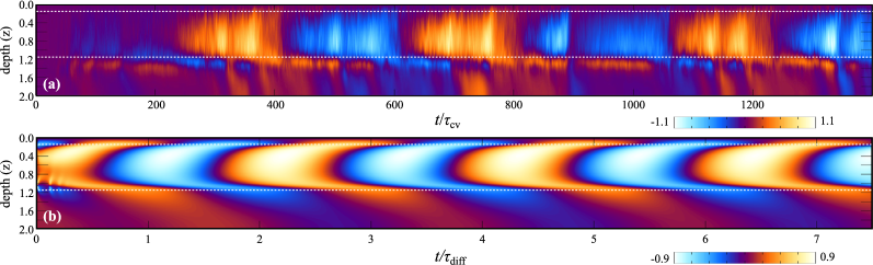
Figure 11: Time-depth diagram $\overline{B}_{x}(z,t)$ for the MF model (panel (b)) and its DNS counterpart (panel (a)). For DNS result, the horizontal average of the magnetic field is shown. The orange and blue tones represent positive and negative $\overline{B}_{x}$ in units of $B_{\rm cv}\equiv(\overline{\rho{\bm{u}}^{2}})^{1/2}$. Time is normalized by $\tau_{c}$. Note that $\overline{B}_{y}$ shows a similar cyclic behavior with $\overline{B}_{x}$ yet with a phase delay of $\pi/2$; see MS14a,b for details.

Reproducing the DNS results with mean-field models using coefficients from the original DNS is an important verification of the whole approach. This has been done on many occasions in the past; see, for example, the work by Gressel (2010) and Warnecke et al (2021).

A strongly stratified model

In MS14a,b, a weakly-stratified model, in which the density contrast between top and bottom CZs is about $10$, was adopted. However, the actual Sun has very strong stratification with a density contrast of $\sim 10^{6}$ between top and bottom CZs, resulting in a large segregation of time scales from minutes to months. Aiming at the application to solar and stellar interiors, Masada and Sano (2016), hereafter MS16, performed a convective dynamo simulation in a strongly stratified atmosphere with a density contrast of $700$ in a semi-global setup. Due to the strong solar- and stellar-like density stratification, multi-scale convection with a strong up-down asymmetry, i.e., slower and broader upflow regions surrounded by a network of faster and narrower downflow lanes, was developed in this simulation, as shown in Fig. 12(a). Even in such a situation, a large-scale dynamo was found to operate. As shown in Fig. 12(b), the mean magnetic field components observed there showed a time–depth evolution similar to that seen in the weakly-stratified model (MS14a,b), suggesting that an oscillatory $\alpha^{2}$ dynamo is responsible for it. It was intriguing that, in addition to the mean horizontal component, the large-scale structures of the vertical magnetic field were spontaneously organized at the CZ surface in the case of the strongly stratified atmosphere, as shown in Fig. 13.

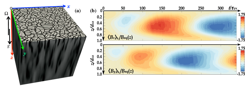
Figure 12: (a) 3-D view of the strongly stratified convection (for the progenitor run without rotation). The black (gray) tone denotes downflows (upflows). (b) Time-depth diagrams for $\overline{B}_{x}$ and $\overline{B}_{y}$. The normalization is the equipartition field strength, $B_{\rm eq}\equiv(\overline{\rho{\bm{u}}^{2}})^{1/2}$. In MS16, a one-layer polytrope with a super-adiabaticity of $\delta\equiv\nabla-\nabla_{\rm ad}=1.6\times 10^{-3}$ was used; see MS16 and MS22 for details.

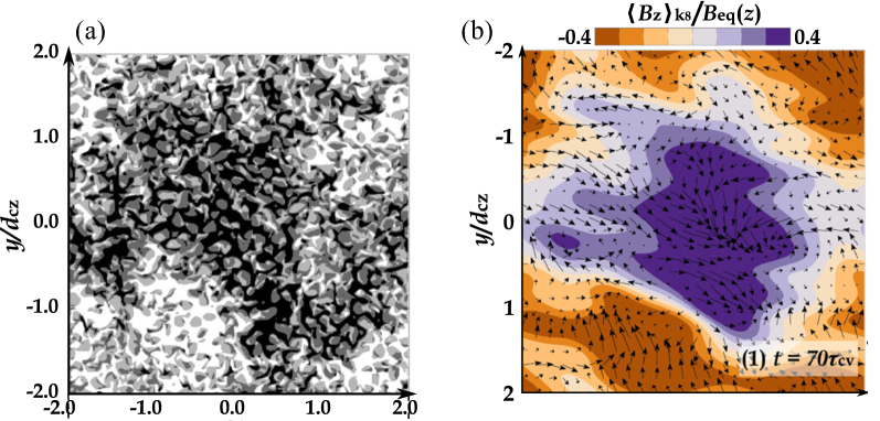
Figure 13: Snapshots for (a) the horizontal distribution of $B_{z}$ at the CZ surface, and (b) its Fourier filtered image. In panel (b), the small-scale structures with $k/k_{c}\gtrsim 8$ are eliminated for casting light on the large-scale pattern ($k$ is the wavenumber and $k_{c}=2\pi/L_{h}$ with the horizontal box size $L_{h}$).

A possible physical origin of such surface magnetic structure formation is the negative magnetic pressure instability (NEMPI; see § 8 for details). NEMPI is a mean-field process in the momentum equation, where the Reynolds and Maxwell stresses attain a component proportional to the square of the mean magnetic field, which acts effectively like a negative pressure by suppressing the turbulent pressure. Since its growth rate becomes larger for stronger density stratification (e.g., Jabbari et al, 2014), one can imagine that it may play an important role in organizing sunspot-like large-scale magnetic field structures in the upper part of the solar CZ. Although its presence has been confirmed numerically in forced MHD turbulence (e.g., Brandenburg et al, 2011; Warnecke et al, 2013), it does not play a significant role in organizing the surface magnetic structure seen in MS16 because of their relatively rapid rotation; $\mbox{\rm Ro}=0.02$ was assumed there, while, according to Losada et al (2012), $\mbox{\rm Ro}\gtrsim 5$ is required to excite the NEMPI.

The large-scale structure of the vertical magnetic field observed in MS16 is similar to that observed in the large-scale dynamo by forced turbulence in a strongly stratified atmosphere (Mitra et al, 2014; Jabbari et al, 2016). This implies that there would be an as-yet-unknown mechanism for the self-organization of large-scale magnetic structures, which would be inherent in a strongly stratified atmosphere.

In Masada and Sano (2022), hereafter MS22, with varying angular velocity as a control parameter, the rotational dependence of the large-scale dynamo was explored in a series of DNSs of rigidly-rotating convection. They linked its cause through MF dynamo models with DNSs where a strongly stratified polytrope was adopted as a model of the convective atmosphere, as in MS16.

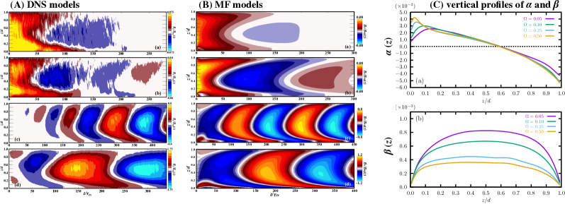
Figure 14: Time-depth diagrams of $\overline{B}_{x}$ for (A) DNS models and (B) MF models. (C) Vertical profiles of the turbulent $\alpha$-effect (top) and turbulent diffusivity $\beta$ (bottom) which are reconstructed with the analytic expressions of Eq. (57) from the information, such as kinetic helicity and rms velocity, directly extracted from DNSs.

In Fig. 14(a), DNS results are shown where a time-depth diagram of $\overline{B}_{x}$ is depicted for models with different values of Co. While in the slowly rotating model with low Co, the large-scale magnetic component fails to grow, it is found to be spontaneously organized in the rapidly-rotating models with high Co. It was found from DNS that the large-scale dynamo was excited when $\mbox{\rm Co}\gtrsim\mbox{\rm Co}_{\rm crit}$, where $\mbox{\rm Co}_{\rm crit}$ is the critical Coriolis number in the range $25\lesssim\mbox{\rm Co}_{\rm crit}\lesssim 80$, with Eq. (37) as the definition of the Coriolis number. It is remarkable that $\mbox{\rm Co}_{\rm crit}$, which determines the success or failure of the large-scale dynamo, was almost the same – independent of the density contrast (see Käpylä et al, 2009b) or the geometry of the simulation model (see, e.g., Käpylä et al, 2012; Warnecke, 2018, for $\mbox{\rm Co}_{\rm crit}$ in the global simulations); see MS22 for the quantitative comparison between models.

To explore the underlying mechanism of the rotational dependence of the large-scale dynamo, the influence of the rotation on the turbulent transport coefficients was also studied in MS22 with the FOSA-based approach similar to that adopted in MS14b. In Fig. 14(c), the vertical profiles of the turbulent $\alpha$ effect and turbulent diffusivity $\beta$ reconstructed with the analytic expressions of Eq. (57) were shown. It can be found that, as the spin rate increases, the turbulent diffusivity decreases significantly, but the profile of the $\alpha$ effect remains almost unchanged. This result suggested that the rotational dependence of the large- scale dynamo observed in MS22 may be primarily due to a change in the magnitude of the turbulent diffusion. In fact, this insight was confirmed by the evidence that the MF dynamo model with incorporating the dynamo coefficients shown in Fig. 14 reproduced quantitatively the result of the DNS; see Fig. 14(b) for the time-depth diagram of $\overline{B}_{x}$ obtained in the MF models with using different dynamo coefficients extracted from the corresponding DNSs.

MS22 concluded that the independence (dependence) of the turbulent $\alpha$ effect (turbulent diffusivity) on the rotation was the essence of the rotational dependence of the dynamo. This is not only the same as the conclusion obtained by Käpylä et al (2009b) from weakly-stratified convective dynamo simulations using the TFM, but also the same as that obtained by Shimada et al (2022) from global solar dynamo simulation with using the “self-sustained field method”. Although we don’t know whether the independence (dependence) of the $\alpha$-effect (turbulent diffusion) on the rotation, seen in these studies, is universal or not, it may give an important suggestion not only on the turbulence modeling but on the solar dynamo modeling.

8 Solar-stellar connections and questions beyond standard mean-field theory

The title of our review is “Turbulent processes and mean-field dynamo” Obviously, there are mean-field effects in turbulence that are not just of dynamo type, and the mean-field dynamo is not just related to the solar dynamo problem, but its relevance goes much beyond. Here, we highlight, just some effects, but we refer to the reviews of Käpylä et al (2023) for additional examples.

8.1 Origin of sunspots and active regions

An important goal in solar dynamo theory is to compute synthetic butterfly diagrams. The question then emerges from which depth to take the mean toroidal field, for example. The usual argument here is to invoke Parker’s theory of sunspot formation and to postulate that the field at some depth translates directly to one at the surface. This is critical because the final result depends on the assumed depth.

It is possible that sunspots are not deeply rooted, but are actually a surface phenomenon. No successful and self-consistent model of shallow formation of active regions or sunspots exists as yet. Noteworthy in this context is NEMPI, which is a mean-field theory of the Reynolds and Maxwell stresses. This theory is extremely successful in that its results agree remarkably well with direct numerical simulations (DNS). The problem is only that the effect is not strong enough to make real sunspots or active regions. Because of this remarkable agreement between theory and simulations, and because it is an important mean-field process, we shall discuss here a bit more detail.

The essence of the effect is the contribution of the turbulent hydromagnetic pressure to the horizontal force balance. The turbulent pressure is a small-scale effect, but it reacts to the large-scale magnetic field. As the magnetic field increases, it suppresses the turbulence locally, disturbing therefore the horizontal force balance. Although this large-scale magnetic field itself contributes with its own magnetic pressure to the horizontal force balance, the effect from the suppression of the turbulence is often stronger, so the net effect is a negative one. This is why the mean-field effect from a large-scale magnetic field is a negative effective magnetic pressure. This idea goes back to early work of Kleeorin et al (1989, 1996), who developed the mean-field theory for this effect.

In the beginning, it was not clear what kind of numerical experiments one could try to test the a negative effective magnetic pressure effect. The first mean-field simulations were done with a uniform horizontal magnetic field (Brandenburg et al, 2010). This led to the development of magnetic flux concentrations near the surface, but those began to sink downward as time went on. A similar effect was soon also seen in DNS (Brandenburg et al, 2011). The sinking of such structures was explained by the negative effective magnetic pressure: a positive magnetic pressure would lead to the rise of structures (Parker, 1967) while a negative one leads to a sinking. The sinking of magnetic structures had the side effect that the structures disappeared from the surface and became less prominent.

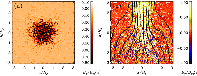
Figure 15: Cuts of $B_{z}/B_{\rm eq}(z)$ in the $xy$ plane at the top boundary ($z/H_{\rho}=\pi$) and the $xz$ plane through the middle of the spot at $y=0$. In the $xz$ cut, we also show magnetic field lines and flow vectors obtained by numerically averaging in azimuth around the spot axis. Adapted from Brandenburg et al (2013).

Subsequent experiments with a vertical field had a more dramatic effect on the general appearance of structures. Because the ambient field was vertical, the downflow had little effect on the magnetic flux concentrations themselves (Brandenburg et al, 2013). Fig. 15 shows the spontaneous development of a magnetic spot. Brandenburg et al (2013) found that NEMPI saturates slightly below equipartition value.

Most of the numerical experiments where done with forced turbulence, where one had explicit control over the degree of scale separation. For the results presented here $\mbox{\rm Re}_{\rm M}\sim 19$ and $\mbox{\rm Pr}_{\rm M}=0.5$. The value of $\mbox{\rm Re}_{\rm M}=u_{\rm rms}/\eta k_{\rm f}$ is very small because it is based on the forcing wavenumber $k_{\rm f}$, which is chosen to be large. Furthermore, $\mbox{\rm Pr}_{\rm M}$ is chosen to be less than unity, because NEMPI is not expected to work for $\mbox{\rm Pr}_{\rm M}\geq 14$. This is rather different in actual stellar convection, where the development of magnetic structures takes different shapes (Stein and Nordlund, 2012; Masada and Sano, 2016; Käpylä et al, 2016b).

8.2 Dynamo flux budget and impact of the surface activity on the deep dynamo

Following Cameron and Schüssler (2015) (hereafter, CS15, also see the chapter by Cameron & Schüssler) we now estimate the budget of the toroidal magnetic flux in the dynamo region. Using the Stokes theorem and the induction equation Eq. (34), we define the derivative of the toroidal magnetic field flux in the northern hemisphere of the Sun as

$$\frac{\partial\Phi_{\mathrm{tor}}^{\mathrm{N}}}{\partial t}=\oint_{\delta\Sigma}\left(\overline{\mathbf{U}}\times\mathbf{\overline{B}}+\bm{\mathcal{E}}\right)\cdot\mathrm{d\mathbf{l}},$$ (60)

where $\Phi_{\mathrm{tor}}^{\mathrm{N}}=\int_{\Sigma}\overline{B}_{\phi}\mathrm{dS}$, $\Sigma$ is the meridional cut of the northern hemisphere of the solar convection zone, $\delta\Sigma$ stands for the contour confining the cut and the differential $\mathrm{dl}$ is the line element of $\delta\Sigma$. The same can be written for the southern hemisphere flux $\Phi_{\mathrm{tor}}^{\mathrm{S}}$. Similarly to CS15, we use the boundary conditions, and we estimate the RHS of the Eq. (60) in the coordinate system which is co-rotating with angular velocity of the solar equator, $\overline{U}_{0\phi}=R\sin\theta\Omega_{0}$, and $\Omega_{0}$ the surface angular velocity at the equator,

$$\frac{\partial\Phi_{\mathrm{tor}}^{\mathrm{N}}}{\partial t} = \int_{0}^{\pi/2}\overset{\mathrm{I_{1}}}{\overbrace{\left(\overline{U}_{\phi}-\overline{U}_{0\phi}\right)\overline{B}_{r}\mathrm{r_{t}}}}\,\mathrm{d}\theta+\int_{\mathrm{r_{i}}}^{\mathrm{r}_{\mathrm{t}}}\overset{\mathrm{I_{2}}}{\overbrace{\left(\overline{U}_{\phi}^{(\mathrm{\frac{\pi}{2}})}-\overline{U}_{0\phi}\right)\overline{B}_{\theta}^{(\mathrm{\frac{\pi}{2}})}}}\mathrm{dr}$$

$$+ \int_{\mathrm{r_{i}}}^{\mathrm{r}_{\mathrm{t}}}\overset{\mathrm{I_{3}}}{\overbrace{\left(\mathcal{E}_{r}^{(\mathrm{0})}-\mathcal{E}_{r}^{(\mathrm{\frac{\pi}{2}})}\right)}}\mathrm{dr}+\int_{0}^{\pi/2}\overset{\mathrm{I_{4}}}{\overbrace{\left(\mathcal{E}_{\theta}^{(\mathrm{t)}}\mathrm{r_{t}}-\mathcal{E}_{\theta}^{(\mathrm{i})}\mathrm{r_{i}}\right)}}\mathrm{d}\theta$$

here, $r_{t}=0.99\,R$, $r_{i}=0.67\,R$, are the radial boundaries of the dynamo region. In compare to CS15 we have additional contributions in the budget equation. Figure 16 shows profiles of the kernels $I_{1-4}$ for the period of the magnetic cycle minimum. The estimations are based on results and parameters of the mean-field model presented above. Noteworthy, the south hemisphere should show the profiles of the opposite sign (see CS15). The results for $I_{1,4}$ qualitatively similar to CS15. This is because the mean-field model show the qualitative agreement with solar observations for the time latitude evolution of the surface radial magnetic field. The diffusive decay of the toroidal magnetic flux is captured as well because of the phase shift between evolution of the poloidal and toroidal magnetic field in dynamo model and presumably in the solar dynamo as well. The model show the sharp poleward increase of $I_{1}$. This effect produces the winding of the toroidal magnetic field from poloidal component by the latitudinal shear. The effect of the radial shear, $I_{2}$, has maximum near the bottom of the convection zone, where its magnitude is less than the $I_{1}$.

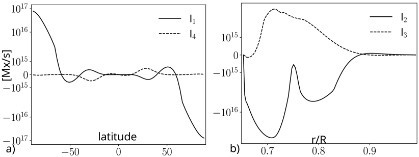
Figure 16: Estimation of contributions of the budget equation; see Eq. (8.2), for the time of cycle minimum.

Figure 17(a) shows the time evolution of the RHS contributions of Eq. (8.2). In our model the We see that $I_{2}$ has the same magnitude as $I_{1}$. Therefore, for the distributed mean-field dynamo model the latitudinal and radial shear produce equal effect on the net toroidal field in the bulk of the convection zone. This is different to applications of simple 1-D Babcock–Leighton dynamos to the solar observations as argued by CS15. Together with the fact of the poleward increase of $I_{1}$ it explain the relative success of correlation of the polar magnetic field strength and the magnitude of the subsequent magnetic cycle for the solar cycle prediction (Choudhuri et al, 2007).

Figure 17: (a) Time evolution of the RHS contributions of Eq. (8.2); (b) the dynamo models budget, black line show the standard mean-field model, green line – the budget which includes only the surface contributions ($I_{1,4}$) and the blue line shows the model with accounts of surface spot-like activity effects.

Figure 17(b) shows the budget of the toroidal flux generation rate ($I_{1}+I_{2}$) and loss rate($I_{3}+I_{4}$) for our dynamo model. The parameters of the budget are larger than those deduced by CS15 from solar observations. The difference is because of additional generation and loss terms. The budget which includes only the surface activity contributions (green line in Fig.17b) is less than the full case. Also, the magnitude of the generation rate by the latitudinal shear can be larger than in the solar observations because of difference in the latitudinal profiles of the surface radial magnetic field. We guess that in the dynamo model the radial magnetic field increase poleward steeper than in observations. This issue have to be studied further. Figure 17b shows the budget for another dynamo model which include the effects of the surface magnetic activity in form of bipolar magnetic regions. The model shows an increase of the toroidal field generation rate.

The above analysis shows the importance of surface activity for the dynamo model and perhaps for the solar dynamo as well. Sunspot activity in the form of magnetic bipolar regions is one of the most important aspects of magnetic surface activity. A consistent approach to include it in dynamo models is at present absent. Also, the origin of sunspots and their bipolar magnetic field is not well known; see Sect. 8.1. The Babcock–Leighton type and flux-transport dynamo models use a phenomenological approach. It is also applicable to mean-field models. Pipin (2022) studied the effect of surface activity on convection zone dynamos. Here, we briefly discuss some results of the paper. The emergence of bipolar magnetic regions (BMRs) is modeled using the mean electromotive force which is represented by the $\alpha$ and magnetic buoyancy effects acting on the unstable part of the axisymmetric magnetic field as follows:

$$\mathcal{E}_{i}^{(\mathrm{BMR})}=\alpha_{\beta}\delta_{i\phi}\left\langle B\right\rangle_{\phi}+V_{\beta}\left(\hat{\bm{r}}\times\left\langle\mathbf{B}\right\rangle\right)_{i},$$ (62)

where the first term takes into account the BMR’s tilt and the second term models the surface magnetic region in the bipolar form. To produce the bipolar like regions we have to restrict spatially $V_{\beta}$ in Eq. (62) to the small scales that are typical for the solar BMR; see details in the above cited paper. Position and emergence time are chosen to be random and modulated by the large-scale magnetic activity. The BMR’s $\alpha$-effect parameters are random as well; see details in (Pipin, 2022; Pipin et al, 2023). The given approach could be refined further using the 3D hydrodynamics, effects of the Coriolis force and the theory of the Joy’s law developed recently by Kleeorin et al (2020). Figure 18 illustrates the formation of BMR simulated in the dynamo model. It was found that the BMR effects on the dynamo are restricted to the shallow layer below the surface. At the surface, the effect of the BMR on the magnetic field generation is dominant. Compare to the standard axisymmetric mean-field model discussed in the subsections above, the nonaxisymmetric dynamo, which includes the emergence of tilted BMR, can result in additional dynamo generation of the large-scale poloidal magnetic field and to an increase of the polar magnetic field. The red line in Fig. 17(b) shows the budget for this nonaxisymmetric dynamo model. We see an increase of the toroidal flux generation rate in the nonaxisymmetric model because of the surface BMR activity. Similar to Cameron and Schüssler (2015), we can conclude that sunspot surface activity seems to play an important part in the solar large-scale dynamo.

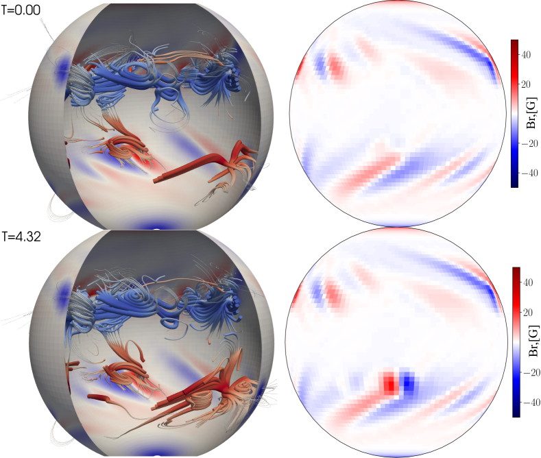
Figure 18: Snapshots of magnetic regions in the south hemisphere in ascending phase of the magnetic cycle. The left column shows the nonaxisymmetric magnetic field lines, time is shown in days. The right column shows the radial magnetic field on the top boundary. Reproduced by permission from Pipin et al (2023).

8.3 Effect of corona on the dynamo

Usually, dynamo models are limited to the star embedded in a vacuum, which is described by boundary conditions on the stellar surface. However, the boundary conditions have a determining influence on the global solutions, such as the symmetry about the equator. With the assumption of an external vacuum, all induction effects in the corona are neglected. Since the solar surface rotates differentially, the highly conductive plasma in the corona also causes induction effects through shear. Observations of coronal rotation are very scarce. There is evidence from extended coronal holes of rigid rotation in latitude (Timothy et al, 1975; Bagashvili et al, 2017). Kinematic dynamo models involving the corona with various assumptions on its rotation and conductivity give a wide range of solutions (Elstner et al, 2020). A notable influence of the corona on the dynamo in the convection zone was also observed in DNS by Warnecke et al (2016). A too weak density contrast and too strong viscous coupling of the corona to the star in their model probably underestimates the effect of the Lorentz force in the corona. Considering a dynamical situation with dominant Lorentz force in the corona, the solution in the Sun corresponds to that with vacuum boundary condition independent of rotation and conductivity in the corona. The magnetic field in the corona varies in time to a nearly force-free solution. Further investigations of the star-corona coupling are needed to clarify the exchange of magnetic energy and helicity.

8.4 Stellar cycle periods

Noyes et al (1984) developed an early understanding of the observed stellar cycle periods, $P_{\rm cyc}$. In those years, there where just six stars with measured rotation and cycle periods. Remarkably, for the stars of Noyes et al (1984), those values have not changed much with the more accurate data of Baliunas et al (1995); see Table 8.4 for a comparison of their cycle periods and the more recent data sets (Olspert et al, 2018; Boro Saikia et al, 2018; Bonanno and Corsaro, 2022). However, for the many stars of Baliunas et al (1995), the modern analysis of Olspert et al (2018) and Boro Saikia et al (2018) showed considerable changes in the results for stellar cycle periodicities. In particular, many of the double periodicities of Baliunas et al (1995) vanished when extended data became available, and different methods were used.

Table 1: Comparison of cycle periods $P_{\rm cyc}$ (in years) from Noyes et al (1984) (NWV84), Baliunas et al (1995) (Bal+95), and Bonanno and Corsaro (2022) (BC22). The last two columns compare the seismic age given by BC22 and the gyrochronological age as listed by Brandenburg et al (2017b) (BMM17). The latter differ significantly, but the determined cycle periods were remarkably stable over the decades.

—— $P_{\rm cyc}$ [yr] ——  — age [Gyr] — HD NWV84 Bal+95 BC22 BC22 BMM17 3651 10 13.8 14.70 — 7.2 4628 8.5 8.37 8.47 3.33 5.3 16160 11.5 13.2 12.68 — 6.9 160346 7 7.00 7.19 — 4.4 201091 7 7.3 7.11 6.10 3.3 201092 11 11.7 — — 3.2

Table 2: Comparison of stellar cycle properties from the samples of Bonanno and Corsaro (2022) and Brandenburg et al (2017b) (indicated as “old”). The blue italics and red roman letters refer to the stars discussed in Brandenburg et al (2017b) and are also indicated in Fig. 19.

HD Sym $\log\langle R_{\rm HK}^{\prime}\rangle$ $\log\langle R_{\rm HK}^{{}^{\prime}\rm old}\rangle$ $P_{\rm rot}$ [d] $P_{\rm rot}^{\rm old}$ [d] $P_{\rm cyc}$ [yr] $P_{\rm cyc}^{\rm I}$ [yr] $P_{\rm cyc}^{\rm A}$ [yr] 100180 h $-4.83$ $-4.92$ 14.06 14.00 3.60 3.60 12.90 103095 i $-4.90$ $-4.90$ 32.51 31.00 7.07 7.30 — 10476 c $-4.97$ $-4.91$ 35.40 35.20 10.45 9.60 — 146233 l $-4.95$ $-4.93$ 22.66 22.70 11.59 7.10 — 160346 m $-4.86$ $-4.79$ 34.20 36.40 7.19 7.00 — 16160 d $-4.94$ $-4.96$ 48.29 48.00 12.68 13.20 — 165341 n $-4.61$ $-4.55$ 19.51 19.00 5.09 5.10 15.50 166620 o $-5.00$ $-4.96$ 42.25 42.40 16.81 15.80 — 219834 s $-4.93$ $-4.94$ 38.89 43.00 9.48 10.00 — 26965 f $-4.96$ $-4.87$ 40.83 43.00 10.24 10.10 — 3651 a $-5.06$ $-4.99$ 40.50 44.00 14.70 13.80 — 4628 b $-4.95$ $-4.85$ 37.82 38.50 8.47 8.60 — 81809 g $-4.89$ $-4.92$ 40.93 40.20 8.05 8.20 — 219834 r $-5.10$ $-5.07$ 43.40 42.00 16.29 21.00 — 201091 p $-4.56$ $-4.76$ 35.62 35.40 7.11 7.30 — Sun a $-4.94$ $-4.90$ 25.55 25.40 10.70 11.00 80.00 149661 K $-4.61$ $-4.58$ 20.92 21.10 12.38 4.00 17.40 152391 M $-4.46$ $-4.45$ 11.01 11.40 11.94 — 10.90 156026 L $-4.56$ $-4.66$ 18.85 21.00 19.31 — 21.00 190406 N $-4.76$ $-4.80$ 14.01 13.90 18.61 2.60 16.90 76151 F $-4.68$ $-4.66$ 14.70 15.00 16.34 2.50 — 78366 G $-4.57$ $-4.61$ 9.60 9.70 14.26 5.90 12.20 114710 J $-4.74$ $-4.75$ 11.99 12.30 14.12 9.60 16.60 22049 E $-4.46$ $-4.46$ 11.09 11.10 11.00 2.90 12.70

In recent work of Bonanno and Corsaro (2022), new cycle data were collected for altogether 67 stars. Their new sample includes stars with less accurate data points, so the existence of different branches was no longer a pronounced feature. In addition, many of the new data points are different from the earlier ones of Brandenburg et al (2017b); see Table 2. As in their paper, we denote G and F dwarfs by the same blue italic symbols and K dwarfs by the same red roman symbols.

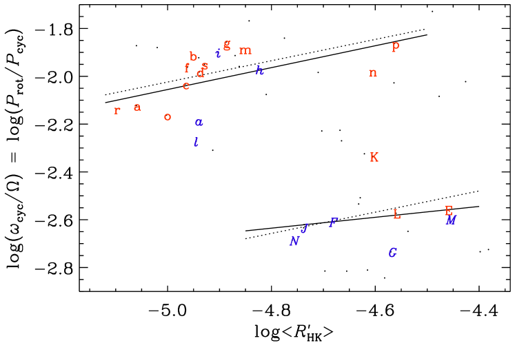
Figure 19: $P_{\rm rot}/P_{\rm cyc}$ versus $\log\langle R_{\rm HK}^{\prime}\rangle$ for all stars of Bonanno and Corsaro (2022) (small black symbols). Lowercase (uppercase) letters denote data points of Bonanno and Corsaro (2022) that were also included in the sample of Brandenburg et al (2017b). There are refer to the data of stars given in the Table 2. The dotted lines denote the fits determined by Brandenburg et al (2017b) while the upper (lower) solid lines denote fits to the stars of Bonanno and Corsaro (2022) with lowercase (uppercase) letters.

To see how strong this revision of the data is, we plot in Fig. 19 the ratios $P_{\rm rot}/P_{\rm cyc}$ versus $\log\langle R_{\rm HK}^{\prime}\rangle$ for all stars of Bonanno and Corsaro (2022) and highlight with lowercase and uppercase letters the stars that were also included in the sample of Brandenburg et al (2017b). We see that the new data are remarkably consistent with the old ones. Out of the eight stars on the branch of active stars, five where listed by Brandenburg et al (2017b) as having two periods. Of the 16 inactive stars, three were listed with two periods, but the case of the Sun was classified by Brandenburg et al (2017b) as somewhat different, because the 80 years Gleissberg cycle does not fit well on the active branch and, unlike all the other stars with two cycle periods, which are all younger than $3.3\,{\rm Gyr}$, the Sun is relatively old.

The early data of Noyes et al (1984) did already suggest

$$\omega_{\rm cyc}\propto\Omega^{1.25}$$ (63)

for the cycle frequency $\omega_{\rm cyc}=2\pi/P_{\rm cyc}$ versus angular rotation rate $\Omega$. This dependence is reproduced by considering free dynamo waves and assuming axisymmetric mean fields, ${\overline{\bm{B}}}=b\hat{\bm{\phi}}+{\bm{\nabla}}\times a\hat{\bm{\phi}}$, with $(a,b)\propto e^{{\rm i}(ky-\omega t)}$ and writing $-{\rm i}\omega=-{\rm i}\omega_{\rm cyc}+\lambda$, where both $\omega_{\rm cyc}$ and $\lambda$ are assumed to be real. The mean-field dynamo equations result in traveling wave solutions with a dispersion relation of the form

$$\omega_{\rm cyc}=\sqrt{\alpha\Omega^{\prime}kL/2},\quad\lambda=\omega_{\rm cyc}-\eta_{\rm T}k^{2}.$$ (64)

At least up to moderate rotation rates, it is reasonable to assume that $\alpha$ and $\Omega^{\prime}$ are proportional to $\Omega$. The crucial assumption in arriving at an approximation that matches Eq. (63) is to assume that the relevant wavenumber $k_{y}$ is selected not by the condition of marginal excitation, but by the assumption that $\lambda=\lambda(k)$ is maximized. Thus, $k$ has to obey ${\rm d}{}\lambda/{\rm d}{}k=0$, which yields $\omega_{\rm cyc}\propto(\alpha\Omega^{\prime})^{2/3}\propto\Omega^{4/3}$. By contrast, if the dynamo is quenched to the being marginally excited, then $\omega_{\rm cyc}\approx\eta_{\rm T}/L^{2}$, which would be either independent of $\Omega$, or perhaps even decreasing with $\Omega$, if $\eta_{\rm T}$ decreases with increasing $\Omega$ due to quenching.

Of course, nonlinear dynamos must always be quenched to reach a steady state. This led Brandenburg et al (1998) to suggest that Eq. (63) could be obeyed if both $\alpha$ and $\eta_{\rm T}$ are antiquenched in such a way that $\eta_{\rm T}$ is antiquenched more slowly than $\alpha$, so that $\omega_{\rm cyc}$ would increase with increasing magnetic field strength, and yet the dynamo would still saturate. Whether this is the only viable solution to this puzzle remains still unclear.

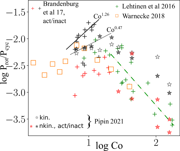
Figure 20: Dependence of cycle period on stellar rotation rate. Red and black crosses show the results of Brandenburg et al (2017b), green crosses those of Lehtinen et al (2016), orange squares the models of Warnecke (2018), and the asterisks are from the models of Pipin (2021); act/inact marks the active and inactive branches of activity, respectively; while kin/nkin stand for kinematic and nonkinematic models, respectively (adapted by permission from Pipin, 2021).

Recently, a number of numerical dynamo models were applied to investigate the relation of the cycle period on the stellar rotation rate in solar analogs (Pipin, 2015; Strugarek et al, 2017; Warnecke, 2018; Viviani et al, 2018; Hazra et al, 2019; Noraz et al, 2022). Figure 20 shows some of these results including the results of observations of Brandenburg et al (2017b) and the survey of Lehtinen et al (2016). It is interesting that the saturation branch of stellar activity for the young solar analogs with rotation periods of less than 10 days is well reproduced in the very different solar-like dynamo models including various GCD simulations (Strugarek et al, 2017; Warnecke, 2018; Viviani et al, 2018), flux transport model of Hazra et al (2019) and mean-field model of Pipin (2021). In Fig.20, this branch is marked by the green line.

The mean cycle period in this branch is almost independent of stellar rotation rate. The nonkinematic nonlinear model of Pipin (2021) shows multiple periods along this line. Pipin (2021) found that saturation of dynamo activity is accompanied by a depression of latitudinal shear, a concentration of magnetic activity to the surface, and changes in the meridional circulations from one cell to multiple cells per hemisphere structure. According to the conclusions of this paper, it is clear that in the saturated state, dynamo waves do not follow the Parker–Yoshimura rule. Their cycle period is determined by turbulent diffusion and meridional circulation. This is why the predictions of flux transport and nonkinematic mean-field dynamo models coincide. The independence of the cycle period on the rotation rate can be typical for the dynamo solutions which show concentration of the magnetic activity toward the boundaries of the dynamo (see Pipin, 2015; Pipin and Kosovichev, 2016).

The inactive branch of the nonkinematic mean-field dynamo models shows a fairly strong positive inclination (see Fig. 20), which is absent in the kinematic models. We see that the dynamo model can reproduce a power law $\sim\mbox{\rm Co}^{0.5}$, avoiding the antiquenching concept of Brandenburg et al (1998). In fact, the nonkinematic dynamo models show a frequency doubling phenomenon for models in the range from 10 to 15 days rotation period (see Figs. 3 and 8 of Pipin, 2021). The frequency doubling or the second harmonic generation is known from nonlinear optics. This is typical for wave propagation in nonlinear media. In dynamo waves, second harmonics are generated because of $\bm{B}^{2}$ effects such as the magnetic feedback on the large-scale flow, magnetic helicity conservation, and magnetic buoyancy effects. The second harmonics can be found in the solar activity as well (Sokoloff et al, 2020). For the solar case, they are subdominant. However, they can become dominant for fast rotating stars. This makes the interpretation of magnetic activity cycles difficult (Stepanov et al, 2020).

It is important to note that the GCD simulations of Viviani et al (2018) show an increased level of nonaxisymmetry with an increase of rotation rate and a transition to preferred nonaxisymmetric dynamos for solar-type stars with a rotation period of less than 14 days. In simulations, this transition happens when the rotation profile changes from an antisolar to a solar-like profile with a faster equator and slow poles. Stellar Zeeman Doppler Imaging observations of Donati and Landstreet (2009) and See et al (2016), for example, show that the magnetic topology depends on stellar mass and rotation rate. In a certain interval of rotation periods (below $14\,{\rm d}$) and stellar mass, the results of Viviani et al (2018) are compatible with the observational findings mentioned above.

Summarizing, we suggest that the Parker–Yoshimura dynamo regime can work for solar analogs rotating with periods above 14–15 days. In an interval of stellar rotation periods between 10 and 15 days, frequency doubling and a transition to the nonaxisymmetric dynamos occurs. For lower rotation periods, the dynamo transits to a saturation stage. It can be characterized by high magnetic activity and multiple dynamo periods which are independent of stellar rotation rate. This new picture should be further improved by including possible dynamo effects of surface activity in the form of bipolar magnetic regions and star spots.

Another interesting observation is that different types of stars, including partially convective main sequence solar-type stars, fully convective M-dwarfs, and evolved post-main sequence giant stars show similar scaling with the Rossby number for the unsaturated regime (see, e.g., Wright and Drake, 2016; Wright et al, 2018; Lehtinen et al, 2020). In particular, to derive the Rossby number, these study employ a simple parameterization of the convective turnover time suggested by stellar interior models. It was found that for evolved stars, the Rossby-independent parameterizations break down in the rotation–activity relation (Lehtinen et al, 2020). This constitutes a strong argument in favor of the turbulent dynamo paradigm suggesting a common role of the turbulent process in dynamos operating in these stars.

8.5 Analogy of mean-field $\alpha$ and the chiral magnetic effect

The $\alpha$ effect in mean-field dynamo theory is an effect that emerges after averaging over the scale of several turbulent eddies. We know already that turbulent diffusion is somewhat analogous to microphysical diffusion, which also emerges after averaging, but here after averaging over atomic scales. Interestingly, even for the $\alpha$ effect there can be an effect on atomic and subatomic scales, because fermions, such as electrons, are chiral. The spin of an electron emerging from the decay of a neutron is anti-aligned with its momentum vector, so their dot product is a negative pseudo-scalar, called the chirality. Positrons have positive chirality. In the presence of an ambient magnetic field, the spins align, but electrons and positrons move in opposite directions, causing therefore an electric current. This constitutes a microscopic $\alpha$ effect (Rogachevskii et al, 2017; Brandenburg et al, 2017c),

$$\alpha_{\rm micro}\equiv\mu_{5}\eta=24\alpha_{\rm fine}(n_{\rm L}-n_{\rm R})(\hbar c/k_{\rm B}T)^{2},$$ (65)

where $\mu_{5}$ is the normalized chiral chemical potential (with units of inverse length), $\eta$ is the microscopic magnetic diffusivity, $\alpha_{\rm fine}\approx 1/137$ is the fine structure constant (quantifying the strength of electromagnetic interaction between charged particles), $n_{\rm L}$ and $n_{\rm R}$ are the number densities of left- and right-handed fermions, $\hbar\approx 10^{-27}\,{\rm erg}\,{\rm s}$ is the reduced Planck constant, $c\approx 3\times 10^{10}\,{\rm cm}\,{\rm s}^{-1}$ is the speed of light, $k_{\rm B}\approx 10^{-16}\,{\rm erg}\,{\rm K}^{-1}$ is the Boltzmann constant, and $T$ is the temperature.

The applications of chiral MHD are manifold and range from condensed matter systems and heavy ion collisions to neutron stars and the early Universe; see Kharzeev (2014) for a review. Interestingly, because this microscopic $\alpha$ effect produces helical magnetic fields, and because the total chirality is conserved (Boyarsky et al, 2012), this effect does not last forever, but is being quenched in a form analogous to the catastrophic quenching formula, which takes the form (Rogachevskii et al, 2017)

$$\frac{\partial\mu_{5}}{\partial t}=-\lambda\eta\left(\mu_{5}{\overline{\bm{B}}}^{2}-\eta_{\rm t}\mu_{0}{\overline{\bm{J}}}\cdot{\overline{\bm{B}}}\right)-\Gamma_{\rm flip}\mu_{5},$$ (66)

where $\lambda$ is a coupling constant which, in the catastrophic quenching formalism, is related to $2\eta_{\rm t}k_{\rm f}^{2}/B_{\rm eq}^{2}$, and $\Gamma_{\rm flip}$ is a spin-flipping parameter, which is related to $2\eta k_{\rm f}^{2}$ in the catastrophic quenching formalism (see, e.g., Field and Blackman, 2002; Blackman and Brandenburg, 2002).

There is a vast range of recent work in this field, which goes well beyond the scope of the present paper. We just mention here the paper of Masada et al (2018), who studied chiral magnetohydrodynamic turbulence in core-collapse supernovae. They found that the inverse cascade related to the chiral effects impacts the magnetohydrodynamic evolution in the supernova core toward explosion.

8.6 Direct Statistical Simulations

An alternative or extension to mean-field theory in the usual sense is to solve the time-dependent system of one-point and two-point correlation functions. This is what is now known as Direct Statistical Simulations (Tobias et al, 2011; Tobias and Marston, 2013, 2017) and has primarily been applied to two-dimensional turbulent shear flow problems. The dimensionality of the two-point correlation function doubles for those directions over which homogeneity cannot be assumed. On the other hand, the dynamics of the low order statistics is usually slower than that of the original equations. In addition, it is possible to reduce the complexity of the problem by employing Proper Orthogonal Decomposition (Allawala and Marston, 2016; Allawala et al, 2020). This approach has not yet been applied to magnetohydrodynamics and the dynamo problem. Such an approach would be able to incorporate both small-scale and large-scale dynamos at the same time. The small-scale dynamo problem would be solved through correlation functions, as has been done in Brandenburg and Subramanian (2000), for example. But their simulations were isotropic and did not include anisotropic dependencies on position. Nevertheless, this approach has the potential of being a strong competitor in addressing the high Reynolds number dynamics of problems of astrophysical and geophysical relevance; see Tobias (2021) for a recent review touching on these aspects.

9 Looking forward

In this review, we have provided some insight into recent developments in our understanding of the generation of astrophysical large-scale magnetic fields. The current development of mean-field theory allows us to go beyond some of the original restrictions that were related to the assumption of large scale-separation and the inappropriate neglect of nonlinear effects due to higher order correlations in contributions to the mean turbulent electromotive force. A big portion of the progress comes from the development in the DNS of astrophysical turbulence. Noteworthy, the classical mean-field theory is based on the fundamental equations of electrodynamics and has well-known limits. With the new steps forward, we can take into account results of the DNS, e.g., the spectral kernels, and treat them as experimental facts. The necessity of some phenomenological additions to classical mean-field theory are motivated both by DNS and observations of the magnetic activity in astrophysical systems, such as those in our Sun and other stars. In this way, mean-field models become a valuable tool to understand the real and virtual worlds of the dynamo in stars and in DNS.

Declarations

Competing Interests  The authors declare they have no conflicts of interest.

Open Access  This article is licensed under a Creative Commons Attribution 4.0 International License, which permits use, sharing, adaptation, distribution and reproduction in any medium or format, as long as you give appropriate credit to the original author(s) and the source, provide a link to the Creative Commons licence, and indicate if changes were made. The images or other third party material in this article are included in the article’s Creative Commons licence, unless indicated otherwise in a credit line to the material. If material is not included in the article’s Creative Commons licence and your intended use is not permitted by statutory regulation or exceeds the permitted use, you will need to obtain permission directly from the copyright holder. To view a copy of this licence, visit http://creativecommons.org/licenses/by/4.0/.

References

- Allawala and Marston (2016) Allawala A, Marston JB (2016) Statistics of the stochastically forced Lorenz attractor by the Fokker-Planck equation and cumulant expansions. PhRvE 94(5):052218, DOI 10.1103/PhysRevE.94.052218, 1604.00867
- Allawala et al (2020) Allawala A, Tobias SM, Marston JB (2020) Dimensional reduction of direct statistical simulation. J Fluid Mech 898:A21, DOI 10.1017/jfm.2020.382, 1708.07805
- Altrock et al (2008) Altrock R, Howe R, Ulrich R (2008) Solar torsional oscillations and their relationship to coronal activity. In: Howe R, Komm RW, Balasubramaniam KS, Petrie GJD (eds) Subsurface and Atmospheric Influences on Solar Activity, Astron. Soc. Pacif. Conf. Ser., vol 383, p 335
- Augustson et al (2015) Augustson K, Brun AS, Miesch M, Toomre J (2015) Grand Minima and Equatorward Propagation in a Cycling Stellar Convective Dynamo. ApJ 809(2):149, DOI 10.1088/0004-637X/809/2/149, 1410.6547
- Bagashvili et al (2017) Bagashvili SR, Shergelashvili BM, Japaridze DR, Chargeishvili BB, Kosovichev AG, Kukhianidze V, Ramishvili G, Zaqarashvili TV, Poedts S, Khodachenko ML, De Causmaecker P (2017) Statistical properties of coronal hole rotation rates: Are they linked to the solar interior? A&A 603:A134, DOI 10.1051/0004-6361/201630377, 1706.04464
- Baliunas et al (1995) Baliunas SL, Donahue RA, Soon WH, Horne JH, Frazer J, Woodard-Eklund L, Bradford M, Rao LM, Wilson OC, Zhang Q, Bennett W, Briggs J, Carroll SM, Duncan DK, Figueroa D, Lanning HH, Misch T, Mueller J, Noyes RW, Poppe D, Porter AC, Robinson CR, Russell J, Shelton JC, Soyumer T, Vaughan AH, Whitney JH (1995) Chromospheric variations in main-sequence stars. ApJ 438:269–287, DOI 10.1086/175072
- Baryshnikova and Shukurov (1987) Baryshnikova I, Shukurov A (1987) Oscillatory alpha-squared dynamo - Numerical investigation. Astronomische Nachrichten 308(2):89–100, DOI 10.1002/asna.2113080202
- Beaudoin et al (2013) Beaudoin P, Charbonneau P, Racine E, Smolarkiewicz PK (2013) Torsional oscillations in a global solar dynamo. Sol. Phys. 282(2):335–360, DOI 10.1007/s11207-012-0150-2, 1210.1209
- Berdyugina (2005) Berdyugina SV (2005) Starspots: A Key to the Stellar Dynamo. Living Reviews in Solar Physics 2(1):8, DOI 10.12942/lrsp-2005-8
- Biskamp and Müller (1999) Biskamp D, Müller WC (1999) Decay Laws for Three-Dimensional Magnetohydrodynamic Turbulence. PhRvL 83(11):2195–2198, DOI 10.1103/PhysRevLett.83.2195, physics/9903028
- Blackman and Brandenburg (2002) Blackman EG, Brandenburg A (2002) Dynamic Nonlinearity in Large-Scale Dynamos with Shear. ApJ 579(1):359–373, DOI 10.1086/342705, astro-ph/0204497
- Blackman and Ji (2006) Blackman EG, Ji H (2006) Laboratory plasma dynamos, astrophysical dynamos and magnetic helicity evolution. MNRAS 369(4):1837–1848, DOI 10.1111/j.1365-2966.2006.10431.x, astro-ph/0604221
- Bonanno and Corsaro (2022) Bonanno A, Corsaro E (2022) On the Origin of the Dichotomy of Stellar Activity Cycles. ApJL 939(2):L26, DOI 10.3847/2041-8213/ac9c05, 2210.11305
- Boro Saikia et al (2018) Boro Saikia S, Marvin CJ, Jeffers SV, Reiners A, Cameron R, Marsden SC, Petit P, Warnecke J, Yadav AP (2018) Chromospheric activity catalogue of 4454 cool stars. Questioning the active branch of stellar activity cycles. A&A 616:A108, DOI 10.1051/0004-6361/201629518, 1803.11123
- Boyarsky et al (2012) Boyarsky A, Fröhlich J, Ruchayskiy O (2012) Self-Consistent Evolution of Magnetic Fields and Chiral Asymmetry in the Early Universe. PhRvL 108(3):031301, DOI 10.1103/PhysRevLett.108.031301, 1109.3350
- Brandenburg (1998) Brandenburg A (1998) Disc turbulence and viscosity. In: Abramowicz MA, Björnsson G, Pringle JE (eds) Theory of Black Hole Accretion Disks, pp 61–90
- Brandenburg (2001) Brandenburg A (2001) The Inverse Cascade and Nonlinear Alpha-Effect in Simulations of Isotropic Helical Hydromagnetic Turbulence. ApJ 550(2):824–840, DOI 10.1086/319783, astro-ph/0006186
- Brandenburg (2008) Brandenburg A (2008) The dual role of shear in large-scale dynamos. Astron Nachr 329(7):725, DOI 10.1002/asna.200811027, 0808.0959
- Brandenburg (2016) Brandenburg A (2016) Stellar Mixing Length Theory with Entropy Rain. ApJ 832(1):6, DOI 10.3847/0004-637X/832/1/6, 1504.03189
- Brandenburg (2017) Brandenburg A (2017) Analytic solution of an oscillatory migratory 2 stellar dynamo. A&A 598:A117, DOI 10.1051/0004-6361/201630033, 1611.02671
- Brandenburg (2018a) Brandenburg A (2018a) Advances in mean-field dynamo theory and applications to astrophysical turbulence. J Plasma Phys 84(4):735840404, DOI 10.1017/S0022377818000806, 1801.05384
- Brandenburg (2018b) Brandenburg A (2018b) Magnetic helicity and fluxes in an inhomogeneous 2 dynamo. Astron Nachr 339(631):631–640, DOI 10.1002/asna.201913604
- Brandenburg and Chatterjee (2018) Brandenburg A, Chatterjee P (2018) Strong nonlocality variations in a spherical mean-field dynamo. Astron Nachr 339:118–126, DOI 10.1002/asna.201813472, 1802.04231
- Brandenburg and Chen (2020) Brandenburg A, Chen L (2020) The nature of mean-field generation in three classes of optimal dynamos. J Plasma Phys 86(1):905860110, DOI 10.1017/S0022377820000082, 1911.01712
- Brandenburg and Dobler (2001) Brandenburg A, Dobler W (2001) Large scale dynamos with helicity loss through boundaries. A&A 369:329–338, DOI 10.1051/0004-6361:20010123, astro-ph/0012472
- Brandenburg and Hubbard (2015) Brandenburg A, Hubbard PJ A Käpylä (2015) Dynamical quenching with non-local and downward pumping. Astronomische Nachrichten 336(1):91–96, DOI 10.1002/asna.201412141, 1412.0997
- Brandenburg and Käpylä (2007) Brandenburg A, Käpylä PJ (2007) Magnetic helicity effects in astrophysical and laboratory dynamos. New J Phys 9(8):305, DOI 10.1088/1367-2630/9/8/305, 0705.3507
- Brandenburg and Larsson (2023) Brandenburg A, Larsson G (2023) Turbulence with Magnetic Helicity That Is Absent on Average. Atmosphere 14(6):932, DOI 10.3390/atmos14060932, 2305.08769
- Brandenburg and Ntormousi (2023) Brandenburg A, Ntormousi E (2023) Galactic Dynamos. Ann Rev Astron Astrophys 61(1):561–606, DOI 10.1146/annurev-astro-071221-052807, URL https://doi.org/10.1146/annurev-astro-071221-052807
- Brandenburg and Rädler (2013) Brandenburg A, Rädler KH (2013) Yoshizawa’s cross-helicity effect and its quenching. Geophysical and Astrophysical Fluid Dynamics 107(1-2):207–217, DOI 10.1080/03091929.2012.681307, 1112.1237
- Brandenburg and Sokoloff (2002) Brandenburg A, Sokoloff D (2002) Local and Nonlocal Magnetic Diffusion and Alpha-Effect Tensors in Shear Flow Turbulence. Geophysical and Astrophysical Fluid Dynamics 96(4):319–344, DOI 10.1080/03091920290032974, astro-ph/0111568
- Brandenburg and Subramanian (2000) Brandenburg A, Subramanian K (2000) Large scale dynamos with ambipolar diffusion nonlinearity. A&A 361:L33–L36, DOI 10.48550/arXiv.astro-ph/0007450, astro-ph/0007450
- Brandenburg and Subramanian (2005a) Brandenburg A, Subramanian K (2005a) Astrophysical magnetic fields and nonlinear dynamo theory. Phys. Rep. 417:1–209, DOI 10.1016/j.physrep.2005.06.005, arXiv:astro-ph/0405052
- Brandenburg and Subramanian (2005b) Brandenburg A, Subramanian K (2005b) Minimal tau approximation and simulations of the alpha effect. A&A 439(3):835–843, DOI 10.1051/0004-6361:20053221, astro-ph/0504222
- Brandenburg and Subramanian (2005c) Brandenburg A, Subramanian K (2005c) Strong mean field dynamos require supercritical helicity fluxes. Astron Nachr 326:400–408, DOI 10.1002/asna.200510362, astro-ph/0505457
- Brandenburg and Subramanian (2007) Brandenburg A, Subramanian K (2007) Simulations of the anisotropic kinetic and magnetic alpha effects. Astronomische Nachrichten 328(6):507, DOI 10.1002/asna.200710772, 0705.3508
- Brandenburg and Tuominen (1988) Brandenburg A, Tuominen I (1988) Variation of magnetic fields and flows during the solar cycle. Adv Spa Res 8(7):185–189, DOI 10.1016/0273-1177(88)90190-1
- Brandenburg et al (1990) Brandenburg A, Tuominen I, Nordlund A, Pulkkinen P, Stein RF (1990) 3-D simulation of turbulent cyclonic magneto-convection. A&A 232:277–291
- Brandenburg et al (1992) Brandenburg A, Moss D, Tuominen I (1992) Stratification and thermodynamics in mean-field dynamos. A&A 265:328–344
- Brandenburg et al (1996) Brandenburg A, Jennings RL, Nordlund Å, Rieutord M, Stein RF, Tuominen I (1996) Magnetic structures in a dynamo simulation. J Fluid Mech 306:325–352, DOI 10.1017/S0022112096001322
- Brandenburg et al (1998) Brandenburg A, Saar SH, Turpin CR (1998) Time Evolution of the Magnetic Activity Cycle Period. ApJL 498(1):L51–L54, DOI 10.1086/311297
- Brandenburg et al (2008) Brandenburg A, Rädler KH, Schrinner M (2008) Scale dependence of alpha effect and turbulent diffusivity. A&A 482(3):739–746, DOI 10.1051/0004-6361:200809365, 0801.1320
- Brandenburg et al (2009) Brandenburg A, Candelaresi S, Chatterjee P (2009) Small-scale magnetic helicity losses from a mean-field dynamo. MNRAS 398(3):1414–1422, DOI 10.1111/j.1365-2966.2009.15188.x, 0905.0242
- Brandenburg et al (2010) Brandenburg A, Kleeorin N, Rogachevskii I (2010) Large-scale magnetic flux concentrations from turbulent stresses. Astron Nachr 331(1):5, DOI 10.1002/asna.200911311, 0910.1835
- Brandenburg et al (2011) Brandenburg A, Kemel K, Kleeorin N, Mitra D, Rogachevskii I (2011) Detection of Negative Effective Magnetic Pressure Instability in Turbulence Simulations. ApJL 740(2):L50, DOI 10.1088/2041-8205/740/2/L50, 1109.1270
- Brandenburg et al (2012) Brandenburg A, Rädler KH, Kemel K (2012) Mean-field transport in stratified and/or rotating turbulence. A&A 539:A35, DOI 10.1051/0004-6361/201117871, 1108.2264
- Brandenburg et al (2013) Brandenburg A, Kleeorin N, Rogachevskii I (2013) Self-assembly of Shallow Magnetic Spots through Strongly Stratified Turbulence. ApJL 776(2):L23, DOI 10.1088/2041-8205/776/2/L23, 1306.4915
- Brandenburg et al (2014) Brandenburg A, Gressel O, Jabbari S, Kleeorin N, Rogachevskii I (2014) Mean-field and direct numerical simulations of magnetic flux concentrations from vertical field. A&A 562:A53, DOI 10.1051/0004-6361/201322681, 1309.3547
- Brandenburg et al (2017a) Brandenburg A, Ashurova MB, Jabbari S (2017a) Compensating Faraday Depolarization by Magnetic Helicity in the Solar Corona. ApJL 845(2):L15, DOI 10.3847/2041-8213/aa844b, 1706.09540
- Brandenburg et al (2017b) Brandenburg A, Mathur S, Metcalfe TS (2017b) Evolution of Co-existing Long and Short Period Stellar Activity Cycles. ApJ 845(1):79, DOI 10.3847/1538-4357/aa7cfa, 1704.09009
- Brandenburg et al (2017c) Brandenburg A, Schober J, Rogachevskii I, Kahniashvili T, Boyarsky A, Fröhlich J, Ruchayskiy O, Kleeorin N (2017c) The Turbulent Chiral Magnetic Cascade in the Early Universe. ApJL 845(2):L21, DOI 10.3847/2041-8213/aa855d, 1707.03385
- Browning et al (2006) Browning MK, Miesch MS, Brun AS, Toomre J (2006) Dynamo Action in the Solar Convection Zone and Tachocline: Pumping and Organization of Toroidal Fields. ApJL 648(2):L157–L160, DOI 10.1086/507869, astro-ph/0609153
- Brummell et al (1998) Brummell NH, Hurlburt NE, Toomre J (1998) Turbulent Compressible Convection with Rotation. II. Mean Flows and Differential Rotation. ApJ 493(2):955–969, DOI 10.1086/305137
- Brummell et al (2002) Brummell NH, Clune TL, Toomre J (2002) Penetration and Overshooting in Turbulent Compressible Convection. ApJ 570(2):825–854, DOI 10.1086/339626
- Bushby and Tobias (2007) Bushby PJ, Tobias SM (2007) On predicting the solar cycle using mean-field models. ApJ 661:1289–1296, DOI 10.1086/516628, 0704.2345
- Bushby et al (2018) Bushby PJ, Käpylä PJ, Masada Y, Brandenburg A, Favier B, Guervilly C, Käpylä MJ (2018) Large-scale dynamos in rapidly rotating plane layer convection. A&A 612:A97, DOI 10.1051/0004-6361/201732066, 1710.03174
- Cameron and Schüssler (2015) Cameron R, Schüssler M (2015) The crucial role of surface magnetic fields for the solar dynamo. Science 347(6228):1333–1335, DOI 10.1126/science.1261470, 1503.08469
- Candelaresi and Brandenburg (2013) Candelaresi S, Brandenburg A (2013) Kinetic helicity needed to drive large-scale dynamos. PhRvE 87:043104, DOI 10.1103/PhysRevE.87.043104, 1208.4529
- Cattaneo and Hughes (2006) Cattaneo F, Hughes DW (2006) Dynamo action in a rotating convective layer. J Fluid Mech 553:401–418, DOI 10.1017/S0022112006009165
- Chabrier and Küker (2006) Chabrier G, Küker M (2006) Large-scale 2̂-dynamo in low-mass stars and brown dwarfs. A&A 446(3):1027–1037, DOI 10.1051/0004-6361:20042475, astro-ph/0510075
- Charbonneau (2014) Charbonneau P (2014) Solar Dynamo Theory. ARA&A 52:251–290, DOI 10.1146/annurev-astro-081913-040012
- Charbonneau (2020) Charbonneau P (2020) Dynamo Models of the Solar Cycle. Living Reviews in Solar Physics 17(1):3, DOI 10.1007/s41116-020-00025-6
- Chatterjee et al (2010) Chatterjee P, Brandenburg A, Guerrero G (2010) Can catastrophic quenching be alleviated by separating shear and effect? Geophysical and Astrophysical Fluid Dynamics 104(5):591–599, DOI 10.1080/03091929.2010.504185, 1005.5708
- Chatterjee et al (2011) Chatterjee P, Guerrero G, Brandenburg A (2011) Magnetic helicity fluxes in interface and flux transport dynamos. A&A 525:A5, DOI 10.1051/0004-6361/201015073, 1005.5335
- Choudhuri et al (2007) Choudhuri AR, Chatterjee P, Jiang J (2007) Predicting solar cycle 24 with a solar dynamo model. Phys Rev Lett 98(13):131103, DOI 10.1103/PhysRevLett.98.131103, arXiv:astro-ph/0701527
- Covas et al (2000) Covas E, Tavakol R, Moss D, Tworkowski A (2000) Torsional oscillations in the solar convection zone. A&A 360:L21–L24, astro-ph/0010323
- Cowling (1933) Cowling TG (1933) The magnetic field of sunspots. MNRAS 94:39–48, DOI 10.1093/mnras/94.1.39
- Davidson (2000) Davidson PA (2000) Was Loitsyansky correct? A review of the arguments. J Turbulence 1(1):6, DOI 10.1088/1468-5248/1/1/006
- Deardorff (1972) Deardorff JW (1972) Theoretical expression for the countergradient vertical heat flux. J Geophys Res 77(30):5900–5904, DOI 10.1029/JC077i030p05900
- Del Sordo et al (2013) Del Sordo F, Guerrero G, Brandenburg A (2013) Turbulent dynamos with advective magnetic helicity flux. MNRAS 429(2):1686–1694, DOI 10.1093/mnras/sts398, 1205.3502
- Donati and Landstreet (2009) Donati JF, Landstreet JD (2009) Magnetic fields of nondegenerate stars. ARA&A 47:333–370, DOI 10.1146/annurev-astro-082708-101833, 0904.1938
- Egorov et al (2004) Egorov P, Rüdiger G, Ziegler U (2004) Vorticity and helicity of the solar supergranulation flow-field. A&A 425:725–728, DOI 10.1051/0004-6361:20040531
- Elstner and Rüdiger (2007) Elstner D, Rüdiger G (2007) How can 2-dynamos generate axisymmetric magnetic fields? Astron Nachr 328(10):1130–1132, DOI 10.1002/asna.200710864
- Elstner et al (2020) Elstner D, Fournier Y, Arlt R (2020) Various scenarios for the equatorward migration of sunspots. In: Kosovichev A, Strassmeier S, Jardine M (eds) Solar and Stellar Magnetic Fields: Origins and Manifestations, vol 354, pp 134–137, DOI 10.1017/S1743921319009888, 2003.08131
- Fan and Fang (2014) Fan Y, Fang F (2014) A Simulation of Convective Dynamo in the Solar Convective Envelope: Maintenance of the Solar-like Differential Rotation and Emerging Flux. ApJ 789(1):35, DOI 10.1088/0004-637X/789/1/35, %****␣paper.bbl␣Line␣425␣****1405.3926
- Favier and Bushby (2013) Favier B, Bushby PJ (2013) On the problem of large-scale magnetic field generation in rotating compressible convection. J Fluid Mech 723:529–555, DOI 10.1017/jfm.2013.132, 1302.7243
- Ferriere (1993) Ferriere K (1993) The Full Alpha-Tensor Due to Supernova Explosions and Superbubbles in the Galactic Disk. ApJ 404:162, DOI 10.1086/172266
- Field and Blackman (2002) Field GB, Blackman EG (2002) Dynamical Quenching of the 2 Dynamo. ApJ 572(1):685–692, DOI 10.1086/340233, astro-ph/0111470
- Getling et al (2021) Getling AV, Kosovichev AG, Zhao J (2021) Evolution of Subsurface Zonal and Meridional Flows in Solar Cycle 24 from Helioseismological Data. ApJL 908(2):L50, DOI 10.3847/2041-8213/abe45a, 2012.15555
- Ghizaru et al (2010) Ghizaru M, Charbonneau P, Smolarkiewicz PK (2010) Magnetic Cycles in Global Large-eddy Simulations of Solar Convection. ApJL 715(2):L133–L137, DOI 10.1088/2041-8205/715/2/L133
- Gopalakrishnan and Subramanian (2023) Gopalakrishnan K, Subramanian K (2023) Magnetic Helicity Fluxes from Triple Correlators. ApJ 943(1):66, DOI 10.3847/1538-4357/aca808, 2209.14810
- Gressel (2010) Gressel O (2010) A mean-field approach to the propagation of field patterns in stratified magnetorotational turbulence. MNRAS 405(1):41–48, DOI 10.1111/j.1365-2966.2010.16440.x, 1001.5250
- Gruzinov and Diamond (1994) Gruzinov AV, Diamond PH (1994) Self-consistent theory of mean-field electrodynamics. PhRvL 72(11):1651–1653, DOI 10.1103/PhysRevLett.72.1651
- Guerrero et al (2016) Guerrero G, Smolarkiewicz PK, de Gouveia Dal Pino EM, Kosovichev AG, Mansour NN (2016) Understanding solar torsional oscillations from global dynamo models. ApJL 828:L3, DOI 10.3847/2041-8205/828/1/L3, 1608.02278
- Hanasoge et al (2016) Hanasoge S, Gizon L, Sreenivasan KR (2016) Seismic Sounding of Convection in the Sun. Annual Review of Fluid Mechanics 48(1):191–217, DOI 10.1146/annurev-fluid-122414-034534, 1503.07961
- Hathaway (2012) Hathaway DH (2012) Supergranules as probes of the sun’s meridional circulation. ApJ 760:84, DOI 10.1088/0004-637X/760/1/84, 1210.3343
- Hathaway (2015) Hathaway DH (2015) The Solar Cycle. Living Reviews in Solar Physics 12(1):4, DOI 10.1007/lrsp-2015-4, 1502.07020
- Hatori (1984) Hatori T (1984) Kolmogorov-Style Argument for the Decaying Homogeneous MHD Turbulence. J Phys Soc Jpn 53(8):2539, DOI 10.1143/JPSJ.53.2539
- Hazra and Choudhuri (2017) Hazra G, Choudhuri AR (2017) A theoretical model of the variation of the meridional circulation with the solar cycle. MNRAS 472(3):2728–2741, DOI 10.1093/mnras/stx2152, 1708.05204
- Hazra et al (2019) Hazra G, Jiang J, Karak BB, Kitchatinov L (2019) Exploring the Cycle Period and Parity of Stellar Magnetic Activity with Dynamo Modeling. ApJ 884(1):35, DOI 10.3847/1538-4357/ab4128, 1909.01286
- Hazra et al (2023) Hazra G, Nandy D, Kitchatinov L, Choudhuri AR (2023) Mean Field Models of Flux Transport Dynamo and Meridional Circulation in the Sun and Stars. Space. Sci. Rev. 219(5):39, DOI 10.1007/s11214-023-00982-y, 2302.09390
- Hotta and Kusano (2021) Hotta H, Kusano K (2021) Solar differential rotation reproduced with high-resolution simulation. Nature Astronomy 5:1100–1102, DOI 10.1038/s41550-021-01459-0, 2109.06280
- Hotta et al (2016) Hotta H, Rempel M, Yokoyama T (2016) Large-scale magnetic fields at high Reynolds numbers in magnetohydrodynamic simulations. Science 351(6280):1427–1430, DOI 10.1126/science.aad1893
- Howard and Labonte (1980) Howard R, Labonte BJ (1980) The sun is observed to be a torsional oscillator with a period of 11 years. ApJL 239:L33–L36, DOI 10.1086/183286
- Howe et al (2011) Howe R, Hill F, Komm R, Christensen-Dalsgaard J, Larson TP, Schou J, Thompson MJ, Ulrich R (2011) The torsional oscillation and the new solar cycle. J Phys Conf Ser 271(1):012074, DOI 10.1088/1742-6596/271/1/012074
- Hubbard and Brandenburg (2009) Hubbard A, Brandenburg A (2009) Memory Effects in Turbulent Transport. ApJ 706(1):712–726, DOI 10.1088/0004-637X/706/1/712, 0811.2561
- Hubbard and Brandenburg (2012) Hubbard A, Brandenburg A (2012) Catastrophic quenching in dynamos revisited. ApJ 748:51, DOI 10.1088/0004-637X/748/1/51, 1107.0238
- Hubbard et al (2009) Hubbard A, Del Sordo F, Käpylä PJ, Brandenburg A (2009) The effect with imposed and dynamo-generated magnetic fields. MNRAS 398(4):1891–1899, DOI 10.1111/j.1365-2966.2009.15108.x, 0904.2773
- Jabbari et al (2014) Jabbari S, Brandenburg A, Losada IR, Kleeorin N, Rogachevskii I (2014) Magnetic flux concentrations from dynamo-generated fields. A&A 568:A112, DOI 10.1051/0004-6361/201423499, 1401.6107
- Jabbari et al (2016) Jabbari S, Brandenburg A, Mitra D, Kleeorin N, Rogachevskii I (2016) Turbulent reconnection of magnetic bipoles in stratified turbulence. MNRAS 459(4):4046–4056, DOI 10.1093/mnras/stw888, 1601.08167
- Ji (1999) Ji H (1999) Turbulent Dynamos and Magnetic Helicity. PhRvL 83(16):3198–3201, DOI 10.1103/PhysRevLett.83.3198, astro-ph/0102321
- Ji and Prager (2002) Ji H, Prager SC (2002) The dynamo effects in laboratory plasmas. Magnetohydrodynamics 38:191–210, DOI 10.22364/mhd.38.1-2.15, astro-ph/0110352
- Ji et al (1995) Ji H, Prager SC, Sarff JS (1995) Conservation of Magnetic Helicity during Plasma Relaxation. PhRvL 74(15):2945–2948, DOI 10.1103/PhysRevLett.74.2945
- Kaneda et al (2003) Kaneda Y, Ishihara T, Yokokawa M, Itakura K, Uno A (2003) Energy dissipation rate and energy spectrum in high resolution direct numerical simulations of turbulence in a periodic box. Physics of Fluids 15(2):L21–L24, DOI 10.1063/1.1539855
- Käpylä et al (2016a) Käpylä MJ, Käpylä PJ, Olspert N, Brandenburg A, Warnecke J, Karak BB, Pelt J (2016a) Multiple dynamo modes as a mechanism for long-term solar activity variations. A&A 589:A56, DOI 10.1051/0004-6361/201527002, 1507.05417
- Käpylä et al (2022) Käpylä MJ, Rheinhardt M, Brandenburg A (2022) Compressible Test-field Method and Its Application to Shear Dynamos. ApJ 932(1):8, DOI 10.3847/1538-4357/ac5b78, 2106.01107
- Käpylä et al (2004) Käpylä PJ, Korpi MJ, Tuominen I (2004) Local models of stellar convection:. Reynolds stresses and turbulent heat transport. A&A 422:793–816, DOI 10.1051/0004-6361:20035874, astro-ph/0312376
- Käpylä et al (2006a) Käpylä PJ, Korpi MJ, Ossendrijver M, Stix M (2006a) Magnetoconvection and dynamo coefficients. III. -effect and magnetic pumping in the rapid rotation regime. A&A 455(2):401–412, DOI 10.1051/0004-6361:20064972, astro-ph/0602111
- Käpylä et al (2006b) Käpylä PJ, Korpi MJ, Tuominen I (2006b) Solar dynamo models with -effect and turbulent pumping from local 3D convection calculations. Astronomische Nachrichten 327(9):884, DOI 10.1002/asna.200610636, astro-ph/0606089
- Käpylä et al (2009a) Käpylä PJ, Korpi MJ, Brandenburg A (2009a) Alpha effect and turbulent diffusion from convection. A&A 500(2):633–646, DOI 10.1051/0004-6361/200811498, 0812.1792
- Käpylä et al (2009b) Käpylä PJ, Korpi MJ, Brandenburg A (2009b) Large-scale Dynamos in Rigidly Rotating Turbulent Convection. ApJ 697(2):1153–1163, DOI 10.1088/0004-637X/697/2/1153, 0812.3958
- Käpylä et al (2012) Käpylä PJ, Mantere MJ, Brandenburg A (2012) Cyclic Magnetic Activity due to Turbulent Convection in Spherical Wedge Geometry. ApJL 755(1):L22, DOI 10.1088/2041-8205/755/1/L22, 1205.4719
- Käpylä et al (2013) Käpylä PJ, Mantere MJ, Brandenburg A (2013) Oscillatory large-scale dynamos from Cartesian convection simulations. Geophysical and Astrophysical Fluid Dynamics 107(1-2):244–257, DOI 10.1080/03091929.2012.715158, 1111.6894
- Käpylä et al (2016b) Käpylä PJ, Brandenburg A, Kleeorin N, Käpylä MJ, Rogachevskii I (2016b) Magnetic flux concentrations from turbulent stratified convection. A&A 588:A150, DOI 10.1051/0004-6361/201527731, 1511.03718
- Käpylä et al (2023) Käpylä PJ, Browning MK, Brun AS, Guerrero G, Warnecke J (2023) Simulations of solar and stellar dynamos and their theoretical interpretation. arXiv e-prints arXiv:2305.16790, DOI 10.48550/arXiv.2305.16790, 2305.16790
- Karak (2023) Karak BB (2023) Models for the long-term variations of solar activity. Living Reviews in Solar Physics 20(1):3, DOI 10.1007/s41116-023-00037-y, 2305.17188
- Karak et al (2014) Karak BB, Rheinhardt M, Brandenburg A, Käpylä PJ, Käpylä MJ (2014) Quenching and Anisotropy of Hydromagnetic Turbulent Transport. ApJ 795(1):16, DOI 10.1088/0004-637X/795/1/16, 1406.4521
- Katsova et al (2021) Katsova MM, Obridko VN, Sokoloff DD, Livshits IM (2021) Estimating the Energy of Solar and Stellar Superflares. Geomagnetism and Aeronomy 61(7):1063–1068, DOI 10.1134/S0016793221070094
- Kemel et al (2011) Kemel K, Brandenburg A, Ji H (2011) Model of driven and decaying magnetic turbulence in a cylinder. PhRvE 84(5):056407, DOI 10.1103/PhysRevE.84.056407, 1106.1129
- Kharzeev (2014) Kharzeev DE (2014) The Chiral Magnetic Effect and anomaly-induced transport. Progress in Particle and Nuclear Physics 75:133–151, DOI 10.1016/j.ppnp.2014.01.002, 1312.3348
- Kitchatinov (2013) Kitchatinov LL (2013) Theory of differential rotation and meridional circulation. In: Kosovichev AG, de Gouveia Dal Pino E, Yan Y (eds) IAU Symposium, IAU Symposium, vol 294, pp 399–410, DOI 10.1017/S1743921313002834, 1210.7041
- Kitchatinov and Olemskoy (2011) Kitchatinov LL, Olemskoy SV (2011) Alleviation of catastrophic quenching in solar dynamo model with nonlocal alpha-effect. Astronomische Nachrichten 332(5):496, DOI 10.1002/asna.201011549, 1101.3115
- Kitchatinov et al (1994) Kitchatinov LL, Pipin VV, Rüdiger G (1994) Turbulent viscosity, magnetic diffusivity, and heat conductivity under the influence of rotation and magnetic field. Astron Nachr 315:157–170
- Kitchatinov et al (1994) Kitchatinov LL, Rüdiger G, Küker M (1994) Lambda-quenching as the nonlinearity in stellar-turbulence dynamos. A&A 292:125–132
- Kleeorin and Rogachevskii (1999) Kleeorin N, Rogachevskii I (1999) Magnetic helicity tensor for an anisotropic turbulence. Phys RevE 59:6724–6729
- Kleeorin and Rogachevskii (2022) Kleeorin N, Rogachevskii I (2022) Turbulent magnetic helicity fluxes in solar convective zone. MNRAS 515(4):5437–5448, DOI 10.1093/mnras/stac2141, 2206.14152
- Kleeorin et al (1996) Kleeorin N, Mond M, Rogachevskii I (1996) Magnetohydrodynamic turbulence in the solar convective zone as a source of oscillations and sunspots formation. A&A 307:293–309
- Kleeorin et al (2000) Kleeorin N, Moss D, Rogachevskii I, Sokoloff D (2000) Helicity balance and steady-state strength of the dynamo generated galactic magnetic field. A&A 361:L5–L8, arXiv:astro-ph/0205266
- Kleeorin et al (2020) Kleeorin N, Safiullin N, Kuzanyan K, Rogachevskii I, Tlatov A, Porshnev S (2020) The mean tilt of sunspot bipolar regions: theory, simulations and comparison with observations. MNRAS 495(1):238–248, DOI 10.1093/mnras/staa1047, 2001.01932
- Kleeorin and Ruzmaikin (1982) Kleeorin NI, Ruzmaikin AA (1982) Dynamics of the average turbulent helicity in a magnetic field. Magnetohydrodynamics 18:116–122
- Kleeorin and Ruzmaikin (1991) Kleeorin NI, Ruzmaikin AA (1991) Large-scale flows excited by magnetic fields in the solar convective zone. Sol. Phys. 131(2):211–230, DOI 10.1007/BF00151634
- Kleeorin et al (1989) Kleeorin NI, Rogachevskii IV, Ruzmaikin AA (1989) Negative Magnetic Pressure as a Trigger of Largescale Magnetic Instability in the Solar Convective Zone. Sov Astron Lett 15:274
- Kochukhov (2021) Kochukhov O (2021) Magnetic fields of M dwarfs. AAPR 29(1):1, DOI 10.1007/s00159-020-00130-3, 2011.01781
- Köhler (1973) Köhler H (1973) The Solar Dynamo and Estimate of the Magnetic Diffusivity and the -effect. A&A 25:467
- Kosovichev and Pipin (2019) Kosovichev AG, Pipin VV (2019) Dynamo Wave Patterns inside of the Sun Revealed by Torsional Oscillations. ApJL 871(2):L20, DOI 10.3847/2041-8213/aafe82
- Kosovichev et al (1997) Kosovichev AG, Schou J, Scherrer PH, Bogart RS, Bush RI, Hoeksema JT, Aloise J, Bacon L, Burnette A, de Forest C, Giles PM, Leibrand K, Nigam R, Rubin M, Scott K, Williams SD, Basu S, Christensen-Dalsgaard J, Dappen W, Rhodes EJ Jr, Duvall TL Jr, Howe R, Thompson MJ, Gough DO, Sekii T, Toomre J, Tarbell TD, Title AM, Mathur D, Morrison M, Saba JLR, Wolfson CJ, Zayer I, Milford PN (1997) Structure and rotation of the solar interior: Initial results from the mdi medium-l program. Sol. Phys. 170:43–61, DOI 10.1023/A:1004949311268
- Krause and Rädler (1980) Krause F, Rädler KH (1980) Mean-Field Magnetohydrodynamics and Dynamo Theory. Pergamon Press (also Akademie-Verlag: Berlin), Oxford
- Küker et al (1996) Küker M, Rüdiger G, Pipin VV (1996) Solar torsional oscillations due to the magnetic quenching of the reynolds stress. A&A 312:615–623
- Kulsrud and Zweibel (2008) Kulsrud RM, Zweibel EG (2008) On the origin of cosmic magnetic fields. Reports on Progress in Physics 71(4):046901, DOI 10.1088/0034-4885/71/4/046901, 0707.2783
- Lehtinen et al (2016) Lehtinen J, Jetsu L, Hackman T, Kajatkari P, Henry GW (2016) Activity trends in young solar-type stars. A&A 588:A38, DOI 10.1051/0004-6361/201527420, 1509.06606
- Lehtinen et al (2020) Lehtinen JJ, Spada F, Käpylä MJ, Olspert N, Käpylä PJ (2020) Common dynamo scaling in slowly rotating young and evolved stars. Nature Astronomy 4:658–662, DOI 10.1038/s41550-020-1039-x, 2003.08997
- Leighton (1969) Leighton RB (1969) A Magneto-Kinematic Model of the Solar Cycle. ApJ 156:1, DOI 10.1086/149943
- Losada et al (2012) Losada IR, Brandenburg A, Kleeorin N, Mitra D, Rogachevskii I (2012) Rotational effects on the negative magnetic pressure instability. A&A 548:A49, DOI 10.1051/0004-6361/201220078, 1207.5392
- Malkus and Proctor (1975) Malkus WVR, Proctor MRE (1975) The macrodynamics of alpha-effect dynamos in rotating fluids. J Fluid Mech 67:417–443, DOI 10.1017/S0022112075000390
- Masada and Sano (2014a) Masada Y, Sano T (2014a) Long-term evolution of large-scale magnetic fields in rotating stratified convection. PASJ 66:S2, DOI 10.1093/pasj/psu081, 1403.6221
- Masada and Sano (2014b) Masada Y, Sano T (2014b) Mean-Field Modeling of an 2 Dynamo Coupled with Direct Numerical Simulations of Rigidly Rotating Convection. ApJL 794(1):L6, DOI 10.1088/2041-8205/794/1/L6, 1409.3256
- Masada and Sano (2016) Masada Y, Sano T (2016) Spontaneous Formation of Surface Magnetic Structure from Large-scale Dynamo in Strongly Stratified Convection. ApJL 822(2):L22, DOI 10.3847/2041-8205/822/2/L22, 1604.05374
- Masada and Sano (2022) Masada Y, Sano T (2022) Rotational Dependence of Large-scale Dynamo in Strongly-stratified Convection: What Causes It? arXiv e-prints arXiv:2206.06566, 2206.06566
- Masada et al (2013) Masada Y, Yamada K, Kageyama A (2013) Effects of Penetrative Convection on Solar Dynamo. ApJ 778(1):11, DOI 10.1088/0004-637X/778/1/11, 1304.1252
- Masada et al (2018) Masada Y, Kotake K, Takiwaki T, Yamamoto N (2018) Chiral magnetohydrodynamic turbulence in core-collapse supernovae. PhRvD 98(8):083018, DOI 10.1103/PhysRevD.98.083018, 1805.10419
- Matthaeus et al (2008) Matthaeus WH, Pouquet A, Mininni PD, Dmitruk P, Breech B (2008) Rapid Alignment of Velocity and Magnetic Field in Magnetohydrodynamic Turbulence. PhRvL 100(8):085003, DOI 10.1103/PhysRevLett.100.085003, 0708.0801
- Miesch and Toomre (2009) Miesch MS, Toomre J (2009) Turbulence, Magnetism, and Shear in Stellar Interiors. Annual Review of Fluid Mechanics 41(1):317–345, DOI 10.1146/annurev.fluid.010908.165215
- Mitra et al (2010a) Mitra D, Candelaresi S, Chatterjee P, Tavakol R, Brandenburg A (2010a) Equatorial magnetic helicity flux in simulations with different gauges. Astron Nachr 331:130, DOI 10.1002/asna.200911308, 0911.0969
- Mitra et al (2010b) Mitra D, Tavakol R, Käpylä PJ, Brandenburg A (2010b) Oscillatory Migrating Magnetic Fields in Helical Turbulence in Spherical Domains. ApJL 719(1):L1–L4, DOI 10.1088/2041-8205/719/1/L1, 0901.2364
- Mitra et al (2014) Mitra D, Brandenburg A, Kleeorin N, Rogachevskii I (2014) Intense bipolar structures from stratified helical dynamos. MNRAS 445(1):761–769, DOI 10.1093/mnras/stu1755, 1404.3194
- Moffatt (1978) Moffatt HK (1978) Magnetic Field Generation in Electrically Conducting Fluids. Cambridge University Press, Cambridge
- Moss and Brandenburg (1992) Moss D, Brandenburg A (1992) The influence of boundary conditions on the excitation of disk dynamo modes. A&A 256:371–374
- Noraz et al (2022) Noraz Q, Brun AS, Strugarek A, Depambour G (2022) Impact of anti-solar differential rotation in mean-field solar-type dynamos. Exploring possible magnetic cycles in slowly rotating stars. A&A 658:A144, DOI 10.1051/0004-6361/202141946, 2111.12722
- Nordlund et al (1992) Nordlund A, Brandenburg A, Jennings RL, Rieutord M, Ruokolainen J, Stein RF, Tuominen I (1992) Dynamo Action in Stratified Convection with Overshoot. ApJ 392:647, DOI 10.1086/171465
- Noyes et al (1984) Noyes RW, Weiss NO, Vaughan AH (1984) The relation between stellar rotation rate and activity cycle periods. ApJ 287:769–773, DOI 10.1086/162735
- Obridko et al (2021) Obridko VN, Pipin VV, Sokoloff D, Shibalova AS (2021) Solar large-scale magnetic field and cycle patterns in solar dynamo. MNRAS 504(4):4990–5000, DOI 10.1093/mnras/stab1062, 2104.06808
- Olspert et al (2018) Olspert N, Lehtinen JJ, Käpylä MJ, Pelt J, Grigorievskiy A (2018) Estimating activity cycles with probabilistic methods. II. The Mount Wilson Ca H&K data. A&A 619:A6, DOI 10.1051/0004-6361/201732525, 1712.08240
- Ossendrijver (2003) Ossendrijver M (2003) The solar dynamo. AAPR 11(4):287–367, DOI 10.1007/s00159-003-0019-3