Twisted bilayer graphene reveals its flat bands under spin pumping
Sonia Haddad1,2,3sonia.haddad@fst.utm.tnTakeo Kato2Jihang Zhu3Lassaad Mandhour11Laboratoire de Physique de la Matière Condensée, Faculté des Sciences de Tunis, Université Tunis El Manar, Campus Universitaire 1060 Tunis, Tunisia
2 Institute for Solid State Physics, University of Tokyo, Kashiwa, Chiba 277-8581, Japan
3 Max Planck Institute for the Physics of Complex Systems, Nöthnitzer Strasse 38, Dresden 01187, Germany
(February 29, 2024)
Abstract
The salient property of the electronic band structure of twisted bilayer graphene (TBG), at the so-called magic angle (MA), is the emergence of flat bands around the charge neutrality point. These bands are associated with the observed superconducting phases and the correlated insulating states.
Scanning tunneling microscopy combined with angle resolved photoemission spectroscopy are usually used to visualize the flatness of the band structure of TBG at the MA.
Here, we theoretically argue that spin pumping (SP) provides a direct probe of the flat bands of TBG and an accurate determination of the MA.
We consider a junction separating a ferromagnetic insulator and a heterostructure of TBG adjacent to a monolayer of a transition metal dichalcogenide.
We show that the Gilbert damping of the ferromagnetic resonance experiment, through this junction, depends on the twist angle of TBG, and exhibits a sharp drop at the MA. We discuss the experimental realization of our results which open the way to a twist switchable spintronics in twisted van der Waals heterostructures.
Introduction. – Stacking two graphene layers with a relative twist angle results in a moiré superstructure which is found to host, in the vicinity of the so-called magic angle (MA) , unconventional superconductivity and strongly correlated insulating states Herrero1 ; Herrero2 ; Yank . There is a general consensus that such strong electronic correlations originate from the moiré flat bands emerging at the MA around the charge neutrality point Volovik ; Senthil ; Wu ; Roy ; Bernevig ; Efetov ; Young ; Herrero3 .
The tantalizing signature of the flat bands have been experimentally demonstrated by probing the corresponding peaks of the density of states using transport Herrero2 ; Herrero1 ; Yank ; Efetov19 ; Dean19 , electronic compressibility measurements Pablo19 ; Pablo20 , scanning tunneling microscopy (STM) and spectroscopy (STS) Eva ; Kerelsky ; Yazdani19 ; Nadj19 ; Yazdani20 ; Nadj21 ; Eva2 ; Yazdani22 . The direct evidence of these flat bands has been reported by angle resolved photoemission spectroscopy (ARPES) measurements combined to different imaging techniques Utama ; Efetov21 ; Sato .
However, spectroscopic measurements on magic-angle TBG raise many technical challenges related to the need of an accurate control of the twist angle, and the necessity to have non-encapsulated samples which can degrade in air Efetov21 .
Here we propose a noninvasive method to probe the flat bands of TBG and accurately determine the MA.
This method is based on spin pumping (SP) induced by ferromagnetic resonance (FMR) Bauer1 ; Bauer2 ; SP-book ; Hellman , where the increase in the FMR linewidth, given by the Gilbert damping (GD) coefficient, provides insight into the spin excitations of the nonmagnetic (NM) material adjacent to the ferromagnet Qiu2016 ; Yang2018 ; Han2020 .
SP is expected to be efficient if the NM has high spin-orbit coupling (SOC) strength Hait .
In our work, we consider spin injection from a ferromagnetic insulator (FI) into a TBG aligned on a monolayer of transition metal dichalcogenides (TMD) which are considered as good substrate candidates to induce relatively strong SOC in graphene and TBG Castro ; Morpu15 ; Morpu16 ; Bock16 ; Casa ; Shi ; Wees ; Eroms ; Eroms2 ; Makk ; BouchitaPRL ; BLG ; Omar ; Valen ; Roche ; Zaletel ; Wang ; Bouchiat19 ; David ; Zaletel20 ; Bouchiat21 ; Lin ; Alex ; Bhowmick .
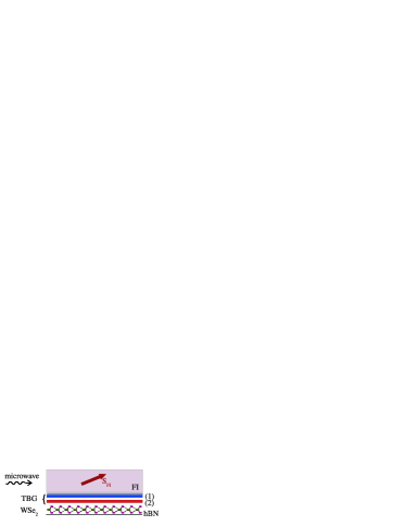
We theoretically study a planar junction of a FI and a TBG adjacent to (TBG/) as depicted in Fig. 1.
We consider the case where a microwave of a frequency is applied to this junction, and focus on the twist angle dependence of the FMR linewidth temp .
Figure 1: Schematic representation of the junction between a ferromagnetic insulator (FI) and a heterostructure of TBG adjacent to a monolayer of . The labels (1) and (2) denote the graphene layers of TBG represented by the red and the blue lines. The red arrow indicates the spin orientation of the FI characterized by an average spin , written in the coordinate frame of the FI magnetization. The gray lines represent the boron-nitride (hBN) layers encapsulating the TBG/ heterostructure.
Continuum model. – In TBG with a twist angle , the Hamiltonian of a graphene layer (), rotated at an angle , is
,
where and is the unrotated monolayer Hamiltonian. In the continuum limit, reduces to , where is the Fermi velocity, , and () are the sublattice-Pauli matrices and is the valley index. We assume that the SOC is only induced in the graphene layer adjacent to the TMD layer, since the SOC arises from overlaps between atomic orbitals Zaletel . This assumption is consistent with recent studies on bilayer graphene and TBG aligned on TMD layers Alex ; Gmitra-BL ; Zaletel ; Alex2 .
Layer (2), in contact with the monolayer, is then descried by the Hamiltonian
Alex , where is given by
(1)
() are the spin-Pauli matrices, , and correspond, respectively, to the Ising, Rashba and Kane-Mele SOC parameters Alex . The variation ranges of these parameters are , , while is expected to be small SOC1 ; SOC2 ; Makk ; Zaletel ; Wang ; Morpu16 ; SOC7 . The last term in is due to the inversion symmetry breaking induced by the TMD layer. Hereafter, we neglect this term regarding the small value of compared to the SOC parameters Alex .
As in the case of TBG Mc11 , the low-energy Hamiltonian of TBG/ reduces, at the valley , to
(2)
is written in the basis
constructed on the four-component spin-sublattice spinor and , () corresponding, respectively, to layer and layer (see Secs. I and II of the Supplemental Material supp and Refs. Mc11 ; Koshino18 ; Bernevig ; Falko19 ; Bi ; Alex ; Marwa ). The momentum is measured relatively to the Dirac point of layer (1). In Eq. (2), are the spin-independent interlayer coupling matrices, , () where are the vectors connecting to its three neighboring Dirac points of layer (2) in the moiré Brillouin zone (mBZ) Mc11 , and are given by
,
, ,
where is the mBZ basis (see Sec. I of the Supplemental Material supp ).
In the unrelaxed TBG, and choosing sublattice A as the origin of the unit cell in each layer, the matrices take the form Bernevig
,
and supp , where w is the interlayer tunneling amplitude and is the identity matrix acting on the sublattice indices.
Using the perturbative approach of Ref. Mc11 , we derive, from Eq. (2), the effective low-energy Hamiltonian of TBG/ (see Sec. II of the Supplemental Material supp ). To the leading order in , reads as supp
(3)
(4)
(5)
where , , , is the graphene lattice constant and
, () act now on the band indices of the eigenenergies of , denoted , and given to the leading orders in and by
(6)
Equation 5 shows that the SOC parameters and are renormalized by the moiré structure of TBG to
(7)
which increase by decreasing the twist angle.
The expression of [Eq. (3)] can be taken as a starting point to unveil the role of SOC in the emergence of the stable superconducting phase observed, at , in TBG adjacent to Alex .
To probe the validity of the effective Hamiltonian [Eq. (3)], we compared the corresponding eigenenergies with the numerical band structure obtained within the continuum model and taking into account 148 bands per valley and spin projection (see Sec. II of the Supplemental Material supp ). The results show that describes correctly the band structure of TBG/ down to a twist angle . At smaller angles, the effective Fermi velocities of are overestimated. Such a discrepancy is expected since the lattice relaxation effect is important at small angles Alex . It is worth noting that, for the sake of simplicity, we did not consider a relaxed TBG, since we are interested in the SP around the MA.
Gilbert damping. – In the absence of a junction, the magnon Green function of the FI is defined as Ohnuma ; Matsuo18 ; Kato19 ; Kato20 ; Matsuo-JP ; Matsuo20 ; Yama
, where are the Matsubara frequencies for bosons, is the amplitude of the average spin per site, and is the GD strength. The term describes the spin relaxation within the FI.
In FMR experiments, the microwave excitation induces a uniform spin precession, which limits the magnon self-energy to the processes with Funato .
In the presence of the interfacial coupling, a correction, , to the GD term is induced by the adjacent heterostructure TBG/. can be expressed in terms of the the self-energy , resulting from the interfacial exchange interactions, as Funato
(8)
For simplicity, we neglect the real part of which simply shifts the FMR line and did not affect the linewidth, in which we are interested.
The self-energy, in Eq. (8), includes the contributions of all the interfacial spin transfer processes and can be written as . Each process, described by the self-energy , is characterized by a momentum transfer and a matrix element .
In the second order perturbation, with respect to the interfacial exchange interaction , the self-energy , is written as Yama
(9)
are the electronic spin ladder operators written in the coordinate system of the FI magnetization characterized by an average spin .
is the electronic Matsubara Green function given by ,
where are the fermionic Matsubara frequencies. In the basis of the spin-band four-component spinor Alex , reads as
,
where are the spin-Pauli matrices; , , and () are expressed, to the leading order in the SOC, as a function of the band-Pauli matrices (see Sec. III of the Supplemental Material supp ).
Since the ferromagnetic peak, given by , is sharp enough, namely , one can replace the resonance frequency by the FMR frequency . The GD correction can then be expressed as Yama ; supp
(10)
In general, the interfacial spin transfer includes clean and dirty processes. The former (latter) take place with conserved (non-conserved) electron momentum, which turns out to take () in Eq. (9Funato ).
We first consider a clean interface, for which an analytical expression of the GD correction [Eq. 10] can be derived (see Sec. IV of the Supplemental Material supp and reference Funato ; Yama ). The case of a dirty junction is discussed in the next section.
Carrying out the summation over in Eq. (9), we obtain the analytical expression of the interfacial self-energy (see Sec. IV of the Supplemental Material supp ). The sum over the electronic states runs over the states included within a cutoff, , on the momentum amplitude , where the low-energy Hamiltonian [Eq. (3)] is expected to hold (see Sec. IV of the Supplemental Material supp ).
In the following, we discuss the behavior of the normalized GD coefficient
(11)
where is a dimensionless function depending on the twist angle , temperature , the chemical potential and the orientation of the FI magnetization, and is the average SOC (for details, see Sec. IV of the Supplemental Material supp and reference Guinea22 ).
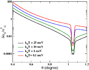
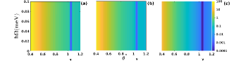
Discussion. – In Fig. 2, we plot [Eq. (11)], as a function of the twist angle , for the undoped TBG, at different temperatures and for a fixed FMR energy which corresponds to the yttrium iron garnet. The SOC parameters are and as in Ref. [Alex, ].
Figure 2: Normalized GD, [Eq. (11)], as a function of the twist angle at different temperature ranges. Calculations are done for , , , and for a FMR energy .
Figure 2 shows that regardless of the temperature range, increases by decreasing but drops sharply at the MA, where it exhibits a relatively small peak which is smeared out at low temperature.
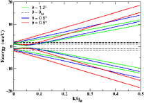
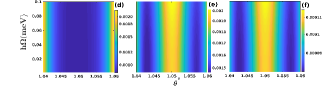
Putting aside its drop at the MA, the enhancement of , by decreasing , can be, in a first step, ascribed to the dependence of the self-energy [Eq. (9)] on the effective SOC, given by Eq. (7), which increase by decreasing . However, to understand the behavior of at the MA one needs to go back to the band structure, [Eq. (6)], of the continuum Hamiltonian of TBG/, which is depicted in Fig. 3 at different twist angles. The arrows indicate the out-of-plane electronic spin projection which we have numerically calculated for different twist angles in Sec. II of the Supplemental Material supp .
Away from the MA, the band dispersion gets larger as decreases and, in particular, the separation between bands with opposite , involved in the SP process, increases. This behavior is due to the angle dependence of the effective Fermi velocity of TBG/, which reduces, in the first order in the SOC, to that of TBG, namely (see Secs. I and II of the supplemental Material supp )
(12)
The expression of the GD [Eq. (11)] includes transitions between bands with opposite (see Sec. IV of the Supplemental Material supp ). These transitions depend on the statistical weight where is the Fermi-Dirac function and is the energy band with a spin orientation .
Figure 3: Band structure of TBG/ in the continuum limit [Eq. (6)] at (a), (b), (c) and (d). The dashed lines represent the bands at the MA (). The red (blue) arrows correspond to the out-of-plane electronic spin projection () Alex . Calculations are done for and .
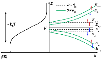
In Fig. 4, we plot a pictorial representation of the band structure of the continuum model [Eq. (6)] and the Fermi-Dirac distribution at a given temperature .
The band dispersion gets larger as moves away from the MA (Fig. 3) and
the separation between the bands with opposite increases.
As a consequence, the corresponding statistical weight is enhanced compared to the case around the MA.
This behavior explains the drop of the GD at the MA.
Around the MA ( and ), the statistical weight is reduced compared to that at the MA since the bands and get closer (Fig. 3).
This behavior gives rise to the small peak at the MA (Fig. 2), which disappears at low temperature () where bands around the MA have the same statistical weight (see Sec. IV of the Supplemental Material supp ). In this case, the GD is basically dependent on the effective Fermi velocity [Eq. (12)] which vanishes at exactly the MA. Such dependence is responsible for the cancellation of several terms contributing to the self-energy [Eq. (9)], as they are proportional to [Eq. (12)] (see Sec. IV of the Supplemental Material supp ).
Figure 4: Schematic representation of the band structure (Eq. 6) and the Fermi-Dirac distribution . The bands in dashed and green lines correspond, respectively, to the MA and to a twist angle far from the MA. The red (blue) arrows represent the projection of the out-of-plane spin projection ().
Around the MA, the bands are almost flat and the statistical weights , corresponding to the transitions between
and , are small compared to the case of a twist angle away from the MA, where the band dispersion is larger.
Let us now turn to the case of a dirty interface where the spin transfer should now also include the non-conserved momentum processes. The corresponding self-energy [Eq. (9)] can also be expressed in terms of the thermal weight governing the interband transitions (see Sec. IV of the Supplemental Material supp ).
Regarding the flatness of the bands, the dirty processes at the MA acquire, as in the clean limit, small thermal weights compared to the twist angles away from the MA, where the band are dispersive.
In the dirty limit, the Gilbert damping correction is, then, expected to drop at the MA as found in the case of a clean interface.
It comes out that the twist angle dependence of is a direct probe of the emergence of the flat bands in TBG. On the other hand, the temperature dependence of the fine structure around the MA provides an accurate measurement of the MA, with a precision below (see Fig. \colorredS.4 of the Supplemental Material supp ). It also gives an estimation of the SOC induced in TBG adjacent to a monolayer of TMD.
It is worth stressing that in our model we did not take into account the electron-electron interactions which significantly distort the electronic band structure of TBG Guinea18 ; Guinea20 ; Guinea21 ; Guinea22 . Near the MA, the dominant electron-electron interaction is found to be the Coulomb interaction with an amplitude estimated to be 10-15 meV Guinea20 , which is larger than the width of the flat bands meV and the SOC considered in the present work. How are the results of Fig.2 modified in the presence of Coulomb interaction?
Treating this interaction within the Hartree-Fock approximation revealed that the Hartree term considerably widens the bands while the exchange term leads, basically, to broken-symmetry phases. At the charge neutrality, the Hartree term vanishes and the exchange potential, which concerns bands with identical spins, opens a gap of 4 meV Guinea20 ; Guinea21 ; Guinea22 , which is of the order of the SOC amplitudes. As a consequence, the statistical weight of the bands with opposite is expected to increase, but keeping larger values at small angles compared to the MA. Moreover, the bandwidth, around the MA, is found to relatively increase under the exchange term Guinea20 ; Guinea21 ; Guinea22 , but remains smaller than 3 meV, which preserve the flatness of the bands. It comes out, that our results hold in undoped TBG under Coulomb interaction, and can be used to extract the value of the MA at which the Gilbert damping correction drops.
Away from the neutrality, the bands are substantially distorted by the Coulomb interaction Guinea20 ; Guinea21 ; Guinea22 and our results should be taken with a grain of salt since they account for filling factors away from , where the bandwidth, at the MA, is less than 4 meV.
Besides interactions, strain is found to be a key parameter in the emergence of flat bands in TBG Bi ; Marwa . The effect of strain can be included in our model by deriving the strain induced correction to the Hamiltonian given by Eq. (3), taking into account the strain dependence of the vectors connecting the Dirac points Marwa . The twist angle, at which drops, can then provide a way to measure the strain in TBG.
Experimental realization. –
Our proposed setup consists of an interface between a FI and a fully hBN encapsulated TBG/ heterostructure (Fig. 1).
The hBN layer acts as a tunnel barrier which prevents the diffusion of the FI atoms into the graphene layer SP-Gr .
On the other hand, the encapsulation provides a clean interface and prevents the graphene degradation SP-Gr which is a challenging issue in the STM and ARPES experiments Utama ; Efetov21 ; Sato , carried out on non-encapsulated TBG samples.
It should be stressed that the hBN encapsulated TBG/ heterostructure has been already realized in Refs. [Lin, ; Alex, ].
Furthermore, the spin transport through a clean interface between a FI and 2D material has been experimentally achieved SP-Gr ; SP-TMD . The 2D materials were fully encapsulated by hBN SP-Gr or covered by a thin layer of an oxide insulator (as MgO) SP-TMD to avoid the interdiffusion with the FI.
Our proposed technique to measure the MA can, then, be implemented experimentally with a clean interface and at room temperature.
Moreover, an insitu manipulation of the twist angle can be realized as in Refs. [Rebeca, ; Hu, ; Geim, ; Inbar, ].
Conclusion. – To conclude, we have proposed an experiment to probe the flat bands of TBG and to measure its MA accurately. The experiment is based on a spin pumping measurement through a junction separating a FI and a TBG adjacent to a monolayer of .
We first derived the continuum model of TBG with SOC, which constitutes a first step to develop an analytical understanding of the emergence of a stable superconducting state at small twist angles observed in TBG in proximity to Alex .
We then determined analytically the Gilbert damping correction induced by the presence of the TBG/ heterostructure.
Our results show that the twist angle dependence of exhibits a drop at the MA with a temperature-dependent fine structure. This feature provides an accurate determination of the MA and an estimation of the SOC induced in TBG by its proximity to the TMD layer. Our proposed set-up can be readily implemented regarding the state-of-the art of the experimental realizations of SP in 2D materials and TBG-based heterostructure.
Our work opens the gate to a twist tunable spintronics in twisted layered heterostructures.
Acknowledgments. –
We thank Mamoru Matsuo and Shu Zhang for stimulating discussions. We are indebted to Jean-Noël Fuchs and Daniel Varjas for a critical reading of the manuscript.
S. H. acknowledges the kind hospitality of the Institute for Solid State Physics (ISSP) where this work was carried out. S. H. also thanks the hospitality of the Max Planck Institute for the Physics of Complex Systems (MPI-PKS). S. H. acknowledges financial support from the ISSP International visiting professors program and the MPI-PKS visitors program.
References
(1) Y. Cao, V. Fatemi, S. Fang, K. Watanabe, T. Taniguchi, E. Kaxiras, and P. Jarillo-Herrero, Unconventional superconductivity in magic-angle graphene superlattices, Nature, 556, 43 (2018).
(2) Y. Cao, V. Fatemi, A. Demir, S. Fang, S. L. Tomarken, J. Y. Luo, J. D. Sanchez-Yamagishi, K. Watanabe, T. Taniguchi, E. Kaxiras, R. C. Ashoori, and P. Jarillo-Herrero, Correlated insulator behaviour at half-filling in magic-angle graphene superlattices, Nature, 556, 80 (2018).
(3) M. Yankowitz, S. Chen, H. Polshyn, Y. Zhang, K. Watanabe, T. Taniguchi, D. Graf, A. F. Young, C. R. Dean, Tuning superconductivity in twisted
bilayer graphene, Science 363, 1059 (2019).
(4) N. B. Kopnin, T. T. Heikkila, and G. E. Volovik, High-temperature surface superconductivity in topological flat-band systems, Phys. Rev. B 83, 220503(R) (2011).
(5) H. C. Po, L. Zou, A. Vishwanath, and T. Senthil, Origin of Mott Insulating Behavior and Superconductivity in Twisted Bilayer Graphene, Phys. Rev. X 8, 031089 (2018).
(6) F. Wu, A. H. MacDonald, and I. Martin, Theory of Phonon-Mediated Superconductivity in Twisted Bilayer Graphene, Phys. Rev. Lett. 121, 257001 (2018).
(7) B. Roy and V. Juricic, Unconventional superconductivity in nearly flat bands in twisted bilayer graphene, Phys. Rev. B 99, 121407(R) (2019).
(8) B. Lian, Z. Wang, and B. A. Bernevig, Twisted Bilayer Graphene: A Phonon-Driven Superconductor, Phys. Rev. Lett. 122, 257002 (2019).
(9) P. Stepanov, I. Das, X. Lu, A. Fahimniya, K. Watanabe, T. Taniguchi, F. H. L. Koppens, J. Lischner, L. Levitov and D. K. Efetov, Untying the insulating and superconducting orders in magic-angle graphene, Nature 583, 375 (2020).
(10) Y. Saito, J. Ge, K. Watanabe, T. Taniguchi, A. F. Young, Independent superconductors and correlated insulators in twisted bilayer graphene, Nature Physics 16, 926 (2020).
(11) Y. Cao, D. Rodan-Legrain, J. M. Park, F. N. Yuan, K. Watanabe, T. Taniguchi, R. M. Fernandes, L. Fu, P. Jarillo-Herrero, Nematicity and competing orders in superconducting magic-angle graphene, Science, 372, 264 (2021).
(12) X. Lu, P. Stepanov, W. Yang, M. Xie, M. A. Aamir, I. Das, C. Urgell, K. Watanabe, T. Taniguchi, G. Zhang, A.
Bachtold, A. H. MacDonald, and D. K. Efetov, Superconductors, orbital magnets and correlated states in magic-angle bilayer graphene, Nature
574, 653 (2019).
(13) H. Polshyn, M. Yankowitz, S. Chen, Y. Zhang, K.
Watanabe, T. Taniguchi, C. R. Dean, and A. F. Young, Large linear-in-temperature resistivity in twisted bilayer graphene,
Nat. Phys. 15, 1011 (2019).
(14) Y. Cao, D. Chowdhury, D. Rodan-Legrain, O.
Rubies-Bigorda, K. Watanabe, T. Taniguchi, T. Senthil,
and P. Jarillo-Herrero, Strange Metal in Magic-Angle Graphene with near Planckian Dissipation, Phys. Rev. Lett. 124, 076801
(2020).
(15) S. L. Tomarken, Y. Cao, A. Demir, K. Watanabe, T. Taniguchi, P. Jarillo-Herrero, and R. C. Ashoori, Electronic Compressibility of Magic-Angle Graphene Superlattices,
Phys. Rev. Lett. 123, 046601 (2019).
(16) G. Li, A. Luican, J. M. B. Lopes dos Santos, A. H. Castro Neto, A. Reina, J. Kong and E. Y. Andrei, Observation of Van Hove singularities in twisted graphene layers, Nature Physics, 6, 109 (2010).
(17) A. Kerelsky, L. J. McGilly, D. M. Kennes, L. Xian, M. Yankowitz, S. Chen, K. Watanabe, T. Taniguchi, J. Hone, C. Dean, A. Rubio and A. N. Pasupathy, Maximized electron interactions at the magic angle in twisted bilayer graphene, Nature, 572, 95 (2019).
(18) Y. Xie, B. Lian, B. Jäck, X. Liu, C.-L. Chiu, K. Watanabe, T. Taniguchi, B. A. Bernevig, and A. Yazdani, Spectroscopic signatures of many-body correlations in magic-angle twisted bilayer graphene, Nature
572, 101 (2019).
(19) Y. Choi, J. Kemmer, Y. Peng, A. Thomson, H. Arora, R. Polski, Y. Zhang, H. Ren, J. Alicea, G. Refael, F. von
Oppen, K. Watanabe, T. Taniguchi, and S. Nadj-Perge, Electronic correlations in twisted bilayer graphene near the magic angle,
Nat. Phys. 15, 1174 (2019).
(20) D. Wong, K. P. Nuckolls, M. Oh, B. Lian, Y. Xie, S. Jeon, K. Watanabe, T. Taniguchi, B. A. Bernevig, and A.
Yazdani, Cascade of electronic transitions in magic-angle twisted bilayer graphene, Nature 582, 198 (2020).
(21)Y. Choi, H. Kim, Y. Peng, A. Thomson, C. Lewandowski, R. Polski, Y. Zhang, H. S. Arora, K. Watanabe, T.
Taniguchi, J. Alicea, and S. Nadj-Perge, Correlation-driven topological phases in magic-angle twisted bilayer graphene, Nature
589, 536 (2021).
(22) N. Tilak, X. Lai, S. Wu, Z. Zhang, M. Xu, R. de Almeida Ribeiro, P. C. Canfield and E. Y. Andrei, Flat band carrier confinement in magic-angle twisted bilayer graphene, Nat Commun. 12, 4180 (2021).
(23) D. Călugăru, N. Regnault, M. Oh, K. P. Nuckolls, D. Wong, R. L. Lee, A. Yazdani, O. Vafek, and B. A. Bernevig, Spectroscopy of Twisted Bilayer Graphene Correlated Insulators, Phys. Rev. Lett. 129, 117602 (2022).
(24) M. I. B. Utama, R. J. Koch, K. Lee, N. Leconte, H. Li, S. Zhao, L. Jiang, J. Zhu, K. Watanabe, T. Taniguchi et al., Visualization of the flat electronic band in twisted bilayer graphene near the magic angle twist, Nat. Phys. 17, 184 (2021).
(25) S. Lisi, X. Lu, T. Benschop, T. A. de Jong, P. Stepanov, J. R. Duran, F. Margot, I. Cucchi, E. Cappelli, A. Hunter, et al., Observation of flat bands in twisted bilayer graphene, Nat. Phys. 17, 189 (2021).
(26) K. Sato, N. Hayashi, T. Ito, N. Masago, M. Takamura, M. Morimoto, T. Maekawa, D. Lee, K. Qiao, J. Kim, et al., Observation of a flat band and bandgap in millimeter-scale twisted bilayer graphene, Commun Mater 2, 117 (2021).
(27) Y. Tserkovnyak, A. Brataas, and G. E. W. Bauer, Enhanced Gilbert Damping in Thin Ferromagnetic Films, Phys. Rev. Lett. 88, 117601 (2002).
(28) Y. Tserkovnyak, A. Brataas, G. E. W. Bauer, and B. I. Halperin, Nonlocal magnetization dynamics in ferromagnetic heterostructures, Rev. Mod. Phys. 77, 1375 (2005).
(29) Maekawa, Sadamichi and others (eds), Spin Current, 1st edn, Series on Semiconductor Science and Technology (Oxford, 2012; online edn, Oxford Academic, 17 Dec. 2013), https://doi.org/10.1093/acprof:oso/9780199600380.001.0001.
(30) F. Hellman, A. Hoffmann, Y. Tserkovnyak, G. S. D. Beach, E. E. Fullerton, C. Leighton, A. H. MacDonald, D. C. Ralph, D. A. Arena, H. A. Dürr el al., Interface-induced phenomena in magnetism, Rev. Mod. Phys. 89, 025006 (2017).
(31) Z. Qiu, J. Li, D. Hou, E. Arenholz, A. T. N’Diaye, A. Tan, K.-i. Uchida, K. Sato, S. Okamoto, Y. Tserkovnyak, Z. Q. Qiu, and E. Saitoh, Spin-current probe for phase transition in an insulator, Nat. Commun. 7, 12670 (2016).
(32) F. Yang and P. C. Hammel, FMR-driven spin pumping in Y3
Fe5O12-based structures, J. Phys. D Appl. Phys. 51, 253001 (2018).
(33) W. Han, S. Maekawa, and X. Xie, Spin current as a probe of quantum materials, Nat. Mater. 19, 139 (2020).
(34) S. Hait, S. Husain, H. Bangar, L. Pandey, V. Barwal, N. Kumar, N. K. Gupta, V. Mishra, N. Sharma, P. Gupta, et al., Spin Pumping through Different Spin-Orbit Coupling Interfaces in -W/Interlayer/Co2FeAl Heterostructures, ACS Appl. Mater. Interfaces 14, 37182 (2022).
(35) A. Avsar, J. Y. Tan, T. Taychatanapat, J. Balakrishnan, G. K. W.
Koon, Y. Yeo, J. Lahiri, A. Carvalho, A. S. Rodin, E. C. T.
O’Farrell, G. Eda, A. H. Castro Neto, and B. Özyilmaz, Spin-orbit proximity effect in graphene, Nat.
Commun. 5, 4875 (2014).
(36) Z. Wang, D.-K. Ki, H. Chen, H. Berger, A. H. MacDonald, and A. F. Morpurgo, Strong interface-induced spin-orbit interaction in graphene on WS2, Nat. Commun. 6, 8339 (2015).
(37) Z. Wang, D.-K. Ki, J. Y. Khoo, D. Mauro, H. Berger, L. S. Levitov, and A. F. Morpurgo, Origin and Magnitude of ‘Designer’ Spin-Orbit Interaction in Graphene on Semiconducting Transition Metal Dichalcogenides, Phys. Rev. X 6, 041020 (2016).
(38) B. Yang, M.-F. Tu, J. Kim, Y. Wu, H. Wang, J. Alicea, R. Wu, M. Bockrath, and J. Shi, Tunable spin-orbit coupling and symmetry-protected edge states in graphene/WS2, 2D Mater. 3, 031012 (2016).
(39) W. Yan, O. Txoperena, R. Llopis, H. Dery, L. E. Hueso, and F. Casanova, A two-dimensional spin field-effect switch, Nat. Commun. 7, 13372 (2016).
(40) B. Yang, M. Lohmann, D. Barroso, I. Liao, Z. Lin, Y. Liu, L. Bartels, K. Watanabe, T. Taniguchi, and J. Shi, Strong electron-hole symmetric Rashba spin-orbit coupling in graphene/monolayer transition metal dichalcogenide heterostructures, Phys. Rev. B 96, 041409(R) (2017).
(41) T. S. Ghiasi, J. Ingla-Aynés, A. A. Kaverzin, and B. J. van Wees, Large Proximity-Induced Spin Lifetime Anisotropy in Transition-Metal Dichalcogenide/Graphene Heterostructures, Nano Lett. 17, 7528 (2017).
(42) A. Dankert and S. P. Dash, Electrical gate control of spin current in van der Waals heterostructures at room temperature, Nat. Commun. 8, 16093 (2017).
(43) T. Völkl, T. Rockinger, M. Drienovsky, K. Watanabe, T. Taniguchi, D. Weiss, and J. Eroms, Magnetotransport in heterostructures of transition metal dichalcogenides and graphene, Phys. Rev. B 96, 125405 (2017).
(44) S. Zihlmann, A. W. Cummings, J. H. Garcia, M. Kedves, K. Watanabe, T. Taniguchi, C. Schönenberger, and P. Makk, Large spin relaxation anisotropy and valley-Zeeman spin-orbit coupling in
WSe2/graphene/-BN heterostructures, Phys. Rev. B 97, 075434 (2018).
(45) T. Wakamura, F. Reale, P. Palczynski, S. Guéron, C. Mattevi, and H. Bouchiat, Strong Anisotropic Spin-Orbit Interaction Induced in Graphene by Monolayer WS2, Phys. Rev. Lett. 120, 106802 (2018).
(46) J. C. Leutenantsmeyer, J. Ingla-Aynés, J. Fabian, and B. J. van Wees, Observation of Spin-Valley-Coupling-Induced Large Spin-Lifetime Anisotropy in Bilayer Graphene, Phys. Rev. Lett. 121, 127702 (2018).
(47) S. Omar and B. J. van Wees, Spin transport in high-mobility graphene on WS2 substrate with electric-field tunable proximity spin-orbit interaction, Phys. Rev. B 97, 045414 (2018).
(48) L. A. Benítez, J. F. Sierra, W. S. Torres, A. Arrighi, F. Bonell, M. V. Costache, and S. O. Valenzuela, Strongly anisotropic spin relaxation in graphene–transition metal dichalcogenide heterostructures at room temperature, Nat. Phys. 14, 303 (2018).
(49) C. K. Safeer, J. Ingla-Aynés, F. Herling, J. H. Garcia, M. Vila, N. Ontoso, M. R. Calvo, S. Roche, L. E. Hueso, and F. Casanova, Room-Temperature Spin Hall Effect in Graphene/MoS2 van der Waals Heterostructures, Nano Lett. 19, 1074 (2019).
(50) J. O. Island, X. Cui, C. Lewandowski, J. Y. Khoo, E. M. Spanton, H. Zhou, D. Rhodes, J. C. Hone, T. Taniguchi, K. Watanabe, L. S. Levitov, M. P. Zaletel and A. F. Young, Spin-orbit-driven band inversion in bilayer graphene by the van der Waals proximity effect, Nature 571, 85 (2019).
(51) D. Wang, S. Che, G. Cao, R. Lyu, K. Watanabe, T. Taniguchi, C. Ning Lau, and M. Bockrath, Quantum Hall Effect Measurement of Spin–Orbit Coupling Strengths in Ultraclean Bilayer Graphene/WSe2 Heterostructures, Nano Lett. 19, 7028 (2019).
(52) T. Wakamura, F. Reale, P. Palczynski, M. Q. Zhao, A. T. C. Johnson, S. Guéron, C. Mattevi, A. Ouerghi, and H. Bouchiat, Spin-orbit interaction induced in graphene by transition metal dichalcogenides, Phys. Rev. B 99, 245402 (2019).
(53) A. David, P. Rakyta, A. Kormányos, and G. Burkard, Induced spin-orbit coupling in twisted graphene–transition metal dichalcogenide heterobilayers: Twistronics meets spintronics,
Phys. Rev. B 100, 085412(2019).
(54) T. Wang, N. Bultinck, and M. P. Zaletel, Flat-band topology of magic angle graphene on a transition metal dichalcogenide,
Phys. Rev. B 102, 235146 (2020).
(55) For a review see, T. Wakamura, S. Guéron and H. Bouchiat, Novel transport phenomena in graphene induced by strong spin-orbit interaction, Comptes Rendus. Physique, 22, 145 (2021).
(56) H. S. Arora, R. Polski, Y. Zhang, A. Thomson,
Y. Choi, H. Kim, Z. Lin, I. Z. Wilson, X. Xu,
J. -H. Chu, K. Watanabe, T. Taniguchi, J. Alicea and S. Nadj-Perge, Superconductivity in metallic twisted bilayer graphene stabilized by WSe2, Nature 583 379 (2020).
(57) J.-X. Lin, Y.-H. Zhang, E. Morissette, Z. Wang, S. Liu, D. Rhodes, K. Watanabe, T. Taniguchi, J. Hone, J. I. A. Li, Spin-orbit–driven ferromagnetism at half moiré filling in magic-angle twisted bilayer graphene, Science 375, 437 (2022).
(58) S. Bhowmik, B. Ghawri, Y. Park, D. Lee, S. Datta, R. Soni, K. Watanabe, T. Taniguchi, A. Ghosh, J. Jung, and U. Chandni, Spin-orbit coupling-enhanced valley ordering of malleable bands in twisted bilayer graphene on WSe2, Nature Communications 14, 4055 (2023).
(59) We consider the relatively high temperature regime compared to the critical temperatures at which emerge the strongly correlated insulating states of TBG () Herrero1 , or the ferromagnetic phase observed, at , in TBG aligned to Lin .
(60) Y. Zhang, R. Polski, A. Thomson, E. Lantagne-Hurtubise, C. Lewandowski, H. Zhou, K. Watanabe, T. Taniguchi, J. Alicea and S. Nadj-Perge, Enhanced superconductivity in spin-orbit proximitized bilayer graphene, Nature 613, 268 (2023).
(61) M. Gmitra, and J. Fabian, Proximity Effects in Bilayer Graphene on Monolayer WSe2: Field-Effect Spin Valley Locking, Spin-Orbit Valve, and Spin Transistor, Phys. Rev. Lett. 119, 146401 (2017).
(62) M. Gmitra, and J. Fabian, Graphene on transition-metal dichalcogenides: A platform for proximity spin-orbit physics and optospintronics, Phys. Rev. B 92, 155403 (2015).
(63) M. Gmitra, D. Kochan, P. Hogl, and J. Fabian, Trivial and inverted Dirac bands and the emergence of quantum spin Hall states in graphene on transition-metal dichalcogenides, Phys. Rev. B 93, 155104 (2016).
(64) A. W. Cummings, J. H. Garcia, J. Fabian, J. and S. Roche, Giant Spin Lifetime Anisotropy in Graphene Induced by Proximity Effects, Phys. Rev. Lett. 119, 206601 (2017).
(65) R. Bistritzer and A. H. MacDonald, Moiré bands in twisted double-layer graphene, Proc. Natl. Acad. Sci.U.S.A., 108, 12233 (2011).
(66) For details, see the Supplemental Material including detailed derivations of the continuum model of TBG/WSe2 [Eq. (3)] and the correction to the Gilbert damping coefficient [Eq. (11)], numerical calculations of the band structure of TBG/WSe2 and the behavior of the Gilbert damping coefficient as a function of different model parameters.
(67) D. A. Ruiz-Tijerina and V. I. Fal’ko, Interlayer hybridization and moiré superlattice minibands for electrons and excitons in heterobilayers of transition-metal dichalcogenides, Phys. Rev. B 99, 125424 (2019).
(68) Z. Bi, N. F. Q. Yuan, and L. Fu, Designing flat bands by strain, Phys. Rev. B 100, 035448 (2019).
(69) M. Koshino, N. F. Q. Yuan, T. Koretsune, M. Ochi, K. Kuroki, and L. Fu, Maximally Localized Wannier Orbitals and the Extended Hubbard Model for Twisted Bilayer Graphene, Phys. Rev. X 8, 031087 (2018).
(70) M. Mannaï and S. Haddad, Twistronics versus straintronics in twisted bilayers of graphene and transition metal dichalcogenides, Phys. Rev. B 103, L201112 (2021) and references therein.
(71) G. Cantele, D.Alfè, F. Conte, V. Cataudella, D. Ninno, and P. Lucignano, Structural relaxation and low-energy properties of twisted bilayer graphene, Phys. Rev. Research 2, 043127 (2020).
(72) Y. Ohnuma, H. Adachi, E. Saitoh, and S. Maekawa, Enhanced dc spin pumping into a fluctuating ferromagnet near
, Phys. Rev. B 89, 174417 (2014).
(73) M. Matsuo, Y. Ohnuma, T. Kato, and S. Maekawa, Spin Current Noise of the Spin Seebeck Effect and Spin Pumping, Phys. Rev. Lett. 120, 037201 (2018).
(74) T. Kato, Y. Ohnuma, M. Matsuo, J. Rech, T. Jonckheere, and T. Martin, Microscopic theory of spin transport at the interface between a superconductor and a ferromagnetic insulator, Phys. Rev. B 99, 144411 (2019).
(75) T. Kato, Y. Ohnuma, and M. Matsuo, Microscopic theory of spin Hall magnetoresistance, Phys. Rev. B 102, 094437 (2020).
(76) Y. Ominato and M. Matsuo, Quantum Oscillations of Gilbert Damping in Ferromagnetic/Graphene Bilayer Systems, J. Phys. Soc. Jpn. 89, 053704 (2020).
(77) Y. Ominato, J. Fujimoto, and M. Matsuo, Valley-Dependent Spin Transport in Monolayer Transition-Metal Dichalcogenides, Phys. Rev. Lett. 124, 166803 (2020).
(78) M. Yama, M. Tatsuno, T. Kato, and M. Matsuo, Spin pumping of two-dimensional electron gas with Rashba and Dresselhaus spin-orbit interactions,
Phys. Rev. B 104, 054410 (2021).
(79)T. Funato, T. Kato, and M. Matsuo, Spin pumping into anisotropic Dirac electrons, Phys. Rev. B 106, 144418 (2022).
(80) T. Cea, P. A. Pantaleón, N. R. Walet and F. Guinea, Electrostatic interactions in twisted bilayer graphene, Nano Materials Science 4, 27 (2022) and references therein.
(81) F. Guinea and N. R. Walet, Electrostatic effects, band distortions, and superconductivity in twisted graphene bilayers, PNAS 115, 13174 (2018).
(82) T. Cea and F. Guinea, Band structure and insulating states driven by Coulomb interaction in twisted bilayer graphene, Phys. Rev. B 102, 045107 (2020).
(83) T. Cea and F. Guinea, Coulomb interaction, phonons, and superconductivity in twisted bilayer graphene, PNAS 118, e2107874118 (2021).
(84) M. Gurram, S. Omar, S. Zihlmann, P. Makk, C. Schönenberger, and B. J. van Wees, Spin transport in fully hexagonal boron nitride encapsulated graphene, Phys. Rev. B 93, 115441 (2016).
(85) Z. Zhou, P. Marcon, X. Devaux, P. Pigeat, A. Bouché, S. Migot, A. Jaafar, R. Arras, M. Vergnat, L. Ren, Large Perpendicular Magnetic Anisotropy in Ta/CoFeB/MgO on Full-Coverage Monolayer MoS2 and First-Principles Study of Its Electronic Structure, ACS Appl. Mater. Interfaces, 13, 32579 (2021).
(86) R. Ribeiro-Palau, C. Zhang, K. Watanabe, T. Taniguchi, J. Hone, C. R. Dean, Twistable electronics with dynamically rotatable heterostructures, Science 361, 690 (2018).
(87) C. Hu, T. Wu, X. Huang, Y. Dong, J. Chen, Z. Zhang, B. Lyu, S. Ma, K. Watanabe, T. Taniguchi, et al., In-situ twistable bilayer graphene, Scientific Reports 12, 204 (2022).
(88) Y. Yang, J. Li, J. Yin, S. Xu, C. Mullan, T. Taniguchi, K. Watanabe, A. K. Geim, K. S. Novoselov, A. Mishchenko, In situ manipulation of van der Waals heterostructures for twistronics, Sci. Adv. 6, eabd3655 (2020).
(89) A. Inbar, J. Birkbeck, J. Xiao, T. Taniguchi, K. Watanabe, B. Yan, Y. Oreg, A. Stern, E. Berg and S. Ilani, The quantum twisting microscope, Nature 614, 682 (2023).
SUPPLEMENTAL MATERIAL
Twisted bilayer graphene reveals its flat bands under spin pumping
Sonia Haddad1,2,3, Takeo Kato2, Jihang Zhu3, and Lassaad Mandhour1
1Laboratoire de Physique de la Matière Condensée, Faculté des Sciences de Tunis, Université Tunis El Manar, Campus Universitaire 1060 Tunis, Tunisia
2 Institute for Solid State Physics, University of Tokyo, Kashiwa, Chiba 277-8581, Japan
3 Max Planck Institute for the Physics of Complex Systems, Nöthnitzer Strasse 38, Dresden 01187, Germany
S.1 I. Derivation of the low-energy Hamiltonian of TBG without SOC
We start by a brief overview of the perturbative approach proposed by Bistritzer and MacDonald Mc11 to derive the continuum model of TBG. We consider a TBG where the two layers are rotated oppositely . The Hamiltonian of a graphene layer rotated at an angle is
(S.1)
where is the Hamiltonian of the unrotated layer given, in the continuum limit, by
(S.2)
where the momentum is written relatively to the Dirac point ,
is the Fermi velocity, is the valley index, and () are the sublattice-Pauli matrices.
The leading contributions of the interlayer tunneling can be limited to three nearest hopping processes in the momentum space connecting states , around the Dirac point of layer , to the states around , the Dirac point of layer . The vectors are given by Mc11
(S.3)
where and , being the graphene lattice parameter. The is the moiré BZ basis given by , are the lattice basis vectors of the monolayer reciprocal lattice and .
is the rotation tensor written, in the sublattice basis, at a small twist angle as
(S.4)
In the basis , the Hamiltonian, at the valley , reads as Mc11
(S.5)
For the relaxed TBG the matrices are given by Koshino18
(S.6)
Here is given by Eq. S.1 and , where the momentum is written relatively to .
and is the shortest inplane shifts between carbon atoms of the two layers Bernevig ; Falko19 .
Hereafter, we neglect the relative sliding between the layers which is not relevant in the physics of TBG Mc11 ; Bernevig .
Choosing the A sublattice in both layers () as the origin of the unit cell, turns out to take in Eq. S.6Bernevig .
The parameters , and are the tunneling amplitudes which take the same value in the rigid TBG Bi .
In the relaxed lattice, these amplitudes are no more equal meV and meV Koshino18 .
In the present work, we do not consider the lattice relaxation effect, since the SOC parameters are small compared to the difference between the interlayer amplitudes .
In the unrelaxed lattice, the matrices can be written as
(S.7)
Here, is the identity matrix acting on the sublattice indices.
Considering, in Eq. S.5, the dependent term as a perturbation, the effective Hamiltonian can be written, to the leading order in , as
(S.8)
where is the zero energy eigenstate of . is constructed on the two-component sublattice spinor () of layer (layer ) taken at the momentum () around the Dirac point () at the valley . is the zero energy eigenstate of .
The components satisfy
(S.9)
where . Then
(S.10)
To the leading order in , , takes the following form
(S.11)
(S.12)
Eq. S.12 is obtained by neglecting in , which turns out to take in Mc11 .
is the effective velocity of the energy band of TBG around the zero energy which vanishes at the MA , and is given by Mc11
(S.13)
where , .
In our numerical calculations (Fig. \colorred3 of the main text), we take and which corresponds to for the first MA Mc11 .
S.2 II. Derivation of the low-energy Hamiltonian of TBG with SOC
We now consider the heterostructure consisting of TBG adjacent to a monolayer of as shown in Fig.1 of the main text, where we denote the graphene layer in contact with the TMD by layer (2). This layer is subject to a SOC induced by proximity effect by the TMD, and the corresponding Hamiltonian can be written as Alex
(S.14)
where is given by Eq. \colorred1 of the main text.
To derive the continuum model of TBG/, we follow the perturbative approach of Ref. Mc11 presented in the previous section. Now, the basis is constructed on the four-component spin-sublattice spinor and , () corresponding, respectively, to layer and layer .
is written as
. In this basis, the Hamiltonian of TBG/ takes the form
(S.15)
The momentum is measured relatively to the Dirac point of layer (1), , () and includes now the SOC terms (Eq. S.14).
We take the sublattice A as the origin of the unit cell in each layer. The matrices are written as the tensor product of those given by Eq. S.7, with the identity spin-matrix .
Regarding the small values of the SOC, we assume that has a zero eigenenergy and the corresponding eigenstate satisfies the condition given by Eq. S.10.
Following the same procedure as in the previous section, we derive from Eq. S.11 the effective low energy Hamiltonian of TBG/ by substituting by the Hamiltonian of layer (2), rotated at and including SOC as
(S.16)
Hereafter, we neglect the Kane and Mele term whose contribution, to the leading order in , is found to vanish. We also disregard the last term in Eq. S.16, which results into a higher order correction in .
To the first order in the SOC coupling, we obtain the continuum model of TBG/ described by the Hamiltonian given by Eq. \colorred3 in the main text.
This Hamiltonian contain a SOC term () with renormalized Ising and Rashba interactions
(S.17)
and are enhanced by decreasing the twist angle from the MA.
Figure S.1: Energy bands of TBG/ around zero energy as function of the dimensionless momentum amplitude at different twist angles. The bands are represented up to the cutoff . Calculations are done for and Alex . The MA is .
To the leading order in , the four eigenergies of the Hamiltonian (Eq. \colorred3 of the main text), denoted , are given by
(S.18)
(S.19)
where is the band index. are depicted in Fig. S.1 at different twist angles.
At the Dirac point, the eigenergies reduce to
(S.20)
It is worth to note that in TBG, the flatness of the bands around the charge neutrality point strongly depends on the heterostrain which may emerge in the graphene layers during the fabrication procedure Marwa . The interplay between strain and SOC in TBG/ goes beyond the scope of the present work.
In figures S.2 and S.3, we plot the electronic band structure of TBG/ at different twist angles. The solid lines correspond to the numerical results obtained within the continuum model taking into account 148 bands for each spin and valley. The calculations are done for the relaxed TBG with interlayer momentum hopping amplitudes and (Eq. S.6). We considered these values to reproduce the numerical band structure obtained in Ref.[ Alex, ] using the continuum model. We have taken into account the lattice relaxation, as in Ref. Alex, , since it is expected to be important at small angles.
The numerical results are compared to the eigenergies of the effective Hamiltonian , given by Eq. \colorred3 of the main text (dashed line), and to the approximated expressions (Eq. S.18) represented by dotted gray lines. It should be stressed that is derived for a rigid TBG, for which we have taken an interlayer hopping amplitude , which gives rise to a MA as in Ref [Alex, ].
For the sake of simplicity, we did not consider the relaxation effect, which is not significant around the MA Alex , where we consider the spin pumping effect. The derivation of the effective Hamiltonian of the relaxed TBG adjacent to is left to a future work.
Figure S.2: Electronic band structure of TBG/ calculated, at a twist angle (a) , (b) , and (c) . Calculations are based on the continuum model and including 148 bands for each moiré valley and spin. The line color denotes the value of the out-of-plane spin projection .
The dashed black lines represent the eigenergies of the four-band effective Hamiltonian given by Eq. \colorred3 of the main text, and the gray dotted lines denote the approximated eigenergies given by Eq. S.18. Calculations are done for and . The band structure is represented in the moiré Brillouin zone where and correspond respectively to the Dirac point of layer (1) and layer (2) at the valley . The bottom panel is a zoomed-in representation around the high symmetry point .Figure S.3: Electronic band structure of TBG/ calculated around the MA at (a) , (b) , (c) . The bottom panel is a zoomed-in representation around the high symmetry point .
The data are the same as in Fig. S.2.
As shown by Fig. S.2 and S.3, the effective Hamiltonian (Eq. \colorred3 of the main text) provides a good description of the band structure of TBG/. It can be taken as a framework to unveil the origin of the observed stable superconducting state in this heterostructure Alex .
However, at relatively small angles (), the Fermi velocities of are overestimated (Fig. S.2). This discrepancy is due to the assumption of a rigid TBG lattice which is not justified at small angles Alex .
S.3 III. Electronic Green function
The Matsubara Green function associated to the effective Hamiltonian (Eq. \colorred5) is
(S.21)
where and are the spin and band identity matrices, respectively.
can be expressed as
(S.22)
are spin-Pauli matrices, and the components () of are written as
(S.23)
The and operators are written in terms of the band-Pauli matrices and the corresponding identity matrix
(S.24)
here and .
In the limit of small SOC couplings , A, B, C, and D become
S.4.1 Interfacial exchange coupling between a ferro-
magnetic insulator (FI) and a TBG
We consider the Hamiltonian of the ferromagnetic insulator (FI) in the independent magnon approximation as
(S.41)
where is a dispersion of magnons, is a spin stiffness, is the gyromagnetic ratio, is a static magnetic field.
In the spin pumping setup, only the static part associated to is relevant.
Considering only the uniform spin precession, the Hamiltonian of the FI can be simply written as
(S.42)
where is the Fourier transformation of the site representation defined as
(S.43)
(S.44)
where is the number of unit cells in the FI.
We consider the (retarded) magnon Green function as
(S.45)
(S.46)
In the absence of the junction, the magnon Green function is
(S.47)
We introduce spin relaxation of the bulk FI phenomenologically as
(S.48)
where is a dimensionless strength of the Gilbert damping, which is of order of –.
We note that a line shape of the ferromagnetic resonance is proportional to Funato .
In the presence of the interfacial coupling and for a uniform spin precession, the magnon Green function is given by the Dyson equation as
(S.49)
where is the self-energy.
Although the real part of is related to the shift of the ferromagnetic resonance, we neglect it for simplicity.
Then, the magnon Green function is rewritten as
(S.50)
(S.51)
We note that depends on in general.
However, since the ferromagnetic resonance peak is sharp enough (), we can replace with (the peak position of the ferromagnetic resonance):
(S.52)
The Hamiltonian of the interfacial coupling is given as
(S.53)
Here, is a spin ladder operator of the FI and is described by magnon annihilation/creation operators ( and ) as
(S.54)
where is an amplitude of the localized spin in the FI.
is a spin ladder operator of electrons in two-dimensional electron systems (twisted bilayer graphene) and is described by the electron annihilation/creation operators ( and ) as
(S.55)
We define the Fourier transformation as
(S.56)
(S.57)
where is the number of unit cells and is the position of the site in TBG.
Then, we obtain
(S.58)
(S.59)
We define the Fourier transformation of as
(S.60)
(S.61)
From , we obtain the relation .
The inverse Fourier transformation is given as
For a clean interface, we can set .
Then, using Eqs. (S.43) and (S.44), the Hamiltonian of the interface is written as
(S.67)
where is defined as
.
By the second-order perturbation, the self-energy of the magnon at is calculated as
(S.68)
(S.69)
The self-energy can be related to a retarded component of the dynamic spin susceptibility per unit cell as
(S.70)
(S.71)
(S.72)
is calculated for one-band of TBG without spin-orbit interaction as
(S.73)
where , is a dispersion of electrons, is a chemical potential.
This is just a Lindhard function.
We note that is independent of the system size (area).
For systems with spin-orbit interaction, we have to extend the Lindhard function into the spin-dependent one.
Then, the enhancement of the Gilbert damping is written as
(S.74)
We note that the number of the unit cell of twisted bilayer graphene is written as where is a area of the junction and is an area of a unit cell of twisted bilayer graphene.
We also note that the number of the unit cell of the FI is written as where is a thickness of the FI, is a lattice constant of the FI.
Using these parameters, we obtain
(S.75)
We note that is proportional to in consistent with experimental results.
If YIG (Yttrium Iron Garnet) is chosen as the ferromagnet insulator, the parameter is given in the Table.
Table 1: Experimental parameters.
Microwave frequency
Amplitude of spins of FI
10
Lattice constant of FI
Å
Thickness of FI
Interfacial exchange coupling
(not known)
S.4.2 Electronic spins in the FI magnetization frame
Regarding the dependence on of the electronic Hamiltonian (Eq. \colorred3 of the main text), one should consider a FI magnetization as in Ref. Funato . The average spin vector is along the orthoradial spherical vector . The radial vector forms an angle with the axis perpendicular to the interface. The third axis is in the plane and its unit vector is the orthoradial inplane vector as shown in Fig.S.4.
Figure S.4: Magnetization-fixed coordinate frame with respect to the Laboratory frame .
In the FI spin frame (), the components of the electronic spin operators are given by:
We define the ladder electronic spin operators as
(S.77)
where .
S.4.3 Magnon self-energy
In the second order perturbation with respect to the interfacial exchange interaction , the interfacial self-energy is given by Yama
(S.78)
where is the electronic Green function given by Eq. S.22.
The trace term is of the form:
(S.79)
where the vector is written in the laboratory frame .
We set and .
Taking into account the operator character of one could use the identity
(S.80)
Given the expressions of and in Eq. S.23, the trace term (Eq. S.79) reduces to:
(S.81)
where
(S.82)
The terms with a prime are expressed in terms of .
Regarding the dependence of the and operators (Eqs. S.3- S.40), only , the last term in and the three first terms in give non-vanishing contributions after summing over in Eq. \colorred12.
On the other hand, the terms between parentheses in the first and second line in expression give the same contribution.
As a result, the GD is found to be independent of the azimuthal angle , which expresses isotropy of the electronic band structure (Eq. S.18). However, the GD depends on the out-of-plane orientation of the FI magnetization via the angle .
According to Eq. S.78, the terms to calculate are of the form
Taking the analytic continuation , Eq. S.83 becomes
(S.86)
being the Lorentzian function. The sum over in Eq. S.86 reduces to , where is the moiré superlattice area, is a cutoff on the momentum amplitude , below which the continuum model for the monolayer is justified. We take , where is the separation between the Dirac points and of, respectively, layer (1) and layer (2) at a given monolayer valley .
S.4.4 Gilbert damping correction
For a uniform spin precession, the Gilbert damping correction , at the FMR frequency , can be expressed as Yama
(S.87)
The imaginary part of the self-energy is of the form , where is a dimensionless integral.
Introducing the average SOC , can be written as
(S.88)
where .
In Fig. S.5, we plot the normalized Gilbert damping correction as a function of the twist angle and the FMR energy at different temperatures. The bottom panels are a zoomed representation around the MA.
Fig. S.5 shows that, the GD increases by decreasing the twist angle and sharply drops at the MA, regardless of the temperature range and the FMR frequency .
At high temperature (), the GD exhibits, around the MA, a fine structure characterized by a peak which disappears at low temperature.
The origin of this peak is, as discussed in the main text, due to the dispersion of the energy bands of TBG/ and their corresponding thermal weights (Eq. S.86).
Figure S.5: Color plot of the normalized Gilbert damping correction as a function of the twist angle and the FMR energy at ((a) and (d)), ((b) and (e)) and ((c) and (f)). The bottom panels show the behavior of the GD around the MA.
Calculations are done for , and .
In Fig. S.6 we plot corresponding to the transitions between and in the case of the undoped system.
Figures S.6 (a) and (b) show that, at high temperature (), increases as the band dispersion gets larger and reaches its minimal value at the MA. This behavior explains the drop of the GD at the MA and its enhancement at small twist angles.
In figure S.6 (c), we plot around the MA, at relatively high thermal energy compared to the SOC, where the GD exhibits a peak at the MA (Fig. \colorred2 of the main text).
In this case, is maximal at the MA and decreases at the angles and close to the MA.
This feature results from the decrease of the energy separation between and at and , compared to that at (Fig. \colorred3 of the main text). At low temperature, and around the MA, one gets for the transitions and . As a consequence, the GD behavior is now only dependent on the effective Fermi velocity which vanishes at the MA. As a consequence, the small peak of the GD, emerging at the MA at relatively high temperature, disappears.
Figure S.6: Statistical weight corresponding to the transitions between (a) and ((b) and (c)) at different temperatures.
The dots represent the energy (a) and ((b) and (c)) at the MA and the arrows mark the limit of the band (a) and ((b) and (c)) at the indicated twist angle. In (c), is shown around the MA for the transition between . Calculations are done for the SOC , Alex and in the undoped TBG ().
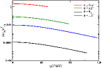
Figure S.7 shows the behavior of the normalized GD correction as function of the chemical potential at and for the FMR energy . The decrease of is a consequence of the thermal weight.
The results shown in Fig. S.7 are expected to hold in the presence of Coulomb interaction if the width of the bands at the MA remains less than 4 meV, which is the case of the filling factor satisfying Guinea22 .
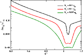
Figure S.7: Normalized GD correction as function of the chemical potential at and for different twist angles. The upper limit of is corresponding to the momentum cutoff . Calculations are done for the SOC , Alex , and for the FMR energy .Figure S.8: Normalized GD correction as function of the SOC and at a twist angle (a), (b) and at the MA (c). Calculations are done for , and for the FMR energy .
In Fig. S.8, we plot the normalized GD correction as function of the SOC parameters, and , for different twist angles, at , and in the case of the undoped system. The drop of at the MA is a robust feature regardless of the amplitude of the SOC. However, there is a relative increase of , at the MA, if the bands and (or and ) are in resonance with the FMR energy, as shown in Fig. S.8(c). This resonance can be only reached for relatively small values of .
As shown in Fig. S.2, the energy spectrum of the effective model (dashed lines) are slightly more dispersive, at small twist angles (), than those obtained by including higher bands (solid lines). This discrepancy should be taken into account when fixing the value of the cutoff up to which the sum in Eq. S.86 is evaluated. To determine the role of the cutoff on the SP effect, we plot, in Fig. S.9, the GD correction as a function of the twist angle at different cutoffs , where is the momentum separation between the Dirac points and of respectively layer (1) and layer (2) at a given valley .
Fig. S.9 shows that the GD correction drops at the MA regardless of the cutoff values. The larger the cutoff, the sharper the drop.
Figure S.9: Normalized GD correction as function of the twist angle for different values of the cutoff parameter . Calculations are done for , , , , and for the FMR energy .