Artificial Intelligence and Dual Contract

Abstract

With the dramatic progress of artificial intelligence algorithms in recent times, it is hoped that algorithms will soon supplant human decision-makers in various fields, such as contract design. We analyze the possible consequences by experimentally studying the behavior of algorithms powered by Artificial Intelligence (Multi-agent Q-learning) in a workhorse dual contract model for dual-principal-agent problems. We find that the AI algorithms autonomously learn to design incentive-compatible contracts without external guidance or communication among themselves. We emphasize that the principal, powered by distinct AI algorithms, can play mixed-sum behavior such as collusion and competition. We find that the more intelligent principals tend to become cooperative, and the less intelligent principals are endogenizing myopia and tend to become competitive. Under the optimal contract, the lower contract incentive to the agent is sustained by collusive strategies between the principals. This finding is robust to principal heterogeneity, changes in the number of players involved in the contract, and various forms of uncertainty.

JEL classification: D21, D43, D83, L12, L13

Keywords: Artificial intelligence, dual contract, principal-agent problem, AI alignment.

1 Introduction

Platforms are increasingly adopting Artificial Intelligence (henceforth, AI) algorithms (for example, the ChatGPT (Ouyang et al. (2022)) and Eloundou et al. (2023)) to intelligentize services and price their products, and this tendency is likely to be extended to other business areas, particularly contract design. In this paper, we ask whether contracting algorithms may ”autonomously” learn to be incentive compatible, especially for the contracting problem with multiple sides, which we also refer to as the multi-sided contracting problem. We emphasize that AI algorithms can be used to automatically optimize the terms of a contract by taking into account the preferences of both sides and the legal and economic environment in which the agreement must be implemented. Note that this contract negotiation process is automatic, requiring very little external guidance.

In light of these developments, concerns have been voiced by scholars and organizations alike, that AI algorithms may create an AI alignment problem due to differences between the specified reward function and what relevant humans (the designer, the user, others affected by the agent’s behavior) actually value (see Hadfield-Menell and Hadfield (2019) and Gabriel (2020)). We highlight that this AI alignment problem has a clear analogy to the principal-agent problem (see Hadfield-Menell and Hadfield (2019)), and the analysis of incentive compatibility for the incomplete contracting via AI algorithms can provide an insightful framework for understanding the alignment among algorithms.

But how real is the risk of misalignment among AI algorithms? That is a difficult question to answer, both empirically and theoretically. On the empirical side, alignment is notoriously hard to detect from market outcomes, and firms typically do not disclose details of the financial or employment contracts they have. On the theoretical side, the interaction among reinforcement-learning algorithms in dynamic agency problems generates dynamic stochastic multi-agent systems so complex that analytical results seem currently out of reach.

To make some progress, this paper takes an experimental approach. The possibility arises from the recent evolution of AI algorithms from rule-based to multi-agent reinforcement learning (hereafter referred to as MARL) programs, which are able to learn from data and adapt to changing environments. We construct AI-based principals and agents, thereby allowing them to interact repeatedly in computer-simulated marketplaces. The challenge of this approach is to choose reasonable economic environments and algorithms that are representative of those used in realistic contract design scenarios. Specifically, we start from a conventional principal-agent problem as a reference and thereafter consider a three-sided contracting problem, where the parties have different preferences for the contract terms, also referred to as the dual-contract problem. To this end, the MARL algorithms tackle the ”Dual-Contract” problem and analyze its performance regarding its ability to learn incentive-compatible contract; our findings do suggest that algorithmic incentive compatibility is more than a remote theoretical possibility.

To clarify the basic contribution of this paper, we start by comparing the following concepts

• Classical Principal-Agent Problem is a well-studied issue in economics and contract theory. It arises when one side (the principal) delegates decision-making authority to another side (the agent). The principal provides the resources and capital for the project, while the agent is responsible for completing it. Incentives must be set by the principal to ensure that the project is completed efficiently and effectively. This two-sided problem has been studied extensively in the literature and applied to various areas.

• Dual-Contracting Problem is a three-sided version of the classical principal-agent problem. In this case, there are two principals: both project owners provide resources and capital for the project. The two principals can have the same or different objectives and interests, which need to be colluded or competed with in order to ensure that the project is completed efficiently and effectively. This problem has rarely been studied in the literature, particularly in dynamic scenarios, as solving the three (or more)-agent Markov games remain a challenge for conventional methods. To our knowledge, this paper can also be recognized as the first investigation of the well-defined dual-contracting problem via novel methods. such as AI algorithms.

• AI for Mechanism Design have been proposed to detect the mechanism design problem via AI algorithms (e.g., Calvano et al. (2020)). These algorithms are typically multi-agent reinforcement learning (MARL) programs, which are able to learn from data and adapt to multi-agent interactions. These algorithms can be used to optimize the terms of a mechanism design problem and detect the AI’s behavior, in order to maximize the expected utility of both sides.

Along with investigating the AI alignment problem, we are interested in studying how to design contracts by AI algorithms for three alternative reasons. Firstly, it might be applicable to online contracting scenarios, especially for decentralized multi-sided platforms.

Second, when online contracting occurs in decentralized platforms, it is common for agents to rely on incentive optimization tools provided by the decentralized systems (blockchain or smart contract). As Web 3.0 applications become more popular, it is a natural question to ask how to compete in such contracts that would evolve when multiple agents use similar algorithmic tools, each optimizing on behalf of its owner.

Third, understanding how AI algorithms interact with contract design can help us to design contracts more effectively for AI-driven applications. By understanding how AI algorithms interact with contract design, we can create contracts that incentivize the desired behavior of the AI algorithm. Additionally, understanding how AI algorithms interact with contract design can help us better identify and mitigate potential risks associated with related AI-driven applications.

The dual-contracting problem is a challenging one due to the complexity of the task and the need for both principals to coordinate their efforts. To tackle this problem, AI algorithms have been proposed to learn from data and adapt to multi-agent interactions. Starting from a dynamic version of the static moral hazard model as a benchmark reference model, we find that the proposed relatively simple contracting algorithms dynamically learn to play incentive-compatible strategies and catch up with a rule-based reference analytical model solution in terms of the number of iterations needed to reach a Nash equilibrium. The baseline case indicates that, indeed, the initial conditions are no longer relevant to the equilibrium outcome given the same environment setup.

In this paper, the main difference between the classical principal-agent problem and the dual-contracting problem is that the former is a single-principal problem, which cannot account for the mixed-sum behavior (collusion or competition) between principals and their effect on contract design. To understand the economic forces behind the dual-contract problem, we can notice multiple differences between the standard principal-agent problem and dual-contract problem formats that can contribute to different outcomes. This is because the dual-contract problem can induce multi-sided information asymmetry. In particular, we point out that:

• Principals gain reduced benefits if their contract incentives are misaligned.

• The principal reacts to changes in the behavior of other participants, including agents and other principals.

• Advantageous principals get protection from competition and enjoy increased benefits.

The AI-based principles typically coordinate on contract incentive designs that are somewhat above the pure collusion equilibrium (single principal-agent equilibrium), but substantially above the pure competition equilibrium. The strategies that generate these outcomes involve an intelligent level of AI algorithms, which is reflected in their memory ability. These algorithms learn these strategies through trial and error, and those with higher memory capacity can guard against myopic preferences and make better choices in the long term. Remarkably, these AI-based principals are not designed or instructed to collude or compete; they do not communicate with one another, nor do they have prior knowledge of the environment in which they operate.

Our baseline model is a symmetric duopoly principal with an agent, and we conduct an extensive robustness analysis for the principal’s heterogeneity. The results indicates that, the principal has an advantage over another principal and can get protection from his competitor; this protection effect increases as the degree of competition rises. Specifically, this protection effect results in the tax rate $p$ (benefit rate to the principal) is much higher than zero in the pure competition region, increasing the profit for the principal with advantage without worry about the competition from another principal. Moreover, in the pure collusion region, the two principals divide the revenue from both contracts evenly; therefore, both principals would like the agent to put effort into the advantaged principal’s project.

We designed a series of experiments/simulations to tell these possible explanations apart. It turns out that the main reason for the difference is the fact that there are multiple principals, and there are different levels of how much the principals’ interests are aligned with each other. This force is fundamentally different between the standard contract and the dual-contract problems. It also helps us understand why the multi-sided information asymmetry seems to lead to reduced overall benefit for a party suffering from a conflict of interest among its members.

This work provides proof of concept that AI algorithms can be used to autonomously learn incentive compatibility in contract design. The proposed multi-agent reinforcement learning (MARL) algorithm is a promising approach to the problem of contract design and negotiation, as it can autonomously learn incentive compatibility and reach a Nash equilibrium in a reasonable number of iterations. This work could be extended to other multi-sided contracting problems, such as the three-sided problem, and other AI algorithms, such as deep reinforcement learning. Furthermore, the proposed MARL algorithm could be used to optimize the terms of a contract to maximize the expected utility for both sides.

Additionally, AI algorithms is hopefully to identify potential risks associated with a given contract and suggest mitigation changes. Alternatively, AI algorithms can help automate the contract negotiation process by offering terms most likely to be accepted by both sides, potentially leading to faster and more efficient contract negotiations and reducing the costs associated with the process. Ultimately, AI algorithms can help organizations make better decisions when designing and negotiating contracts, resulting in better outcomes for both sides.

1.1 Related Literature

Our paper contributes to the literature by proposing a MARL algorithm to solve the dual-contract problem and demonstrating its ability to learn incentive compatibility autonomously. The proposed algorithm is a promising tool for contract design, as it can help organizations make better decisions when online designing and negotiating contracts.

The literature on the use of AI algorithms to solve the mechanism design problem is still in its infancy. However, there have been some recent works that have explored this topic. For example, Banchio and Skrzypacz (2022) proposed an autonomous AI-based auction design using a reinforcement learning algorithm. Hansen et al. (2021) show how misspecified implementation results in collusion by simulating a different algorithm from the bandit literature. In contrast to those works, the present paper is the first to explore the use of AI algorithms to solve the dual-contracting problem with incentive compatibility. We propose a MARL algorithm to solve the dual-contracting problem and analyze its performance regarding its ability to learn incentive compatibility. Our results suggest that AI algorithms can be used to autonomously learn incentive compatibility in dual-contract design.

This paper contributes to an emerging literature that applies AI modeling in economics and finance. Recent literature in AI economics has been actively studying reinforcement learning that particularly utilizes the Q-learning method as the tool for experimental economics. These include Erev and Roth (1998), Kessler and Roth (2012), Calvano et al. (2020), Klein (2021), Kasy and Sautmann (2021), Asker et al. (2022), among many others. In contrast, our application of AI is motivated economically by the challenges observed in conventional dynamic contract theory and the pressing need for theoretically approximating humanity. We contribute conceptually by introducing a novel quantitative framework to solve the AI-based dual-contracting problem in a relatively transparent and interpretable modeling space.

This paper hopes to usefully complement the rich theoretical literature on optimal contracting and principal-agent problems, such as Innes (1990), Schmidt (1997), Levin (2003), DeMarzo and Sannikov (2006), DeMarzo and Fishman (2007), Biais et al. (2007), Sannikov (2008) He (2009), Biais et al. (2010), Garrett and Pavan (2012), DeMarzo et al. (2012), Edmans et al. (2012), Zhu (2013), Garrett and Pavan (2015), and Zhu (2018). The optimal contract in these papers is typically highly complex, and they must engage several bounded assumptions or conditions to ensure the model’s tractability. Note that most of these studies must suppose a specific scenario, such as one principal and one agent. In contrast, our paper considers a fairly general dual-contract setting with two principals and one agent, under a tractable AI setting, the model is to deliver quantitative analysis in a dynamic multi-period setting and calibrate the model parameters using real data.

Our paper is organized as follows. In Section Section 2, we provide a brief overview of Q-learning and multi-agent reinforcement learning. In Section 3, adopt a two-agent Q-learning algorithm to analyze the single-principal-agent problem. Section 4 describes our proposed multi-agent Q-learning algorithm for the dual-contracting problem. In Section 5, we present the results of the dual-contracting problem with heterogeneous principals. Section 6 concludes. The omitted algorithm details are presented in Appendix A.

2 Q-learning

We concentrate on Q-learning algorithms (see Watkins and Dayan (1992) and its application for economics Calvano et al. (2020)). Q-learning is a model-free reinforcement learning algorithm, which is also adopted for training artificial intelligence. It is an off-policy algorithm using a Q-value function to find the optimal action-selection policy. The Q-value function is a table that stores the expected utility of taking a given action in a given state. The algorithm updates the Q-value function based on the reward for taking action in a given state. The algorithm then uses the updated Q-value function to select the optimal action in the next state. The goal of the algorithm is to find the optimal policy that maximizes the expected reward.

This algorithm is based on reinforcement learning, a type of machine learning that focuses on taking suitable actions to maximize rewards. In this case, the rewards are associated with the choices made by the agent. The agent can then learn from its experiences and adjust its strategy accordingly. Q-learning assigns a value to each agent’s action and updates these values based on the rewards received. This allows the agent to learn from experiences and adjust its strategy accordingly. Using Q-learning, the agent can learn to make better decisions and maximize rewards. There are several reasons why we chose Q-learning: first, it is an algorithm commonly adopted in practice; second, it provides a logical simulation of decision making and learning processes; third, its parameters have clear economic interpretations which allow for comprehensive comparative statics analysis while minimizing modeling choices; fourth, it has similar structure to advanced programs that have recently achieved remarkable successes such as ChatGPT (Ouyang et al. (2022)). In this section we will briefly introduce Q-learning.

2.1 Single Agent Problems

Like all reinforcement-learning algorithms, Q-learning adjusts its behavior based on experience, taking actions that have been successful more often and those that have been unsuccessful less often. By using reinforcement learning, they can discover an optimal policy or policy close to optimal without prior knowledge of the specific problem.

Q-learning is a reinforcement learning algorithm initially used to solve Markov Decision Processes (MDPs) with finite states and actions. In this model, the agent interacts with the environment by acting in a given state and receiving a reward. The goal of Q-learning is to learn the optimal policy, which is the sequence of actions that maximizes the expected cumulative reward. Q-learning does not require state-dependent actions, meaning that the same action can be taken in different states. In a stationary Markov decision process, in each period $t=0,1,2,...$ an agent observes a state variable $s_{t}{\in}S$ and then chooses an action $a_{t}{\in}A(s_{t})$. For any $s_{t}$ and $a_{t}$, the agent obtains a reward $\pi_{t}$, and the system moves on to the next state $s_{t+1}$, according to a time-invariant (and possibly degenerate) probability distribution $F(\pi_{t},s_{t+1}|s_{t},a_{t})$. Q-learning deals with the version of this model where $S$ and $A$ are finite, and $A$ is not state-dependent.

The decision-maker’s problem is to maximize the expected present value of the reward stream:

$$E[\sum_{t=0}^{\infty}{\delta^{t}}\pi_{t}],$$ (2.1)

where $\delta\leq 1$ represents the discount factor. This dynamic programming problem is usually tackled using Bellman’s value function

$$V(s)=\max\{E[\pi|s,a]+{\delta}E[V(s^{\prime})|s,a]]\},$$ (2.2)

where s’ is a shorthand for $s_{t+1}$. Using Bellman’s value function, we can instead consider the Q-function, which represents the discounted payoff of taking action $a$ in state $s$, for our purposes. It is implicitly defined as

$$Q(s,a)=E(\pi|s,a)+{\delta}E[\max_{a^{\prime}{\in}A}Q(s^{\prime},a^{\prime})|s,a],$$ (2.3)

where the first term on the right-hand side is the period payoff, and the second term is the continuation value. The Q-function is related to the value function by the simple identity $V(s){\equiv}\max_{a{\in}A}Q(s,a)$. Since $S$ and $A$ are finite, the Q-function can be represented as an $|S|{\times}|A|$ matrix.

learning

Q-learning is used to determine the optimal action for a given state without knowing the underlying model. It does this by using trial and error to estimate the Q-matrix, which is a matrix that contains the expected rewards for each action taken in a given state. Once the Q-matrix is estimated, the agent can calculate the optimal action for any given state. Q-learning is essentially a method for estimating the Q-matrix without knowing the underlying model, i.e., the distribution function $F(\pi,s^{\prime}|s,a)$.

Q-learning algorithms use an iterative process to approximate the Q-matrix. The algorithm starts from an arbitrary initial matrix $Q_{0}$, after choosing action $a_{t}$ in state $s_{t}$, the algorithm observes $\pi_{t}$ and $s_{t+1}$ and updates the corresponding cell of the matrix $Q_{t}(s,a)$ for $s=s_{t},a=a_{t}$, according to the learning equation:

$$Q_{t+1}(s,a)=(1-\alpha)Q_{t}(s,a)+\alpha[\pi_{t}+{\delta}\max_{a{\in}A}Q_{t}(s^{\prime},a)],$$ (2.4)

according to equation (2.4), for the cell visited, the new value $Q_{t+1}(s,a)$ is a convex combination of the previous value and the current reward plus the discounted value of the state that is reached next. For all other cells $s{\neq}s_{t}$ and $a{\neq}a_{t}$, the Q-value does not change: $Q_{t+1}(s,a)=Q_{t}(s,a)$. The learning rate is the weight $\alpha\in[0,1]$. Its purpose is to regulate the learning process and determine how much experience is taken into account when estimating current action values. Watkins and Dayan (1992) demonstrated that Q-learning could converge to the optimal policy in a Markov Decision Problem (MDP) for a single agent. However, there is no assurance that this will work for generalized multi-agent Q-learning. Difficulties arise from the lack of stationarity: each agent is faced with an unpredictable, ever-evolving environment, and the reward distribution is dependent on the actions of their opponents. When the Markov property is not satisfied, various experiments in the literature have found that independent Q-learning can still be effective in such settings. In addition, opponent-aware algorithms necessitate more data about each opponent’s design and behavior, while the independent design approach maintains the reinforcement learning paradigm’s model-free simplicity.

Experimentation

All possible actions must be tested in all states to approximate the true matrix starting from an arbitrary $Q_{0}$. This requires exploring all possible combinations of states and actions to determine the best action for each state. The process of experimentation allows the algorithm to explore new possibilities and to learn from its mistakes, thus improving its performance over time. There is a cost associated with further exploration, necessitating a balance between utilizing the knowledge already gained and continuing to learn. Finding the optimal resolution to this trade-off can be difficult, but Q-learning algorithms do not attempt to optimize it. Instead, the mode and intensity of exploration are set externally. The $\epsilon$-greedy exploration policy is a simple approach for exploration in reinforcement learning. It involves selecting the optimal action with a fixed probability of $1-\epsilon$ and randomizing uniformly across all available actions with probability $\epsilon$. This approach allows for exploring different actions while exploiting the most rewarding activities. In this way, $1-\epsilon$ is the fraction of times the algorithm is in exploitation mode, while $\epsilon$ is the fraction of times it is in exploration mode. Even though more sophisticated exploration policies can be designed, our analysis will mainly focus on the $\epsilon$-greedy specification due to its simplicity.

3 Experiment Design

We begin with a heuristic naive case by constructing Q-learning algorithms and allowing them to interact in a dynamic contract setting, hoping that the naive case will illustrate that AI algorithms can learn incentive-compatible contracts automatically without any external guidance. To this end, we take Innes (1990) as the reference model for the naive case to examine the effectiveness and convergence of the AI outcomes. The selection of the reference model remains for the following important reasons:

• The model is tractable enough to obtain an analytical solution, providing a clear benchmark for evaluating the equilibrium outcomes of AI algorithms in the naive case.

• The setup of Innes (1990) is logically straight forward and easy to implement in the dynamic setting of the experiment environment for the AI algorithms.

• The Model is simple and can be fully characterized by just a few parameters, the economic interpretation of which is clear.

• The setup is suitable for progressing to the dynamic dual-contract scenario, making the dual-principal-agent problem remain well defined and interpretable yet difficult to be analyzed using conventional methods.

Note that learning a dynamic setting of such a static moral hazard model is not our goal in the current paper. The importance of selecting a parsimonious reference model is to prove the AI algorithms’ learnability of incentive-compatible contracts in a relatively tractable way, although we can choose more complicated models and build up more intricate experiment environments for the AI algorithm. Here, we describe the reference model and the economic environment in which the algorithms operate, the exploration strategy they follow, and other aspects of the numerical simulations.

3.1 Reference Model and Economic Environment

Specifically, a risk-neutral principal provides investment funds to a risk-neutral agent, who then makes an unobservable ex-ante effort choice. Its key idea is that legal liability limits bind the investment contract.

• Project requires initial investment $I$, which comes from principal.

• agent exerts unobservable effort $e$ at cost $\frac{1}{2}ce^{2}$

• With probability $e$, project generates payoff $X^{H}$.

• With probability $1-e$, generate payoff $X^{L}<X^{H}$.

• Contract pays principal $D^{L}$ if payoff is $X^{L}$ and $D^{H}$ if payoff is $X^{H}$.

• Agent retains the residual.

For a given contract $(D^{L},D^{H})$, the agent maximizes

$$e(X^{H}-D^{H})+(1-e)(X^{L}-D^{L})-\frac{1}{2}ce^{2},$$ (3.1)

The first-order condition for $e$ gives the incentive-compatible (IC) constraint:

$$(X^{H}-D^{H})+(X^{L}-D^{L})=ce,$$ (3.2)

The individual rationality (IR) constraint is that the principal must also break even, so we need

$$eD^{H}+(1-e)D^{L}=I,$$ (3.3)

Lagrangian for optimal contract

$$\mathcal{L} =e(X^{H}-D^{H})+(1-e)(X^{L}-D^{L})-\frac{1}{2}ce^{2}$$

$$+\lambda_{1}(e-\frac{(X^{H}-D^{H})-(X^{L}-D^{L})}{c}+\lambda_{2}(1-eD^{H}-(1-e)D^{L}),$$ (3.4)

Derivative wrt $D^{L}$

$$\frac{\mathrm{d}\mathcal{L}}{\mathrm{d}D^{L}}=-(1-e)-\frac{\lambda_{1}}{c}-\lambda_{2}(1-e),$$ (3.5)

Derivative wrt $D^{H}$

$$\frac{\mathrm{d}\mathcal{L}}{\mathrm{d}D^{H}}=-e+\frac{\lambda_{1}}{c}-e\lambda_{2}=-\frac{\mathrm{d}\mathcal{L}}{\mathrm{d}D^{L}}-(1+\lambda_{2}),$$ (3.6)

Claim

Optimal to set $D^{L}=X^{L}$.

Proof by contradiction

Suppose optimal $D^{L}<X^{L}$. Then it must be the case that $\frac{\mathrm{d}\mathcal{L}}{\mathrm{d}D^{L}}=0$.

• If it were not, we would increase $D^{L}$.

• But then we will have $\frac{\mathrm{d}\mathcal{L}}{\mathrm{d}D^{H}}<0$, so we will want to set $D^{H}=0$.

• But then we will induce negative effort.

• Instead, set $D^{L}=X^{L}$ and $X^{H}>D^{H}>I$.

3.2 Economic Environment

The reference model looks like a debt contract:

• At a low project payoff, the principal gets everything.

• At high project payoff, the agent gets residual.

• At high project payoff, the principal gets more than initially provided, which is similar to interest payment.

The key intuition is to reward the agent for a high project payoff that induces effort.

• Leave the agent with the max possible cash in that state.

• Compensate by giving the principal as much as possible in the low payoff state

We adopt the setup of the reference model to construct our economic environment. Here, we drop the IR constraint (Equation 3.3), as we would like to demonstrate that AI algorithms can autonomously learn to be rational individuals.

Setup

Single principal-agent contract Problem

• Project requires initial investment $I$, which comes from the principal.

• Principal chooses a “tax rate” $p{\in}[0,1]$.

• Agent observes principal’s “tax rate” then exerts effort $e{\in}[0,1]$ at cost $\frac{1}{2}ce^{2}$

• The project generates payoff $I+(T-I)e$, where $T$ is the highest possible payoff.

• Contract pays principal $I+(T-I)ep$.

• Agent retains the residual.

3.3 Parametrization and Initialization

Initially, we focus on a baseline economic environment that consists of a principal-agent problem with $T=2I$ and $c=2I$. For this specification, the profit $(T-I)e$ is equal to the agent’s cost $\frac{1}{2}ce^{2}$ when the agent’s effort is equal to $1$. This means that when the agent exerts effort $e=1$, the net profit will be equal to $0$.

As for the initial matrix $Q_{0}$, our baseline choice is to set the Q-values at $t=0$ to a random number between $0$ and $1$. The learning parameter $\alpha$ may be in the principal range from $0$ to $1$. It is well known, however, that high values of $\alpha$ may disrupt learning when experimentation is extensive as the algorithm would forget too rapidly what it has learned in the past. Learning must be persistent to be effective, requiring that $\alpha$ be relatively small. In machine learning literature, a value of $0.1$ is often used; accordingly, we choose $\alpha=0.1$ in our baseline model.

As for the experimentation parameter $\epsilon$, the trade-off is as follows. First, the algorithms need to explore extensively, as the only way to learn is through multiple visits to every state-action cell (of which there are $101$ in our baseline experiment with $|S|=1,|A|=101$, and much more in more complex environments). Additionally, exploration is costly. One can abstract from the short-run cost by considering long-run outcomes. But exploration also entails another cost if there is more than one algorithm learning, in that if one algorithm experiments more extensively, this creates noise in the environment, making it harder for the other to learn. This externality means that, in principle, experimentation may be excessive, even discounting the short-term cost.

Our baseline model adopts the $\epsilon$-greedy model with a time-invariant exploration rate. Although a more complex, time-declining exploration rate can be designed, a fixed exploration rate is enough for our purpose.

3.4 Results

In this part of the simulation, we simulate a Q-learning algorithm (the principal) contracting with the agent. The Q-learning algorithm needs to choose a “tax rate” $p$. The agent will observe this $p$ and act in their best interest. The grid of allowable choices of $p$ includes 101 $p$ levels from $0$ to $1$. The outcome of this experiment is reported in Figure 1. Expressly, we set $\epsilon=0.2$.

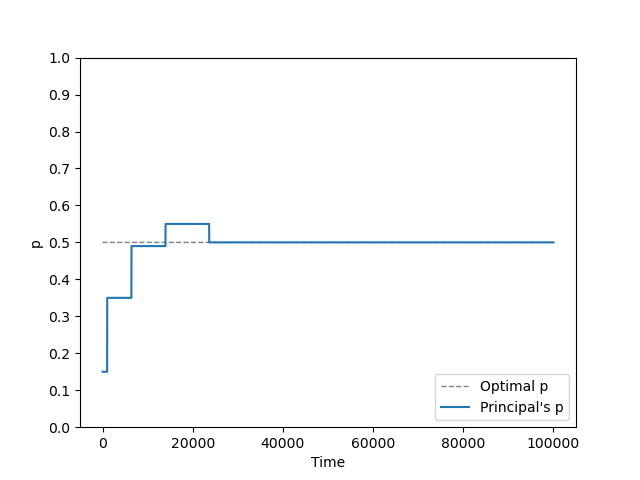
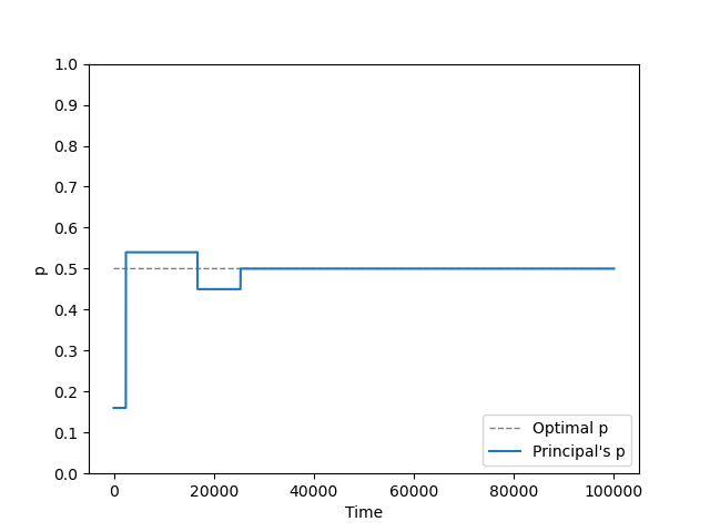
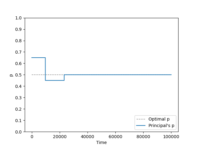
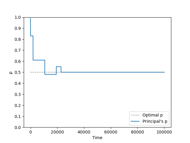
Figure 1: These pictures show the Q-learning algorithm gradually finding the optimal tax rate $p$.

Result

Our algorithm converges to the optimal choice of $p$. One thing to note in Figure 1 is that there exists a static optimal $p$. After finding this optimal $p$, there is no need for the algorithm to explore further. This is intuitive, as the agent always acts in their best interest and has a fixed strategy for every $p$ the principal chooses. However, this may not be true if there are more than one algorithm learning and they are playing against each other, as seen in the following dual contract problem.

4 Dual Contract Problem

A dual contract is an agreement between parties who have made two contracts for the same transaction. It can be an arrangement where an agent has two contracts with different principals. This is a situation in which an individual works for two employers simultaneously. This arrangement can be beneficial for both the agent and the principal, as it allows the agent to gain experience in different fields and the employers to benefit from the agent’s skills and knowledge. However, it is important to ensure that the two principals are aware of the arrangement and that the agent is not overworked or taken advantage of. The dual contract is used to ensure that both parties are legally bound to the same terms and conditions. It is also used to protect the interests of both parties in the event of a dispute.

In this section, we use Q-learning to solve dual contract problems based on the two-principal Innes Model. We first define the action space and reward function. The principal’s action space is defined as a discretized choice of “tax rate” $p$. The reward function is defined according to the rate of “identity of interests” $\beta$.

Next, we define the Q-learning algorithm. The algorithm starts by initializing the Q-table with random numbers. Then, for each state-action pair, the algorithm updates the Q-value using the Bellman equation. The algorithm then selects the action with the highest Q-value and performs the action. After performing the action, the algorithm updates the Q-table with the new reward. The algorithm then repeats the process until the goal is reached.

Finally, we test the Q-learning algorithm on the dual contract problem. We set the initial investment $I$ to $1$ and the initial highest possible payoff $T$ to $2$. We then run the Q-learning algorithm for $10000000$ iterations. The results show that the Q-learning algorithm is able to successfully solve the dual contract problem and reach the optimal solution.

4.1 Multi-agent Q-learning

Multi-agent reinforcement learning (MARL) is a sub-field of reinforcement learning. It is a type of reinforcement learning that involves multiple agents interacting with each other in an environment. The agents learn from each other and the environment to maximize their reward. This type of learning can be used to solve complex problems that require cooperation between multiple agents. It focuses on studying the behavior of multiple learning agents that coexist in a shared environment. Each agent is driven by its incentives, taking actions that benefit itself; in certain situations, these incentives may conflict with the interests of other agents, leading to intricate group behavior. MARL algorithms can be used to learn how to coordinate multiple agents to achieve a common goal, such as playing a game or navigating a complex environment.

In the dual contract problem, Multi-agent reinforcement learning is used to solve the problem. In this approach, each principal is a Q-learning algorithm trained to maximize its reward while considering the other principal’s behavior. When multiple agents act in a shared environment, their interests might be aligned or misaligned. MARL is a powerful tool for studying how different alignments of interests between multiple agents in a shared environment can affect their behavior. MARL allows us to explore the various alignments of interests between agents, such as cooperative, competitive, or mixed, and how these alignments can influence the agents’ behavior. By studying the effects of different alignments of interests, MARL can help us better understand how agents interact with each other in a shared environment. Specifically, we explore three settings:

• Pure competition region ($\beta=0)$: The principals’ rewards are opposite to each other, and therefore they are playing against each other.

• Pure collusion region ($\beta=0.5)$: The principals get the same rewards and therefore play with each other.

• Mixed-sum region ($0<\beta<0.5)$: It covers all the games that combine elements of both collusion and competition.

4.2 Setup

Dual contract Problem

• Project $1$ requires initial investment $I_{1}$, which comes from the principal $1$.

• Project $2$ requires initial investment $I_{2}$, which comes from the principal $2$.

• Principal $1$ chooses a “tax rate” $p_{1}{\in}[0,1]$.

• Principal $2$ chooses a “tax rate” $p_{2}{\in}[0,1]$ without observing $p_{1}$.

• Agent observes $p_{1}$ and $p_{2}$ then exerts effort $e_{1}{\in}[0,1]$ in project $1$ and effort $e_{2}{\in}[0,1]$ in project $2$ at cost $\frac{1}{2}c(e_{1}+e_{2})^{2}$, where ($e_{1}+e_{2}\leq 1$).

• Project $1$ generates payoff $I_{1}+(T_{1}-I_{1})e_{1}$, where $T_{1}$ is the highest possible payoff.

• Contract pays principal $1$: $I_{1}+(T_{1}-I_{1})e_{1}p_{1}$.

• Project $2$ generates payoff $I_{2}+(T_{2}-I_{2})e_{2}$, where $T_{2}$ is the highest possible payoff.

• Contract pays principal $2$: $I_{2}+(T_{2}-I_{2})e_{2}p_{2}$.

• Agent retains the residual.

4.3 Agent’s strategy

The agent observes the “tax rate” $p_{1}$ and $p_{2}$ two principals give and chooses the optimal effort in each project. Because the agent can select his action after observing $p_{1}$ and $p_{2}$, his strategy is unaffected by the learning process of the two principals. The agent’s strategy is determined by the preferences of the two principals, and the agent’s goal is to maximize his utility. Therefore, the agent’s strategy will be based on the preferences of the two principals, and the agent will choose the action that will maximize his utility. The agent’s strategy is not affected by the learning process of the two principals, as the agent’s strategy is determined by the preferences of the two principals, not by the learning process.

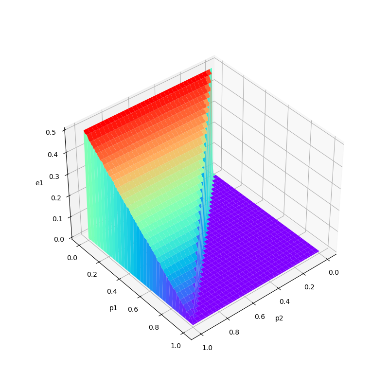
(a) Agent’s effort in project $1$

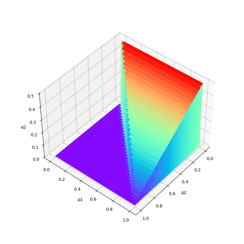
(b) Agent’s effort in project $2$

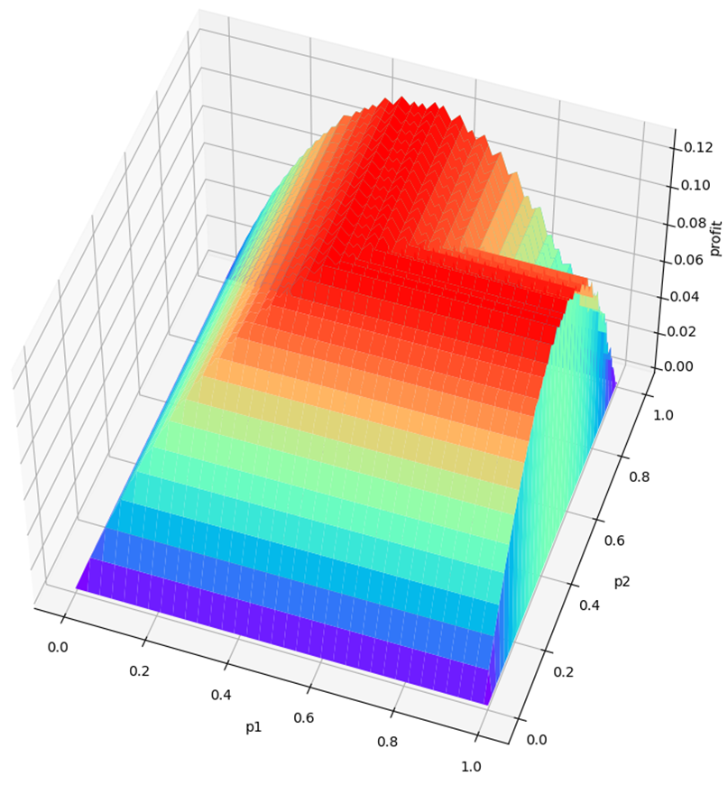
(c) Agent’s maximum profit given $p_{1}$ and $p_{2}$

Figure 2: These pictures show the agent’s strategy.

Panel (a) and Panel (b) of Figure 2 report the agent’s effort $e_{1}$ in project $1$ and $e_{2}$ in project $2$ when two principals choose “tax rate” $p_{1}$ and $p_{2}$. One thing to notice in Figure 2 is that the agent only put the effort in project $1$ when $p_{1}<p_{2}$ and only put the effort in project $2$ when $p_{1}>p_{2}$. This is intuitive since the agent always acts in his best interest and the cost of effort in project $1$ and project $2$ are the same. Therefore, the agent will always choose the project with the lower “tax rate” and the higher expected return.

Panel (c) of Figure 2 reports the agent’s maximum profit given principal $1$’s choice of $p_{1}$ and principal $2$’s choice of $p_{2}$. The agent can achieve this maximum profit if he acts in his best strategy. This strategy would involve the agent making decisions that maximize his expected profit. In this environment, this means putting effort into project $1$ and project $2$ according to the strategy demonstrated in Panel (a) and (b) of Figure 2.

4.4 Principal’s reward function

Two principals choose their own “tax rate” without knowing each other’s choice. Initially, principal $1$’s reward is $(T_{1}-I_{1})e_{1}p_{1}$, and principal $2$’s reward is $(T_{2}-I_{2})e_{2}p_{2}$. But the competition between principal $1$ and principal $2$ will lead them to both choose a “tax rate” close to $0$. And if two principals fully collude with each other, it will be close to the single principal-agent problem. Therefore, we induce a parameter of the rate of “identity of interests” $\beta$. $\beta$ represents how much the two principal’s incentives are aligned with each other. It is a measure of how closely the two principals are working together to achieve a common goal. The higher the $\beta$, the more aligned the two principals’ interests are.

• Principal $1$’s reward is $(T_{1}-I_{1})(e_{1}p_{1}+e_{2}p_{2})\beta+(T_{1}-I_{1})e_{1}p_{1}(1-2\beta)$

• Principal $2$’s reward is $(T_{2}-I_{2})(e_{1}p_{1}+e_{2}p_{2})\beta+(T_{2}-I_{2})e_{2}p_{2}(1-2\beta)$

• $\beta\in[0,0.5]$

4.5 Baseline Parametrization and Initialization

Initially, we focus on a baseline economic environment that consists of a dual contract problem with parameters as follows.

• $I_{1}=I_{2}=1$

• $T=I_{1}+I_{2}=2$

• $c=I_{1}+I_{2}=2$

For this specification, the profit $(T-I)(e_{1}+e_{2})$ is equal to the agent’s cost $\frac{1}{2}c(e_{1}+e_{2})^{2}$ when the agent’s total effort is equal to $1$. This means that when the agent exerts total effort $e1+e2=1$, the net profit will be equal to $0$.

As for the initial matrix $Q_{0}$, our baseline choice is to set the Q-values at $t=0$ at a random number between $0$ and $1$.

The learning parameter $\alpha$ may be in the principal range from $0$ to $1$. we choose $\alpha=0.1$ in our baseline model, following common practice in the computer science literature.

As for the experimentation parameter $\epsilon$, since there is more than one algorithm learning, and if one algorithm experiments more extensively, this creates noise in the environment, which makes it harder for the other to learn. On the other hand, the algorithms need to explore extensively, as the only way to learn is through multiple visits to every state-action cell (of which there are 101 in our baseline experiment with $|S|=1,|A|=101$).

In our baseline model, we use the $\epsilon$-greedy model with a time-declining exploration rate. Specifically, we set

$$\epsilon_{t}=e^{-kt},$$ (4.1)

where $k>0$ is a parameter. This means that initially, the algorithms choose in a purely random fashion, but as time passes, they make the greedy choice more and more frequently. The greater k, the faster the exploration diminishes. Initially, we set $k=5\times 10^{-6}$.

4.6 Pure competition region

When $\beta=0$, two principals seek to maximize the profit from their own project. Because the agent will only put effort into the project with a lower “tax rate”, the competition between the two principals leads them to give a very low “tax rate”, and most of the profit is pocketed by the agent. The outcome of this experiment is reported in Figure 3.

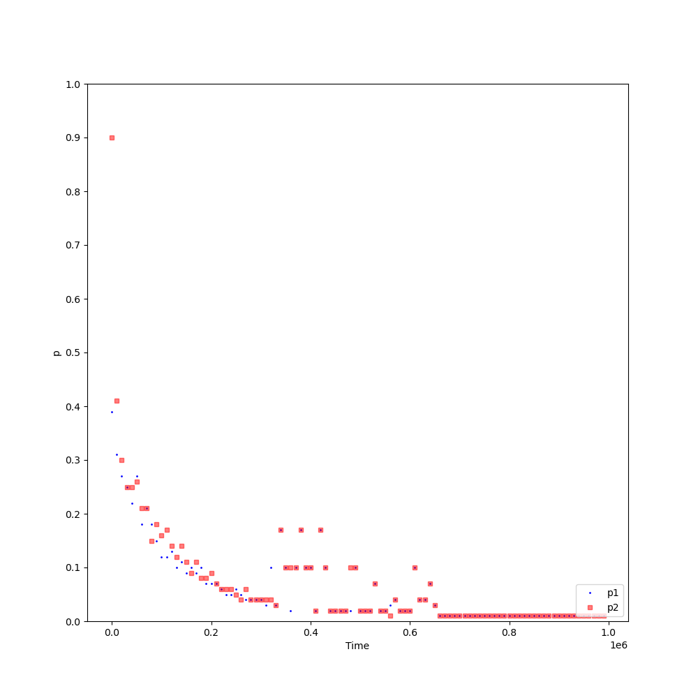
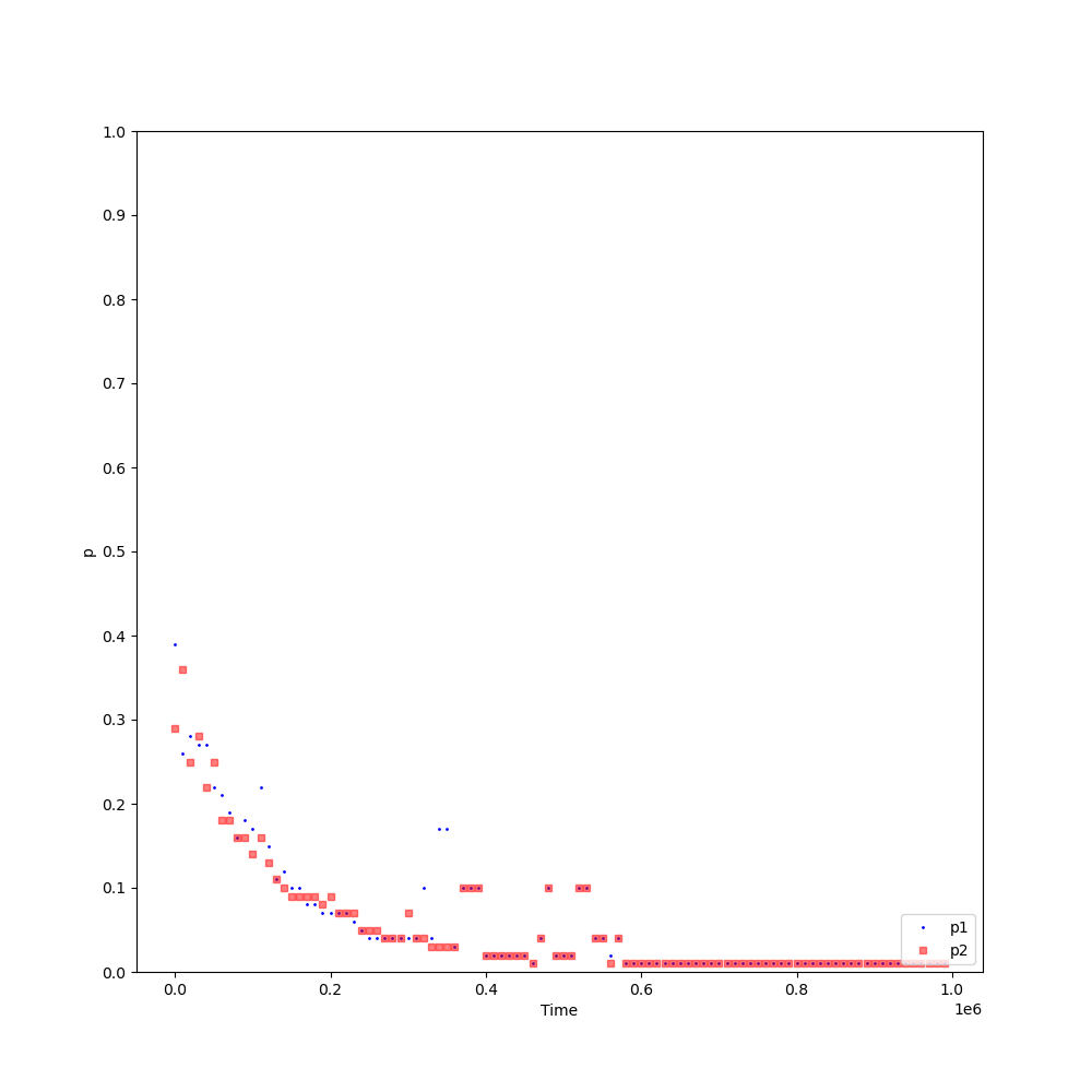
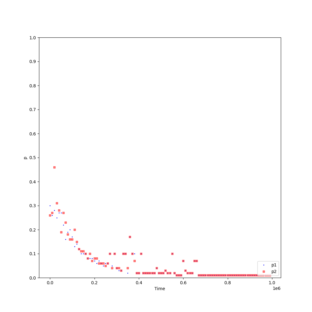
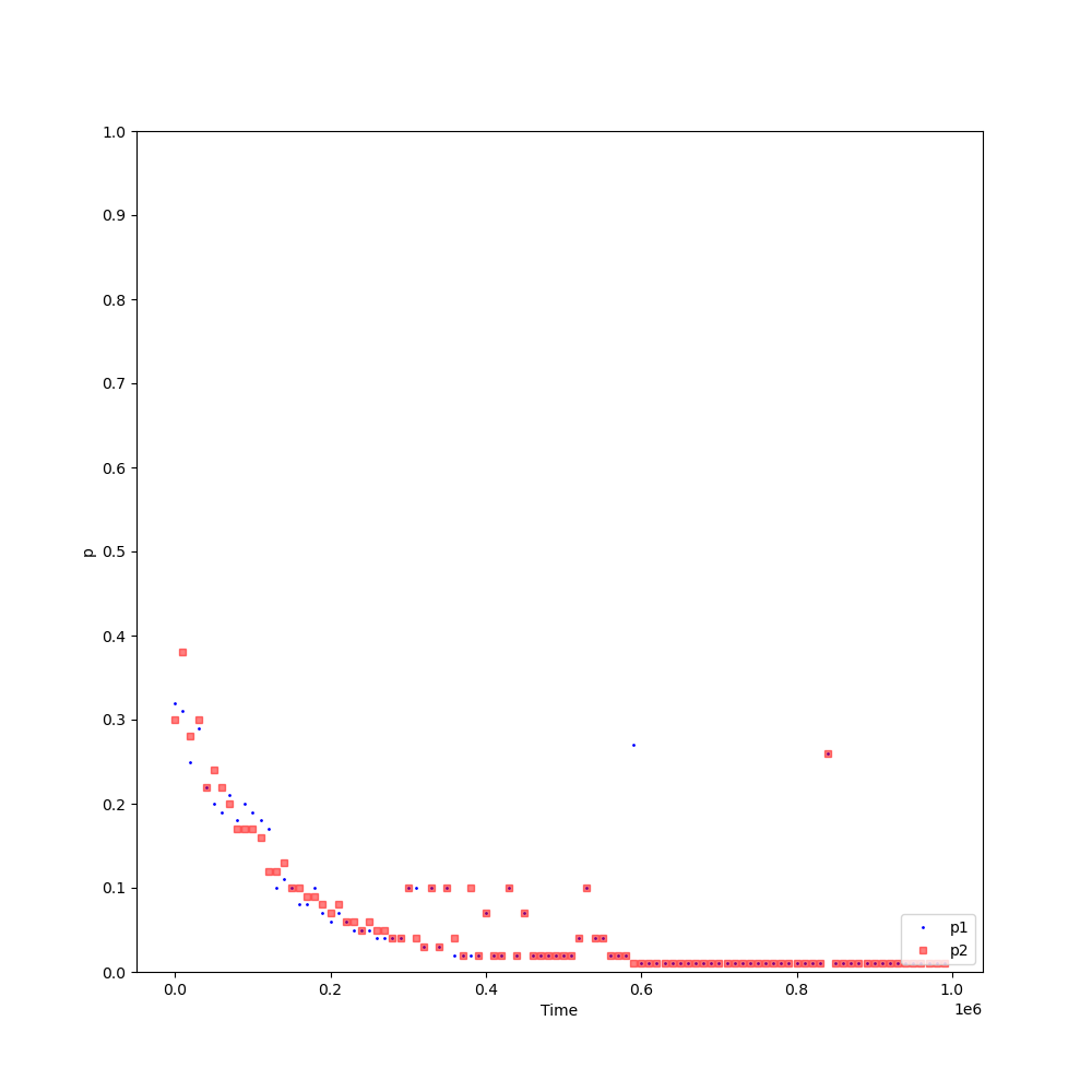
Figure 3: These pictures show the Q-learning algorithms converge to a very low $p$ when $\beta=0$.

Result

Both algorithms converge to the lowest possible positive $p$ ($0.01$ in our case).

In Figure 3, both principal $1$ and principal $2$ converge to the lowest possible positive $p$. This is because if one principal chooses a “tax rate” $p$ higher than the lowest possible positive $p$, then the other principal will try to give a “tax rate” $p$ lower than his competitor. Then the agent will put all his effort into the project provided by the principal with the lower “tax rate”. This will lead to the principal with the higher “tax rate” getting nothing. Because the two principals only consider their own interests, the competition between them forces them to give very low “tax rates”, and both principals cannot get much from their contracts.

4.7 Pure collusion region

When $\beta=0.5$, two principals seek to maximize the profit from both projects. There is no difference between which project the agent puts effort into because two principals will divide the revenue from both contracts evenly. The agent will only put effort into the project with a lower “tax rate”, and only the principal currently giving the lower “tax rate” $p$ can effectively learn during the learning process. Because the agent only does business with the principal with a lower “tax rate”, the principal with a higher “tax rate” cannot gather enough information to effectively update his Q-table. Therefore, when $\beta=0$, the two algorithms seldom converge to the same “tax rate” $p$. The outcome of this experiment is reported in Figure 4.

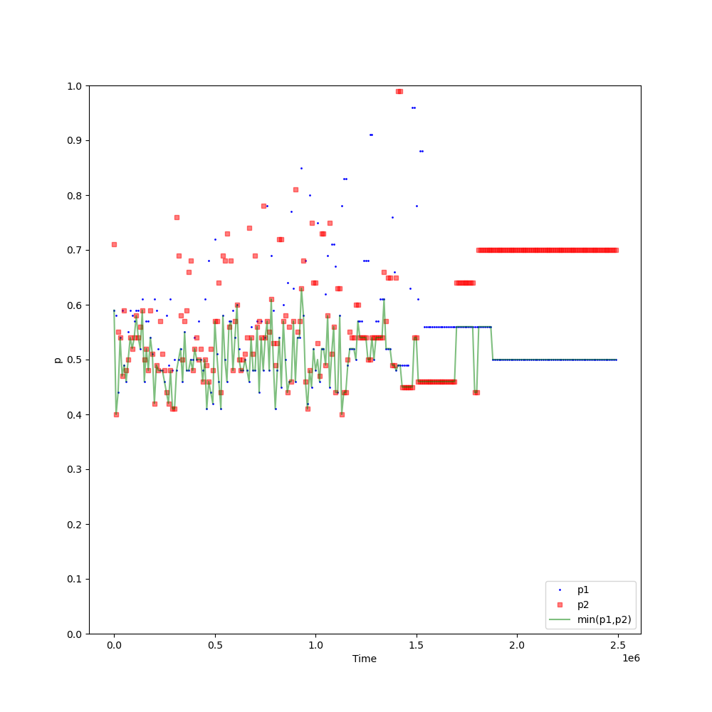
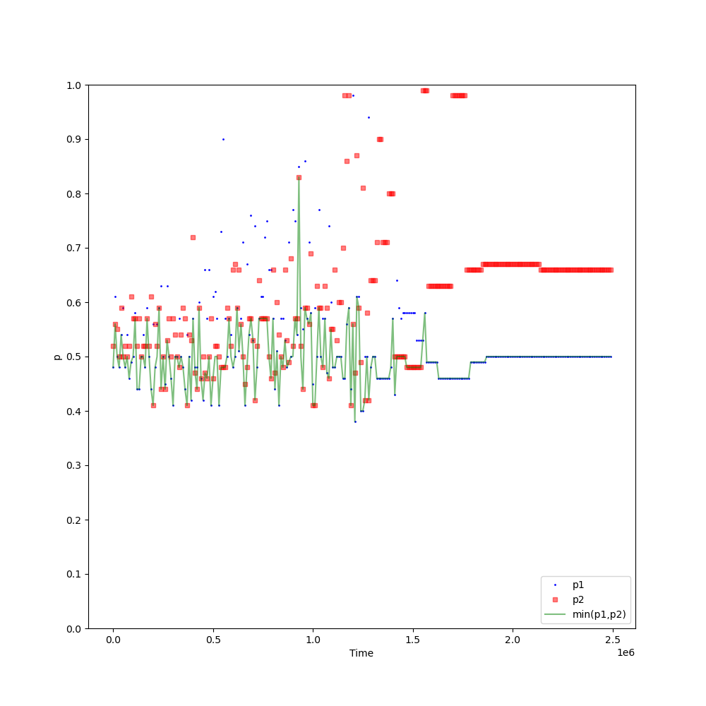
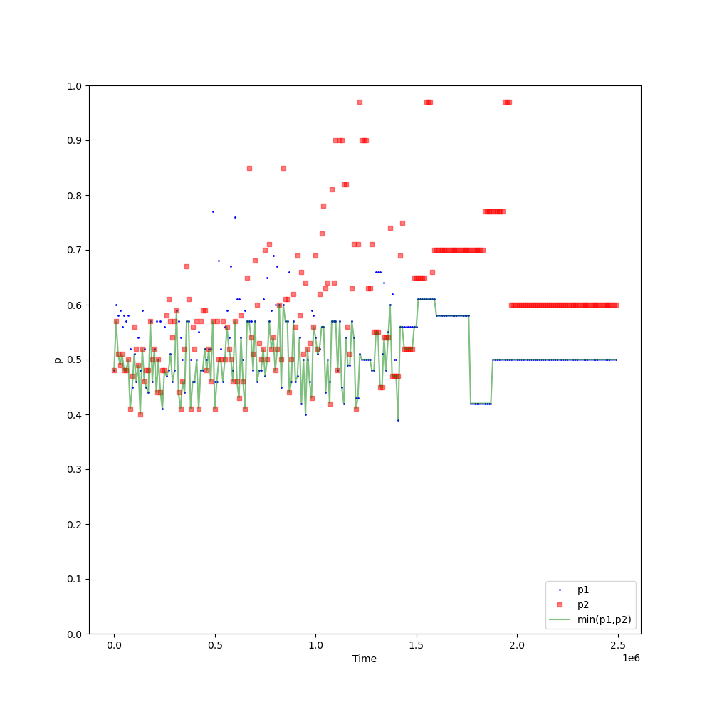
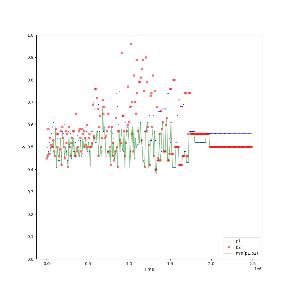
Figure 4: These pictures show the lower “tax rate” two Q-learning algorithms choose converges to the same $p$ ($p=0.5$) as in a single principal-agent problem when $\beta=0.5$.

Result

The lower “tax rate” two Q-learning algorithms choose converges to the same $p$ ($p=0.5$) as in a single principal-agent problem.

In Figure 4, either principal $1$ or principal $2$ converge to the same $p$ ($p=0.5$) as in a single principal-agent problem. This is because the two principals seek to maximize revenues from both contracts. After one principal converges to the optimal “tax rate” $p=0.5$, the other principal who gives a higher $p$ cannot get the information to effectively continue his learning process. So the other principal eventually stays at a “tax rate” higher than the optimal “tax rate”. But we need only focus on the lower “tax rate” two principals choose, as that is what makes an impact on the final revenues the principals and the agent obtain.

One thing to notice in Figure 4 is that the lower “tax rate” the algorithms converge to is higher than the one when $\beta=0$. The total revenue two principals obtain is higher than the one when $\beta=0$. This is intuitive since the principals compete fiercely when $\beta=0$ and the competition between them cuts down their total benefit. When $\beta=0.5$, the interests of the two principals are aligned with each other, so they can reach a certain level of collusion and increase their total benefit.

4.8 Mixed-sum region

When $0<\beta<0.5$, the reward given to each principal is from both his own contract and the other principal’s contract. The bigger the $\beta$, the more the reward is from the other principal’s contract, and the less the reward is from his own contract. When $\beta$ is very low, most of the reward comes from the principal’s own contract. When $\beta$ is high, the reward comes from both principals’ contracts. The outcome is reported in Figure 5.

Result

The greater the $\beta$, the higher the “tax rate” $p$ both principals converge to.

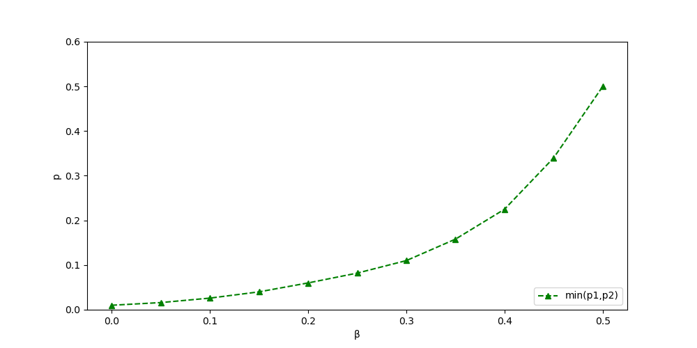
Figure 5: The picture shows the effective “tax rate” two algorithms choose converges to a higher value as $\beta$ grows.

In Figure 5, the “tax rate” $p$ both principals converge to increases as $\beta$ grows. This is because the greater the $\beta$, the more the two principals’ interests are aligned with each other. And the more likely they are to cooperate and work together to raise their “tax rate”. This can lead to a stronger and more successful relationship between the two parties. Aligning interests can also help to reduce conflict and increase the total profit gained by both principals. And the lower the $\beta$, the less two principals’ interests are aligned with each other. This can lead to more competition between the two principals and reduce the total profit gained by both principals.

5 Principal Heterogeneity

In the previous discussion, there is no difference between the two principals. The agent does business with two homogeneous principals. But the agent’s cost of effort in the two principals can be different in the real economy. For example, one principal may be nearer to or have a closer relationship with the agent than the other principal. In this case, the agent may be more willing to do business with the more advantageous principal, given two principals’ “tax rates” are equal. He may be more willing to put effort into the advantageous principal in order to maximize his expected payoff. On the other hand, the agent may be less willing to put effort into the disadvantaged principal if the cost of effort associated with it is higher or the risk associated with it is higher. In this section, we introduce asymmetry in the two principals.

Specifically, we set the agent’s cost of effort

$$cost=\frac{1}{2}c(e_{1}+e_{2})^{2}(1-\kappa+2{\kappa}e_{2}/(e_{1}+e_{2})),e_{1}+e_{2}\neq 0,$$ (5.1)

where $e_{1}{\in}[0,1]$ is the effort the agent put into project $1$, $e_{2}{\in}[0,1]$ is the effort the agent put into project $2$, and $\kappa\in[0,1)$ is a parameter. The agent’s cost is equal to $0$ when $e_{1}+e_{2}=0$. The larger the $\kappa$, the less cost per effort when the agent does business with principal $1$, and the more cost per effort when the agent does business with principal $2$. Therefore, the larger the $\kappa$, the more advantage principal $1$ has over principal $2$. Initially, we set $\kappa=0.2$ in our baseline model.

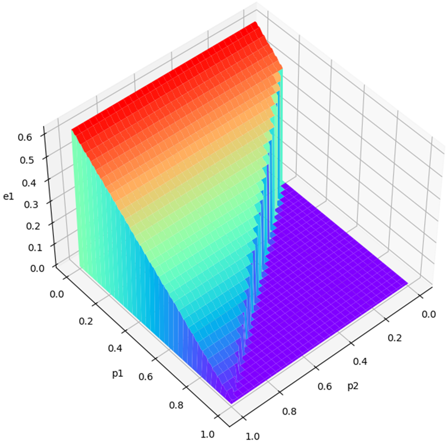
(a) Agent’s effort in project 1

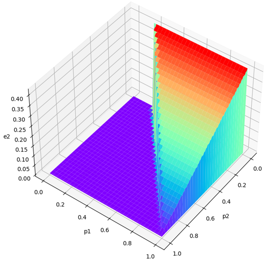
(b) Agent’s effort in project 2

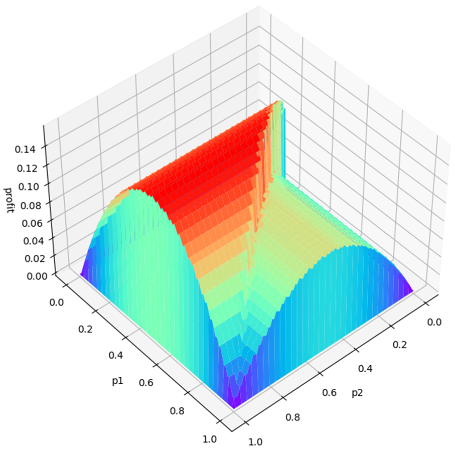
(c) Agent’s maximum profit given $p_{1}$ and $p_{2}$

Figure 6: These pictures show the agent’s strategy in an asymmetric environment.

One thing to notice in Figure 6 (a) and Figure 6 (b) is that compared with the previous symmetric environment, in this asymmetric environment, principal $2$ needs to provide a much lower “tax rate” than his competitor principal $1$ in order to attract the agent to put the effort in his project. And there is an asymmetry in Figure 6 (c). When the agent is doing business with principal $1$, the agent’s profit is significantly higher. This is intuitive since the agent’s cost per effort is lower when in project $1$ and higher in project $2$. The outcome of this experiment is reported in Figure 7.

Result

• Principal $1$ chooses a “tax rate” much higher than $0$ when $\beta=0$.

• The effective “tax rate” $p$ is higher than the one in the symmetric environment ($p=0.5$) when $\beta=0.5$.

• The greater the $\beta$, the higher the effective “tax rate” $p$ (the “tax rate” of the project the agent puts effort into).

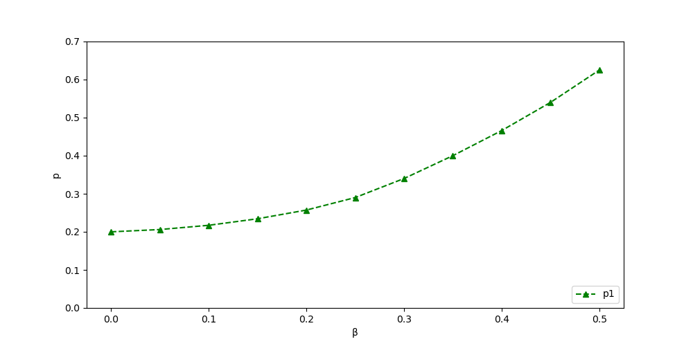
Figure 7: The picture shows the effective “tax rate” two algorithms choose when there is principal heterogeneity.

In Figure 7, the effective “tax rate” ($p_{1}$ in this case) when $\beta=0$ is no longer close to $0$. This is because when there is principal heterogeneity, principal $1$ has an advantage over principal $2$ due to the fact that the agent’s cost per effort is lower when doing business with principal $1$ and higher when doing business with principal $2$. This advantage can, to a certain extent, protect principal $1$ from his competitor, principal $2$. Therefore, principal $1$ can offer a “tax rate” much higher than $0$, increasing his profit without worrying about the competition from principal $2$ when $\beta=0$.

When $\beta=0.5$, two principals seek to maximize the profit from both projects. Now there is no competition because, after all, the two principals divide the revenue from both contracts evenly. Because it is more efficient for the agent to do business with principal $1$, both two principals would like the agent to put effort into project $1$. Thus, the effective “tax rate” is literally the “tax rate” chosen by principal $1$. Because now the agent’s cost per effort is lower, the agent will exert more effort given the same $p$ as in the previous discussion, and principal $1$ is able to raise his “tax rate” and gain more profit. In fact, the effective “tax rate” two Q-learning algorithms choose converges to the same $p$ as in a single principal-agent contract problem with the same parameters.

Similar to the case when there is no principal heterogeneity, the greater the $\beta$, the higher the effective “tax rate” $p$. When $\beta$ is low, two principals compete with each other, and the competition cuts down their total revenue, letting the agent take away most of the projects’ proceeds. The bigger the $\beta$, the more the two principals’ interests are aligned with each other, and their rising level of cooperation will help them raise the effective “tax rate” and get a bigger share from the projects’ proceeds.

6 Conclusion

This paper presents a reinforcement learning approach to autonomously learn incentive compatible contract. We started from our baseline contract model, first showing that the Q-learning algorithm successfully tackle the single principal-agent problem. Then we used multi-agent Q-learning and showed that this method could find the optimal contract in various dual contract problem scenarios. We showed that the algorithms were able to learn an optimal policy and were able to maximize their reward throughout the simulation.

This approach has the potential to be applied to a variety of real-world scenarios, such as the design of incentive contracts or the optimization of resource allocation. Interestingly, many questions remain open. First, one may be worried about the robustness of our findings in allowing other artificial intelligence algorithms to make the contract. We expect that the new methodology we have identified will be present in many algorithms that operate with limited information. Related to that question of other algorithms is what would happen if we made the Q-learning algorithms more sophisticated, for example, by keeping as a state what the opponent’s previous choice was.

Second, we looked at a straightforward environment with definite outcomes for definite actions. One interesting question is how introducing randomness will affect the algorithms finding the optimal contract. Multi-phase contracting and time-varying valuations are also of great interest since they would provide additional insights into using artificial intelligence algorithms that constantly experiment and try to adapt to the changing environment.

Although algorithm contracting may open the way to new forms of best incentive contract mechanism design, it is worth noting that contracting behavior among human decision-makers is more complex. Now we are only focusing on a contract model similar to the debt contract. Whether artificial intelligence algorithms can solve many other contract models remains an open question. It is still unclear how well algorithms can simulate real-life contracting behaviors.

Appendix A Appendix

A.1 Algorithms

Input: Experimentation $\epsilon$, $t_{max}$, principal option dimension $D_{p}$ and learning rate $\alpha$

Output: Learned Q-table $Q$

$t$ = 0; $Q$ = a $1*D_{p}$ array initiated with $Random(0,1)$;

repeat

     

     if (Random(0,1) ¡ $\epsilon$) then

           $Act_{p1}$ = Randint(0, $D_{p}-1$);

          

           else

                $Act_{p1}$ = Argmax($Q$);

               

                end if

               $Act_{a}$ = agentAct($Act_{p1}$);

                $Profit_{p1}$ = calcProfit($Act_{p1}$, $Act_{a}$);

                $Q[Act_{p1}]$ = $(1-\alpha)Q[Act_{p1}]+{\alpha}Profit_{p1}$;

                $t$ ++;

               

                until $t{\geq}t_{max}$;

Algorithm 1 Learning Algorithm in Single Principal-agent Problem

Input: Exploration decay parameter $k$, $t_{max}$, principal option dimension $D_{p}$, learning rate $\alpha$ and $\beta$

Output: Learned Q-tables $Q_{p1}$ and $Q_{p2}$

$t$ = 0; $Q_{p1}$ = a $1*D_{p}$ array initiated with $Random(0,1)$; $Q_{p2}$ = a $1*D_{p}$ array initiated with $Random(0,1)$;

repeat

     

     if (Random(0,1) ¡ $e^{-kt}$) then

           $Act_{p1}$ = Randint(0, $D_{p}-1$);

          

           else

                $Act_{p1}$ = Argmax($Q_{p1}$);

               

                end if

               if (Random(0,1) ¡ $e^{-kt}$) then

                     $Act_{p2}$ = Randint(0, $D_{p}-1$);

                    

                     else

                          $Act_{p2}$ = Argmax($Q_{p2}$);

                         

                          end if

                         $Act_{a}$ = agentAct($Act_{p1}$, $Act_{p2}$);

                          $Profit_{p1}$, $Profit_{p2}$ = calcProfit($Act_{p1}$, $Act_{p2}$, $Act_{a}$);

                          $Q_{p1}[Act_{p1}]$ = $(1-\alpha)Q[Act_{p1}]+{\alpha}({\beta}(Profit_{p1}+Profit_{p2})+(1-2\beta)Profit_{p1})$;

                          $Q_{p2}[Act_{p2}]$ = $(1-\alpha)Q[Act_{p2}]+{\alpha}({\beta}(Profit_{p1}+Profit_{p2})+(1-2\beta)Profit_{p2})$;

                          $t$ ++;

                         

                          until $t{\geq}t_{max}$;

Algorithm 2 Learning Algorithm in Dual Contract Problem

Input: Principal option dimension $D_{p}$, agent option dimension $D_{a}$

Output: Agent choice table $T_{a}$

$V_{a}$ = a $D_{p}*D_{p}*D_{a}$ array initiated with 0;

$T_{a}$ = a $D_{p}*D_{p}$ array initiated with 0;

i,j,k=0;

repeat

      repeat

           repeat

                $Act_{p1}$ = $i{\div}(D_{p}-1)$, $Act_{p2}$ = $j{\div}(D_{p}-1)$, $Act_{a}$ = Decode($k$); $V_{a}[i][j][k]$=agentProfit($Act_{p1}$,$Act_{p2}$,$Act_{a}$);

                $k$ ++;

               

                until $k{\geq}D_{p}$;

               $j$ ++;

               

                until $j{\geq}D_{p}$;

               $i$ ++;

               

                until $i{\geq}D_{p}$;

               i,j=0;

                repeat

                     repeat

                          $T_{a}[i][j]$=Argmax($V_{a}[i][j]$);

                          $j$ ++;

                         

                          until $j{\geq}D_{p}$;

                         $i$ ++;

                         

                          until $i{\geq}D_{p}$;

Algorithm 3 Agent decision algorithm in Dual Contract Problem

References

- Asker et al. (2022) Asker, John, Chaim Fershtman, and Ariel Pakes, 2022, Artificial intelligence, algorithm design, and pricing, AEA Papers and Proceedings 112, 452–56.
- Banchio and Skrzypacz (2022) Banchio, Martino, and Andrzej Skrzypacz, 2022, Artificial intelligence and auction design, in Proceedings of the 23rd ACM Conference on Economics and Computation, 30–31.
- Biais et al. (2007) Biais, Bruno, Thomas Mariotti, Guillaume Plantin, and Jean-Charles Rochet, 2007, Dynamic security design: Convergence to continuous time and asset pricing implications, Review of Economic Studies 74, 345–390.
- Biais et al. (2010) Biais, Bruno, Thomas Mariotti, Jean-Charles Rochet, and Stéphane Villeneuve, 2010, Large risks, limited liability, and dynamic moral hazard, Econometrica 78, 73–118.
- Calvano et al. (2020) Calvano, Emilio, Giacomo Calzolari, Vincenzo Denicolo, and Sergio Pastorello, 2020, Artificial intelligence, algorithmic pricing, and collusion, American Economic Review 110, 3267–97.
- Dai et al. (2020) Dai, Min, Xavier Giroud, Wei Jiang, and Neng Wang, 2020, A q theory of internal capital markets, Technical report, National Bureau of Economic Research.
- DeMarzo and Fishman (2007) DeMarzo, Peter M, and Michael J Fishman, 2007, Optimal long-term financial contracting, Review of Financial Studies 20, 2079–2128.
- DeMarzo et al. (2012) DeMarzo, Peter M, Michael J Fishman, Zhiguo He, and Neng Wang, 2012, Dynamic agency and the q theory of investment, Journal of Finance 67, 2295–2340.
- DeMarzo and Sannikov (2006) DeMarzo, Peter M, and Yuliy Sannikov, 2006, Optimal security design and dynamic capital structure in a continuous-time agency model, The Journal of Finance 61, 2681–2724.
- Edmans et al. (2012) Edmans, Alex, Xavier Gabaix, Tomasz Sadzik, and Yuliy Sannikov, 2012, Dynamic ceo compensation, The Journal of Finance 67, 1603–1647.
- Eloundou et al. (2023) Eloundou, Tyna, Sam Manning, Pamela Mishkin, and Daniel Rock, 2023, Gpts are gpts: An early look at the labor market impact potential of large language models.
- Erev and Roth (1998) Erev, Ido, and Alvin E Roth, 1998, Predicting how people play games: Reinforcement learning in experimental games with unique, mixed strategy equilibria, American economic review 848–881.
- Frydman and Jenter (2010) Frydman, Carola, and Dirk Jenter, 2010, Ceo compensation, Annu. Rev. Financ. Econ. 2, 75–102.
- Gabriel (2020) Gabriel, Iason, 2020, Artificial intelligence, values, and alignment, Minds and machines 30, 411–437.
- Garrett and Pavan (2012) Garrett, Daniel F, and Alessandro Pavan, 2012, Managerial turnover in a changing world, Journal of Political Economy 120, 879–925.
- Garrett and Pavan (2015) Garrett, Daniel F, and Alessandro Pavan, 2015, Dynamic managerial compensation: A variational approach, Journal of Economic Theory 159, 775–818.
- Hadfield-Menell and Hadfield (2019) Hadfield-Menell, Dylan, and Gillian K Hadfield, 2019, Incomplete contracting and ai alignment, in Proceedings of the 2019 AAAI/ACM Conference on AI, Ethics, and Society, 417–422.
- Hansen et al. (2021) Hansen, Karsten T, Kanishka Misra, and Mallesh M Pai, 2021, Frontiers: Algorithmic collusion: Supra-competitive prices via independent algorithms, Marketing Science 40, 1–12.
- He (2009) He, Zhiguo, 2009, Optimal executive compensation when firm size follows geometric brownian motion, The Review of Financial Studies 22, 859–892.
- Innes (1990) Innes, Robert D, 1990, Limited liability and incentive contracting with ex-ante action choices, Journal of economic theory 52, 45–67.
- Kasy and Sautmann (2021) Kasy, Maximilian, and Anja Sautmann, 2021, Adaptive treatment assignment in experiments for policy choice, Econometrica 89, 113–132.
- Kessler and Roth (2012) Kessler, Judd B., and Alvin E. Roth, 2012, Organ allocation policy and the decision to donate, American Economic Review 102, 2018–47.
- Klein (2021) Klein, Timo, 2021, Autonomous algorithmic collusion: Q-learning under sequential pricing, The RAND Journal of Economics 52, 538–558.
- Levin (2003) Levin, Jonathan, 2003, Relational incentive contracts, American Economic Review 93, 835–857.
- Ouyang et al. (2022) Ouyang, Long, Jeff Wu, Xu Jiang, Diogo Almeida, Carroll L Wainwright, Pamela Mishkin, Chong Zhang, Sandhini Agarwal, Katarina Slama, Alex Ray, et al., 2022, Training language models to follow instructions with human feedback, arXiv preprint arXiv:2203.02155 .
- Sannikov (2008) Sannikov, Yuliy, 2008, A continuous-time version of the principal-agent problem, Review of Economic Studies 75, 957–984.
- Scharfstein and Stein (2000) Scharfstein, David S, and Jeremy C Stein, 2000, The dark side of internal capital markets: Divisional rent-seeking and inefficient investment, The journal of finance 55, 2537–2564.
- Schmidt (1997) Schmidt, Klaus M, 1997, Managerial incentives and product market competition, The review of economic studies 64, 191–213.
- Stein (1997) Stein, Jeremy C, 1997, Internal capital markets and the competition for corporate resources, The journal of finance 52, 111–133.
- Watkins and Dayan (1992) Watkins, Christopher JCH, and Peter Dayan, 1992, Q-learning, Machine learning 8, 279–292.
- Zhang et al. (2021) Zhang, Kaiqing, Zhuoran Yang, and Tamer Başar, 2021, Multi-agent reinforcement learning: A selective overview of theories and algorithms, Handbook of reinforcement learning and control 321–384.
- Zhu (2013) Zhu, John Y, 2013, Optimal contracts with shirking, Review of Economic Studies 80, 812–839.
- Zhu (2018) Zhu, John Y, 2018, Myopic agency, The Review of Economic Studies 85, 1352–1388.