Impact of the Hubble tension on the $r-n_{s}$ contour

Abstract

The injection of early dark energy (EDE) before the recombination, a possible resolution of the Hubble tension, will not only shift the scalar spectral index $n_{s}$ towards $n_{s}=1$, but also be likely to tighten the current upper limit on tensor-to-scalar ratio $r$. In this work, with the latest CMB datasets (Planck PR4, ACT, SPT and BICEP/Keck), as well as BAO and SN, we confirm this result, and discuss its implication on inflation. We also show that if we happen to live with EDE, how the different inflation models currently allowed would be distinguished by planned CMB observations, such as CMB-S4 and LiteBIRD.

1 Introduction

Inflation is a current paradigm of the very early universe, predicting a nearly scale-invariant primordial scalar perturbation and primordial gravitational wave (GW). A combined analysis of the CMB observations by Planck with other datasets showed the scalar spectral index $n_{s}=0.965\pm 0.004$ (68% CL) Planck:2018vyg , while its combination with the recent BICEP/Keck dataset showed tensor-to-scalar ratio $r<0.036$ (95% CL) BICEP:2021xfz . However, both results are based on the $\Lambda$CDM model, and cosmological model-dependent.

Recently, some inconsistencies in cosmological observations have been suggested, see e.g. Refs.Perivolaropoulos:2021jda ; Abdalla:2022yfr for recent reviews. The most well-known is the Hubble tension, which have inspired the exploring beyond $\Lambda$CDM model, e.g.DiValentino:2019qzk ; DiValentino:2016hlg ; Mortsell:2018mfj ; Vagnozzi:2019ezj ; Knox:2019rjx ; DiValentino:2019jae ; Schoneberg:2021qvd . In the early dark energy (EDE) resolution Karwal:2016vyq ; Poulin:2018cxd of the Hubble tension, a unknown EDE component before the recombination lowered the sound horizon $r_{s}=\int{c_{s}\over H(z)}dz$ so that $H_{0}$ is lifted, which, however, also brings a unforeseen effect on our understanding on inflation.

It has been found that the injection of EDE will alter the results of $n_{s}$ Ye:2021nej ; Jiang:2022uyg ; Smith:2022hwi ; Jiang:2022qlj , specially if $H_{0}\gtrsim 72$Mpc/km/s, $n_{s}$ will be shifted to $n_{s}=1$ ($|n_{s}-1|\sim{\cal O}(0.001)$)Ye:2020btb , and the current limit on tensor-to-scalar ratio $r$ Ye:2022afu , see also DiValentino:2018zjj ; Giare:2022rvg ; Calderon:2023obf for studies on the possibilities of $n_{s}=1$. Thus some inflation models that had been considered possible in the $\Lambda$CDM model might be excluded, while some inflation models which had been excluded might be reconsidered as possible. However, it is interesting to ask whether the result on $r-n_{s}$ is still credible with the Planck PR4Planck:2020olo , as well as latest ACTACT:2020frw , SPT-3GSPT-3G:2021eoc ; SPT-3G:2022hvq dataset. In this work, we will investigate this issue.

It is expected that cosmological observations would have the ability to discriminate between different inflation models if their precision becomes high enough. In upcoming decade, the Simons ObservatorySimonsObservatory:2018koc , CMB-S4CMB-S4:2016ple , as well as the LiteBIRD satelliteLiteBIRD:2020khw , will play significant roles in improving the constraint on $r-n_{s}$. The combination of CMB-S4 and LiteBIRD will be able to reach $\sigma(n_{s})\sim 0.005$ and $\sigma(r)<10^{-3}$. Here, we also will show how different inflation models allowed by the present observations can be distinguished by upcoming CMB-S4 and LiteBIRD experiments.

The outline of paper is as follows. We show in section 2 the impact of EDE on the current constraint on $r-n_{s}$ and its implication for inflation. The abilities of CMB-S4 and LiteBIRD with EDE is forecasted in section 3. We conclude in section 4. In Appendix A, we present the results with the tensor spectral index $n_{t}$ and running of scalar spectral index $\alpha_{s}$.

2 Results with current data

2.1 Datasets and models

Datasets are as follows:

• PR4: The latest release of Planck maps (PR4), with the NPIPE code Planck:2020olo . We take use of the hillipop likelihood Couchot:2016vaq for high-$\ell$ part and lollipop Tristram:2020wbi as low-$\ell$ polarization likelihood. As for the low-$\ell$ TT power spectrum, we take use of the public commander likelihood Planck:2019nip . Planck PR4 lensing likelihood Carron:2022eyg is included.

• ACT: The ACTPol Data Release 4 (DR4) ACT:2020frw likelihood for all TT, TE, EE power spectrum, which has already been marginalized over SZ and foreground emission.

• SPT: The SPT-3G Y1 data SPT-3G:2021eoc of the TE, EE power spectrum and the recent TT power spectrum data SPT-3G:2022hvq . We take use of the likelihoods adapted for cobaya.

• BK18: The latest BICEP/Keck likelihood on the BB power spectrumBICEP:2021xfz .

• BAO: The 6dF Galaxy Survey Beutler:2011hx and SDSS DR7 main Galaxy sample Ross:2014qpa for the low-$z$ part. The eBOSS DR16 data eBOSS:2020yzd , which include LRG, ELG, Quasar, Ly$\alpha$ auto-correlation and Ly$\alpha$-Quasar cross-correlation, for the high-$z$ part. We use a combined likelihood with the BOSS DR12 BAO data BOSS:2016wmc .

• SN: The uncalibrated measurement of Pantheon+ on the Type Ia supernovae (SNe Ia) ranging in redshift from $z=0.001$ to 2.26. Brout:2022vxf

In this work, for the CMB observations, we consider the combination of Planck and BICEP/Keck, and also the combination of Planck, ACT, SPT and BICEP/Keck (with a cutoff of the PR4 TT spectrum to $\ell$<1000). Besides, we cut the hillipop EE likelihood to $\ell>150$ in order to avoid the correlations with the lollipop likelihood. BAO and SN, which do not conflict with the CMB observations, are included in all datasets.

The injection of EDE before recombination resulted in a lower sound horizon $r^{*}_{\text{s}}$, so a higher $H_{0}$, as $\theta^{*}_{\text{s}}=r^{*}_{\text{s}}/D^{*}_{A}\sim r^{*}_{\text{s}}H_{0}$ is set precisely by CMB observations. The requirement that EDE must decay fast enough to avoid disruption of the CMB fit has motivated different EDE models. Here, we consider the axion-like EDE Poulin:2018cxd , which is achieved by a scale field with axion-like potential (see recent McDonough:2022pku ; Cicoli:2023qri for models in string theory), and the AdS-EDE Ye:2020btb ; Ye:2020oix ; Jiang:2021bab , in which the potential is $\phi^{4}$-like but with an anti-de Sitter phase Ye:2020btb ,

The MCMC sampling is performed using Cobaya Torrado:2020dgo , while we use the modified CLASS Blas:2011rf to calculate models. In addition to the six standard $\Lambda$CDM parameters $\{H_{0},n_{s},\omega_{b},\omega_{\text{cdm}},\tau_{\text{reio}},A_{s}\}$ and $r={A_{T}\over A_{s}}$ at the pivot scale 0.05 Mpc^-1, we also sample on the redshift $z_{c}$ when the field starts rolling and the energy fraction $f_{\text{EDE}}$ at $z_{c}$.

2.2 Results

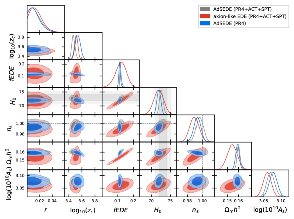
Figure 1: Marginalized posterior distributions (68% and 95% confidence intervals) for relevant parameters in different EDE models with different datasets. BK18 is included in all datasets. Constraint of R21 on $H_{0}$ is shown as a gray band.

parameters	AdSEDE (PR4+ACT+SPT)	axion-like EDE (PR4+ACT+SPT)	AdSEDE (PR4)
$\log_{10}(z_{c})$	$3.470(3.4647)^{+0.022}_{-0.027}$	$3.514(3.5022)\pm 0.044$	$3.540(3.5097)^{+0.035}_{-0.041}$
$f_{\text{EDE}}$	$0.1193(0.11326)^{+0.0028}_{-0.0070}$	$0.119(0.0967)^{+0.038}_{-0.032}$	$0.1123(0.1129)^{+0.0040}_{-0.0062}$
$\Theta_{\text{ini}}$		$2.737(2.752)\pm 0.087$
$r$	$<0.0303$	$<0.0324$	$<0.0284$
$\log(10^{10}A_{\mathrm{s}})$	$3.070(3.0663)\pm 0.011$	$3.060(3.0613)\pm 0.012$	$3.078(3.0763)\pm 0.011$
$n_{\mathrm{s}}$	$0.9966(0.99438)\pm 0.0049$	$0.9893(0.9857)\pm 0.0063$	$0.9932(0.99168)^{+0.0049}_{-0.0044}$
$H_{0}$	$72.62(72.255)^{+0.42}_{-0.51}$	$71.9(71.12)\pm 1.3$	$71.96(71.94)\pm 0.50$
$\Omega_{\mathrm{b}}h^{2}$	$0.02300(0.022928)\pm 0.00016$	$0.02251(0.022424)^{+0.00015}_{-0.00017}$	$0.02321(0.023155)^{+0.00018}_{-0.00016}$
$\Omega_{\mathrm{c}}h^{2}$	$0.1365(0.13588)^{+0.0013}_{-0.0016}$	$0.1319(0.12895)\pm 0.0045$	$0.1352(0.13619)\pm 0.0018$
$\tau_{\mathrm{reio}}$	$0.0521(0.0505)\pm 0.0060$	$0.0542(0.0561)\pm 0.0056$	$0.0591(0.0578)\pm 0.0063$
$\Omega_{\mathrm{m}}$	$0.3038(0.30541)\pm 0.0050$	$0.2987(0.29929)\pm 0.0050$	$0.3072(0.3091)\pm 0.0053$
$S_{8}$	$0.868(0.8676)\pm 0.010$	$0.848(0.8448)\pm 0.012$	$0.871(0.8759)\pm 0.011$

Table 1: 68% confidence intervals for the parameters in different EDE models with different datasets, the best-fit values are shown in parentheses. And for the one-tailed distribution we show 95% confidence intervals. BK18 is included in all datasets.

Our results are shown in Figure 1 and Table 1. In such EDE-like models , we have $H_{0}\gtrsim 72$km/s/Mpc, compatible with the recent local $H_{0}$ measurement Riess:2021jrx (hereafter R21), see also Refs.LaPosta:2021pgm ; Smith:2022hwi ; Jiang:2022uyg with Planck PR3, and Appendix A for the results with $n_{t}$ and the running $\alpha_{s}$ of $n_{s}$.

Apart from the uplift of $H_{0}$, another dramatic change is the shift of the $n_{s}$-$r$ contour, which is shown in Figure 2, specially $n_{s}$ is shifted close to $n_{s}=1$ . The shift of $n_{s}$ is a common result of any prerecombination resolution (without modifying the recombination physics) for the Hubble tension Ye:2021nej . The shift of $n_{s}$ with respect to $H_{0}$ can be approximated as Ye:2021nej ; Jiang:2022uyg :

$$\delta n_{s}\approx 0.4\frac{\delta H_{0}}{H_{0}}.$$ (1)

The upper limit of $r$ (e.g. $r<0.028$ in AdS-EDE) has been slightly lower than that under the $\Lambda$CDM mode $r<0.330$ (PR4) and $r<0.0352$ (PR4+ACT+SPT) This is mainly because the slight uplifts of $\omega_{m}$ and $A_{s}$ in EDE models, compared with $\Lambda$CDM, enhance the lensing spectrum between $200<\ell<800$, while a larger lensing spectrum would imply a smaller $r$ Ye:2022afu .

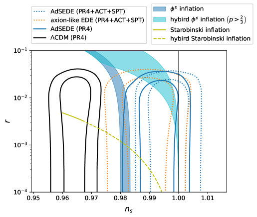
Figure 2: The $r$-$n_{s}$ contour for different models and different combinations of datasets. We also plot the predictions of some inflation models on $n_{s}$ and $r$. The yellow line and the blue band represent Starobinski inflation Starobinsky:1980te and $\phi^{p}$ inflation, respectively, with $50\leqslant N_{*}\leqslant 60$. The dashed yellow line and the cyan band correspond to their hybrid variants where the inflation ended in a deep slow-roll region so that $N_{*}\gg 60$. The left bound ($p=2/3$) of the cyan band is associated with the monodromy inflation Silverstein:2008sg ; McAllister:2008hb and the right bound ($p\rightarrow\infty$) is associated with the power-law inflation Abbott:1984fp .

In well-known single field slow-roll inflation models, $n_{s}$ follows Mukhanov:2013tua ; Kallosh:2013hoa ; Roest:2013fha ; Martin:2013tda

$$n_{s}-1=-{{\cal O}(1)\over N_{*}}$$ (2)

in large $N_{*}$ limit, where ($M_{p}=1$)

$$N_{*}\approx\Delta N+\int_{\phi_{e}}^{\phi_{c}}{d\phi\over\sqrt{2\epsilon}}=\left(\int_{\phi_{c}}^{\phi_{*}}+\int_{\phi_{e}}^{\phi_{c}}\right){d\phi\over\sqrt{2\epsilon}}\approx N(\phi_{*}).$$ (3)

is set by $\phi_{*}$ (at which the perturbation mode with $k=k_{*}$ exits horizon). Thus both $n_{s}$ and $r$ are related to $N_{*}$ rather than $\Delta N$. It is usually thought that the inflation ended at $\phi_{e}$ when the slow-roll condition breaks down, we have $N_{*}=\Delta N\approx 60$ (inflation ends around $\sim 10^{15}\text{GeV}$). However, if inflation ended prematurely at $\phi_{c}$ during the slow-roll regime when $\epsilon\ll 1$, we will have $N_{*}\gg 60$ but still $\Delta N\approx 60$ Kallosh:2022ggf ; Ye:2022efx .

It is interestingly found that some inflation models, such as the power-law inflation Abbott:1984fp and the $\phi^{p}$ inflation Linde:1983gd ; Silverstein:2008sg ; McAllister:2008hb ; Kaloper:2008fb , which were disfavored in the $\Lambda$CDM model, are now compatible with the EDE, see Figure 2. In such inflation models, the inflation might end up by a waterfall instability, which is similar to the hybrid inflation Linde:1991km ; Linde:1993cn , at a deep slow-roll region $\epsilon\ll 1$, so that $N_{*}\gg 60$. The perturbation modes near $N_{*}$ can be just at CMB band, so we have $|n_{s}-1|\ll{\cal O}(0.01)$.

3 Forecast with CMB-S4 and LiteBIRD

It is also significant to investigate the impact of EDE on the constraining power of CMB-S4 and LiteBIRD. The CMB-S4 Abazajian:2019eic will cover the sky area of $f_{\text{sky}}=0.4$, so $20<\ell<5000$ for CMB, while the LiteBIRD LiteBIRD:2020khw is a satellite covering a larger sky area. Here, we assume $f_{\text{sky}}=0.9$ (so $2<\ell<200$) for LiteBIRD, and also set $\ell_{\text{min}}=200$ for CMB-S4 to avoid the correlation between them. And relevant noise power spectrum and delensing are presented in Appendix B.

We use the Fisher matrix to make predictions. The Fisher matrix is the expectation of the Hessian of the log-likelihood:

$$F_{ij}=\left\langle H_{ij}\right\rangle=\left\langle\frac{\partial^{2}\ln\mathcal{L}}{\partial\theta_{i}\partial\theta_{j}}\right\rangle=\operatorname{Tr}\left\{\frac{2\ell+1}{2}f_{\text{sky}}\frac{\partial\mathbf{C}}{\partial\theta_{i}}\mathbf{C}^{-1}\frac{\partial\mathbf{C}}{\partial\theta_{j}}\mathbf{C}^{-1}\right\}$$ (4)

where $\mathbf{C}^{XY}\equiv C_{\ell}^{XY}+N_{\ell}\delta^{XY}$ and $X,Y$ represent T, E, B, respectively. Thus we can estimate the parameter probability covariance matrix: $\mathcal{C}=\mathcal{F}^{-1}$.

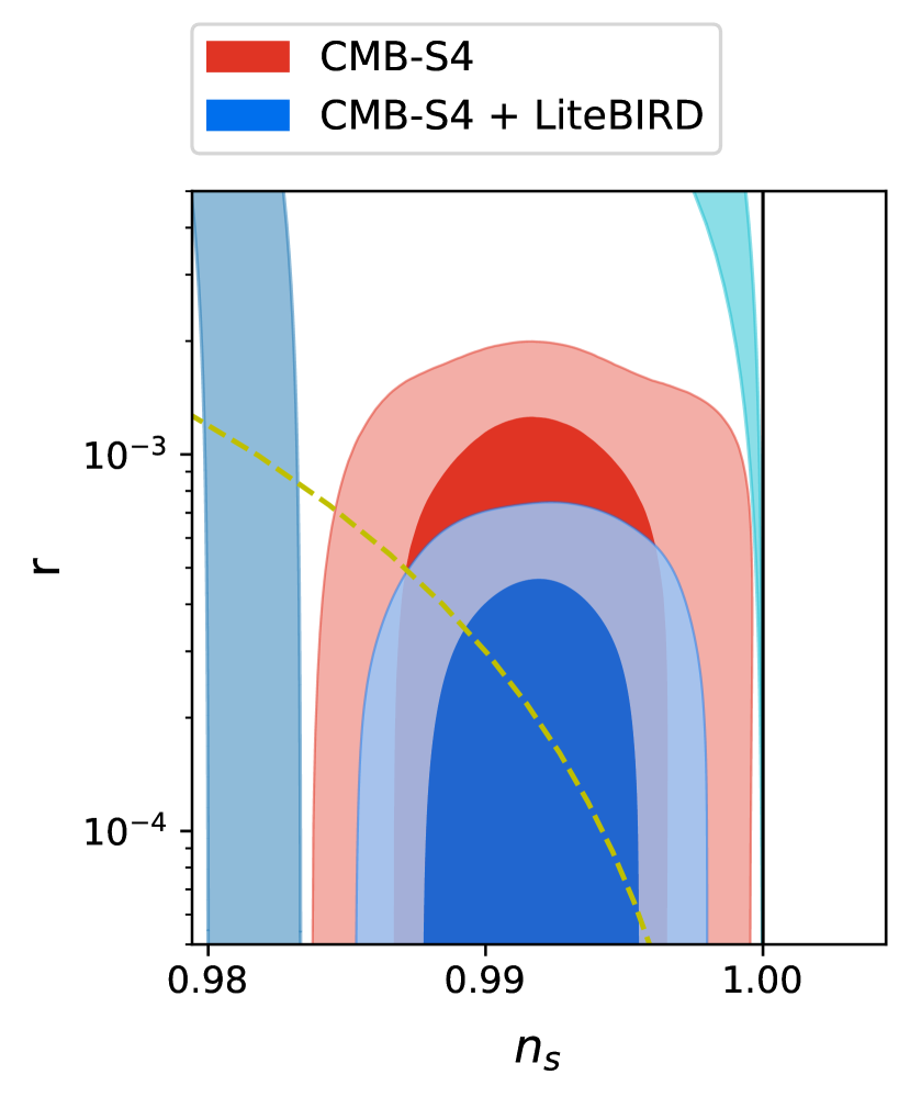
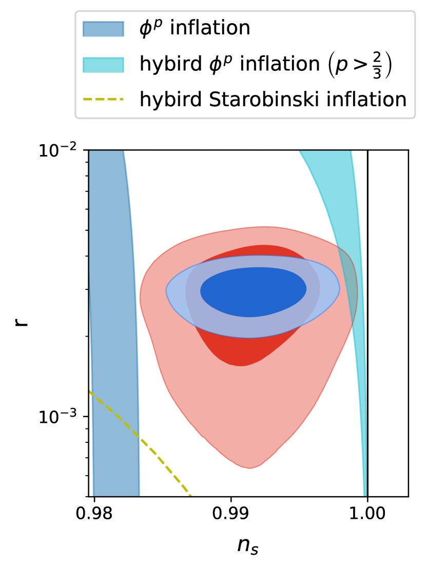
Figure 3: The forecasted $r$-$n_{s}$ contours with CMB-S4 and CMB S4+LiteBIRD in AdSEDE. Based on the bestfit results of AdSEDE for PR4+BK18, we fix $r$ to 0 (left) and 0.003 (right). We also plot the predictions of some inflation models on $n_{s}$ and $r$, the same as Figure 2.

Based on the bestfit results of AdS-EDE for PR4+BK18, we fix $r$ to 0 and 0.003. The results are shown in Figure 3. The $\phi^{p}$ inflation ($p>2/3$) and the power-law inflation with a hybrid end will be ruled out at $2\sigma$ level, if $r$ is still undetected, while the Starobinski inflation with $N_{*}\thickapprox 300$ is consistent, since

$$r={12\over N_{*}^{2}}\sim{\cal O}(1/10^{4}).$$ (5)

However, if $r=0.003$, which would be detected by CMB-S4 and LiteBIRD, the $\phi^{p}$ inflation ($p>2/3$), power-law inflation and Starobinski inflation all will be ruled out at $2\sigma$ level, only the $\phi^{p}$ inflation with $p<2/3$ with a hybrid end might survive.

4 Conclusion

It has been widely thought that the conflicts in cosmological observations imply modifications beyond $\Lambda$CDM model. However, such modifications, specially the injection of EDE before the recombination, might be bringing a unforeseen impact on searching for primordial GW and setting the value of $n_{s}$, so our perspective on inflation.

Here, with the latest CMB datasets, we found for EDE that $|n_{s}-1|\lesssim{\cal O}(0.01)$, while the upper limit of $r$ is also slightly tighten, $r<0.028$ with Planck PR4+BK18 and $r<0.030$ with Planck PR4+ACT+SPT+BK18 dataset, which is consistent with the results with Planck PR3+BK18 Ye:2022afu . In light of our constraint on $r-n_{s}$, the inflation models allowed by the results in the $\Lambda$CDM model, such as Starobinski inflation, will be excluded. However, in corresponding models satisfying (2), if inflation ends by a waterfall instability when inflaton is still at a deep slow-roll region, $n_{s}$ can be lifted close to $n_{s}=1$, so that the inflation models which have been ruled out, such as the $\phi^{p}$ inflation, and also the Starobinski model become possible again with their hybrid variants. It is also interesting to explore other models with $|n_{s}-1|\lesssim{\cal O}(0.01)$.

In upcoming decade, the combination of the CMB-S4CMB-S4:2016ple and the LiteBIRD satelliteLiteBIRD:2020khw will be able to reach $\sigma(n_{s})\sim 0.005$ and $\sigma(r)<10^{-3}$. Here, we also show that the different inflation models allowed by the present observations (if we happen to live with EDE) would be distinguished by both experiments.

Though our analysis considers only the Hubble tension, the inconsistencies in other cosmological observations are also likely to cause the shift of $r-n_{s}$ contour, so impact our perspective on the inflation models. It is possible that the $r-n_{s}$ contour in Figure 2 is not essentially affected, e.g.Ye:2022afu ; Ye:2021iwa . However, relevant issue is still worth questing.

Appendix A Results for $n_{t}$ and $\alpha_{s}$

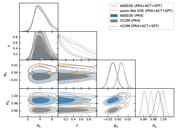
Figure 4: Marginalized posterior distributions (68% and 95% confidence intervals) for relevant parameters under different models and datasets. BK18 is included from all the dataset.

In Figure 4, we present the result for the spectral tilt $n_{t}$ of primordial GW and the running of scalar spectral index $\alpha_{s}=\mathrm{d}n_{s}/\mathrm{d}k$. We imposed the flat priors on both $n_{t}$ and $\alpha_{s}$. We did not find the significant effects of EDE on the observations of $n_{t}$ and $\alpha_{s}$. The main difference on $\alpha_{s}$ is attributed to the different combination of CMB datasets.

However, when we switch from ($r_{\text{pivot}},n_{t}$) to ($r_{k_{1}},r_{k_{2}}$) through

$$r_{k}=r_{\text{pivot}}\left(\frac{k}{k_{\text{pivot}}}\right)^{n_{t}-n_{s}+1}$$ (6)

with $k_{1}=0.002$Mpc^-1 and $k_{1}=0.02$Mpc^-1, in light of Planck18 Planck:2018jri . We find their discrepancy on $r_{2}$, as shown in Figure 5, which is constrained to $r_{2}<0.0457$ and $r_{2}<0.0566$ (95% CL) for AdSEDE and axion-like EDE, respectively, with the PR4+ACT+SPT CMB dataset while $r_{2}<0.0424$ (95% CL) for AdSEDE with the PR4 CMB dataset. Their values are lower than $r_{2}<0.0653$ (95% CL) for $\Lambda$CDM with the PR4 CMB dataset and $r_{2}<0.0656$ (95% CL) with the PR4+ACT+SPT CMB dataset. These discrepancy is more significant than that of $r_{\text{pivot}}$. The main reason is that in EDE the lensing spectrum at this scale ($\ell\sim 250$) is larger Ye:2022afu .

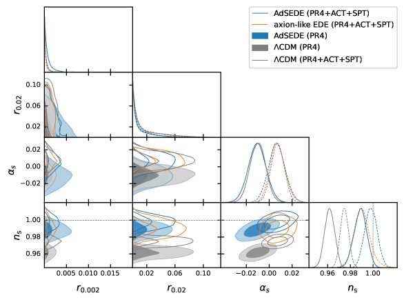
Figure 5: Marginalized posterior distributions (68% and 95% confidence intervals) for relevant parameters under different models and datasets. BK18 is included from all the dataset.

Appendix B On noise power spectrum and delensing

In section 3 we investigate the impact of EDE on the constraining power of CMB-S4 and LiteBIRD. The noise power spectrum $N_{\ell}$ for CMB-S4 is taken from the wiki of CMB-S4. And for LiteBIRD, we consider a noise curve of

$$N_{\ell}^{XY}=s^{2}\exp\left(\ell(\ell+1)\frac{\theta_{\text{FWHM}}^{2}}{8\log 2}\right),$$ (7)

where the temperature noise is $s=2\mu$K-arcmin, $\theta_{\text{FWHM}}=30$ arcmin for the full-width half-maximum beam size LiteBIRD:2022cnt , and the polarization noise has additional factor $\sqrt{2}$.

Delensing on the CMB maps can help improve constraints on $r$ as well as reduce the effects of the cosmological models on the lensing, specially the EDE model. We simply model it as

$$C_{\ell}=A_{L}C_{\ell}^{\text{lensed}}+(1-A_{L})C_{\ell}^{\text{unlensed}}$$ (8)

for the $C_{\ell}$ in Equation 4. The delensing efficiency factor $A_{L}=0.27$ is considered for CMB-S4 and $A_{L}=0.57$ for LiteBIRD LiteBIRD:2022cnt . In addition, we model the effects of thermal dust Planck:2014dmk and synchrotron Choi:2015xha for those polarisation noise power spectrums which have not yet taken the foreground into account as

$$A_{\text{dust }}\ell^{-2.42},\quad\quad A_{\text{synch }}\ell^{-2.3},$$ (9)

respectively, where $A_{\text{dust }}$ and $A_{\text{synch }}$ will be regarded as the nuisance parameters and be marginalised away.

References

- (1) Planck Collaboration, N. Aghanim et al., Planck 2018 results. VI. Cosmological parameters, Astron. Astrophys. 641 (2020) A6, [arXiv:1807.06209]. [Erratum: Astron.Astrophys. 652, C4 (2021)].
- (2) BICEP, Keck Collaboration, P. A. R. Ade et al., Improved Constraints on Primordial Gravitational Waves using Planck, WMAP, and BICEP/Keck Observations through the 2018 Observing Season, Phys. Rev. Lett. 127 (2021), no. 15 151301, [arXiv:2110.00483].
- (3) L. Perivolaropoulos and F. Skara, Challenges for CDM: An update, New Astron. Rev. 95 (2022) 101659, [arXiv:2105.05208].
- (4) E. Abdalla et al., Cosmology intertwined: A review of the particle physics, astrophysics, and cosmology associated with the cosmological tensions and anomalies, JHEAp 34 (2022) 49–211, [arXiv:2203.06142].
- (5) E. Di Valentino, A. Melchiorri, and J. Silk, Planck evidence for a closed Universe and a possible crisis for cosmology, Nature Astron. 4 (2019), no. 2 196–203, [arXiv:1911.02087].
- (6) E. Di Valentino, A. Melchiorri, and J. Silk, Reconciling Planck with the local value of in extended parameter space, Phys. Lett. B 761 (2016) 242–246, [arXiv:1606.00634].
- (7) E. Mörtsell and S. Dhawan, Does the Hubble constant tension call for new physics?, JCAP 09 (2018) 025, [arXiv:1801.07260].
- (8) S. Vagnozzi, New physics in light of the tension: An alternative view, Phys. Rev. D 102 (2020), no. 2 023518, [arXiv:1907.07569].
- (9) L. Knox and M. Millea, Hubble constant hunter’s guide, Phys. Rev. D 101 (2020), no. 4 043533, [arXiv:1908.03663].
- (10) E. Di Valentino, A. Melchiorri, O. Mena, and S. Vagnozzi, Nonminimal dark sector physics and cosmological tensions, Phys. Rev. D 101 (2020), no. 6 063502, [arXiv:1910.09853].
- (11) N. Schöneberg, G. Franco Abellán, A. Pérez Sánchez, S. J. Witte, V. Poulin, and J. Lesgourgues, The H0 Olympics: A fair ranking of proposed models, Phys. Rept. 984 (2022) 1–55, [arXiv:2107.10291].
- (12) T. Karwal and M. Kamionkowski, Dark energy at early times, the Hubble parameter, and the string axiverse, Phys. Rev. D 94 (2016), no. 10 103523, [arXiv:1608.01309].
- (13) V. Poulin, T. L. Smith, T. Karwal, and M. Kamionkowski, Early Dark Energy Can Resolve The Hubble Tension, Phys. Rev. Lett. 122 (2019), no. 22 221301, [arXiv:1811.04083].
- (14) G. Ye, B. Hu, and Y.-S. Piao, Implication of the Hubble tension for the primordial Universe in light of recent cosmological data, Phys. Rev. D 104 (2021), no. 6 063510, [arXiv:2103.09729].
- (15) J.-Q. Jiang and Y.-S. Piao, Toward early dark energy and ns=1 with Planck, ACT, and SPT observations, Phys. Rev. D 105 (2022), no. 10 103514, [arXiv:2202.13379].
- (16) T. L. Smith, M. Lucca, V. Poulin, G. F. Abellan, L. Balkenhol, K. Benabed, S. Galli, and R. Murgia, Hints of early dark energy in Planck, SPT, and ACT data: New physics or systematics?, Phys. Rev. D 106 (2022), no. 4 043526, [arXiv:2202.09379].
- (17) J.-Q. Jiang, G. Ye, and Y.-S. Piao, Return of Harrison-Zeldovich spectrum in light of recent cosmological tensions, arXiv:2210.06125.
- (18) G. Ye and Y.-S. Piao, Is the Hubble tension a hint of AdS phase around recombination?, Phys. Rev. D 101 (2020), no. 8 083507, [arXiv:2001.02451].
- (19) G. Ye and Y.-S. Piao, Improved constraints on primordial gravitational waves in light of the H0 tension and BICEP/Keck data, Phys. Rev. D 106 (2022), no. 4 043536, [arXiv:2202.10055].
- (20) E. Di Valentino, A. Melchiorri, Y. Fantaye, and A. Heavens, Bayesian evidence against the Harrison-Zel’dovich spectrum in tensions with cosmological data sets, Phys. Rev. D 98 (2018), no. 6 063508, [arXiv:1808.09201].
- (21) W. Giarè, F. Renzi, O. Mena, E. Di Valentino, and A. Melchiorri, Is the Harrison-Zel’dovich spectrum coming back? ACT preference for and its discordance with Planck, arXiv:2210.09018.
- (22) R. Calderón, A. Shafieloo, D. K. Hazra, and W. Sohn, On the consistency of CDM with CMB measurements in light of the latest Planck, ACT, and SPT data, arXiv:2302.14300.
- (23) Planck Collaboration, Y. Akrami et al., intermediate results. LVII. Joint Planck LFI and HFI data processing, Astron. Astrophys. 643 (2020) A42, [arXiv:2007.04997].
- (24) ACT Collaboration, S. K. Choi et al., The Atacama Cosmology Telescope: a measurement of the Cosmic Microwave Background power spectra at 98 and 150 GHz, JCAP 12 (2020) 045, [arXiv:2007.07289].
- (25) SPT-3G Collaboration, D. Dutcher et al., Measurements of the E-mode polarization and temperature-E-mode correlation of the CMB from SPT-3G 2018 data, Phys. Rev. D 104 (2021), no. 2 022003, [arXiv:2101.01684].
- (26) SPT-3G Collaboration, L. Balkenhol et al., A Measurement of the CMB Temperature Power Spectrum and Constraints on Cosmology from the SPT-3G 2018 TT/TE/EE Data Set, arXiv:2212.05642.
- (27) Simons Observatory Collaboration, P. Ade et al., The Simons Observatory: Science goals and forecasts, JCAP 02 (2019) 056, [arXiv:1808.07445].
- (28) CMB-S4 Collaboration, K. N. Abazajian et al., CMB-S4 Science Book, First Edition, arXiv:1610.02743.
- (29) LiteBIRD Collaboration, M. Hazumi et al., LiteBIRD: JAXA’s new strategic L-class mission for all-sky surveys of cosmic microwave background polarization, Proc. SPIE Int. Soc. Opt. Eng. 11443 (2020) 114432F, [arXiv:2101.12449].
- (30) F. Couchot, S. Henrot-Versillé, O. Perdereau, S. Plaszczynski, B. Rouillé d’Orfeuil, M. Spinelli, and M. Tristram, Cosmology with the cosmic microwave background temperature-polarization correlation, Astron. Astrophys. 602 (2017) A41, [arXiv:1609.09730].
- (31) M. Tristram et al., Planck constraints on the tensor-to-scalar ratio, Astron. Astrophys. 647 (2021) A128, [arXiv:2010.01139].
- (32) Planck Collaboration, N. Aghanim et al., Planck 2018 results. V. CMB power spectra and likelihoods, Astron. Astrophys. 641 (2020) A5, [arXiv:1907.12875].
- (33) J. Carron, M. Mirmelstein, and A. Lewis, CMB lensing from Planck PR4 maps, JCAP 09 (2022) 039, [arXiv:2206.07773].
- (34) F. Beutler, C. Blake, M. Colless, D. H. Jones, L. Staveley-Smith, L. Campbell, Q. Parker, W. Saunders, and F. Watson, The 6dF Galaxy Survey: Baryon Acoustic Oscillations and the Local Hubble Constant, Mon. Not. Roy. Astron. Soc. 416 (2011) 3017–3032, [arXiv:1106.3366].
- (35) A. J. Ross, L. Samushia, C. Howlett, W. J. Percival, A. Burden, and M. Manera, The clustering of the SDSS DR7 main Galaxy sample – I. A 4 per cent distance measure at , Mon. Not. Roy. Astron. Soc. 449 (2015), no. 1 835–847, [arXiv:1409.3242].
- (36) eBOSS Collaboration, S. Alam et al., Completed SDSS-IV extended Baryon Oscillation Spectroscopic Survey: Cosmological implications from two decades of spectroscopic surveys at the Apache Point Observatory, Phys. Rev. D 103 (2021), no. 8 083533, [arXiv:2007.08991].
- (37) BOSS Collaboration, S. Alam et al., The clustering of galaxies in the completed SDSS-III Baryon Oscillation Spectroscopic Survey: cosmological analysis of the DR12 galaxy sample, Mon. Not. Roy. Astron. Soc. 470 (2017), no. 3 2617–2652, [arXiv:1607.03155].
- (38) D. Brout et al., The Pantheon+ Analysis: Cosmological Constraints, Astrophys. J. 938 (2022), no. 2 110, [arXiv:2202.04077].
- (39) E. McDonough and M. Scalisi, Towards Early Dark Energy in String Theory, arXiv:2209.00011.
- (40) M. Cicoli, M. Licheri, R. Mahanta, E. McDonough, F. G. Pedro, and M. Scalisi, Early Dark Energy in Type IIB String Theory, arXiv:2303.03414.
- (41) G. Ye and Y.-S. Piao, censorship of early dark energy and AdS vacua, Phys. Rev. D 102 (2020), no. 8 083523, [arXiv:2008.10832].
- (42) J.-Q. Jiang and Y.-S. Piao, Testing AdS early dark energy with Planck, SPTpol, and LSS data, Phys. Rev. D 104 (2021), no. 10 103524, [arXiv:2107.07128].
- (43) J. Torrado and A. Lewis, Cobaya: Code for Bayesian Analysis of hierarchical physical models, JCAP 05 (2021) 057, [arXiv:2005.05290].
- (44) D. Blas, J. Lesgourgues, and T. Tram, The Cosmic Linear Anisotropy Solving System (CLASS) II: Approximation schemes, JCAP 07 (2011) 034, [arXiv:1104.2933].
- (45) A. G. Riess et al., A Comprehensive Measurement of the Local Value of the Hubble Constant with 1 km s-1 Mpc-1 Uncertainty from the Hubble Space Telescope and the SH0ES Team, Astrophys. J. Lett. 934 (2022), no. 1 L7, [arXiv:2112.04510].
- (46) A. La Posta, T. Louis, X. Garrido, and J. C. Hill, Constraints on prerecombination early dark energy from SPT-3G public data, Phys. Rev. D 105 (2022), no. 8 083519, [arXiv:2112.10754].
- (47) M. Tristram et al., Improved limits on the tensor-to-scalar ratio using BICEP and Planck data, Phys. Rev. D 105 (2022), no. 8 083524, [arXiv:2112.07961].
- (48) A. A. Starobinsky, A New Type of Isotropic Cosmological Models Without Singularity, Phys. Lett. B 91 (1980) 99–102.
- (49) E. Silverstein and A. Westphal, Monodromy in the CMB: Gravity Waves and String Inflation, Phys. Rev. D 78 (2008) 106003, [arXiv:0803.3085].
- (50) L. McAllister, E. Silverstein, and A. Westphal, Gravity Waves and Linear Inflation from Axion Monodromy, Phys. Rev. D 82 (2010) 046003, [arXiv:0808.0706].
- (51) L. F. Abbott and M. B. Wise, Constraints on Generalized Inflationary Cosmologies, Nucl. Phys. B 244 (1984) 541–548.
- (52) V. Mukhanov, Quantum Cosmological Perturbations: Predictions and Observations, Eur. Phys. J. C 73 (2013) 2486, [arXiv:1303.3925].
- (53) R. Kallosh and A. Linde, Universality Class in Conformal Inflation, JCAP 07 (2013) 002, [arXiv:1306.5220].
- (54) D. Roest, Universality classes of inflation, JCAP 01 (2014) 007, [arXiv:1309.1285].
- (55) J. Martin, C. Ringeval, and V. Vennin, Encyclopædia Inflationaris, Phys. Dark Univ. 5-6 (2014) 75–235, [arXiv:1303.3787].
- (56) R. Kallosh and A. Linde, Hybrid cosmological attractors, Phys. Rev. D 106 (2022), no. 2 023522, [arXiv:2204.02425].
- (57) G. Ye, J.-Q. Jiang, and Y.-S. Piao, Toward inflation with ns=1 in light of the Hubble tension and implications for primordial gravitational waves, Phys. Rev. D 106 (2022), no. 10 103528, [arXiv:2205.02478].
- (58) A. D. Linde, Chaotic Inflation, Phys. Lett. B 129 (1983) 177–181.
- (59) N. Kaloper and L. Sorbo, A Natural Framework for Chaotic Inflation, Phys. Rev. Lett. 102 (2009) 121301, [arXiv:0811.1989].
- (60) A. D. Linde, Axions in inflationary cosmology, Phys. Lett. B 259 (1991) 38–47.
- (61) A. D. Linde, Hybrid inflation, Phys. Rev. D 49 (1994) 748–754, [astro-ph/9307002].
- (62) K. Abazajian et al., CMB-S4 Science Case, Reference Design, and Project Plan, arXiv:1907.04473.
- (63) G. Ye, J. Zhang, and Y.-S. Piao, Alleviating both H0 and S8 tensions: Early dark energy lifts the CMB-lockdown on ultralight axion, Phys. Lett. B 839 (2023) 137770, [arXiv:2107.13391].
- (64) Planck Collaboration, Y. Akrami et al., Planck 2018 results. X. Constraints on inflation, Astron. Astrophys. 641 (2020) A10, [arXiv:1807.06211].
- (65) LiteBIRD Collaboration, E. Allys et al., Probing Cosmic Inflation with the LiteBIRD Cosmic Microwave Background Polarization Survey, arXiv:2202.02773.
- (66) Planck Collaboration, R. Adam et al., Planck intermediate results. XXX. The angular power spectrum of polarized dust emission at intermediate and high Galactic latitudes, Astron. Astrophys. 586 (2016) A133, [arXiv:1409.5738].
- (67) S. K. Choi and L. A. Page, Polarized galactic synchrotron and dust emission and their correlation, JCAP 12 (2015) 020, [arXiv:1509.05934].