EasyDGL: Encode, Train and Interpret for Continuous-time Dynamic Graph Learning

Abstract

Dynamic graphs arise in various real-world applications, and it is often welcomed to model the dynamics directly in continuous time domain for its flexibility. This paper aims to design an easy-to-use pipeline (termed as EasyDGL which is also due to its implementation by DGL toolkit) composed of three key modules with both strong fitting ability and interpretability. Specifically the proposed pipeline which involves encoding, training and interpreting: i) a temporal point process (TPP) modulated attention architecture to endow the continuous-time resolution with the coupled spatiotemporal dynamics of the observed graph with edge-addition events; ii) a principled loss composed of task-agnostic TPP posterior maximization based on observed events on the graph, and a task-aware loss with a masking strategy over dynamic graph, where the covered tasks include dynamic link prediction, dynamic node classification and node traffic forecasting; iii) interpretation of the model outputs (e.g., representations and predictions) with scalable perturbation-based quantitative analysis in the graph Fourier domain, which could more comprehensively reflect the behavior of the learned model. Extensive experimental results on public benchmarks show the superior performance of our EasyDGL for time-conditioned predictive tasks, and in particular demonstrate that EasyDGL can effectively quantify the predictive power of frequency content that a model learn from the evolving graph data.

1 Introduction

1.1 Background and Challenges

Dynamic graph representation learning (DGRL) in general aims to obtain node vector embedding over time $t$ (ideally in continuous time domain, i.e., $t\!\in\!\mathbb{R}$) on graph of which the topological structures and the node attributes are evolving as shown in Fig. 1. Under such a general paradigm, tailored models are often devised and trained according to specific (time-conditioned) predictive tasks, ranging from (dynamic) node classification, link prediction to traffic flow forecasting. These tasks have found widespread application in social networks, bioinformatics, transport, etc.

In practise, a general DGRL pipeline should consist of the encoding framework of which inputs include the graph information and the observed events, learning scheme with the derived loss according to specific tasks at hand. Besides, interpretation of model outputs (e.g., model predictions) is often of high interest in real-world applications. Our following discussion further elaborates on these three aspects.

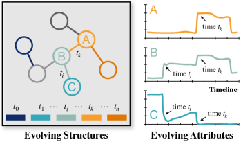
Figure 1: Example of dynamic graph where time $t_{i}$ corresponds to an event of adding edge $(B,C)$. It shows this event changes the graph structures and the node attributes: the connection between node $B$ and node $C$ is changed and the attribute value of node $C$ (in blue) drops significantly. Also, the attribute of node $C$ shows stable trend before the addition of edge $(B,C)$ at time $t_{i}$, then exhibits upward trend until the event of edge $(A,B)$ emerging at time $t_{k}$. This suggests that the structural and temporal dynamics of the observed graph can be entangled.

Figure 2: EasyDGL (encode-train-interpret) pipeline for continuous-time graph. (a) We present the attention-intensity-attention architecture to encode the graph with its event history into node embeddings, for example $\mathbf{h}^{(t)}_{4;l}$ of node $v_{4}$ which is readout from the $l^{\mathrm{th}}$ layer and will be used as input to predict what will happen at a given time $t$ in future. In this example, there are four events of edge addition occurred at time $t_{0},t_{1},t_{2},t_{3}$ respectively. The TPP intensity function is adopted to model the dynamics of events which is then used to modulate attention networks on graph (see Sec. 3). Specifically, the attention (gray colored) encodes endogenous dynamics within neighborhood into $\mathbf{s}^{(t)}_{4;l}$, then it will be coupled with exogenous temporal dynamics by the intensities $\lambda^{\ast}_{k_{1}}(t),\lambda^{\ast}_{k_{2}}(t),\lambda^{\ast}_{k_{3}}(t)$ (blue colored) that specify the occurrence of events on edges $(v_{1},v_{4}),(v_{2},v_{4}),(v_{3},v_{4})$ at time $t$. This quantity that captures evolution of the graph can be used to modulate message passing of the attention (green colored); (b) We consider three popular tasks: dynamic link prediction (see Sec. 4.2.2), dynamic node classification (see Sec. 4.2.3) and node traffic forecasting (see Sec. 4.2.4) under a unified masking-based training scheme; (c) Finally, perturbation-based analysis is performed to quantify the importance of frequency content that the model learns from the data (see Sec. 5) in a scalable way. In particular, it enables model-level interpretation instead of instance-level interpretation as done in most existing explainable graph learning works [16, 48, 67, 66].

$\blacksquare$ Q1: how to efficiently and effectively encode the entangled structural and temporal dynamics of the observed graph?

Earlier works, e.g., DCRNN​[37], DySAT​[51] and STGCN​[63], often view the dynamic temporal graph as a sequence of snapshots with discrete time slots. To improve the model expressiveness and flexibility, continuous-time approaches are recently fast developed whereby the evolution of graph structures and node attributes as shown in Fig. 1 are directly modeled. Beyond the works[33, 45, 61, 35] that encode time into embeddings independent of spatial information, the seminal works[72, 57, 71] explore the use of temporal point process (TPP) techniques for DGRL and introduce the MessagePassing-Intensity framework to capture the entangled spatiotemporal dynamics. Although these approaches have shown promising results, they encounter the common limitations: 1) the message-passing module takes node features as input, whereas the intensity module delivers edge intensity as output. This mismatch between the input and the output limits the MessagePassing-Intensity networks to be used as basic building block that can be stacked to learn high-level features in multi-layered architectures. 2) these works focus on link prediction tasks, as the TPP intensity naturally specifies the occurrence of edge-addition events at any given time. Meanwhile, it is not easy to design intensity based loss for node regression tasks, e.g., traffic forecasting.

With the immense success of attention networks, recent work[10] designs an Attention-Attention framework where the former attention models periodic patterns and the latter attention encodes the structural and temporal dependencies. However, we argue that the lack of the ability to model the evolving patterns in continuous time domain will hurt the performance. CADN[9] develops an ODERNN-Attention encoding framework where ODERNN, an extension of RNN with ordinary differential equation (ODE) solver, is adopted to learn continuous-time dynamics. However, RNN requires sequential computation and thus suffers from slow training. In this paper, we address the aforementioned issues by formalizing an attention-intensity-attention encoding framework, suitable for link-level and node-level applications.

$\blacksquare$ Q2: for typical prediction tasks, how to design a principled family of loss functions and training scheme for dynamic graphs?

In recent years, masked autoencoding has found versatile applications thanks to several groundbreaking practices, such as BERT[13] in natural language processing (NLP) and the very recent MAE[24] in computer vision (CV). The loss of masked autoencoding, which recovers masked parts of the input data, is natural and applicable in DGRL. Recent works[54, 26] randomly mask a portion of the graph data by special tokens and learn to predict the removed content. However, we found that applying such masked training to attention networks for (node) traffic forecasting would hurt the performance (see the results in Table I). We conjecture the reason is that different queries at different timestamps that are replaced by special tokens will have the same query embedding, making the ranking of attention weights of the keys shared across these queries. This may induce a global ranking of influential nodes, which makes sense in domains such as recommender systems and social networks where popular products and top influencers dominate the market. However, a node predictive task might emphasize recently formed edges or certain past timestamps. In this paper, we propose a new correlation-adjusted masking (CaM) for task-aware learning, which can help the attention identify and exploit above patterns in predicting node labels, while enjoying the benefits of existing masking in link prediction.

Despite the masking, the other pursuit for loss design is to make sure that the node embeddings learn the dynamics of the observed graph (e.g., the addition of edges in Fig. 1). In literature, temporal smoothness is often considered [70, 69] which suppresses sharp changes over time. However, we argue that this prior can be sometimes too restrictive to real-world scenarios (see Table I) where graph data evolves quickly. In this paper, we address the issue by introducing the TPP likelihood of events (TPPLE) as a principled way of explaining the graph changes in continuous time domain.

TABLE I: RMSE on the META-LA dataset for 15 minutes, 30 minutes and 45 minutes ahead traffic forecasting, where EasyDGL w/ masking randomly replace the nodes with special tokens[26], and EasyDGL w/ temporal smoothness penalizes the $\ell_{2}$-norm distance of vector embeddings of a node at consecutive snapshots[69].

	15 min	30 min	45 min
EasyDGL w/o CaM and TPPLE	5.618	6.628	7.306
EasyDGL w/ masking	5.653	6.654	7.272
EasyDGL w/ CaM	5.562	6.541	7.162
EasyDGL w/ temporal smoothness	5.908	6.634	7.423
EasyDGL w/ TPPLE	5.598	6.584	7.211

$\blacksquare$ Q3: how to analyze and interpret dynamic node representations or model predictions on large scale graphs over time?

Existing works on interpretable GRL often analyze the importance of neighboring nodes’ features to a query node (mostly indicated by the learned attention weights[16] and the gradient-based weights[48]) as well as the importance of the (sub)graph topologies based on the Shapley value[67]. These works are mainly example-specific and explain why a model predicts what it predicts in the graph vertex domain. It often remains unclear that which frequency information the model is exploiting in making predictions. We note that the quantitative analysis in the graph Fourier domain has a distinct advantage since it can provide the model-level explanations with respect to the intrinsic structures of the underlying graph. In general, model-level explanations are high-level and can summarize the main characteristics of the model (see Table VII for example). To achieve this, there exist two main challenges: 1) the graph Fourier transform (GFT)[46] provides a means to map the data (e.g., model predictions and node embeddings) residing on the nodes into the spectrum of frequency components, but it cannot quantify the predictive power of the learned frequency content. For example in Fig. 8, applying GFT shows that dynamic graph model BERT4REC[54] can learn high-frequency information that is not provided by static graph model GSIMC[6], but it is unclear if BERT4REC outperforms GSIMC because of this high-frequency information. 2) GFT requires to perform orthogonalized graph Laplacian decomposition, whose cost is up to $\mathcal{O}(N^{3})$, cubic to the number of nodes $N$ in the graph. Although Nystr$\mathrm{\ddot{o}}$m methods[19] can obtain the linear cost, their results do not fulfill the orthogonality condition (see more discussion in Sec. 5.2.2). In this paper, we address the challenges by proposing appropriate perturbations in the graph Fourier domain, in company with a scalable and orthogonalized graph Laplacian decomposition algorithm.

1.2 Approach Overview and Contributions

In light of such above discussions, we propose EasyDGL, a new encode, train and interpret pipeline for dynamic graph representation learning, of which the goal is to achieve: 1) effective and efficient encoding of the input dynamic graph with its event history; 2) principled loss design accounting for both prediction accuracy and history fitting; 3) scalable (spectral domain) post-analyzing on large dynamic graphs. The holistic overview of EasyDGL is shown in Fig. 2.

This paper is a significant extension (almost new) of the preliminary works[7]. Our contributions are as follows:

1) Attention-Intensity-Attention Encoding (Sec. 3): the former attention parameterizes the TPP intensity function to capture the dynamics of (edge-addition) events occurred at irregular continuous timestamps, while the latter attention is modulated by the TPP intensity function to compute the (continuous) time-conditioned node embedding that can be easily used for both link-level and node-level tasks. We note that our proposed network can be stacked to achieve highly nonlinear spatiotemporal dynamics of the observed graph, different from existing TPP based works[72, 57, 71, 9]. We also address a new challenge: existing attention models interpret the importance of neighboring node’s features to query node by the learned attention weights[28, 10, 9]. However, they do not provide insight into the importance of the observed timestamps. By contrast, the TPP intensity has the ability to explain the excitation and inhibition effects of past timestamps and events on the future (See Fig. 3).

2) Principled Learning (Sec. 4): we introduce a novel correlation-adjusted masking (CaM) strategy which can derive a family of loss functions for different predictive tasks (node classification, link prediction and traffic forecasting). Specifically, we mask a portion of graph nodes at random: different from prior works that replace masked node with special tokens[54, 64, 62, 26], in EasyDGL the masked key nodes are removed and not used for training, which provides diversified topologies of the observed graph in multiple epochs and allows us to process a portion of graph nodes. This can reduce the overall computation and memory cost; masked query nodes are replaced with their labels, which encourages the attention to focus on the keys whose embeddings are highly correlated with the label information of the query. We also add time encodings to every node; without this, masked nodes would have no information about their “locations” in graph. The task-aware loss with masking on dynamic graph is further combined with a task-agnostic loss based on the TPP posterior maximization that accounts for the evolution of a dynamic graph. This term (called TPPLE) replaces the temporal smoothing prior as widely used in existing works[70, 69] that assume no sharp changes.

3) Scalable and Perturbation-based Spectral Interpretation (Sec. 5): to our knowledge, for the first time we achieve $\mathcal{O}(Nsr\!+\!r^{3})$ ($N,s,r$ is the number of graph nodes, sampled columns and Laplacian eigenvectors respectively) complexity to transform model outputs into frequency domain by introducing a scalable and orthogonalized graph Laplacian decomposition algorithm, while vanilla techniques require $\mathcal{O}(N^{3})$ cost. On top of it, we design intra-perturbations and inter-perturbations to perturb model predictions (or node embeddings) in the graph Fourier domain and examine the resulting change in model accuracy to precisely quantify the predictive power of the learned frequency content. Note that the frequency in fact describes the smoothness of outputted predictions with respect to the underlying graph structure, which is more informative than plain features.

4) Empirical Effectiveness (Sec. 6). We evaluate EasyDGL on real-world datasets for traffic forecasting, dynamic link prediction and node classification. Experimental results verify the effectiveness of our devised components, and in particular EasyDGL achieves $6.7\!-\!14.5\%$ relative Hit-Rate gains and $11.4\!-\!14.7\%$ relative NDCG gains over state-of-the-art baselines on challenging Netflix data (with $497,959$ nodes and $100,444,166$ edges). The source code is available at https://github.com/cchao0116/EasyDGL.

2 Background and Problem Statement

We first briefly introduce the basics of attention and temporal point process for dynamic graphs, then formally describe our problem setting and notations, and finally provide further discussion on related works.

2.1 Preliminaries

2.1.1 Graph Attention Networks

Suppose that $v_{u}$ is the query node and a set $\mathcal{N}_{u}$ represents its neighbors of size $|\mathcal{N}_{u}|=n$, then in the general formulation, attention network computes the embedding $\mathbf{h}_{u}$ for query $v_{u}$ as a weighted average of the features $\{\mathbf{v}_{i}\}$ over the neighbors $v_{i}\in\mathcal{N}_{u}$, using the learned attention weights $e_{u,i}$:

$$\begin{split}\mathrm{Att}(\mathbf{h}_{u}|\mathcal{N}_{u},\mathbf{v})&=\sum_{i\in\mathcal{N}_{u}}\left(\frac{\exp(e_{u,i})}{\sum_{i^{\prime}\in\mathcal{N}_{u}}\exp(e_{u,i^{\prime}})}\right)\mathbf{v}_{i}\\ &=\sum_{i\in\mathcal{N}_{u}}Q(\mathbf{v}_{i}|\mathbf{h}_{u})\mathbf{v}_{i}=\mathbf{E}_{\mathbf{v}_{i}\sim{Q}}\mathbf{v}_{i},\end{split}$$ (1)

where $Q(\mathbf{v}_{i}|\mathbf{h}_{u})$ is the normalized attention weight (score) that indicates the importance of node $v_{i}$’s features to node $v_{u}$. It is worth pointing out that the scoring function $e_{u,i}$ can be defined in various ways, and in the literature three popular implementations for representation learning on graphs are self-attention networks (SA) [58], graph attention networks (GAT) [59] and its recent variant GATv2 [5]:

$$\mathrm{SA} :\quad e_{u,i}=\mathbf{q}_{u}^{\top}\mathbf{k}_{i}/\sqrt{d}$$ (2)

$$\mathrm{GAT} :\quad e_{u,i}=\mathrm{LeakyReLU}(\mathbf{a}^{\top}\big{[}\,\mathbf{k}_{u}\parallel\mathbf{k}_{i}\,\big{]})$$ (3)

$$\mathrm{GATv2} :\quad e_{u,i}=\mathbf{a}^{\top}\mathrm{LeakyReLU}(\big{[}\,\mathbf{k}_{u}\parallel\mathbf{k}_{i}\,\big{]})$$ (4)

where $\mathbf{q}_{u}\in\mathbb{R}^{d}$ and $\mathbf{k}_{i}\in\mathbb{R}^{d}$ are the transformed features of query node $v_{u}$ and key node $v_{i}\in\mathcal{N}_{u}$ respectively, $\mathbf{a}\in\mathbb{R}^{2d}$ is the model parameter and $\parallel$ is the concatenation operation.

2.1.2 Temporal Point Process and Intensity Function

Temporal pint process (TPP) is a stochastic model for the time of the next event given all the times of previous events $\mathcal{H}_{t}\!\coloneqq\!\{(k_{i},t_{i})|t_{i}<t\}$, where the tuple $(k_{i},t_{i})$ corresponds to an event of type $k_{i}\in\{1,\dots,K\}$ occurred at time $t_{i}$ and $K$ is the total number of event types. The dynamics of the arrival times can equivalently be represented as a counting process $\mathrm{N}(t)$ that counts the number of events occurred at time $t$. In TPPs, we specify the above dynamics using the conditional intensity function $\lambda_{k}^{\ast}(t)$ that encapsulates the expected number of type-$k$ events occurred in the infinitesimal time interval $[t,t+\mathrm{d}t]$[11] given the history $\mathcal{H}_{t}$:

$$\lambda_{k}^{\ast}(t)\,\mathrm{d}t=\mathbf{E}\Big{[}\mathrm{N}_{k}(\mathrm{d}t\big{|}\mathcal{H}_{t})\Big{]},$$ (5)

where $*$ reminds that the intensity $\lambda^{\ast}$ is history dependent, $\mathrm{N}_{k}(\mathrm{d}t|\mathcal{H}_{t})$ denotes the number of type-$k$ events falling in a time interval $[t,t\!+\!\mathrm{d}t)$. Note that the conditional intensity function has a relation with the conditional density function of the interevent times, according to survival analysis [1]:

$$f_{k}^{\ast}(t)\!=\!\lambda_{k}^{\ast}(t)\exp\Bigg{(}-\int_{t_{n}}^{t}\lambda^{\ast}(s)\,\mathrm{d}s\Bigg{)},\lambda^{\ast}(s)\!=\!\sum_{k=1}^{K}\lambda_{k}^{\ast}(s)$$ (6)

where the exponential term is called the survival function $S^{\ast}(t)$ that characterizes the conditional probability that no event happens during $[t_{n},t)$, and $t_{n}$ is the last event occurred before time $t$. Using the chain rule, the likelihood for a point pattern $\{(t_{i},k_{i})|t_{i}<T)\}$ is given by

$$L=\Bigg{(}\prod_{i=1}^{n}\lambda_{k_{i}}^{\ast}(t_{i})\Bigg{)}\exp\Bigg{(}-\int_{0}^{T}\lambda^{\ast}(s)\,\mathrm{d}s\Bigg{)},$$ (7)

where the integral for all possible non-events is intractable to compute, and we describe two algorithms to approximate the integral in Sec. 4.1.

TABLE II: Summary of existing literature on representation learning for dynamic graphs based on different types of dynamic graph definitions (discrete and continuous-time), encoding architectures, masked training schemes, model interpreting techniques and embedding evolving strategies.

Method	Dynamic Graph	Encoding Architecture	Masked Training	Model Interpreting	Embedding Evolving
DCRNN [37]	Discrete	GCN-RNN	N/A	N/A	Snapshot-based
STGCN [63]	Discrete	GCN-CNN	N/A	N/A	Snapshot-based
DSTAGNN [34]	Discrete	Attention-GCN-CNN	N/A	N/A	Snapshot-based
EvolveGCN [47]	Discrete	GCN-RNN	N/A	N/A	Snapshot-based
GREC [64]	Discrete	Convolution	Special tokens	N/A	Snapshot-based
DySAT [51]	Discrete	Attention	N/A	Attention coefficient	Snapshot-based
BERT4REC [54]	Discrete	Attention	Special tokens	Attention coefficient	Snapshot-based
JODIE [33]	Continuous	GraphSAGE-RNN	N/A	N/A	Event-triggered
TGN [50]	Continuous	MessagePassing-RNN	N/A	N/A	Event-triggered
DyREP [57]	Continuous	MessagePassing-Intensity	N/A	TPP intensity	Spontaneous
TGAT[61]	Continuous	TimeEncoding-Attention	N/A	Attention coefficient	Spontaneous
TiSASREC[35]	Continuous	TimeEncoding-Attention	N/A	Attention coefficient	Spontaneous
CADN [9]	Continuous	ODERNN-Attention	N/A	Attention coefficient	Spontaneous
TimelyREC [10]	Continuous	Attention-Attention	Special tokens	Attention coefficient	Spontaneous
CTSMA∗[7]	Continuous	Attention-Intensity-Attention	N/A	Both of above	Spontaneous
EasyDGL (ours)	Continuous	Attention-Intensity-Attention	CaM & TPPLE	+ Spectral perturbation	Spontaneous

^∗Conference version of this work.

2.2 Problem Formulation and Notations

Definition 1 (Graph).

A directed graph $\mathcal{G}=\{\mathbb{V},\mathbb{E}\}$ contains nodes $\mathbb{V}\!=\!\{v_{1},\dots,v_{N}\}$ and edges $\mathbb{E}\subseteq\mathbb{V}\times\mathbb{V}$, where $(u,v)\in\mathbb{E}$ denotes an edge from a node $u$ to node $v$. An undirected graph can be represented with bidirectional edges.

Definition 2 (Dynamic Graph).

Suppose that $\mathcal{G}$ is a graph representing an initial state of a dynamic graph at time $t_{0}$, let $\mathcal{O}$ denote the set of observations where tuple $(u,v,\mathrm{op}_{t})\!\in\!\mathcal{O}$ denotes an edge operation $\mathrm{op}_{t}$ of either addition or deletion conducting on edge $(u,v)\in\mathbb{E}$ at time $t$, then we represent a continuous-time (dynamic) graph as a pair $(\mathcal{G},\mathcal{O})$, while a discrete-time (dynamic) graph is a set of graph snapshots sampled from the dynamic graph at regularly-spaced times, represented as $\{\mathcal{G}_{0},\mathcal{G}_{1},\dots\}$.

Definition 3 (Continuous-time Representation).

Given a continuous-time graph $(\mathcal{G},\mathcal{O})$, if node $v_{u}$ involves $n$ events at time $\{t_{1},\dots,t_{n}\}$ and $\mathcal{X}\!\!=\!\!\{\mathbf{X}^{(1)},\dots,\mathbf{X}^{(n)}\}$ denotes dynamic node attributes, then we define its continuous-time representation at any future timestamp $t>t_{n}$ by $\mathbf{h}^{(t)}_{u}$:

$$\mathbf{h}^{(t)}_{u}=\text{GRL}(u,t;\mathcal{G},\mathcal{O},\mathcal{X})$$ (8)

where GRL represents graph representation learning model.

Definition 4 (Dynamic Link Prediction).

Given $(\mathcal{G},\mathcal{O})$ and let $v_{u}$ denote the query node, then the goal of dynamic link prediction is to predict which is the most likely vertex that will connect with node $v_{u}$ at a given future time $t$:

$$(\mathcal{G},\mathcal{O},\mathcal{X};u,t)\stackrel{{\scriptstyle\mathbf{h}_{u}^{(t)}}}{{\longrightarrow}}\textit{prob. of $v_{i}$ connecting with $v_{u}$}.$$ (9)

Definition 5 (Dynamic Node Classification).

Given $(\mathcal{G},\mathcal{O})$ and $v_{u}$, then dynamic node classification aims to predict the label $\mathbf{y}^{(t)}_{u}$ of node $v_{u}$ at a given future time $t$:

$$(\mathcal{G},\mathcal{O},\mathcal{X};u,t)\stackrel{{\scriptstyle\mathbf{h}_{u}^{(t)}}}{{\longrightarrow}}\mathbf{y}_{u}^{(t)}.$$ (10)

Definition 6 (Traffic Forecasting).

Given $\mathcal{X}\!=\!\{\mathbf{X}^{(t)}\}$ and $\mathbf{X}^{(t)}\!\in\!\mathbb{R}^{N\times{P}}$ denotes the speed readings at time $t$ where $P$ is the number of features, then existing approaches for traffic forecasting maintain a sliding window of $T^{\prime}$ historical data to predict future $T$ data, on a given road network (graph) $\mathcal{G}$:

$$[\mathbf{X}^{(t-T^{\prime}+1)},\dots,\mathbf{X}^{(t)};\mathcal{G},\mathcal{O}]\longrightarrow[\mathbf{X}^{(t+1)},\dots,\mathbf{X}^{(t+T)}].$$ (11)

To capture the dynamics on graph, in this paper we focus on the events of edge addition and define a temporal point process on dynamic graph:

Definition 7 (TPP on Dynamic Graph and Events of Edge Addition).

Given any query node $v_{u}$ and its neighborhood $\mathcal{N}_{u}$, we introduce the modeling of a TPP on $v_{u}$ where the event is defined as the addition of an edge connecting node $v_{u}$. In such case, the intensity $\lambda_{i}^{\ast}(t)$ essentially models the occurrence of edges between node $v_{i}$ and node $v_{u}$ at time $t$. However, it is expensive to compute $\lambda_{i}^{\ast}(t)$ for all $v_{i}\in\mathcal{N}_{u}$. To address the issue, we propose to first cluster nodes into $K$ groups and make the nodes in the same (for example, $k$-th) group share the intensity $\lambda_{k}^{\ast}(t)$ for reduced computation cost, i.e., from $\mathcal{O}(|\mathcal{N}_{u}|)$ to $\mathcal{O}(K)$.

In Sec. 3, we will show how to adapt the conditional intensity function as defined by Eq. (5) to the fine-grained modeling of a continuous-time graph $(\mathcal{G},\mathcal{O})$. While in Sec. 4 we present our training scheme that uses Eq. (7) to account for the observed events $\mathcal{O}$ of edge addition on graph $\mathcal{G}$.

We note that the dynamic experimental protocol requires the model to predict what will happen at a given future time, and it has already been shown more reasonable for evaluating continuous-time/discrete-time approaches in[29].

2.3 Related Works

In literature, discrete-time dynamic graph approaches have been extensively studied due to ease of implementation. It can be mainly categorized into tensor decomposition[41, 42, 18] and sequential modeling[37, 68, 47, 2, 34, 63, 51] two families. By contrast, continuous-time graph approaches are relatively less studied. In the following, we review the related works in two aspects: 1) spatio-temporal decoupled modeling, where continuous-valued timestamps are directly encoded into vectorized representations; and 2) spatio-temporal entangled modeling, in which the structural information is considered in temporal modeling.

2.3.1 Spatio-temporal Decoupled Modeling Methods

Early works assume that temporal dynamics are independent of structural information in the graph. A line of works[33, 49, 45, 20] adopt temporally decayed function to make recently formed nodes/edges more important than previous ones. Differently, in [35] the elapsed time data is divided into bins, such that continuous-valued timestamps can be embedded into vector representations, analogous to positional encoding. This idea of time encoding is extended by[61, 21] using nonlinear neural networks and sinusoidal functions, respectively. While the assumption of independence is desired for many cases, in some applications the structural and temporal dynamics are entangled.

2.3.2 Spatio-temporal Entangled Modeling Methods

Recent effort has been made to capture the entangled structural and temporal dynamics over graph. In [43, 57, 71], the intensity function of TPP is parameterized with deep (mostly recurrent) neural networks to model spatiotemporal dynamics. These works focus on link prediction tasks and are orthogonal to us as they build task specific methods and do not focus on representation learning. In contrast,​[9, 27] include the ordinary differential equations (ODE) to capture continuous evolution of structural properties coupled with temporal dynamics. Typically, the ODE function is parameterized with an RNN cell and updates hidden states in a sequential manner, not optimal on industrial scale data. [10] proposes a novel Attention-Attention architecture where the former attention captures periodic patterns for each node while the latter attention models the entangled structural and temporal information. Note that this method does not consider continuous-time evolving patterns.

As summarized in Table II, most of existing continuous-time approaches either perform time encoding or deep RNN to model the fine-grained temporal dynamics. By contrast, we propose a TPP-modulated attention network which can efficiently model the entangled spatiotemporal dynamics on industry-scale graph. As mentioned above, one shortcoming of existing masking strategies is that they might not provide satisfactory results for node-level tasks. Our method tackles this problem by designing TPPLE and CaM. Additionally, it is unclear for existing models which frequency content they are exploiting in making their predictions. We propose a perturbation-based spectral graph analyzing technique to provide insight in the graph Fourier domain. Another observation is that in EasyDGL, the embedding for each node is essentially a function of time (spontaneous) which characterizes continuous evolution of node embedding, when no observations have been made on the node and its relations. This addresses the problem of memory staleness[29] that discrete-time and event-triggered approaches suffer.

3 Encoding: Attention-Intensity-Attention
Scheme for Temporal-structural Embedding

In Sec. 3.1, we generalize the attention to continuous time space and discuss the motivation behind our idea. We then present in Sec. 3.2 the detailed architecture that encodes the entangled structural and temporal dynamics on graph.

3.1 Parameterizing Attention in Continuous Time

Suppose that $v_{u}$ is the query node and $\mathcal{H}_{t}$ represents a set of historical events up to time $t$, in order to compute the node representation $\mathbf{h}_{u}^{(t)}$, it is necessary to know if node $v_{u}$ is still connected with node $v_{i}\in\mathcal{N}_{u}$ at a future time $t$. To account for this, we use $\mathrm{N}_{i}(\mathrm{d}t\big{|}\mathcal{H}_{t})\!\in\!\mathbb{N}_{+}$ to denote the number of edges $(v_{i},v_{u})$ appearing within a short time window $[t,t\!+\!\mathrm{d}t)$. For example in social networks, $\mathrm{N}_{i}(\mathrm{d}t\big{|}\mathcal{H}_{t})\!=\!2$ indicates that user $v_{u}$ revisits user $v_{i}$ twice during $[t,t\!+\!\mathrm{d}t)$. With this, we can reformulate the attention in Eq. (1) as:

$$\mathrm{Att}(\mathbf{h}^{(\mathrm{d}t)}_{u}|\mathcal{N}_{u},\mathbf{v})=\mathbf{E}_{\mathbf{v}_{i}\sim{Q}}\mathrm{N}_{i}(\mathrm{d}t\big{|}\mathcal{H}_{t})\mathbf{v}_{i},$$ (12)

where $\mathbf{h}^{(\mathrm{d}t)}_{u}$ denotes node representation during the interval $[t,t\!+\!\mathrm{d}t)$ and the distribution $Q$ corresponds to the normalized attention coefficient in Eq. (1). However, it is intractable to train above attention network in Eq. (12) on large graphs, because the model parameters $\mathrm{N}_{i}(\mathrm{d}t\big{|}\mathcal{H}_{t})$ are restricted to be integers. To relax the integer constraint, one of feasible solutions is to replace the discrete counting number by its continuous relaxation $\mathbf{E}[\mathrm{N}_{i}(\mathrm{d}t\big{|}\mathcal{H}_{t})]$. To that end, we derive the generalized attention as follows:

$$\mathrm{Att}(\mathbf{h}^{(\mathrm{d}t)}_{u}|\mathcal{N}_{u},\mathbf{v}) =\mathbf{E}_{\mathbf{v}_{i}\sim{Q}}\mathbf{E}\Big{[}\mathrm{N}_{i}(\mathrm{d}t\big{|}\mathcal{H}_{t})\Big{]}\mathbf{v}_{i}$$

$$=\mathbf{E}_{\mathbf{v}_{i}\sim{Q}}\lambda_{i}^{\ast}(t)\mathbf{v}_{i}\,\mathrm{d}t,$$ (13)

where Eq. (13) holds due to Eq. (5) where $\lambda_{i}^{\ast}(t)\mathrm{d}t$ specifies the number of type-$i$ events, i.e., new edges on pair $(v_{i},v_{u})$ during $[t,t\!+\!\mathrm{d}t)$. Since we are interested in the embedding $\mathbf{h}_{u}^{(t)}$ at a single point $t$ in the time dimension, we have:

$$\mathrm{Att}(\mathbf{h}^{(t)}_{u}|\mathcal{N}_{u},\mathbf{v})=\mathbf{E}_{\mathbf{v}_{i}\sim{Q}}\lambda_{i}^{\ast}(t)\mathbf{v}_{i}.$$ (14)

3.1.1 Further Discussion

Connections to Existing Attentions. We note that given $\mathcal{N}_{u}$, existing attention [5, 58, 59, 40] will produce identical node embedding $\mathbf{h}^{(t)}_{u}$ for different past timestamps $\{t_{i}\}$ and future timepoint $t$, thereby making attention a static quantity. Essentially, these approaches can be viewed as our special cases with constant $\lambda_{i}^{\ast}(t)\!\equiv\!{1}$ for $v_{i}\in\mathcal{N}_{u}$. In other words, EasyDGL modulates the attention with the TPP intensity so as to energize attention itself a temporally evolving quantity.

Figure 3: TPP-based interpreting of EasyDGL for dynamic link prediction on Netflix, which shows a user’s intensities for different event types (or item clusters defined in Eq. (15)) over time. One can see that this user has consistent interests in movies of type-0 and-1, while the interests in movies from type-5 to type-7 are transient, i.e., $[t_{11},t_{17}]$ in one day.

To clarify our advantages over static attention networks, we conclude three properties with examples from user-item behavior modelling (see Fig. 3 for case studies on Netflix):

1. When $\lambda_{i}^{\ast}(t)\!=\!0$, the impact of neighbor $v_{i}$ is rejected. $\Rightarrow$ The items (e.g., baby gear) purchased far from now may not reflect user’s current interests.

2. When $\lambda_{i}^{\ast}(t)\!<\!1$, the impact of neighbor $v_{i}$ is attenuated. $\Rightarrow$ Buying cookies may temporarily depress the purchases of all desserts.

3. When $\lambda_{i}^{\ast}(t)\!>\!1$, the impact of neighbor $v_{i}$ is amplified. $\Rightarrow$ Buying cookies may temporarily increase the probability of buying a drink.

However, it is challenging to perform our attention on very large graphs, since the conditional intensity $\lambda_{i}^{\ast}(t)$ need to be computed $|\mathcal{N}_{u}|$ times for all $v_{i}\in\mathcal{N}_{u}$. One feasible solution is to cluster the nodes into groups, then we model the dynamics of the observed events at the group level:

$$\mathrm{Att}(\mathbf{h}^{(t)}_{u}|\mathcal{N}_{u},\mathbf{v}) =\mathbf{E}_{\mathbf{v}_{i}\sim{Q}}\lambda_{k_{i}}^{\ast}(t)\mathbf{v}_{i}$$

$$=\sum_{i\in\mathcal{N}_{u}}Q(\mathbf{v}_{i}|\mathbf{h}^{(t)}_{u})\lambda_{k_{i}}^{\ast}(t)\mathbf{v}_{i},$$ (15)

where $k_{i}$ is the cluster identity for node $v_{i}$. The rationale behind this is that the nodes in one group share the dynamic patterns. This makes sense in many domains such as recommender systems where the products of the same genre have similar patterns. Also, this design shares the parameters in each cluster that mitigates data sparsity issue.

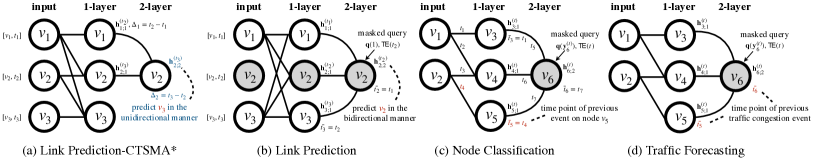
Figure 4: Encoding and training of EasyDGL with three typical dynamic prediction tasks. The left (a) is performed in an auto-regressive manner; while the right three devised in this paper are based on auto-encoding. (a) Our conference work [7] (i.e. CTSMA) tailored for dynamic link prediction; (b) Link prediction (Sec. 4.2.2): given a sequence of user behaviors $\{v_{1},v_{2},v_{3}\}$ on a user-item bipartite graph and $v_{2}$ is randomly selected for being masked, at the $1^{\mathrm{st}}$ layer the time delta as defined in Eq. (19) is set to $t_{1}-t_{0}$, $t_{2}-t_{1}$ and $t_{3}-t_{2}$ respectively, when computing $\mathbf{h}^{(t_{1})}_{1;1},\mathbf{h}^{(t_{2})}_{2;1}$ and $\mathbf{h}^{(t_{3})}_{3;1}$. Note that the output $\mathbf{h}^{(t_{2})}_{2;2}$ at the $2^{\mathrm{nd}}$ layer has direct access to information of all three time intervals with constant path length $\mathcal{O}(1)$, superior to recursive architectures[43, 57]; (c) Node classification (Sec. 4.2.3): Let $v_{6}$ denote the masked query node whose input features are replaced by its true label $\mathbf{y}_{6}^{(t)}$, and the one-hop neighbors $v_{3},v_{4},v_{5}$ are most recently updated at time $t_{1},t_{3},t_{4}$ respectively, then the time intervals are set to $t-t_{1},t-t_{3},t-t_{4}$ when computing $\mathbf{h}_{3;1}^{(t)},\mathbf{h}_{4:1}^{(t)},\mathbf{h}_{5;1}^{(t)}$; (d) Traffic forecasting (Sec. 4.2.4): $v_{6}$ denotes the masked query node whose input features are replaced by its true speed reading $\mathbf{y}_{6}^{(t)}$. Note that $\bar{t}_{5}$ ($\bar{t}_{6}$) represents the time point of previous traffic congestion event occurred on $v_{5}$ ($v_{6}$).

3.2 Instantiating Continuous Time Attention Encoder

We next instantiate the encoding network in EasyDGL as defined in Eq. (15). Let $\mathbf{X}^{f}\!\in\!\mathbb{R}^{N\times{F}}$ and $\mathbf{X}^{c}\!\in\!\mathbb{R}^{N\times{K}}$ denote node feature matrix and cluster assignment matrix, where $N,F,K$ is the number of nodes, features and clusters respectively. $\mathbf{X}^{c}$ is obtained using weighted kernel K-means [14] based on the data $\mathbf{X}^{f}$, and assignments for new nodes can be decided inductively by using cluster centroids.

3.2.1 Overview of the Encoding Network

The encoding network consists of four key steps and follows an attention-intensity-attention scheme:

1. Clustering structure encoding. In real world, nodes might interact with each other at a group level. For example, the purchase of a smart phone will increase the likelihood of buying phone cases. To account for this, a new encoding is added to all nodes in the graph.

2. Endogenous dynamic encoding (Attention). Since the temporal and structural dynamics are entangled in domains like road networks, we propose a specific attention-intensity-attention design. We first employ an attention network to encode localized changes in the neighborhood (i.e., the endogenous dynamics). When an event changes spatial graph structures or node attributes, the representation outputted from the attention will be changed accordingly.

3. Conditional intensity modeling (Intensity). Then we couple the structure-aware endogenous dynamics with the time-dependent exogenous dynamics by devising a new intensity function that specifies the occurrence of events on edges. Note that different input events and different event timestamps will result in different intensities.

4. Intensity-attention modulating (Attention). As the learned intensity naturally offers us the ability to specify the occurrence of edge-addition events at a specific future time, a new attention mechanism is proposed by using the intensity to modulate the attention in Step 2. The resulting attention can yield continuous-time node embeddings.

3.2.2 Clustering Structure Encoding

To capture the group-level interactions, we add “clustering structure encodings” to the input embeddings as an initial step, followed by linear transformation:

$$\mathbf{H}^{(t)}_{0} =\big{[}\,\mathbf{X}^{f}\parallel\mathbf{X}^{c}\,\big{]}$$ (16)

$$\mathbf{V}^{(t)}_{l} =\mathbf{W}^{V}\mathbf{H}^{(t)}_{l-1}$$ (17)

where $\parallel$ is the concatenation operation and $\mathbf{W}^{V}$ is a weight matrix that might be different at different layer $l$; $\mathbf{H}_{l-1}^{(t)}$ and $\mathbf{V}_{l}^{(t)}$ signifies the node representations outputted from layer $l\!-\!1$ and the value representations at layer $l$, respectively.

3.2.3 Endogenous Dynamics Encoding

We next employ deep attention network to capture localized changes in graph structures and node attributes (namely, the endogenous dynamics) within the neighborhood. Let $v_{u}$ denote the query node and set $\mathcal{N}_{u}$ denotes its neighborhood, then we encode such dynamics into representation $\mathbf{s}_{u;l}^{(t)}$:

$$\mathbf{s}_{u;l}^{(t)}=\sum_{i\in\mathcal{N}_{u}}\left(\frac{\exp(e^{(t)}_{u,i})}{\sum_{i^{\prime}\in\mathcal{N}_{u}}\exp(e^{(t)}_{u,i^{\prime}})}\right)\mathbf{v}^{(t)}_{i;l},$$ (18)

where $\mathbf{v}^{(t)}_{i;l}$ is the $i^{\mathrm{th}}$ column of $\mathbf{V}^{(t)}_{l}$, $e^{(t)}_{u,i}$ is the attention coefficient which can be implemented in various ways (e.g., SA[58], GAT [59] and GATv2 [58]). Note that $e^{(t)}_{u,i}$ essentially models the associations between clusters since it implicitly computes the interaction between cluster embeddings, analogous to the positional encoding [58].

3.2.4 Conditional Intensity Modeling

Recall that $\mathcal{H}_{t}\!=\!\{(t_{i},k_{i})|t_{i}<t\}$ denotes the history, where pair $(t_{i},k_{i})$ signifies the occurrence of type-$k_{i}$ event at time $t_{i}$ — a new edge connecting $v_{u}$ and one node in group $k_{i}$ appears in graph at time $t_{i}$. To model the dynamics of events, we combine the structure-aware endogenous dynamics $\mathbf{s}^{(l)}_{u;l}$ with the time-dependent exogenous dynamics:

$$\mathbf{g}^{(t)}_{k;l}=\sigma\Big{(}\underbrace{\mathbf{W}^{G}_{k}\mathbf{s}^{(t)}_{u;l}}_{\text{Endogenous}}+\underbrace{\vphantom{\mathbf{W}^{G}_{k}\mathbf{s}^{(l)}_{u;l}}\mathbf{b}^{G}_{k}(t-\bar{t}_{u})}_{\text{Exogenous}}\Big{)},$$ (19)

where $\mathbf{W}_{k}^{G}\!,\mathbf{b}^{G}_{k}$ are the model parameters for cluster $k$, and $\bar{t}_{u}$ signifies the time point of previous event for $v_{u}$. Fig. 4 provides examples of $\bar{t}_{u}$ in versatile applications.

The intensity $\lambda^{\ast}_{k}(t)$ for type-$k$ event takes the form:

$$\lambda^{\ast}_{k}(t)=f_{k}\left(\mathbf{w}^{\top}_{k}\mathbf{g}^{(t)}_{k;l}+\mu_{k}\right),$$ (20)

where $\mathbf{w}_{k}$ is the parameter for $k^{\mathrm{th}}$ cluster, and $\mu_{k}$ signifies the base occurrence rate. It has been well studied in [57, 71] that the choice of activation function $f_{k}$ should consider two critical criteria: i) the intensity should be non-negative and ii) the dynamics for different event types evolve at different scales. To account for this, we adopt the softplus function:

$$f_{k}(x)=\phi_{k}\log({1}+\exp(x/\phi_{k})),$$ (21)

where the parameter $\phi_{k}$ captures the timescale difference.

One may raise concerns regarding Eq. (19) that it might lose information by looking only at time point of previous event $\bar{t}_{u}$. We argue that as shown in Fig. 4, the maximum path length between any two recent time points is $\mathcal{O}(1)$ in multi-layered architectures, superior to $\mathcal{O}(|\mathcal{N}_{u}|)$ for typical neural TPP models[43, 57].

3.2.5 Intensity-Attention Modulating

We use TPP intensity to modulate the attention following Eq. (15):

$$\mathbf{h}_{u;l}^{\mathrm{(t)}}=\sum_{i\in\mathcal{N}_{u}}\left(\frac{\exp(e^{(t)}_{u,i})}{\sum_{i^{\prime}\in\mathcal{N}_{u}}\exp(e^{(t)}_{u,i^{\prime}})}\right)\lambda^{\ast}_{k_{i}}(t)\mathbf{v}_{i;l}^{(t)},$$ (22)

where $\mathbf{h}_{u;l}^{\mathrm{(t)}}$ is in fact the $u^{\mathrm{th}}$ column of $\mathbf{H}^{(t)}_{l}$ that will be used as input of next layer to derive $\mathbf{H}^{(t)}_{l+1}$, and $k_{i}$ is the cluster index of neighbor $v_{i}$. In practise, using multi-head attention is beneficial to increase model flexibility. To facilitate this, we compute $\mathbf{h}_{u;l}^{\mathrm{(t)}}$ with $H$-independent heads:

$$\mathbf{h}_{u;l}^{\mathrm{(t)}}=\bigg{\Arrowvert}_{h=1}^{H}\mathbf{h}_{u;l;h}^{\mathrm{(t)}},$$ (23)

where $\mathbf{h}_{u;l;h}^{\mathrm{(t)}}$ is computed using different set of parameters.

4 Training: Task-agnostic Posterior Maximization and Task-aware Masked Learning

We consider a principled learning scheme which consists of both task-agnostic loss based on posterior maximization that accounts for the whole event history on dynamic graph, as well as task-aware loss under the masking-based supervised learning. We note that the task-agnostic loss can be viewed as a regularizer term in addition to the discriminative supervised term for applications, ranging from link prediction, node classification and traffic forecasting.

4.1 TPP Posterior Maximization of Events on Dynamic Graphs for Task-aware Learning

Among existing solutions, temporal smoothness[70, 69] penalizes the distance between consecutive embeddings for every node to prevent sharp changes. However, this might not be desired in some applications such as recommender systems where a user’s preference will change substantially from one time to another. To address the issue, we propose to maximize the TPP likelihood of events $\mathcal{H}_{t}$ (TPPLE) that encourages the embeddings to learn evolving dynamics.

Let $\mathbf{y}$ denote the ground-truth label, $\hat{\mathbf{y}}_{\Theta}$ represents the predicted result where $\Theta$ denotes model parameters, and function $\ell(\mathbf{y},\hat{\mathbf{y}}_{\Theta})$ measures the difference between the label and the prediction. Then, we optimize $\Theta$ by minimizing the following risk:

$$\min_{\Theta}\mathbf{E}_{\mathbf{y}}\ell(\mathbf{y},\hat{\mathbf{y}}_{\Theta})-\gamma\mathbf{E}_{u}\,R(\Theta;u),$$ (24)

where $\gamma$ is a hyper-parameter which controls the strength of the regularization; $R(\Theta;u)$ signifies our TPPLE term which maximizes the log-likelihood of the whole observed events $\{(k_{1},t_{1}),\dots,(k_{n},t_{n})\}$ for any given query node $v_{u}$:

$${R}(\Theta;u)=\sum_{i=1}^{n}\log\lambda^{\ast}_{k_{i}}(t_{i})-\int_{t_{0}}^{t_{n}}\lambda^{\ast}(s)\,\mathrm{d}s$$ (25)

where recall that $\lambda^{\ast}(s)=\sum_{k}\lambda_{k}^{\ast}(s)$ is the conditional intensity for the entire history sequence. As stated in Sec. 2.1.2, we recall that the sum term in the right hand side represents the log-likelihood of all the observations, while the integral term represents the log-survival probability that no event happens during the time window $[t_{0},t_{n})$.

However, it is rather challenging to compute the integral $\Lambda\!\!=\!\!\int_{t_{0}}^{t_{n}}\!\lambda^{\ast}(s)\mathrm{d}s$. Due to the softplus used in Eq. (20), there is no closed-form solution for this integral. Subsequently, we consider the following two techniques to approximate $\Lambda$:

1. Monte Carlo integration [44]. It randomly draws one set of samples $\{s_{i}\}_{i=1}^{L}$ in each interval $(t_{i-1},t_{i})$ to offer an unbiased estimation of $\Lambda$ (i.e., $\mathbf{E}\,[\widetilde{\Lambda}_{\mathrm{MC}}]=\Lambda$),

   $$\widetilde{\Lambda}_{\mathrm{MC}}=\sum_{i=1}^{n}(t_{i}-t_{i-1})\left(\frac{1}{L}\sum_{j=1}^{L}\lambda^{\ast}(s_{j})\right);$$ (26)

2. Numerical integration [53]. It is usually biased but fast due to the elimination of sampling. For example, trapezoidal rule approximates $\Lambda$ using the following functions,

   $$\widetilde{\Lambda}_{\mathrm{NU}}=\sum_{i=1}^{n}\frac{t_{i}-t_{i-1}}{2}\left(\lambda^{\ast}(t_{i})+\lambda^{\ast}(t_{i-1})\right).$$ (27)

In experiments, we have found that the approximation defined in Eq. (27) performs comparable to that in Eq. (26) while consuming less computational time. Hence we choose numerical integration in our main approach.

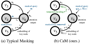
Figure 5: Comparison between typical masking used in [55, 26, 56] and our proposed correlation-adjusted masking (CaM) on graphs, where $v_{3},v_{4},v_{5}$ connected with $v_{6}$ at time $t_{5},t_{6},t_{7}$ respectively and $t$ signifies the future time of interest. We add time embedding TE($t_{3}$), TE($t_{5}$) to key nodes $v_{3},v_{5}$ and TE($t$) to query node $v_{6}$.

4.2 Correlation-adjusted Masking on Dynamic Graphs for Task-agnostic Learning

4.2.1 The Proposed Masking-based Learning Paradigm

Before delving into our paradigm, we review recent masked graph models[55, 26, 56] that replace a random part of nodes with special tokens. Let $\mathbf{m}$ denote the embedding of masked query node $v_{u}$, then the attention output is:

$$\mathbf{h}_{u}\!=\!\sum_{i\in\mathcal{N}_{u}}\!\!\left(\frac{\exp\left(e_{u,i}(\mathbf{m},\mathbf{k}_{i})\right)}{\sum_{i^{\prime}}\exp\left(e_{u,i^{\prime}}(\mathbf{m},\mathbf{k}_{i}^{\prime})\right)}\right)\mathbf{v}_{i},$$ (28)

where $\mathbf{k}_{i}$ is the embedding of the neighbor $i\in\mathcal{N}$. We note that different queries that are masked will share embedding $\mathbf{m}$, which indicates that the importance of different keys (indicated by the learned attention scores) are shared across these queries. This encourages the attention to have a global ranking of influential nodes, which makes sense in many link prediction applications such as recommender systems, as it exploits the items with high click-through rates. However, in some applications (e.g., traffic forecasting in Table I) localized ranking of influential nodes might be desired.

To address the above issue, we design a new correlation-adjusted masking method, called CaM. Specifically, let $\mathcal{M}_{u}$ denote the set of masked keys which will be removed and not used during training, and $\mathbf{q}(\mathbf{y}_{u})$ represents the label-aware embedding of masked query (e.g., $\mathbf{q}(\mathbf{y}_{u})=\mathbf{W}\mathbf{y}_{u}$). We then add sinusoidal temporal encodings to all keys and queries; without this, masked nodes will have no information about their location on dynamic graph:

$$\mathrm{TE}(t,i)=\left\{\begin{array}[]{ll}\sin(t/10000^{j/d}),\quad\quad\,\mathrm{if}~{}i~{}\mathrm{is~{}even},\\ \cos(t/10000^{j-1/d}),\quad\mathrm{if}~{}i~{}\mathrm{is~{}odd}.\end{array}\right.$$ (31)

where for key $v_{i}\in\mathcal{N}_{u}$, $t$ is time point of previous event on the pair ($v_{u},v_{i}$), whereas for query $v_{u}$ it is the future time in request. We note that it is challenging to perform positional encoding technique (e.g.,[58, 36]) on dynamic graphs due to the evolving graph structures that require to recompute Laplacian eigenmap multiple times. To that end, we compute the attention output $\mathbf{h}_{u}$ for masked query by:

$$\mathbf{h}_{u}\!=\!\!\!\sum_{i\in\mathcal{N}_{u}-\mathcal{M}_{u}}\!\!\left(\frac{\exp\Big{(}e_{u,i}(\mathbf{q}(\mathbf{y}_{u}),\mathbf{k}_{i})\Big{)}}{\sum_{i^{\prime}}\exp\Big{(}e_{u,i^{\prime}}(\mathbf{q}(\mathbf{y}_{u}),\mathbf{k}_{i}^{\prime})\Big{)}}\right)\mathbf{v}_{i},$$ (32)

where recall that $\mathcal{M}_{u}$ denotes the set of masked keys. As shown in Fig. 5, we summarize the difference between our CaM method and typical masking[55, 26, 56] on graph that randomly replaces node features with special tokens:

1. Typical masking methods replace masked key nodes with special tokens whose embedding is shared and represented by $\mathbf{m}$, whereas we remove these masked key nodes. Even though both these two methods can create diversified training examples in multi-epoch training, our method operates only on a subset of graph nodes, resulting in a large reduction in computation and memory usage.

2. We add temporal embeddings to all keys and queries, which helps the model to focus on recently formed edges (recall that in our setting, $t$ in Eq. (31) signifies time point of previous event for key nodes) and certain past timestamps.

3. We adopt label-aware embedding $\mathbf{q}(\mathbf{y}_{u})$ to represent the masked query node rather than the shared embedding $\mathbf{m}$. Equation (32) shows that the key whose embedding $\mathbf{k}_{i}$ is closer to $\mathbf{q}(\mathbf{y}_{u})$ will contribute more to the output $\mathbf{h}_{u}$. This essentially encourages the attention to focus on the keys that are highly correlated with the query label. We note that typical masking is a special case of CaM when $\mathbf{y}_{u}$ consists only of ones but no zeros (also known as positive-unlabeled learning[15]). This setting is very common in recommender systems where only “likes” (i.e., ones) are observed.

4.2.2 Task I: Masked Learning for Dynamic Link Prediction

Task Formulation. The problem of link prediction is motivated in domains such as recommender systems. As defined in Definition 4, our goal in this case is to predict which item a user will purchase at a given future timestamp, based on the observation of a past time window.

Event. This work is focused on the edge-addition events which correspond to new user-item feedbacks in the context of recommender systems. This definition of event can address the core of the recommendation problem.

Training Loss. Fig. 4(b) presents the details about model encoding and training for link prediction. Given one user’s history $\mathcal{N}_{u}$, at each time $t_{i}$ we have the embedding $\mathbf{h}_{i;L}^{\mathrm{(t_{i})}}$ for node $v_{i}$ that is used to produce an output distribution:

$$\hat{\mathbf{y}}_{u}^{(t_{i})}=\text{softmax}(\mathbf{h}_{i;L}^{\mathrm{(t_{i})}}\mathbf{W}^{O}+\mathbf{b}^{O})$$ (33)

where $\mathbf{W}^{O}\!\in\!\mathbb{R}^{d\times{N}},\mathbf{b}^{O}\!\in\!\mathbb{R}^{N}$ are the model parameters and $N,d$ are separately the number of nodes and the embedding size. To optimize the overall parameters $\Theta$, we minimize the following objective function:

$$\ell(\Theta)=\mathbf{E}_{u}\frac{1}{|\mathcal{M}_{u}|}\sum_{i,i^{\prime}\in{\mathcal{M}_{u}}}-\hat{\mathbf{y}}_{u,i}^{(t_{i})}\log(\mathbf{y}_{u,i^{\prime}}^{(t_{i})})-\gamma\mathbf{E}_{u}\,R(\Theta;u),$$

where $\mathbf{y}_{u,i^{\prime}}^{(t_{i})}=1$ means that user $u$ bought item $i^{\prime}$ at time $t_{i}$, such that $\mathbf{y}_{u,i^{\prime}}^{(t_{i})}=1$ only when $i^{\prime}=i$ and $\mathbf{y}_{u,i^{\prime}}^{(t_{i})}=0$ otherwise; $R(\Theta;u)$ represents the TPPLE term and $\mathcal{M}_{u}$ denotes the set of the masked nodes. We note that the model could trivially predict the target node in multi-layered architectures, and hence the model is trained only on the masked nodes.

Inference. In training, the model predicts each masked node $v_{i}$ with the embedding $\mathbf{q}(\mathbf{y}^{(t_{i})}_{u,i})$, where $\mathbf{y}^{(t_{i})}_{u,i}=1$ for all $v_{i}\in\mathcal{N}_{u}$. Hence, the embedding $\mathbf{q}(1)$ is shared across all masked nodes $v_{i}\in\mathcal{M}_{u}$ and does not disclose the identity of underlying node $v_{i}$. To predict the future behaviors at testing stage, we append $\mathbf{q}(1)$ to the end of the sequence $\mathcal{N}_{u}$, then exploit its output distribution to make predictions.

4.2.3 Task II: Masked Learning for Dynamic Node Classification

Task Formulation. Node classification is one of the most widely adopted tasks for evaluating graph neural networks, and as defined in Definition 5, the algorithm is designed to label every node with a categorical class at a future time point, given the observation of the history time window.

Event. Likewise, we focus on the edge-addition events. For example, on the Elliptic dataset, a new edge can be viewed as a flow of bitcoins from one transaction (node) to the next.

Training Loss. Fig. 4(c) presents the details about model encoding and training for node classification. Given $\mathcal{N}_{u}$, we compute $\mathbf{h}^{(t_{u})}_{u;L}$ for query $v_{u}$ by stacking $L$ layers to predict $\mathbf{y}_{u}^{(t_{u})}$ at time $t_{u}$ (e.g., the time of next event on query $v_{u}$):

$$\hat{\mathbf{y}}_{u}^{(t_{u})}=\operatorname{softmax}(\mathbf{h}^{(t_{u})}_{u;L}\mathbf{W}^{O})+\mathbf{b}^{O},$$ (34)

where $\mathbf{W}^{O}\!\in\!\mathbb{R}^{d\times{C}},\mathbf{b}^{O}\!\in\!\mathbb{R}^{C}$ are the model parameters and $C$ is the number of classes while $d$ is the embeddings size. To the end, we optimize the overall model parameters $\Theta$ by minimizing the following cross-entropy loss:

$$\ell(\Theta)\!=\!\mathbf{E}_{u\in\mathbb{V}}\mathrm{CrossEntropy}(\mathbf{y}_{u}^{(t_{u})},\hat{\mathbf{y}}_{u}^{(t_{u})})-\gamma\mathbf{E}_{u}\,R(\Theta;u),$$

where note that the loss is computed on all nodes $\mathbb{V}$, not limited to the masked ones. We empirically found that this stabilizes the training and increases the performance.

Inference. During training, the embedding $\mathbf{q}(\mathbf{y}^{(t_{u})}_{u})$ for masked queries is derived from the label $\mathbf{y}^{(t_{u})}_{u}$ which is not available in testing phase. Therefore, we disable the masking and use original node features $\mathbf{X}$, i.e., $\mathbf{H}_{0}=\mathbf{W}\mathbf{X}$ as model input. Warn that training the model solely on masked nodes will introduce a mismatch between the training and testing, which hurts the performance in general.

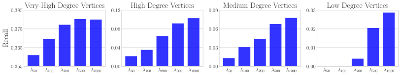
Figure 6: Recall results of very-high degree vertices (left), high degree vertices (left middle), medium degree vertices (right middle) and low degree vertices (right) for link prediction on Netflix, where $\lambda_{50}$ corresponds to GSIMC [6] by using representations with a frequency not greater than $\lambda_{50}$ to make predictions. The results show that low(high)-frequency representations reflect the user preferences on the popular(cold) items.

4.2.4 Task III: Masked Learning for Node Traffic Forecasting

Task Formulation. Traffic forecasting is the core component of intelligent transportation systems. As defined in Definition 6, the goal is to predict the future traffic speed readings on road networks given historical traffic data.

Event. In traffic networks, one road that is connected to congested roads would likely be congested. To account for this, when a road is congested, we regard it as the events of edge addition happening on its connected roads. To be more specific, we define the traffic congestion on a road when its traffic reading is significantly lower than hourly mean value at the $95\%$ confidence level.

Training Loss. Fig. 4(d) presents the details about model encoding and training for node traffic forecasting. Likewise, we predict the reading $\mathbf{y}^{(t)}_{u}$ at time $t$ (e.g., 15 min later) for road $v_{u}$ based on the time-conditioned representation $\mathbf{h}^{(t)}_{u;L}$:

$$\hat{\mathbf{y}}_{u}^{(t)}=\left\langle\mathbf{h}^{(t)}_{u;L},\mathbf{w}^{O}\right\rangle+{b}^{O},$$ (35)

where $\mathbf{w}^{O}\!\in\!\mathbb{R}^{d},{b}^{O}\!\in\!\mathbb{R}$ are the model parameters and $d$ is the embeddings size. To optimize the model parameters $\Theta$, we minimize the following least-squared loss:

$$\ell(\Theta)=\mathbf{E}_{u\in\mathbb{V}}\Big{(}\mathbf{y}_{u}^{(t)}-\hat{\mathbf{y}}_{u}^{(t)}\Big{)}^{2}-\gamma\mathbf{E}_{u}\,R(\Theta;u),$$

where the loss is computed on all nodes $\mathbb{V}$.

Inference. Analogous to the treatment for node classification, we switch off the masking and utilize original node features as the input at testing stage.

5 Interpreting: Global Analysis with Scalable and Stable Graph Spectral Analysis

This section introduces a spectral perturbation technique to interpret the model output in the graph Fourier domain. To deal with very large graphs, a scalable and orthogonalized graph Laplacian decomposition algorithm is developed.

5.1 Graph Fourier Transform

Definition 8 (Graph Signal).

Given any graph $\mathcal{G}$, the values residing on a set of nodes is referred as a graph signal. In matrix notation, graph signal can be represented by a vector $\mathbf{h}\!\in\!\mathbb{R}^{N}$ where $N$ is the number of nodes in graph $\mathcal{G}$.

Let $\mathbf{H}^{(t)}$ ($\mathbf{Y}^{(t)}$) denote the embeddings (predictions) for each node at time $t$ where each $N$-size column of $\mathbf{H}^{(t)}$ ($\mathbf{Y}^{(t)}$) can be viewed as graph signal. In what follows, we consider signal’s representations in the graph Fourier domain.

Definition 9 (Graph Fourier Transform).

Let $\{\mathbf{u}_{l}\}$ and $\{\lambda_{l}\}$ denote the eigenvectors and eigenvalues of graph Laplacian $\mathbf{L}=\mathbf{I}-\mathbf{D}^{-1/2}\mathbf{A}\mathbf{D}^{-1/2}$ where $\mathbf{D}$ is a diagonal degree matrix and $\mathbf{A}$ represents the affinity matrix, then for signal $\mathbf{f}\!\in\!\mathbb{R}^{N}$, we define the graph Fourier transform and its inverse by:

$$\widetilde{\mathbf{f}}(\lambda_{l})=\sum_{i=0}^{N-1}\mathbf{f}(i)\mathbf{u}_{l}(i)\quad\text{and}\quad\mathbf{f}(i)=\sum_{l=0}^{N-1}\hat{\mathbf{f}}(\lambda_{l})\mathbf{u}_{l}(i).$$ (36)

where in Fourier analysis on graphs[46], the eigenvalues $\{\lambda_{l}\}$ carry a notion of frequency: for $\lambda_{l}$ close to zero (i.e., low frequencies), the associated eigenvector varies litter between connected vertices.

For better understanding, Fig. 6 presents case studies in recommender systems on the Netflix prize data[3]. Specifically, we divide the item vertices into four classes: very-high degree ($>\!5000$), high degree ($>\!2000$), medium degree ($>\!100$) and low degree vertices. Then, we report the recall results of spectral graph model GSIMC[6] on four classes by only passing signals with a frequency not greater than $\lambda_{50},\dots,\lambda_{1000}$ to make top-$100$ recommendations. One can see that: 1) the low-frequency signals with eigenvalues less than $\lambda_{100}$ contribute nothing to low degree vertices; 2) the high-frequency signals with eigenvalues greater than $\lambda_{500}$ do not help increase the performance on very-high degree vertices. This finding reveals that low (high)-frequency signals reflect user preferences on popular (cold) items.

5.2 Model-Level Interpreting in Graph Fourier Domain

Most prior works on interpretable graph learning mainly often deal with the instance-level explanations in the graph vertex domain[66], e.g., in terms of the importance of node attributes indicated by the learned attention coefficients[16] and (sub)graph topologies based on the Shapley value [67].

It has been extensively discussed in recent survey [66] that the methods for model-level explanations are less studied, and existing works [65, 39] require extra training of reinforcement learning models.

By contrast, we aim at providing a global view of trained graph models in the graph Fourier domain. Compared with the explanations [65, 39] in vertex domain, it has a distinctive advantage since the frequency characterizes the smoothness of a graph signal (e.g., model predictions) with respect to the underlying graph structure. However, it is challenging to achieve this: 1) GFT itself is not capable of precisely quantifying the the predictive power of frequency content that a graph model learns from the data, and 2) it is difficult to perform GFT on large graphs due to the $\mathcal{O}(N^{3})$ cost of orthogonalized graph Laplacian decomposition.

5.2.1 Spectral Perturbation on Graphs

To enable the full explanatory power of GFT, we devise appropriate perturbations in the graph Fourier domain and measure their resulting change in prediction accuracy. Let $\mathcal{S}$ denote the frequency band (e.g., greater than $\lambda_{500}$), column $\hat{\mathbf{y}}$ denotes the predictions (e.g., predicted user behaviors on all item nodes $\mathbb{V}$), then we define the intra-perturbations:

$$\textit{perturb.}~{}\hat{\mathbf{y}}=\hat{\mathbf{y}}-\sum_{l\in\mathcal{S}}\mathbf{u}_{l}\mathbf{u}_{l}^{\top}\hat{\mathbf{y}}$$ (37)

where $\{\mathbf{u}_{l}\}$ denotes the Laplacian eigenvectors. Essentially, Eq. (37) rejects the frequency content of signal $\hat{\mathbf{y}}$ in band $\mathcal{S}$.

Proposition 1.

Given $\textit{perturb.}~{}\hat{\mathbf{y}}$ which is perturbed by Eq. (37), its Fourier transform does not have support in $\mathcal{S}$, i.e.,

$$\widetilde{\textit{perturb.}}~{}\hat{\mathbf{y}}(\lambda_{l})=0\quad\text{for}\quad\lambda_{l}\in\mathcal{S}.$$

Proof.

Following Eq. (36), for $\lambda_{l}\in\mathcal{S}$ we have

$$\widetilde{\textit{perturb.}}~{}\hat{\mathbf{y}}(\lambda_{l})=\mathbf{u}_{l}^{\top}\hat{\mathbf{y}}-\mathbf{u}_{l}^{\top}\sum_{l^{\prime}\in\mathcal{S}}\mathbf{u}_{l^{\prime}}\mathbf{u}_{l^{\prime}}^{\top}\hat{\mathbf{y}}=\mathbf{u}_{l}^{\top}\hat{\mathbf{y}}-\mathbf{u}_{l}^{\top}\hat{\mathbf{y}}=0,$$

where $\mathbf{u}_{l}^{\top}\mathbf{u}_{l^{\prime}}=1$ if $l=l^{\prime}$ and $\mathbf{u}_{l}^{\top}\mathbf{u}_{l^{\prime}}=0$ otherwise. ∎

In practice, it is of importance to precisely quantify the predictive power of different frequency contents across two models. For instance, to exaimine if dynamic graph model $\hat{\mathbf{y}}_{1}$ (e.g., BERT4REC[54]) outperforms static graph model $\hat{\mathbf{y}}_{2}$ (e.g., GSIMC[6]) due to better content at high frequencies $\mathcal{S}$ or not. To fulfill this, we propose the inter-perturbations:

$$\hat{\mathbf{y}}_{1}~{}\textit{perturb.}~{}\hat{\mathbf{y}}_{2}=\hat{\mathbf{y}}_{2}-\sum_{l\in\mathcal{S}}\mathbf{u}_{l}\mathbf{u}_{l}^{\top}\hat{\mathbf{y}}_{2}+\sum_{l\in\mathcal{S}}\mathbf{u}_{l}\mathbf{u}_{l}^{\top}\hat{\mathbf{y}}_{1},$$ (38)

where the frequency content of $\hat{\mathbf{y}}_{2}$ in band $\mathcal{S}$ is replaced by that of $\hat{\mathbf{y}}_{1}$.

Proposition 2.

Given $\hat{\mathbf{y}}_{1}~{}\textit{perturb.}~{}\hat{\mathbf{y}}_{2}$ in Eq. (38), it satisfies

$$\hat{\mathbf{y}}_{1}~{}\widetilde{\textit{perturb.}}~{}\hat{\mathbf{y}}_{2}(\lambda_{l})=\left\{\begin{array}[]{ll}\tilde{\mathbf{y}}_{2}(\lambda_{l}),\quad\quad\,\mathrm{if}~{}\lambda_{l}\notin\mathcal{S},\\ \tilde{\mathbf{y}}_{1}(\lambda_{l}),\quad\quad\,\mathrm{if}~{}\lambda_{l}\in\mathcal{S}.\end{array}\right.$$ (41)

where $\widetilde{\mathbf{y}}_{1}(\lambda_{l})$ and $\widetilde{\mathbf{y}}_{2}(\lambda_{l})$ signify the information of $\hat{\mathbf{y}}_{1}$ and $\hat{\mathbf{y}}_{2}$ at frequency $\lambda_{l}$ in the graph Fourier domain, respectively.

Proof.

As Eq. (38) only changes the content in band $\mathcal{S}$, it is trivial to conclude $\hat{\mathbf{y}}_{1}~{}\widetilde{\textit{perturb.}}~{}\hat{\mathbf{y}}_{2}(\lambda_{l})=\widetilde{\mathbf{y}}_{2}(\lambda_{l})$ for $\lambda_{l}\notin\mathcal{S}$. Then for $\lambda_{l}\in\mathcal{S}$, applying Eq. (36) leads to

$$\hat{\mathbf{y}}_{1}~{} \widetilde{\textit{perturb.}}~{}\hat{\mathbf{y}}_{2}(\lambda_{l})$$

$$=\mathbf{u}_{l}^{\top}\hat{\mathbf{y}}_{2}-\mathbf{u}_{l}^{\top}\sum_{l^{\prime}\in\mathcal{S}}\mathbf{u}_{l^{\prime}}\mathbf{u}_{l^{\prime}}^{\top}\hat{\mathbf{y}}_{2}+\mathbf{u}_{l}^{\top}\sum_{l^{\prime}\in\mathcal{S}}\mathbf{u}_{l^{\prime}}\mathbf{u}_{l^{\prime}}^{\top}\hat{\mathbf{y}}_{1}$$

$$=\mathbf{u}_{l}^{\top}\hat{\mathbf{y}}_{2}-\mathbf{u}_{l}^{\top}\hat{\mathbf{y}}_{2}+\mathbf{u}_{l}^{\top}\hat{\mathbf{y}}_{1}$$

$$=\mathbf{u}_{l}^{\top}\hat{\mathbf{y}}_{1}=\widetilde{\mathbf{y}}_{1},$$

where $\mathbf{u}_{l}^{\top}\mathbf{u}_{l^{\prime}}=1$ if $l=l^{\prime}$ and $\mathbf{u}_{l}^{\top}\mathbf{u}_{l^{\prime}}=0$ otherwise. ∎

We highlight the qualitative results in Sec. 6.3 that shows BERT4REC takes benefit of high-frequency signals ($>\lambda_{500}$) to achieve better accuracy than GSIMC on Netflix data.

TABLE III: Hit-Rate (HR) on the Koubei, Tmall and Netflix datasets for dynamic link prediction, where our model is compared against spatial graph models (i.e., GAT[59] and SAGE[23]), spectral graph models (i.e., GCN[31], ChebyNet[12], ARMA[4], MRFCF[52], GSIMC and BGSIMC[6]), sequential recommendation models (i.e., GRU4REC[25], SASREC[28], GREC[64], S2PNM[8] and BERT4REC[54]) and continuous-time graph models (i.e., DyREP[57], TGAT[61], TiSASREC[35], TGREC[17], TimelyREC[10] and CTSMA[7]). Bolded numbers denote the best, and the standard errors of the ranking metrics are less than 0.01 for all the results. ^∗Conference version of this work based on which we obtain the relative gain.

	Koubei, Density=$\mathbf{0.08\%}$				Tmall, Density=$\mathbf{0.10\%}$				Netflix, Density=$\mathbf{1.41\%}$
Model	HR@10	HR@50	HR@100		HR@10	HR@50	HR@100		HR@10	HR@50	HR@100
GAT [59]	0.19715	0.26440	0.30125		0.20033	0.32710	0.39037		0.08712	0.19387	0.27228
SAGE [23]	0.20600	0.27225	0.30540		0.19393	0.32733	0.39367		0.08580	0.19187	0.26972
GCN [31]	0.20090	0.26230	0.30345		0.19213	0.32493	0.38927		0.08062	0.18080	0.26720
ChebyNet [12]	0.20515	0.28100	0.32385		0.18163	0.32017	0.39417		0.08735	0.19335	0.27470
ARMA [4]	0.20745	0.27750	0.31595		0.17833	0.31567	0.39140		0.08610	0.19128	0.27812
MRFCF [52]	0.17710	0.19300	0.19870		0.19123	0.28943	0.29260		0.08738	0.19488	0.29048
GSIMC [6]	0.23460	0.31995	0.35065		0.13677	0.31027	0.40760		0.09725	0.22733	0.32225
BGSIMC [6]	0.24390	0.32545	0.35345		0.16733	0.34313	0.43690		0.09988	0.23390	0.33063
GRU4REC [25]	0.26115	0.33495	0.37375		0.24747	0.37897	0.44980		0.23442	0.40445	0.49175
SASREC [28]	0.24875	0.32805	0.36815		0.25597	0.39040	0.45803		0.22627	0.39222	0.48085
GREC [64]	0.23831	0.31533	0.35431		0.22470	0.35057	0.41507		0.24338	0.41690	0.50483
S2PNM [8]	0.26330	0.33770	0.37730		0.25470	0.38820	0.45707		0.24762	0.42160	0.50858
BERT4REC [54]	0.25663	0.33534	0.37483		0.26810	0.40640	0.47520		0.25337	0.43027	0.52115
DyREP [57]	0.26360	0.33490	0.37150		0.25937	0.38593	0.44903		0.22883	0.40997	0.50093
TGAT [61]	0.25095	0.32530	0.36195		0.26070	0.39533	0.46503		0.22755	0.39623	0.48232
TiSASREC [35]	0.25295	0.33115	0.37110		0.26303	0.40463	0.47390		0.24355	0.41935	0.50767
TGREC [17]	0.25175	0.31870	0.35655		0.24577	0.37960	0.44827		0.22733	0.38415	0.47170
TimelyREC [10]	0.25565	0.32835	0.37085		0.24280	0.36853	0.43240		0.23018	0.39772	0.48608
CTSMA [7] (conference ver.)	0.27460	0.35250	0.39240		0.26760	0.40477	0.47310		0.25405	0.43723	0.52613
EasyDGL (ours)	0.29285	0.39280	0.44005		0.27657	0.42063	0.49317		0.29098	0.47395	0.56178
Rel. Gain (over [7])	6.6%	11.4%	12.1%		3.2%	3.5%	3.8%		14.5%	8.4%	6.7%

5.2.2 Scalable Graph Laplacian Decomposition for Graph Fourier Transforms with Orthogonality

To address the scalability issue, we propose a scalable and orthogonalized graph Laplacian decomposition algorithm, which differs to [32, 22] as the approximate eigenvectors are not orthogonal in these works. Note that orthogonality makes signal’s spectral representation computing fast and avoid the frequency components of signal’s spectrum interacting with each other in terms of frequency which thus could provide a more clean interpretability.

Specifically, we uniformly sample an $s$-column submatrix $\mathbf{C}$ from graph Laplacian matrix $\mathbf{L}$ and then define the normalized matrix $\mathbf{W}$ by following [19]:

$$\mathbf{C}=\left[\begin{array}[]{l}\mathbf{A}\\ \mathbf{B}^{\top}\end{array}\right]\quad\mathrm{and}\quad\mathbf{W}=\mathbf{A}^{-1/2}\mathbf{C}^{\top}\mathbf{CA}^{-1/2}.$$ (44)

We adopt the randomized algorithm [22] to approximate the eigenvectors of matrix $\mathbf{W}$ as an initial solution $(\mathbf{\Sigma}_{W},\mathbf{U}_{W})$, then by running the Nystr$\mathrm{\ddot{o}}$m method [19] to extrapolate this solution to the full matrix $\mathbf{L}$.

Algorithm 1 Scalable and Orthogonalized Graph Laplacian Decomposition for Graph Fourier Transforms

0:  matrix $\mathbf{C}\in\mathcal{R}^{N\times{s}}$ derived from $s$ columns sampled from matrix $\mathbf{L}\!\in\!\mathcal{R}^{N\times{N}}$ without replacement, matrix $\mathbf{A}\!\in\!\mathcal{R}^{s\times{s}}$ composed of the intersection of these $s$ columns, matrix $\mathbf{W}\!\in\!\mathcal{R}^{s\times{s}}$, rank $r$, the oversampling parameter $p$ and the number of power iterations $q$.

0:  eigenvalues $\widetilde{\mathbf{\Sigma}}$ and eigenvectors $\mathbf{\widetilde{U}}$.

1:  Generate a random Gaussian matrix $\mathbf{\Omega}\in\mathbb{R}^{s\times{(r+p)}}$, then compute the sample matrix $\mathbf{A}^{q}\mathbf{\Omega}$.

2:  Perform QR-Decomposition on $\mathbf{A}^{q}\mathbf{\Omega}$ to obtain an orthonormal matrix $\mathbf{Q}$ that satisfies the equation $\mathbf{A}^{q}\mathbf{\Omega}=\mathbf{QQ}^{\top}\mathbf{A}^{q}\mathbf{\Omega}$, then solve $\mathbf{ZQ}^{\top}\mathbf{\Omega}=\mathbf{Q}^{\top}\mathbf{W\Omega}$.

3:  Compute the eigenvalue decomposition on the $(r+p)$-by-$(r+p)$ matrix $\mathbf{Z}$, i.e., $\mathbf{Z}=\mathbf{U_{Z}\Sigma_{Z}{U}_{Z}}^{\top}$, to obtain $\mathbf{U}_{W}=\mathbf{QU}_{Z}[:,:r]$ and $\mathbf{\Sigma}_{W}=\mathbf{\Sigma}_{Z}[:r,:r]$.

4:  Return $\widetilde{\mathbf{\Sigma}}\leftarrow\mathbf{\Sigma}_{W}$, $\mathbf{\widetilde{U}}\leftarrow\mathbf{CA}^{-1/2}\mathbf{U}_{W}\mathbf{\Sigma}_{W}^{-1/2}$.

The pseudo-code is provided in Algorithm 1. To summarize, the computational complexity is $\mathcal{O}(Nsr+r^{3})$ where $N,s,r$ is the number of nodes, sampled columns and eigenvectors, respectively. Recall that typically $N\!\gg\!{s}\!\geq\!{r}$, and hence our Algorithm 1 has a lower complexity than typical Nystr$\mathrm{\ddot{o}}$m method, i.e., $\mathcal{O}(Nsr+s^{3})$ in [32].

5.2.3 Error Bound of Algorithm 1

We further analyze the error bound of Algorithm 1 with respect to the spectral norm. Theorem 1 suggests that our Algorithm 1 is as accurate as typical Nystr$\mathrm{\ddot{o}}$m method (i.e., $\parallel\mathbf{L}-\widetilde{\mathbf{L}}\parallel_{2}+\frac{N}{\sqrt{s}}\mathbf{L}^{\ast}_{i,i}$ in Corollary 2[32]) when the number of power iterations $q$ is large enough, while our algorithm fulfills the orthogonality constraint. The proof details are provided in https://thinklab.sjtu.edu.cn/project/EasyDGL/suppl.pdf (see also in the supplemental material).

Theorem 1 (Error Bound).

For $\widetilde{\mathbf{L}}=\mathbf{\widetilde{U}\widetilde{\Sigma}\widetilde{U}}^{\top}$ in Algorithm 1, and $\zeta=1+\sqrt{\frac{r}{p-1}}+\frac{e\sqrt{r+p}}{p}\sqrt{s-r}$,

$$\mathbf{E}\parallel\mathbf{L}-\widetilde{\mathbf{L}}\parallel_{2}\leq\zeta^{1/q}\parallel\mathbf{L}-\widetilde{\mathbf{L}}_{r}\parallel_{2}+\left(1+\zeta^{1/q}\right)\frac{N}{\sqrt{s}}\mathbf{L}^{\ast}_{i,i},$$

where $\mathbf{L}^{\ast}_{i,i}=\max_{i}\mathbf{L}_{i,i}$ and $\mathbf{L}_{r}$ is the best rank-$r$ approximation.

6 Experiments and Discussion

The experiments evaluate the overall performance of our pipeline EasyDGL as well as the effects of its components including TPPLE and CaM. We further perform qualitative analysis to provide a global view of both static graph models and dynamic graph models. Experiments are conducted on Linux workstations with Nvidia RTX8000 (48GB) GPU and Intel Xeon W-3175X CPU@ 3.10GHz with 128GB RAM. The source code is implemented by the Deep Graph Library (DGL, https://www.dgl.ai/) hence our approach name easyDGL also would like to respect this library.

6.1 Evaluation of Overall Performance

6.1.1 Dynamic Link Prediction

Dataset. We adopt three large-scale real-world datasets: (1) Koubei ($223,044$ nodes and $1,828,250$ edges); (2) Tmall ($342,373$ nodes and $7,632,826$ edges); (3) Netflix ($497,959$ nodes and $100,444,166$ edges). For each dataset, a dynamic edge $(v_{u},v_{i},t_{k})$ indicates if user (i.e., node) $v_{u}$ purchased item (i.e., node) $v_{i}$ at time $t_{k}$. Note that these datasets are larger than Wikidata ($11,134$ nodes and $150,079$ edges), Reddit ($55,863$ nodes and $858,490$ edges).

TABLE IV: NDCG (N) on Koubei, Tmall and Netflix for dynamic link prediction. The standard errors of the ranking metrics are all less than 0.005.

	Koubei, Density=$\mathbf{0.08\%}$				Tmall, Density=$\mathbf{0.10\%}$				Netflix, Density=$\mathbf{1.41\%}$
Model	N@10	N@50	N@100		N@10	N@50	N@100		N@10	N@50	N@100
GAT [59]	0.15447	0.16938	0.17534		0.10564	0.13378	0.14393		0.04958	0.07250	0.08518
SAGE [23]	0.15787	0.17156	0.17701		0.10393	0.13352	0.14417		0.04904	0.07155	0.08419
GCN [31]	0.15537	0.16848	0.17548		0.10287	0.13208	0.14260		0.04883	0.06965	0.08456
ChebyNet [12]	0.15784	0.17406	0.18055		0.09916	0.12955	0.14175		0.04996	0.07268	0.08582
ARMA [4]	0.15830	0.17320	0.17954		0.09731	0.12628	0.13829		0.04940	0.07192	0.08526
MRFCF [52]	0.10037	0.10410	0.10502		0.08867	0.11223	0.11275		0.05235	0.08047	0.09584
GSIMC [6]	0.17057	0.18970	0.19468		0.07357	0.11115	0.12661		0.05504	0.08181	0.09759
BGSIMC [6]	0.17909	0.19680	0.20134		0.09222	0.13082	0.14551		0.05593	0.08400	0.09982
GRU4REC [25]	0.20769	0.22390	0.23017		0.16758	0.19641	0.20770		0.14908	0.18648	0.20064
SASREC [28]	0.19293	0.21173	0.21612		0.17234	0.20207	0.21292		0.14570	0.18209	0.19644
GREC [64]	0.19115	0.20769	0.21445		0.14969	0.17750	0.18775		0.15674	0.19455	0.20894
S2PNM [8]	0.20538	0.22171	0.22812		0.17250	0.20210	0.21335		0.15902	0.19750	0.21141
BERT4REC [54]	0.19944	0.21685	0.22325		0.18042	0.21096	0.22193		0.16274	0.20166	0.21638
DyREP [57]	0.21086	0.22684	0.23240		0.17290	0.20071	0.21092		0.14593	0.18567	0.20043
TGAT [61]	0.19803	0.21347	0.21933		0.17497	0.20419	0.21533		0.14541	0.18219	0.19611
TiSASREC [35]	0.19731	0.21518	0.22153		0.17502	0.20609	0.21754		0.15455	0.19272	0.20687
TGREC [17]	0.19829	0.21226	0.21807		0.16378	0.19334	0.20457		0.14877	0.18285	0.19711
TimelyREC [10]	0.20530	0.22036	0.22725		0.16656	0.19434	0.20472		0.14615	0.18301	0.19734
CTSMA [7] (conference ver.)	0.21059	0.22767	0.23396		0.18020	0.21039	0.22164		0.16137	0.20172	0.21613
EasyDGL (ours)	0.22627	0.24838	0.25629		0.21511	0.23313	0.23973		0.18667	0.22688	0.24116
Rel. Gain (over [7])	7.4%	9.1%	9.5%		19.2%	10.8%	8.0%		14.7%	12.4%	11.4%

Protocol. We follow the inductive experimental protocol [38] together with the dynamic protocol [57] to evaluate the learned node representations, where the goal is to predict which is the most likely node $v$ that a given node $u$ would connect to at a specified future time $t$. Note that test node $u$ is not seen in training and the time $t$ can be arbitrary in different queries. To do so, we split user nodes into training, validation and test set with ratio $8\!:\!1\!:\!1$, where all the data from the training users are used to train the model. At test stage, we sort all links of validation/test users in chronological order, and hold out the last one for testing.

The results are reported in terms of the hit rate (HR) and the normalized discounted cumulative gain (NDCG) on the test set for the model which achieves the best results on the validation set. The implementation of HR and NDCG follows [38], and the reported results are averaged over five different random data splits.

Baseline. We compare state-of-the-art baselines: (1) static graph approaches. We follow the design in IDCF[60] to generate a user’s representation by aggregating the information in her/his purchased items, then we report the performance by using different backbone GNNs, i.e., GraphSAGE[23], GAT[59], GCN[31], ChebyNet[12] and ARMA[4]. Also, we compare with shallow spectral graph models including MRFCF[4], GSIMC and BGSIMC[6]; (2) sequential recommendation approaches. GRU4REC[25] utilizes recurrent neural networks to model the sequential information, SASREC [28] and GREC[64] adopt attention networks and causal convolutional neural networks to learn the long-term patterns. S2PNM[8] proposes a hybrid memory networks to establish a balance between the short-term and long-term patterns. BERT4REC[54] extends the Cloze task to SASREC for improvements; (3) continuous-time approaches. TGAT[61], TiSASREC[35] and TGREC[17] encode the temporal information independently into embeddings. DyREP[57], TimelyREC[10] and CTSMA[7] model the entangled spatiotemporal information on the dynamic graph.

We select the Adam [30] as the optimizer and decay the learning rate every 10 epochs with a rate of 0.9. We search the embedding size in $\{64,128,\dots,512\}$, the learning rate $\{1e\!-\!5,\dots,1e\!-\!1\}$, the dropout rate $\{0.1,\dots,0.7\}$ and the $\ell_{2}$ regularizer $\{1e\!-\!5,\dots,1e\!-\!1\}$. More detailed settings for our proposed model and the baselines could be found in the supplementary material or in our open-source link.

Results. Table III and Table IV show the HR and NDCG of our EasyDGL and the baselines on the Koubei, Tmall and Netflix datasets. It is shown that sequential models achieve better results than static graph models, and continuous-time graph models (i.e., DyREP, TimelyREC, CSTMA, TiSASREC, TGREC, TiSASREC, TGAT and EasyDGL) are among the best on all three datasets. In particular, EasyDGL achieves $6.7-14.5\%$ relative hit rate gains and $11.4-14.7\%$ relative NDCG gains over the best baseline on challenging Netflix.

In addition, we emphasize EasyDGL’s consistent performance boosting over our preliminary conference version CTSMA [7]. The key difference is that CTSMA is a unidirectional autoregressive model. By contrast, EasyDGL is a bidirectional masked autoencoding model that incorporates the contexts from both left and right side. Perhaps more importantly, EasyDGL enjoys the benefit of improved robustness and generalizability, due to masking strategy that introduces the randomness to the model and also generates diversified samples for training.

TABLE V: Evaluation on the Elliptic dataset (bitcoin transactions) for dynamic node classification over time, where EasyDGL performs best for all columns at different time steps among both static graph models (top half) as well as dynamic graph models (bottom half). Note that DySAT [51], EvolveGCN [47], JODIE [33] and TGN [50] require multiple (i.e. 5) historical graph snapshots (see the ‘input’ column), whereas EasyDGL only accesses the update-to-date snapshot for prediction. EasyDGL outperforms the best baseline TGN in accuracy with 4X speedup for training. All the methods perform poorly starting at time step 43, because this time is when the bitcoin dark market shutdown occurred which changes the external environment of the graph yet such information cannot be readily encoded by the evaluated models neither in training nor testing. In this extreme case, EasyDGL performs relatively better than baselines especially regarding the Micro-F1 score which is for the minority (illicit) class.

Timestamp=[40, 42]

Timestamp=[43, 46]

Timestamp=[47, 49]

Model

Input

Macro-F1

Micro-F1

Accuracy

Macro-F1

Micro-F1

Accuracy

Macro-F1

Micro-F1

Accuracy

APPNP [52]

1

0.666$\pm$0.009

0.542$\pm$0.020

0.776$\pm$0.010

0.476$\pm$0.028

0.014$\pm$0.020

0.782$\pm$0.008

0.462$\pm$0.029

0.000$\pm$0.000

0.792$\pm$0.007

GAT [59]

1

0.660$\pm$0.021

0.517$\pm$0.085

0.754$\pm$0.016

0.465$\pm$0.010

0.018$\pm$0.018

0.731$\pm$0.017

0.452$\pm$0.024

0.013$\pm$0.028

0.735$\pm$0.043

SAGE [23]

1

0.691$\pm$0.016

0.514$\pm$0.067

0.820$\pm$0.015

0.507$\pm$0.009

0.011$\pm$0.024

0.824$\pm$0.013

0.493$\pm$0.035

0.024$\pm$0.047

0.831$\pm$0.030

ARMA [4]

1

0.707$\pm$0.031

0.556$\pm$0.050

0.825$\pm$0.007

0.512$\pm$0.027

0.041$\pm$0.024

0.826$\pm$0.009

0.498$\pm$0.021

0.016$\pm$0.036

0.834$\pm$0.012

ChebyNet [12]

1

0.682$\pm$0.014

0.517$\pm$0.031

0.800$\pm$0.024

0.499$\pm$0.030

0.000$\pm$0.000

0.790$\pm$0.040

0.472$\pm$0.037

0.000$\pm$0.000

0.795$\pm$0.050

GCN [31]

1

0.540$\pm$0.047

0.231$\pm$0.097

0.780$\pm$0.012

0.459$\pm$0.014

0.021$\pm$0.025

0.799$\pm$0.005

0.520$\pm$0.015

0.018$\pm$0.036

0.884$\pm$0.005

TGAT [61]

1

0.693$\pm$0.027

0.529$\pm$0.035

0.803$\pm$0.009

0.501$\pm$0.010

0.046$\pm$0.036

0.805$\pm$0.006

0.495$\pm$0.025

0.047$\pm$0.028

0.813$\pm$0.009

DySAT [51]

5

0.611$\pm$0.020

0.477$\pm$0.061

0.739$\pm$0.009

0.469$\pm$0.011

0.021$\pm$0.018

0.744$\pm$0.016

0.470$\pm$0.020

0.000$\pm$0.000

0.774$\pm$0.034

EvolveGCN [47]

5

0.591$\pm$0.012

0.382$\pm$0.019

0.735$\pm$0.002

0.458$\pm$0.005

0.000$\pm$0.000

0.734$\pm$0.008

0.443$\pm$0.035

0.037$\pm$0.022

0.727$\pm$0.024

JODIE [33]

5

0.696$\pm$0.021

0.486$\pm$0.064

0.814$\pm$0.017

0.525$\pm$0.011

0.025$\pm$0.030

0.836$\pm$0.009

0.544$\pm$0.008

0.000$\pm$0.000

0.873$\pm$0.011

TGN [50]

5

0.719$\pm$0.016

0.542$\pm$0.023

0.834$\pm$0.009

0.529$\pm$0.010

0.024$\pm$0.028

0.827$\pm$0.021

0.572$\pm$0.013

0.071$\pm$0.011

0.885$\pm$0.042

EasyDGL

1

0.730$\pm$0.002

0.566$\pm$0.012

0.845$\pm$0.003

0.540$\pm$0.007

0.069$\pm$0.023

0.843$\pm$0.003

0.575$\pm$0.003

0.110$\pm$0.009

0.885$\pm$0.006

TABLE VI: Evaluation on the META-LA dataset for 15 minutes (horizon 3), 30 minutes (horizon 6) and 45 minutes (horizon 9) ahead traffic forecasting, where the baselines include static graph models (top half) and dynamic graph models (bottom half). Note that DCRNN[37] , DySAT[51], GaAN[68], STGCN[63] and DSTAGNN[34] use 60 minutes as the historical time window, namely the most recent 12 graph snapshots (see the ‘input’ column) are used to forecast traffic conditions in the next 15, 30 and 45 minutes, whereas EasyDGL makes predictions only based on the current single graph snapshot. Specifically, EasyDGL performs competitively with state-of-the-art DSTAGNN with 6X speedup for training.

Horizon=3 (15 minutes)

Horizon=6 (30 minutes)

Horizon=9 (45 minutes)

Model

Input

MAE

RMSE

MAPE

MAE

RMSE

MAPE

MAE

RMSE

MAPE

APPNP [52]

1

3.987$\pm$0.010

6.708$\pm$0.015

0.117$\pm$0.000

4.496$\pm$0.011

7.769$\pm$0.017

0.137$\pm$0.000

4.902$\pm$0.008

8.579$\pm$0.021

0.156$\pm$0.001

GAT [59]

1

4.992$\pm$0.237

8.587$\pm$0.470

0.155$\pm$0.010

5.228$\pm$0.184

9.049$\pm$0.348

0.164$\pm$0.008

5.456$\pm$0.163

9.473$\pm$0.278

0.174$\pm$0.006

SAGE [23]

1

3.318$\pm$0.004

6.097$\pm$0.007

0.088$\pm$0.000

3.866$\pm$0.007

7.291$\pm$0.009

0.110$\pm$0.001

4.259$\pm$0.007

8.134$\pm$0.030

0.127$\pm$0.001

ARMA [4]

1

3.298$\pm$0.008

6.058$\pm$0.017

0.087$\pm$0.001

3.824$\pm$0.006

7.221$\pm$0.011

0.108$\pm$0.000

4.191$\pm$0.007

8.017$\pm$0.018

0.124$\pm$0.000

ChebyNet [12]

1

3.457$\pm$0.016

6.352$\pm$0.022

0.091$\pm$0.002

4.025$\pm$0.002

7.571$\pm$0.028

0.112$\pm$0.000

4.466$\pm$0.023

8.390$\pm$0.045

0.129$\pm$0.000

GCN [31]

1

5.748$\pm$0.013

9.780$\pm$0.036

0.188$\pm$0.001

5.813$\pm$0.011

9.988$\pm$0.031

0.192$\pm$0.000

5.901$\pm$0.009

10.21$\pm$0.026

0.198$\pm$0.001

DCRNN [37]

12

3.002$\pm$0.018

5.699$\pm$0.019

0.079$\pm$0.000

3.429$\pm$0.027

6.782$\pm$0.018

0.095$\pm$0.001

3.735$\pm$0.045

7.493$\pm$0.039

0.107$\pm$0.001

DySAT [51]

12

3.115$\pm$0.012

6.101$\pm$0.039

0.085$\pm$0.000

3.710$\pm$0.015

7.391$\pm$0.041

0.108$\pm$0.001

4.184$\pm$0.018

8.317$\pm$0.031

0.128$\pm$0.001

GaAN [68]

12

3.029$\pm$0.013

5.799$\pm$0.043

0.083$\pm$0.001

3.580$\pm$0.017

7.068$\pm$0.063

0.104$\pm$0.002

3.994$\pm$0.022

7.960$\pm$0.084

0.122$\pm$0.002

STGCN [63]

12

3.195$\pm$0.027

6.240$\pm$0.050

0.089$\pm$0.001

3.392$\pm$0.025

6.806$\pm$0.049

0.097$\pm$0.001

3.575$\pm$0.027

7.251$\pm$0.036

0.104$\pm$0.001

DSTAGNN [34]

12

2.960$\pm$0.035

5.611$\pm$0.052

0.079$\pm$0.001

3.321$\pm$0.030

6.683$\pm$0.056

0.093$\pm$0.001

3.595$\pm$0.029

7.249$\pm$0.058

0.102$\pm$0.000

EasyDGL

1

2.879$\pm$0.019

5.594$\pm$0.040

0.076$\pm$0.001

3.268$\pm$0.005

6.590$\pm$0.021

0.090$\pm$0.001

3.527$\pm$0.026

7.220$\pm$0.044

0.100$\pm$0.001

6.1.2 Dynamic Node Classification

Dataset. There are few datasets available for node classification in the dynamic setting. To the best of our knowledge, the Elliptic dataset is the largest one which has $203,769$ nodes and $234,355$ edges derived from the bitcoin transaction records whose timestamp is actually discrete value from 0 to 49 which are evenly spaced in two weeks. We argue that the Reddit and Wikipedia used in [61, 27] is more suitable for edge classification, because the label for a user (node) on Reddit indicates if the user is banned from posting under a subreddit (node), and likewise the label on Wikipedia is about whether the user (node) is banned from editing a Wikipedia page (node). In contrast, a node in Elliptic is a transaction and edges can be viewed as a flow of bitcoins between one transaction and the other. The label of each node indicates if the transaction is “licit”, “illicit” or “unknown”.

Protocol. The evaluation protocol follows [47], where we use the information up to (discrete) time step $t$ and predict the label of a node which appears at the next (discrete) step $t\!+\!1$. Specifically, we split the data into training, validation and test set along the time dimension, where we use the first $38$ time steps to train the model, the next two time steps as the validation set and the rest used for testing. We note that the dark market shutdown occurred at step $43$, and thus we further group the test data in time steps $[40,49]$ into subsets $[40,42]$, $[43,46]$ and $[47,49]$ to better study how the model behaves under external substantial changes.

We report the results in terms of Macro-F1, Micro-F1 and accuracy on the test set for the model that achieves the best on the validation data set. We note that nearly $80\%$ of nodes are labeled as “unknown”, such that a model which labels every node as unknown can achieve the accuracy up to $0.8$. Because the illicit nodes are of more interest, we report the Micro-F1 for the minority (illicit) class. The results are the mean from five random trials.

Baseline. We compare with state-of-the-art methods for dynamic node classification: (1) static graph approaches, i.e., APPNP [52], GAT [59], SAGE [23], ARMA [4], GCN [31] and ChebyNet [12]; (2) discrete-time approaches. DySAT[51] uses attention networks to model both temporal and structural information. Differently, EvolveGCN[47] models the evolution of parameters in GCN over time; (3) continuous-time approaches. JODIE[33] and TGAT[61] adopt linear and sinusoidal functions of the elapsed time to encode the temporal information, respectively. TGN[50] combined the merits of temporal modules in JODIE, TGAT and DyREP to achieve the performance improvement. We omit the results of CTDNE[45] and DyREP[57], since it is known (see [50, 27]) that their accuracies are lower than TGN.

The embedding size for all methods is set to $32$ for fair comparisons, and the time window size for DySAT, JODIE, TGN and EvolveGCN is $5$. The hyperparameter is searched by grid, analogous to the dynamic link prediction task.

Results. Table V compares EasyDGL with the baselines by Macro-F1, Micro-F1 and Accuracy on the Elliptic dataset. We see that ARMA performs the best among static graph models and further achieves comparable results to dynamic models: DySAT, JODIE and EvolveGCN. This is due to that ARMA provides a larger variety of frequency responses so that the network can better model sharp changes. Besides, TGN beats all other baselines, while EasyDGL obtains better results than TGN with 4X speedup for training.

In particular, all models perform poorly after time step $43$, when there was an external sudden change — the shutdown of dark market, which results in the universal performance degradation. EasyDGL achieves $68\%$ and $55\%$ relative Micro-F1 gains over the best baseline during time step $[43,46]$ and $[47,49]$, respectively. This proves the merit of EasyDGL in effective adaptation under sharp changes.

TABLE VII: Hit-Rate (HR) and NDCG (N) on the Netflix dataset for dynamic link prediction. (top) intra-perturbation is applied to remove the spectral contents of BERT4REC[54] with frequencies greater than $\lambda_{500}$. The performance degradation of the resulting perturb. BERT4REC model suggests the necessity of high-frequency information; (middle) inter-perturbation is applied to replace the high-frequency ($>\lambda_{500}$) contents of GSIMC[6] by that of BERT4REC. One can see that the BERT4REC perturb. GSIMC model performs comparable to BERT4REC. This implies that dynamic graph model BERT4REC outperforms static graph model SGMC due to the ability to learn high-frequency information; (bottom) inter-perturbation is applied to replace both low-frequency ($\leq\lambda_{50}$) and high-frequency ($\lambda_{900}-\lambda_{1000}$) contents of TGAT with that of EasyDGL. The performance improvement demonstrates the efficacy of the recommendation strategies and our superiority of modelling complex temporal dynamics over TGAT.

Netflix	HR@10	HR@50	HR@100	N@10	N@50	N@100
BERT4REC	0.25337	0.43027	0.52115	0.16274	0.20166	0.21638
perturb. BERT4REC	0.14454	0.21172	0.24198	0.09477	0.10994	0.11484
GSIMC	0.09725	0.22733	0.32225	0.05504	0.08181	0.09759
BERT4REC perturb. GSIMC	0.25287	0.42514	0.50937	0.16243	0.20033	0.21398
TGAT	0.22755	0.39623	0.48232	0.14541	0.18219	0.19611
EasyDGL perturb. TGAT	0.24832	0.42487	0.50587	0.15649	0.19550	0.20865

6.1.3 Node Traffic Forecasting

Dataset. We conduct experiments on real-world METR-LA dataset [37] from the Los Angels Metropolitan Transportation Authority, which has averaged traffic speed measured by 207 sensors every $5$ minutes on the highways. It is shown in [63, 37] that traffic flow forecasting on METR-LA ($207$ sensors, $34,272$ samples, Los Angels) is more challenging than that on PEMS-BAY ($325$ sensors, $52,116$ samples, Bay Area) dataset due to complicated traffic conditions.

Protocol. We follow the protocol used in[37] to study the performance for traffic forecasting task, where we aggregate traffic speed readings at $5$-minute level and apply z-score normalization. We utilize first $70\%$ of data for model training, $10\%$ for validation while the remaining $20\%$ data for testing. Each of compared models is allowed to leverage the traffic conditions up to now for $15/30/45$-minutes ahead forecasting. We also adopt the mean absolute error (MAE), rooted mean squared error (RMSE) as well as mean absolute percentage error (MAPE) to evaluate the model accuracies. Detailed formulations of these metrics can be found in [37].

Baseline. Existing traffic forecasting methods are mainly focused on discrete-time graphs, as the traffic data is often collected in a constant rate (e.g., every 5 minutes). These approaches maintain a sliding window of most recent 60-minutes data (i.e., $12$ snapshots) to make $15/30/45$-minutes ahead forecasting. DCRNN[37] leverages GCN to encode spatial information, while GaAN[68] uses GAT to focus on most relevant neighbors in spatial domain. These methods both exploit RNNs to capture the evolution of each node. To increase the scalability, DySAT[51] utilize attention networks to incorporate both structural and temporal dynamics while STGCN[63] resorts to simple CNNs. DSTAGNN[34] integrate the attention and gated CNN for improvements. For comparison completeness, we also report the results of static graph approaches, including APPNP[52], ChebyNet[12], GAT[59], SAGE[23], ARMA[4] and GCN[31].

Following [37, 63], the embedding size is set to $32$ and the sliding window size for discrete-time approaches, i.e., DCRNN, GaAN, DySAT, STGCN and DSTAGNN, is $12$. The hyperparameter is tuned by grid search analogous to previous tasks. Note that EasyDGL and static graph models leverage only the most recent snapshot to make multi-step traffic forecasting, or namely the window size is one. Thus, the comparison is in favor of discrete-time approaches.

Results. Table VI presents the results on the METR-LA dataset for $15/30/45$ minutes ahead forecasting. Dynamic approaches outperform static ones by a notable margin, and EasyDGL achieves the best results among baselines. We note that the protocol is in favor of discrete-time approaches: they accept $12$ graph snapshots as input, while EasyDGL accesses to only $1$ snapshot. Also, EasyDGL takes 1.1 hour training time, 6X faster than recently published DSTAGNN.

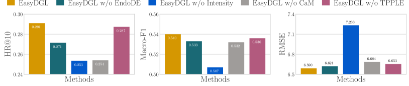
Figure 7: Ablation study on Netflix for dynamic link prediction (left), on Elliptic for dynamic node classification (middle) during step $[43,46]$, on META-LA for 30 minutes ahead traffic forecasting (right). The higher HR@10 and Macro-F1 mean are better, while lower RMSE is better.

Figure 8: Spectral interpreting of GSIMC[6], BERT4REC[54] and EasyDGL for dynamic link prediction on Netflix. The energy of GSIMC is focused on low frequencies since high-frequency signals are penalized during minimization, whereas BERT4REC and EasyDGL put more energies to high frequencies which helps increase the recall rates of low degree item nodes. This explains the performance gap between static and dynamic models.

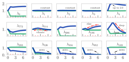
Figure 9: The energy scale factor of 15 frequencies in 15 plots by spectral interpreting of TGAT[61] (green) and EasyDGL (blue) for the dynamic link prediction models trained on Netflix, which studies how TGAT and EasyDGL behave in the graph Fourier domain over time (x-axis, in 7 days). It shows that EasyDGL amplifies low-frequency signals (e.g., $\lambda_{0},\lambda_{4}$) as time elapsed, signal at frequency $\lambda_{806}$ increases until the time interval reaches $2$ days long then drops dramatically, and high-frequency signals (e.g., $\lambda_{934},\lambda_{952}$) are attenuated as time goes on.

6.2 Ablation Study

We evaluate the effectiveness of our proposed components: EasyDGL w/o EndoDE drops endogenous dynamics encoding, making the intensity independent of localized changes. EasyDGL w/o Intensity switches off intensity-based modulation, thereby reducing our attention to regular attention. EasyDGL w/o CaM disables our masking mechanism, while EasyDGL w/o TPPLE removes the TPP posterior maximization term by setting $\gamma=0$ in Eq. (24).

Fig. 7 reports HR@10 on Netflix for dynamic link prediction, RMSE on Elliptic for dynamic node classification, and Macro-F1 on META-LA for traffic forecasting. We omit the results in other metrics (NDCG, MAE MAPE) and on other data as their trends are similar. We see that EasyDGL w/o EndoDE performs worse than EasyDGL for all three tasks which suggests the necessity of modelling entangled spatiotemporal information; EasyDGL w/o Intensity exhibits a significant drop in the performance, validating the efficacy of our TPP-based modulation design; EasyDGL w/o CaM shows worse performance, which provides an evidence to the necessity of designing mask-based learning for dynamic graph models; the performance of EasyDGL w/o TPPLE also degrades that suggests the effectiveness of our TPPLE regularization.

6.3 Qualitative Study

We conduct experiments on Netflix for qualitative study.

R1: dynamic graph approach has a distinct advantage on the ability to manipulate high-frequency signals. In Fig. 9, we analyze static GSIMC model, dynamic BERT4REC and EasyDGL models in the graph Fourier domain, where we apply $\ell_{2}$ normalization to each user’s spectral signals in test set and visualize the averaged values. It shows that GSIMC only passes low frequencies (a.k.a., low-pass filtering), while dynamic models are able to learn high-frequency signals.

In Table VII, we apply the intra-perturbation to BERT4REC in order to remove spectral content at frequencies greater than $\lambda_{500}$. We see that perturb. BERT4REC exhibits a significant drop in performance, which demonstrates the necessity of high-frequency information. Meanwhile, we use BERT4REC to perturb the predictions of GSIMC so as to measure the importance of high frequencies for GSIMC. The fact that BERT4REC perturb. GSIMC performs much better than GSIMC and comparable to BERT4REC, indicating that BERT4REC beats GSIMC due to the ability of learning high-frequency information on dynamic graph.

R2: EasyDGL tends to amplify low-frequency signal and attenuate high-frequency signal as time elapses. We retreat spectral signal for each user as a function of elapsed time (in days), calculate the average of signals over users then draw the evolution of averaged signals over time ($7$-days long) in Fig. 9. It shows for EasyDGL, the energy in low frequencies increases in the dimension of elapsed time, while the closely related TGAT rejects low frequency $\lambda_{0}$ and remains $[\lambda_{1},\lambda_{4}]$ unchanged. In the middle, we observe EasyDGL is capable of modeling complex evolving dynamics for example, signal at $\lambda_{514}$ vibrates around initial value at the beginning; signal at $\lambda_{806}$ increases until time interval reaches $2$ days long, then drop dramatically. Fig. 9 (bottom) also shows that EasyDGL attenuates high frequencies $\lambda_{934},\lambda_{952}$. These results suggest that during a near future, EasyDGL will recommend niche items to meet customer’s unique and transient needs in an aggressive manner. As time passes, EasyDGL is inclined to take a conservative strategy which recommends the items with high click-through rate and high certainty.

R3: EasyDGL benefits from the above recommendation strategies to achieve better prediction accuracy than TGAT. In Table VII, we leverage EasyDGL to perturb the predictions of TGAT at both low-frequency ($\leq\lambda_{50}$) and high-frequency ($\lambda_{900}-\lambda_{1000}$) bands. We can see that the resulting EasyDGL perturb. TGAT model achieves the significant improvement, validating the effectiveness of the learned recommendation strategies and our superiority of modelling the complicated temporal dynamics over TGAT.

7 Conclusion

We have presented a general pipeline for dynamic graph representation learning, where the TPP-modulated attention networks encode the continuous-time graph with its history, the principled family of loss functions accounts for both prediction accuracy and history fitting, and the quantitative analysis based on scalable spectral perturbations provides a global understanding of the learned models on dynamic graphs. Extensive empirical results have shown the universal applicability and superior performance of our pipeline, which is implemented by the DGL library which further endows our work’s potential impact and applicability for real-world industry settings.

References

- [1] O. Aalen, O. Borgan, and H. Gjessing. Survival and event history analysis: a process point of view. Springer Science, 2008.
- [2] L. Bai, L. Yao, C. Li, X. Wang, and C. Wang. Adaptive graph convolutional recurrent network for traffic forecasting. In NeurIPS, volume 33, pages 17804–17815, 2020.
- [3] J. Bennett, S. Lanning, et al. The netflix prize. In KDD Cup, volume 2007, page 35, 2007.
- [4] F. M. Bianchi, D. Grattarola, L. Livi, and C. Alippi. Graph neural networks with convolutional arma filters. IEEE Transactions on Pattern Analysis and Machine Intelligence, 44(7):3496–3507, 2022.
- [5] S. Brody, U. Alon, and E. Yahav. How attentive are graph attention networks? In ICLR, 2022.
- [6] C. Chen, H. Geng, Z. Gang, Z. Han, H. Chai, X. Yang, and J. Yan. Graph signal sampling for inductive one-bit matrix completion: a closed-form solution. In ICLR, 2023.
- [7] C. Chen, H. Geng, N. Yang, J. Yan, D. Xue, J. Yu, and X. Yang. Learning self-modulating attention in continuous time space with applications to sequential recommendation. In ICML, pages 1606–1616, 2021.
- [8] C. Chen, D. Li, J. Yan, and X. Yang. Modeling dynamic user preference via dictionary learning for sequential recommendation. IEEE Transactions on Knowledge and Data Engineering, 34(11):5446–5458, 2022.
- [9] J.-T. Chien and Y.-H. Chen. Learning continuous-time dynamics with attention. IEEE Transactions on Pattern Analysis and Machine Intelligence, 2022.
- [10] J. Cho, D. Hyun, S. Kang, and H. Yu. Learning heterogeneous temporal patterns of user preference for timely recommendation. In WWW, pages 1274–1283, 2021.
- [11] D. J. Daley and D. Vere-Jones. An introduction to the theory of point processes: volume I: elementary theory and methods. Springer, 2003.
- [12] M. Defferrard, X. Bresson, and P. Vandergheynst. Convolutional neural networks on graphs with fast localized spectral filtering. In NIPS, pages 3844–3852, 2016.
- [13] J. Devlin, M.-W. Chang, K. Lee, and K. Toutanova. Bert: Pre-training of deep bidirectional transformers for language understanding. arXiv preprint arXiv:1810.04805, 2018.
- [14] I. S. Dhillon, Y. Guan, and B. Kulis. Weighted graph cuts without eigenvectors a multilevel approach. IEEE Transactions on Pattern Analysis and Machine Intelligence, 29(11):1944–1957, 2007.
- [15] M. C. Du Plessis, G. Niu, and M. Sugiyama. Analysis of learning from positive and unlabeled data. In NIPS), pages 703–711, 2014.
- [16] Y. Fan, Y. Yao, and C. Joe-Wong. Gcn-se: Attention as explainability for node classification in dynamic graphs. In ICDM, pages 1060–1065, 2021.
- [17] Z. Fan, Z. Liu, J. Zhang, Y. Xiong, L. Zheng, and P. S. Yu. Continuous-time sequential recommendation with temporal graph collaborative transformer. In CIKM, pages 433–442, 2021.
- [18] S. Fang, A. Narayan, R. Kirby, and S. Zhe. Bayesian continuous-time tucker decomposition. In ICML, pages 6235–6245, 2022.
- [19] C. Fowlkes, S. Belongie, F. Chung, and J. Malik. Spectral grouping using the nystrom method. IEEE Transactions on Pattern Analysis and Machine Intelligence, 26(2):214–225, 2004.
- [20] A. García-Durán, S. Dumančić, and M. Niepert. Learning sequence encoders for temporal knowledge graph completion. In EMNLP, pages 4816–4821, 2018.
- [21] R. Goel, S. M. Kazemi, M. Brubaker, and P. Poupart. Diachronic embedding for temporal knowledge graph completion. In AAAI, pages 3988–3995, 2020.
- [22] N. Halko, P.-G. Martinsson, and J. A. Tropp. Finding structure with randomness: Probabilistic algorithms for constructing approximate matrix decompositions. SIAM review, 53(2):217–288, 2011.
- [23] W. L. Hamilton, R. Ying, and J. Leskovec. Inductive representation learning on large graphs. In NIPS, pages 1025–1035, 2017.
- [24] K. He, X. Chen, S. Xie, Y. Li, P. Dollár, and R. Girshick. Masked autoencoders are scalable vision learners. In CVPR, pages 16000–16009, 2022.
- [25] B. Hidasi, A. Karatzoglou, L. Baltrunas, and D. Tikk. Session-based recommendations with recurrent neural networks. In ICLR, 2016.
- [26] Z. Hou, X. Liu, Y. Cen, Y. Dong, H. Yang, C. Wang, and J. Tang. Graphmae: Self-supervised masked graph autoencoders. In KDD, page 594–604. ACM, 2022.
- [27] M. Jin, Y.-F. Li, and S. Pan. Neural temporal walks: Motif-aware representation learning on continuous-time dynamic graphs. In NeurIPS, 2022.
- [28] W.-C. Kang and J. McAuley. Self-attentive sequential recommendation. In ICDM, pages 197–206, 2018.
- [29] S. M. Kazemi, R. Goel, K. Jain, I. Kobyzev, A. Sethi, P. Forsyth, and P. Poupart. Representation learning for dynamic graphs: A survey. Journal of Machine Learning Research, 21(70):1–73, 2020.
- [30] D. P. Kingma and J. Ba. Adam: A method for stochastic optimization. In ICLR, 2015.
- [31] T. N. Kipf and M. Welling. Semi-supervised classification with graph convolutional networks. In ICLR, 2016.
- [32] S. Kumar, M. Mohri, and A. Talwalkar. Sampling techniques for the nystrom method. In AISTATS, pages 304–311, 2009.
- [33] S. Kumar, X. Zhang, and J. Leskovec. Predicting dynamic embedding trajectory in temporal interaction networks. In KDD, 2019.
- [34] S. Lan, Y. Ma, W. Huang, W. Wang, H. Yang, and P. Li. Dstagnn: Dynamic spatial-temporal aware graph neural network for traffic flow forecasting. In ICML, pages 11906–11917, 2022.
- [35] J. Li, Y. Wang, and J. McAuley. Time interval aware self-attention for sequential recommendation. In WSDM, pages 322–330, 2020.
- [36] P. Li, Y. Wang, H. Wang, and J. Leskovec. Distance encoding: Design provably more powerful neural networks for graph representation learning. NeurIPS, 33:4465–4478, 2020.
- [37] Y. Li, R. Yu, C. Shahabi, and Y. Liu. Diffusion convolutional recurrent neural network: Data-driven traffic forecasting. In ICLR, 2018.
- [38] D. Liang, R. G. Krishnan, M. D. Hoffman, and T. Jebara. Variational autoencoders for collaborative filtering. In WWW, pages 689–698, 2018.
- [39] W. Lin, H. Lan, and B. Li. Generative causal explanations for graph neural networks. In ICML, pages 6666–6679, 2021.
- [40] H. Liu, J. Lu, X. Zhao, S. Xu, H. Peng, Y. Liu, Z. Zhang, J. Li, J. Jin, Y. Bao, et al. Kalman filtering attention for user behavior modeling in ctr prediction. In NeurIPS, 2020.
- [41] X. Mao, K. Qiu, T. Li, and Y. Gu. Spatio-temporal signal recovery based on low rank and differential smoothness. IEEE Transactions on Signal Processing, 66(23):6281–6296, 2018.
- [42] M. J. McNeil, L. Zhang, and P. Bogdanov. Temporal graph signal decomposition. In KDD, pages 1191–1201, 2021.
- [43] H. Mei and J. Eisner. The neural hawkes process: a neurally self-modulating multivariate point process. In NIPS, pages 6757–6767, 2017.
- [44] N. Metropolis and S. Ulam. The monte carlo method. Journal of the American Statistical Association, 44(247):335–341, 1949.
- [45] G. H. Nguyen, J. B. Lee, R. A. Rossi, N. K. Ahmed, E. Koh, and S. Kim. Continuous-time dynamic network embeddings. In WWW, pages 969–976, 2018.
- [46] A. Ortega, P. Frossard, J. Kovačević, J. M. Moura, and P. Vandergheynst. Graph signal processing: Overview, challenges, and applications. Proceedings of the IEEE, 106(5):808–828, 2018.
- [47] A. Pareja, G. Domeniconi, J. Chen, T. Ma, T. Suzumura, H. Kanezashi, T. Kaler, T. Schardl, and C. Leiserson. Evolvegcn: Evolving graph convolutional networks for dynamic graphs. In AAAI, pages 5363–5370, 2020.
- [48] P. E. Pope, S. Kolouri, M. Rostami, C. E. Martin, and H. Hoffmann. Explainability methods for graph convolutional neural networks. In CVPR, pages 10772–10781, 2019.
- [49] L. Qu, H. Zhu, Q. Duan, and Y. Shi. Continuous-time link prediction via temporal dependent graph neural network. In WWW, pages 3026–3032, 2020.
- [50] E. Rossi, B. Chamberlain, F. Frasca, D. Eynard, F. Monti, and M. Bronstein. Temporal graph networks for deep learning on dynamic graphs. arXiv preprint arXiv:2006.10637, 2020.
- [51] A. Sankar, Y. Wu, L. Gou, W. Zhang, and H. Yang. Dysat: Deep neural representation learning on dynamic graphs via self-attention networks. In WSDM, pages 519–527, 2020.
- [52] H. Steck. Markov random fields for collaborative filtering. In NeurIPS, pages 5474–5485, 2019.
- [53] J. Stoer and R. Bulirsch. Introduction to Numerical Analysis, volume 12. Springer Science & Business Media, 2013.
- [54] F. Sun, J. Liu, J. Wu, C. Pei, X. Lin, W. Ou, and P. Jiang. Bert4rec: Sequential recommendation with bidirectional encoder representations from transformer. In CIKM, pages 1441–1450, 2019.
- [55] S. A. Tailor, J. Fernandez-Marques, and N. D. Lane. Degree-quant: Quantization-aware training for graph neural networks. In ICLR, 2021.
- [56] S. Thakoor, C. Tallec, M. G. Azar, M. Azabou, E. L. Dyer, R. Munos, P. Veličković, and M. Valko. Large-scale representation learning on graphs via bootstrapping. In ICLR, 2022.
- [57] R. Trivedi, M. Farajtabar, P. Biswal, and H. Zha. Dyrep: Learning representations over dynamic graphs. In ICLR, 2019.
- [58] A. Vaswani, N. Shazeer, N. Parmar, J. Uszkoreit, L. Jones, A. N. Gomez, Ł. Kaiser, and I. Polosukhin. Attention is all you need. In NIPS, pages 6000–6010, 2017.
- [59] P. Veličković, G. Cucurull, A. Casanova, A. Romero, P. Lio, and Y. Bengio. Graph attention networks. In ICLR, 2017.
- [60] Q. Wu, H. Zhang, X. Gao, J. Yan, and H. Zha. Towards open-world recommendation: An inductive model-based collaborative filtering approach. In ICML, pages 11329–11339, 2021.
- [61] D. Xu, C. Ruan, E. Korpeoglu, S. Kumar, and K. Achan. Inductive representation learning on temporal graphs. In ICLR, 2020.
- [62] Y. You, T. Chen, Z. Wang, and Y. Shen. When does self-supervision help graph convolutional networks? In ICML, pages 10871–10880, 2020.
- [63] B. Yu, H. Yin, and Z. Zhu. Spatio-temporal graph convolutional networks: a deep learning framework for traffic forecasting. In IJCAI, pages 3634–3640, 2018.
- [64] F. Yuan, X. He, H. Jiang, G. Guo, J. Xiong, Z. Xu, and Y. Xiong. Future data helps training: Modeling future contexts for session-based recommendation. In WWW, pages 303–313, 2020.
- [65] H. Yuan, J. Tang, X. Hu, and S. Ji. Xgnn: Towards model-level explanations of graph neural networks. In KDD, pages 430–438, 2020.
- [66] H. Yuan, H. Yu, S. Gui, and S. Ji. Explainability in graph neural networks: A taxonomic survey. IEEE Transactions on Pattern Analysis and Machine Intelligence, 2022.
- [67] H. Yuan, H. Yu, J. Wang, K. Li, and S. Ji. On explainability of graph neural networks via subgraph explorations. In ICML, pages 12241–12252, 2021.
- [68] J. Zhang, X. Shi, J. Xie, H. Ma, I. King, and D. Y. Yeung. Gaan: Gated attention networks for learning on large and spatiotemporal graphs. In UAI, 2018.
- [69] L. Zhou, Y. Yang, X. Ren, F. Wu, and Y. Zhuang. Dynamic network embedding by modeling triadic closure process. In AAAI, volume 32, pages 571–578, 2018.
- [70] L. Zhu, D. Guo, J. Yin, G. Ver Steeg, and A. Galstyan. Scalable temporal latent space inference for link prediction in dynamic social networks. IEEE Transactions on Knowledge and Data Engineering, 28(10):2765–2777, 2016.
- [71] S. Zuo, H. Jiang, Z. Li, T. Zhao, and H. Zha. Transformer hawkes process. In ICML, pages 11692–11702, 2020.
- [72] Y. Zuo, G. Liu, H. Lin, J. Guo, X. Hu, and J. Wu. Embedding temporal network via neighborhood formation. In KDD, pages 2857–2866, 2018.