Spatial Path Index Modulation in mmWave/THz-Band Integrated Sensing and Communications

Abstract

As the demand for wireless connectivity continues to soar, the fifth generation and beyond wireless networks are exploring new ways to efficiently utilize the wireless spectrum and reduce hardware costs. One such approach is the integration of sensing and communications (ISAC) paradigms to jointly access the spectrum. Recent ISAC studies have focused on upper millimeter-wave and low terahertz bands to exploit ultrawide bandwidths. At these frequencies, hybrid beamformers that employ fewer radio-frequency chains are employed to offset expensive hardware but at the cost of lower multiplexing gains. Wideband hybrid beamforming also suffers from the beam-split effect arising from the subcarrier-independent (SI) analog beamformers. To overcome these limitations, this paper introduces a spatial path index modulation (SPIM) ISAC architecture, which transmits additional information bits via modulating the spatial paths between the base station and communications users. We design the SPIM-ISAC beamformers by first estimating both radar and communications parameters by developing beam-split-aware algorithms. Then, we propose to employ a family of hybrid beamforming techniques such as hybrid, SI, and subcarrier-dependent analog-only, and beam-split-aware beamformers. Numerical experiments demonstrate that the proposed SPIM-ISAC approach exhibits significantly improved spectral efficiency performance in the presence of beam-split than that of even fully digital non-SPIM beamformers.

I Introduction

Radar and communications systems have for several decades exclusively operated in different frequency bands as allocated by the regulatory bodies to minimize the interference to each other [1]. Modern radar systems operate in various portions of the spectrum – from very-high-frequency (VHF) to Terahertz (THz) [2] – for different applications, such as over-the-horizon, air surveillance, meteorological, military, and automotive radars. Similarly, communications systems have progressed from ultra-high-frequency (UHF) to millimeter-wave (mmWave) in response to the demand for new services, the massive number of users, and the applications with high data rate demands [3, 4]. As a result, there has been substantial interest in designing integrated sensing and communications (ISAC) systems that jointly access the scarce radio spectrum on an integrated hardware platform [1, 5, 6, 7]. In particular, as the allocation of the spectrum beyond 100 GHz is underway, ISAC is currently witnessing frantic research activity to simultaneously achieve high-resolution sensing and high data rate communications system architecture at both upper mmWave [1, 8] and low THz frequencies [4, 2].

Signal processing at both mmWave and THz-band faces several challenges, such as severe path loss, short transmission distance, and beam-split. To overcome these challenges at reduced hardware costs, hybrid analog and digital beamforming architectures are employed in a massive multiple-input multiple-output (MIMO) array configuration [9, 10]. For higher spectral efficiency (SE) and lower complexity, massive MIMO systems employ wideband signal processing, wherein subcarrier-dependent (SD) baseband and subcarrier-independent (SI) analog beamformers are used. In particular, the weights of the analog beamformers are subject to a single (sub-)carrier frequency [11]. Therefore, the beam generated across the subcarriers points to different directions causing beam-split (also referred to as beam-squint) phenomenon [12, 13]. Compared to mmWave frequencies, the impact of beam-split is more severe in THz massive MIMO because of wider system bandwidths in the latter (see Fig. 1). Beam-split must be addressed for reliable system performance.

The existing techniques to compensate for the impact of beam-split mostly employ additional hardware components, e.g., time-delayer (TD) networks [14, 15] and SD phase shifter networks [16] to virtually realize SD analog beamformers. However, these approaches are inefficient with respect to cost and power [2]. Note that beam-split compensation does not require additional hardware components for estimation of the communications channel and radar target direction-of-arrival, which are handled in the digital domain. Thus, the generation of SD analog beamformers is possible but additional (analog) hardware is required for hybrid (analog/digital) beamformer design.

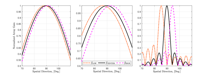
Figure 1: Normalized array gain with respect to spatial direction at low, center and high end subcarriers for (left) $f_{\mathrm{CENTER}}=3.5$ GHz, $B=0.1$ GHz; (middle) $f_{\mathrm{CENTER}}=28$ GHz, $B=2$ GHz; and (right) $f_{\mathrm{CENTER}}=300$ GHz, $B=30$ GHz, respectively.

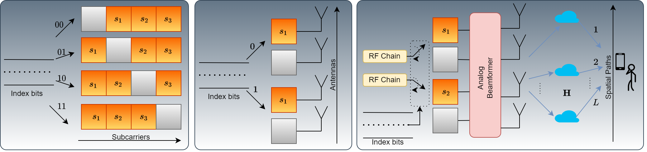
Figure 2: IM over subcarriers (left), antennas (middle), and spatial path indices (right).

Despite the cost-power benefits of hybrid analog/digital beamformers, they are limited in multiplexing gain [9, 10]. This is of particular concern for future wireless communications, where improved energy/spectral efficiency (EE/SE) is a key consideration [9]. Lately, index modulation (IM) has attracted interest as a means to achieve improved EE and SE than the conventional modulation schemes [17, 18]. In IM, the transmitter encodes additional information in the indices of the transmission media such as subcarriers [19] (SIM), antennas [20, 21, 22], and spatial paths [23, 24, 25, 26, 27, 28] (see Fig. 2). Since both antenna and path index modulation are performed in the spatial domain, we categorize these spatial modulation (SM) techniques as spatial antenna/path index modulation (SAIM/SPIM), respectively. In this paper, we focus on SPIM.

I-A Related Work

In [24], SPIM-based communication scenario was considered, wherein the indices of the spatial paths were modulated to create different spatial patterns for mmWave-MIMO. The same approach was exploited in [25] by employing lens arrays at both transmitter and receiver. In [27], a low-complexity approach was proposed for SPIM with a joint design of analog and digital beamformers. A similar architecture was also deployed for secure SAIM [29] and SPIM [30, 31] in the presence of eavesdropping users. Moreover, SE [23, 26] and EE [32] have been utilized as performance metrics for analog-only beamforming and receiver design. In order to extract the spatial paths for SM, a super-resolution channel estimation approach was proposed in [33]. In addition to the SM techniques employed over the antennas at the BS or communication user, SM over the reflecting surface elements has also been considered [21, 34, 35]. Different from the aforementioned model-based techniques, a machine learning based approach was also proposed in [36] for SPIM scenario. Furthermore, an SPIM-based MIMO system is experimented in [24].

Although there are several SM-based studies in the literature for communication-only systems, its usage for ISAC applications is relatively recent. For SM-aided ISAC systems, [22] devised a SAIM approach, wherein the antenna subarrays are allocated between different radar pulses and symbol time slots to handle sensing and communications tasks disjointly without mutual interference. This was further investigated in [37], which employed SM over antenna indices for orthogonal frequency division multiplexing (OFDM) ISAC, for which the OFDM carriers are divided into two groups and assigned exclusively to an active antenna to perform sensing and communications (S&C). In a more sensing-centric scenario, [38, 39] proposed a clutter suppression approach for ISAC based on the similarity of the generated spatial patterns. Also in [40], a low-complexity SAIM technique was proposed with one-bit analog-digital converters (ADCs). To sum up, the aforementioned ISAC works [22, 38, 39, 40, 37], consider only SM over antenna or subcarrier indices and do not exploit SPIM. On the other hand, the proposed SPIM approaches in [24, 25, 26, 23] consider the communications-only scenario without accounting for the trade-off between S&C functionalities (see Table I). Hybrid beamforming for THz-ISAC has been previously proposed in [4] with OFDM signaling.

TABLE I: Comparison With The State-of-The-Art

q.v.	mmWave	THz	Wideband	Beam-squint	SIM	SAIM	SPIM	ISAC
[24, 25, 26, 23, 27, 30, 31]	✓	$\times$	$\times$	$\times$	$\times$	$\times$	✓	$\times$
[19, 18]	✓	$\times$	✓	$\times$	✓	$\times$	$\times$	$\times$
[22, 38, 39, 40]	✓	$\times$	$\times$	$\times$	$\times$	$\times$	$\times$	✓
[29]	✓	$\times$	$\times$	$\times$	$\times$	✓	$\times$	$\times$
[37]	✓	$\times$	✓	$\times$	$\times$	✓	$\times$	✓
[40]	✓	$\times$	$\times$	$\times$	$\times$	$\times$	✓	$\times$
[4]	$\times$	✓	✓	✓	$\times$	$\times$	$\times$	✓
[41]	✓	$\times$	$\times$	$\times$	$\times$	$\times$	✓	✓
This paper	✓	✓	✓	✓	$\times$	$\times$	✓	✓

I-B Our Contributions

Contrary to the aforementioned studies, we leverage SPIM for mmWave and THz ISAC systems to achieve higher spectral efficiency. Preliminary results of our work appeared in our conference publication [41], where only a single target scenario was investigated for narrowband mmWave system. In this paper, we expand our study to include wideband THz-band systems, at which beam-split occurs. We also propose novel hybrid beamforming techniques to mitigate the impact of beam-split. Our proposed beamformer simultaneously maximizes the SE at the communications user over SPIM-aided signaling and achieves as much signal-to-noise ratio (SNR) as possible for detecting the radar targets. The SPIM-ISAC analog beamformer comprises radar-only and communications-only beamformers. While the former is constructed from the steering vectors corresponding to the target direction-of-arrivals (DoAs), the latter is selected from different spatial patterns between the BS and the communications user. The proposed design also includes a trade-off parameter between communications and radar sensing operations in the sense that the SNR at the targets and the user is controlled. In order to design the radar-only beamformer, the target DoAs are estimated during the search stage of the radar via wideband beam-split-aware (BSA) multiple signal classification (MUSIC) algorithm. Then, all possible spatial patterns between the BS and the user are exploited by estimating the wideband channel via the BSA orthogonal matching pursuit (BSA-OMP) algorithm [42], wherein SPIM is not considered. Thereafter, the hybrid beamformer is designed for each spatial pattern in accordance with the trade-off parameter. Note that the algorithms proposed in this work are also applicable to both narrow and wideband mmWave systems. Our main contributions in this paper are:

1. SPIM-ISAC: Despite the performance loss due to beam-split in wideband systems (especially in THz-band), our proposed SPIM-ISAC approach is particularly helpful to improve the SE via transmitting additional information bits. By exploiting the SPIM, our proposed approach surpasses even fully digital (FD) beamformer design, thereby exhibiting great potential for the next generation of S&C systems.

2. Beam-Split-Aware Algorithms: We introduce efficient approaches for wideband DoA/channel estimation and hybrid beamforming while simultaneously compensating the impact of beam-split without additional hardware components, e.g., TDs. The key idea of the proposed BSA approach is to exploit the angular deviations in the spatial domain due to beam-split. We then employ the MUSIC/OMP algorithm for DoA/channel estimation, which accounts for this deviation thereby ipso facto mitigating the effect of beam-split. To design the hybrid beamformers, unlike previous works relying on TD networks, we design an updated baseband beamformer, which handles the beam-split compensation in the baseband. Therefore, it does not require additional hardware and exhibits satisfactory performance.

3. Analog-Only and Hybrid Beamformers: We propose three different beamforming schemes: SD-analog-only (AO), SI-AO, and hybrid beamformers. All of these schemes have certain trade-offs. While the SD-AO beamformer can accurately compensate for the beam-split with high hardware complexity because of SD phase shifter networks, the SI-AO beamformer has simple architecture at the cost of lower SE. On the other hand, the proposed SPIM-ISAC hybrid beamformer takes advantage of employing a baseband beamformer with the proposed BSA beamforming technique to achieve higher SE than the AO beamformers with low hardware complexity.

I-C Notation

Throughout the paper, $(\cdot)^{\textsf{T}}$ and $(\cdot)^{\textsf{H}}$ denote the transpose and conjugate transpose operations, respectively. For a matrix $\mathbf{A}$ and vector $\mathbf{a}$; $[\mathbf{A}]_{ij}$, $[\mathbf{A}]_{k}$ and $[\mathbf{a}]_{l}$ correspond to the $(i,j)$-th entry, $k$-th column and $l$-th entry, respectively. $\lfloor\cdot\rfloor$ and $\mathbb{E}\{\cdot\}$ represent the flooring and expectation operations, respectively. The binomial coefficient is defined as $\footnotesize\left(\begin{array}[]{c}n\\ k\end{array}\right)=\frac{n!}{k!(n-k)!}$. An $N\times N$ identity matrix is represented by $\mathbf{I}_{N}$. The pulse-shaping function is represented by $\mathrm{sinc}(t)=\frac{\pi t}{t}$, $\xi(a)=\frac{\sin N\pi a}{N\sin\pi a}$ is the Dirichlet sinc function, and $\lceil\cdot\rceil$ denotes the ceiling operation. We denote $||\cdot||_{2}$ and $||\cdot||_{\mathcal{F}}$ as the $l_{2}$-norm and Frobenious norm, respectively.

II System Model

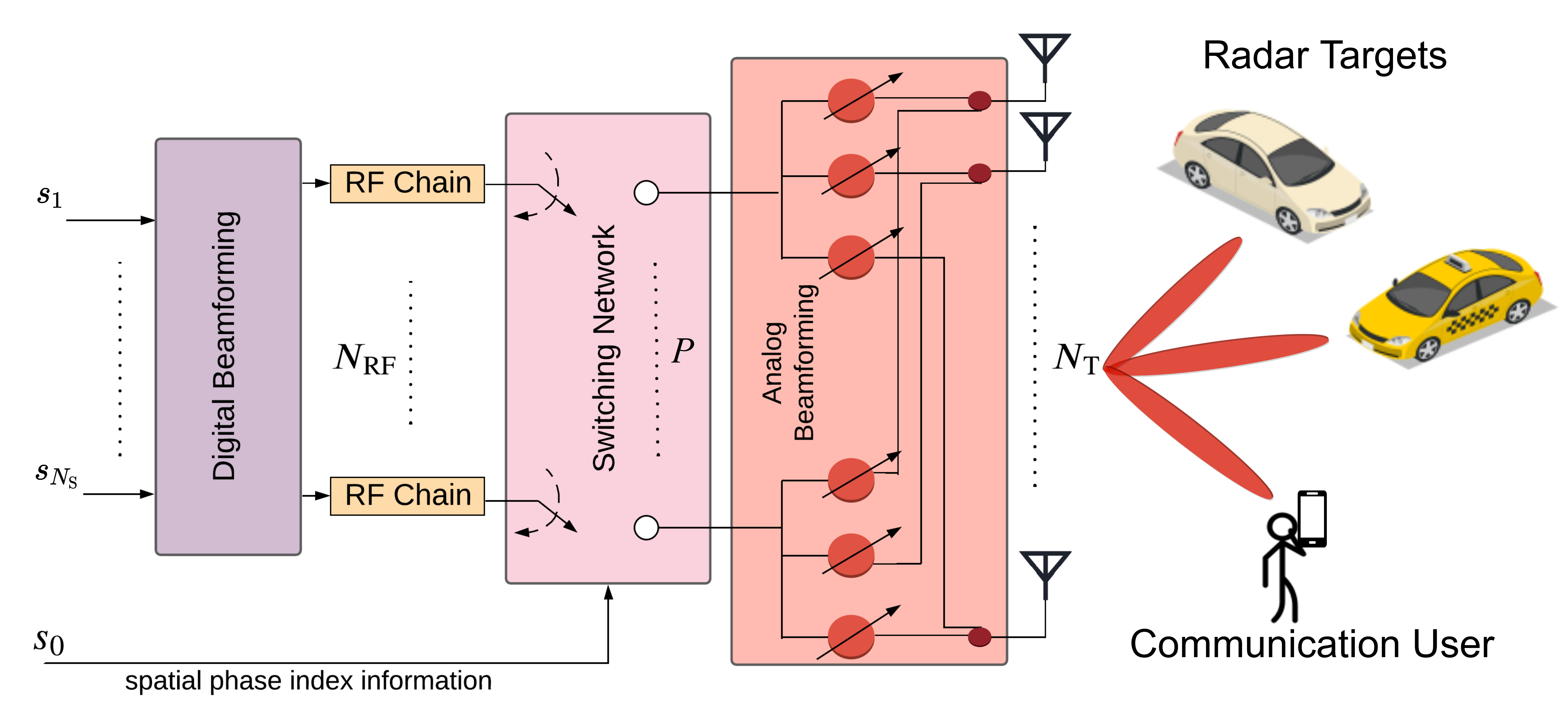
Figure 3: The SPIM-ISAC architecture processes the incoming data streams and employs spatial path index information $s_{0}$ in a switching network, which connects $N_{\mathrm{RF}}$ RF chains to $P=L+K$ taps on the analog beamformers to exploit $K$ paths for the radar targets and $L_{\mathrm{S}}$ out of $L$ spatial paths for the communications user.

Consider a wideband transmitter design problem in an ISAC scenario with SPIM involving a communications user and $K$ radar targets (Fig. 3). The dual-function BS employs $M$ subcarriers and it has $N_{\mathrm{T}}$ antennas to jointly communicate with the communication user and sense the radar targets via probing signals. The user has $N_{\mathrm{R}}$ antennas, for which $N_{\mathrm{S}}$ data symbols $\mathbf{s}[m]=[s_{1}[m],\cdots,s_{N_{\mathrm{S}}}[m]]^{\textsf{T}}\in\mathbb{C}^{N_{\mathrm{S}}}$ are transmitted, where $\mathbb{E}\{\mathbf{s}[m]\mathbf{s}^{\textsf{H}}[m]\}=\frac{1}{N_{\mathrm{S}}}\mathbf{I}_{N_{\mathrm{S}}}$. Additionally, the spatial path index information represented by ${s}_{0}$ is fed to the switching network (Fig. 3) to assign the outputs of $N_{\mathrm{RF}}$ RF chains to the $P$ taps of the analog beamformer. Here, $P$ is defined as the total number of spatial paths resolved at the BS from the targets and communications user as

$$P=L+K,$$ (1)

where $L$ and $K$ paths are reserved for communications and radar operations, respectively. We also define $L_{\mathrm{S}}$ as the selected number of paths out of $L$ total communication paths for SPIM. Thus, we have

$$N_{\mathrm{RF}}=L_{\mathrm{S}}+K,$$ (2)

which indicates that $L_{\mathrm{S}}$ columns of the analog beamformer are dedicated to communications task while the remaining $K$ columns are employed for sensing. As a result of this information-driven random switching with IM [17], there exist $\footnotesize\left(\begin{array}[]{c}L\\ Ls\end{array}\right)$ choices of connection to incorporate the spatial domain information as a principle of IM. Thus, the BS can process at most $P\geq N_{\mathrm{RF}}$ inputs, and each of the $P$ inputs is connected to the $N_{\mathrm{T}}>P$ BS antennas via phase shifters forming a fully-connected structure. The switching operation between the RF chains and the phase shifters needs to be performed in accordance with the symbol duration, for which low-cost switches with the speed of nanoseconds are available [28, 9].

In the extreme cases, such as $K=0$ (communications-only) and $L=0$ (sensing-only), the proposed ISAC approach can still work regardless of received paths from the user and targets. This can be done by adjusting the sensing-communications trade-off parameter defined in (42). It can also be seen that when $L_{\mathrm{S}}=L$, the proposed SPIM-ISAC configuration reduces to conventional ISAC system, regardless of $K$, since there is only a single choice of connection of transmission [23, 28]. Thus, compared to the conventional ISAC systems, the proposed SPIM-ISAC architecture has the advantage of transmitting additional data streams toward the communication user by exploiting the spatial pattern of the channel with limited RF chains, i.e., $N_{\mathrm{RF}}\leq P$ while performing radar sensing task with $K$ line-of-sight (LoS) spatial paths. Note also that the communication user requires $\bar{N}_{\mathrm{RF}}\geq L_{\mathrm{S}}$ RF chains in order to perform SPIM for processing $L_{\mathrm{S}}$ paths. Then, we define the total number of spatial patterns for communication as

$$S=2^{\left\lfloor\log_{2}\left(\footnotesize\begin{array}[]{c}L\\ L_{\mathrm{S}}\end{array}\right)\right\rfloor}.$$ (5)

II-A Communications Model

The BS aims to transmit the data symbol vector $\mathbf{s}[m]\in\mathbb{C}^{N_{\mathrm{S}}}$ toward the communications user. Thus, the BS first applies the SD baseband beamformer $\mathbf{F}_{\mathrm{BB}}^{(i)}[m]\in\mathbb{C}^{N_{\mathrm{RF}}\times N_{\mathrm{S}}}$ ($N_{\mathrm{S}}=L_{\mathrm{S}}$) for the $i$-th spatial pattern. Then, $M$-point inverse fast Fourier transform (IFFT) is applied to convert the signal to time-domain, and the cyclic prefix (CP) is added. Finally, the SI analog beamformer ${\mathbf{F}}_{\mathrm{RF}}^{(i)}\in\mathbb{C}^{N_{\mathrm{T}}\times N_{\mathrm{RF}}}$ is applied. Denoting the index set of possible spatial patterns by $\mathcal{S}=\{1,\cdots,S\}$, the $N_{\mathrm{T}}\times 1$ transmit signal for the $i$-th, ($i\in\mathcal{S}$), spatial pattern becomes

$$\mathbf{x}^{(i)}[m]=\mathbf{F}_{\mathrm{RF}}^{(i)}\mathbf{F}_{\mathrm{BB}}^{(i)}[m]\mathbf{s}[m],$$ (6)

where the analog beamformer $\mathbf{F}_{\mathrm{RF}}^{(i)}$ has constant-modulus constraint, i.e., $|[\mathbf{F}_{\mathrm{RF}}^{(i)}]_{n,r}|=1/\sqrt{N_{\mathrm{T}}}$ for $n=1,\cdots,N_{\mathrm{T}}$, $r=1,\cdots,N_{\mathrm{RF}}$. Further, we have $\sum_{m=1}^{M}\|\mathbf{F}_{\mathrm{RF}}^{(i)}\mathbf{F}_{\mathrm{BB}}^{(i)}[m]\|_{\mathcal{F}}^{2}=MN_{\mathrm{S}}$ to account for the total power constraint.

II-A1 Channel Model

In this study, we employ Saleh-Valenzuela (S-V) multipath channel model, which is the superposition of received non-LoS (NLoS) paths to model both mmWave and THz channel [43, 44, 11, 9]. Compared to the mmWave channel, the THz channel involves limited reflected paths and negligible scattering [43, 45]. For example, approximately $5$ paths survive at $0.3$ THz for THz massive MIMO systems as compared to approximately $8$ paths at $60$ GHz [45]. Especially for outdoor applications, multipath channel models are widely used to represent the THz channel for a more general scenario [43, 44, 45]. Hence, in this work, we consider a general scenario, wherein the delay-$\bar{d}$ $N_{\mathrm{R}}\times N_{\mathrm{T}}$ MIMO communications channel involving $L$ NLoS paths is given in discrete-time domain as

$$\tilde{\mathbf{H}}(\bar{d})=\sum_{l=1}^{L}{\gamma}_{l}\mathrm{sinc}(\bar{d}-B\tau_{l})\mathbf{a}_{\mathrm{R}}(\phi_{l})\mathbf{a}_{\mathrm{T}}^{\textsf{H}}(\theta_{l}),$$ (7)

where ${\gamma}_{l}\in\mathbb{C}$ denotes the channel path gain, $B$ represents the system bandwidth and $\tau_{l}$ is the time delay of the $l$-th path. $\phi_{l}$ and $\theta_{l}$ denote the physical DoA and direction-of-departure (DoD) angles of the scattering paths between the user and the BS, respectively, where $\phi_{l}=\sin\tilde{\phi}_{l}$, $\theta_{l}=\sin\tilde{\theta}_{l}$ and $\tilde{\phi}_{l},\tilde{\theta}_{l}\in[-\frac{\pi}{2},\frac{\pi}{2}]$. Then, the corresponding receive and transmit steering vectors are defined as $\mathbf{a}_{\mathrm{R}}(\phi_{l})\in\mathbb{C}^{N_{\mathrm{R}}}$ and $\mathbf{a}_{\mathrm{T}}(\theta_{l})\in\mathbb{C}^{N_{\mathrm{T}}}$, respectively. Performing $M$-point FFT of the delay-$\bar{d}$ channel given in (7) yields $\mathbf{H}[m]=\sum_{\bar{d}=1}^{\bar{D}-1}\tilde{\mathbf{H}}(\bar{d})e^{-\mathrm{j}\frac{2\pi m}{M}\bar{d}}$, where $\bar{D}\leq M$ is the CP length. Then, the $N_{\mathrm{R}}\times N_{\mathrm{T}}$ channel matrix in frequency domain is represented by

$$\mathbf{H}[m]=\sum_{l=1}^{L}{\gamma}_{l}\mathbf{a}_{\mathrm{R}}(\varphi_{l,m})\mathbf{a}_{\mathrm{T}}^{\textsf{H}}(\vartheta_{l,m})e^{-\mathrm{j}2\pi\tau_{l}f_{m}},$$ (8)

where $\varphi_{l,m}$ and $\vartheta_{l,m}$ denote the spatial directions, which are SD and they are deviated from the physical directions $\phi_{l}$, $\theta_{l}$ in the beamspace due to beam-split phenomenon. On the other hand, the beam-split-free channel matrix is $\overline{\mathbf{H}}[m]=\sum_{l=1}^{L}{\gamma}_{l}\mathbf{a}_{\mathrm{R}}(\phi_{l})\mathbf{a}_{\mathrm{T}}^{\textsf{H}}(\theta_{l})e^{-\mathrm{j}2\pi\tau_{l}f_{m}}$.

II-A2 Beam-Split Effect

In wideband transmission, a single wavelength assumption, i.e., $\lambda_{1}=\cdots\lambda_{M}=\frac{c_{0}}{f_{c}}$, is usually made across the subcarriers, where $c_{0}$ and $f_{c}$ are the speed of light and carrier frequency, respectively. However, due to employing a single analog beamformer, the single wavelength assumption does not hold, and the generated beams by employing a single analog beamformer split and point to different directions in the spatial domain [13, 2]. Suppose that similar beamforming architecture (i.e., SI analog beamformer with SD digital beamformers) is employed at the user. Then, the DoA angles at the user are also affected by beam-split. The relationship between the spatial ($\varphi_{l,m},\vartheta_{l,m}$) and the physical directions ($\phi_{l},\theta_{l}$) is given as

$$\varphi_{l,m}=\eta_{m}\phi_{l},\hskip 10.0pt\vartheta_{l,m}=\eta_{m}\theta_{l},$$ (9)

where $\eta_{m}=\frac{f_{m}}{f_{c}}$, $f_{m}=f_{c}+\frac{B}{M}(m-1-\frac{M-1}{2})$ is the $m$-th subcarrier frequency for the system bandwidth $B$. Notice that the beam-split is mitigated if the spatial $\varphi_{l,m},\vartheta_{l,m}$ and physical directions $\phi_{l},\theta_{l}$ are equal, i.e., $\eta_{m}=1$. This can be accomplished in the following ways:

1. $f_{m}\approx f_{c}$, which corresponds to the narrowband scenario where the carrier frequency is much larger than the system bandwidth (i.e. $f_{c}\gg B$).

2. Additional hardware components, e.g., TDs, (each of which consumes approximately $100$ mW [2, 15]) are employed between the phase shifters and the RF chains [14, 15] to compensate for the angular deviation in the generated beams due to beam-split via generating virtual SD analog beamformers.

3. The analog beamformers can be designed in an SD manner (see Sec. IV-C3), which can alleviate the effect of beam-split, at the cost of employing $MN_{\mathrm{T}}N_{\mathrm{RF}}$ (instead of $N_{\mathrm{T}}N_{\mathrm{RF}}$) phase-shifters (each of which consumes approximately $20$ mW at $60$ GHz ($40$ mW at $0.3$ THz) [2]).

4. Advanced signal processing techniques can be used to compensate for the beam-split via correcting the deviated phase terms of the analog beamformers (see Sec. IV-C2).

By considering a uniform linear array (ULA) configuration with $d=\frac{\lambda_{c}}{2}=\frac{c_{0}}{2f_{c}}$ half-wavelength element spacing, the $n$-th element of the beam-split-free transmit steering vector is $[\mathbf{a}_{\mathrm{T}}(\theta_{l})]_{n}=\frac{1}{N_{\mathrm{T}}}\exp\{-\mathrm{j}\pi(n-1)\theta_{l}\}$. However, under the effect of beam-split, the $n$-th entry of the SD steering vector $\mathbf{a}_{\mathrm{T}}(\vartheta_{l,m})$ is given by

$$[\mathbf{a}_{\mathrm{T}}(\vartheta_{l,m})]_{n} =\frac{1}{\sqrt{N_{\mathrm{T}}}}\exp\left\{-\mathrm{j}\frac{2\pi d}{\lambda_{m}}(n-1)\theta_{l}\right\}$$

$$=\frac{1}{\sqrt{N_{\mathrm{T}}}}\exp\left\{-\mathrm{j}\pi\frac{f_{m}}{f_{c}}(n-1)\theta_{l}\right\}$$

$$=\frac{1}{\sqrt{N_{\mathrm{T}}}}\exp\left\{-\mathrm{j}\pi(n-1)\eta_{m}\theta_{l}\right\},$$ (10)

where $\lambda_{m}=\frac{c_{0}}{f_{m}}$ is the wavelength of the $m$-th subcarrier. Note that $\eta_{m}=1$ in (10) yields no beam-split condition. The channel model in (8) is given in a compact form as

$$\mathbf{H}[m]=\mathbf{P}_{m}\boldsymbol{\Lambda}_{m}\mathbf{Q}_{m}^{\textsf{H}},$$ (11)

where the matrices $\mathbf{P}_{m}\in\mathbb{C}^{N_{\mathrm{R}}\times L}$ and $\mathbf{Q}_{m}\in\mathbb{C}^{N_{\mathrm{T}}\times L}$ represent the receive and transmit array responses for $L$ paths as $\mathbf{P}_{m}=[\mathbf{a}_{\mathrm{R}}(\varphi_{1,m}),\cdots,\mathbf{a}_{\mathrm{R}}(\varphi_{L,m})]$ and $\mathbf{Q}_{m}=[\mathbf{a}_{\mathrm{T}}(\vartheta_{1,m}),\cdots,\mathbf{a}_{\mathrm{T}}(\vartheta_{L,m})]$, respectively. $\boldsymbol{\Lambda}_{m}\in\mathbb{C}^{L\times L}$ is a diagonal matrix comprised of path gains ${\gamma}_{l}$ as $\boldsymbol{\Lambda}_{m}=\mathrm{diag}\{\tilde{\gamma}_{1},\cdots,\tilde{\gamma}_{L}\}$, where $\tilde{\gamma}_{l}={\gamma}_{l}e^{-\mathrm{j}2\pi\tau_{l}f_{m}}$ and ${\gamma}_{1}>{\gamma}_{2}>\cdots>{\gamma}_{L}$. Then, the $N_{\mathrm{R}}\times 1$ received signal at the communications user for the $i$-th spatial pattern is

$$\mathbf{y}^{(i)}[m]=\mathbf{H}[m]\mathbf{F}_{\mathrm{RF}}^{(i)}\mathbf{F}_{\mathrm{BB}}^{(i)}[m]\mathbf{s}[m]+\mathbf{n}[m],$$ (12)

where $\mathbf{n}[m]\sim\mathcal{CN}(\mathbf{0},\sigma_{n}^{2}\mathbf{I}_{N_{\mathrm{R}}})\in\mathbb{C}^{N_{\mathrm{R}}}$ represents the temporarily and spatially additive white Gaussian noise vector.

II-B Radar Model

The aim of the radar sensing task is to achieve the highest SNR toward target directions. Denote the estimate of the $k$-th target direction by $\Phi_{k}$ and select the radar-only beamformer as $\mathbf{F}_{\mathrm{R}}=[\mathbf{a}_{\mathrm{T}}(\Phi_{1}),\cdots,\mathbf{a}_{\mathrm{T}}(\Phi_{K})]\in\mathbb{C}^{N_{\mathrm{T}}\times K}$. Then, using the hybrid beamforming structure, the beampattern of the radar for $\Phi\in[-\frac{\pi}{2},\frac{\pi}{2}]$ is

$$B^{(i)}_{m}(\Phi)=\mathrm{Trace}\{\mathbf{a}_{\mathrm{T}}(\Phi)^{\textsf{H}}(\Phi)\mathbf{R}_{\mathbf{x}}^{(i)}[m]\mathbf{a}_{\mathrm{T}}(\Phi)\},$$ (13)

where $\mathbf{a}_{\mathrm{T}}(\Phi)\in\mathbb{C}^{N_{\mathrm{T}}}$ denotes the steering vector corresponding arbitrary target direction $\Phi$, and $\mathbf{R}_{\mathbf{x}}^{(i)}[m]\in\mathbb{C}^{N_{\mathrm{T}}\times N_{\mathrm{T}}}$ is the covariance of the transmit signal. For the $i$-th spatial pattern, we have

$$\mathbf{R}_{\mathbf{x}}^{(i)}[m] =\mathbb{E}\{\mathbf{x}^{(i)}[m]\mathbf{x}^{(i)^{\textsf{H}}}[m]\}$$

$$=\mathbb{E}\{\mathbf{F}_{\mathrm{RF}}^{(i)}\mathbf{F}_{\mathrm{BB}}^{(i)}[m]\mathbf{s}[m]\mathbf{s}^{\textsf{H}}[m]\mathbf{F}_{\mathrm{BB}}^{(i)^{\textsf{H}}}[m]\mathbf{F}_{\mathrm{RF}}^{(i)^{\textsf{H}}}\}$$

$$=\mathbf{F}_{\mathrm{RF}}^{(i)}\mathbf{F}_{\mathrm{BB}}^{(i)}[m]\mathbb{E}\{\mathbf{s}[m]\mathbf{s}^{\textsf{H}}[m]\}\mathbf{F}_{\mathrm{BB}}^{(i)^{\textsf{H}}}[m]\mathbf{F}_{\mathrm{RF}}^{(i)^{\textsf{H}}}$$

$$=\frac{1}{N_{\mathrm{S}}}\mathbf{F}_{\mathrm{RF}}^{(i)}\mathbf{F}_{\mathrm{BB}}^{(i)}[m]\mathbf{F}_{\mathrm{BB}}^{(i)^{\textsf{H}}}[m]\mathbf{F}_{\mathrm{RF}}^{(i)^{\textsf{H}}}.$$ (14)

To simultaneously obtain the desired beampattern for the radar target and provide satisfactory communications performance, the hybrid beamformer $\mathbf{F}_{\mathrm{RF}}^{(i)}\mathbf{F}_{\mathrm{BB}}^{(i)}[m]$ should be designed accordingly.

III Problem Formulation

In order to design SPIM-ISAC hybrid beamformers, we aim to maximize the SE, which is characterized by the mutual information (MI). Therefore, in what follows, we first introduce the SE expression of both SPIM- assisted and conventional systems.

III-A SE of the SPIM-ISAC System

Define $\mathrm{SE}(\mathbf{y}^{(i)}[m];\mathbf{x}^{(i)}[m],\mathbf{F}^{(i)}[m])$ as the MI of the overall wireless transmission for the received and transmitted signals $\mathbf{y}^{(i)}[m]$ and $\mathbf{x}^{(i)}[m]$ at the $i$-th spatial pattern with the hybrid beamformer $\mathbf{F}^{(i)}[m]=\mathbf{F}_{\mathrm{RF}}^{(i)}\mathbf{F}_{\mathrm{BB}}^{(i)}[m]$. Then, $\mathrm{SE}(\mathbf{y}^{(i)}[m];\mathbf{x}^{(i)}[m],\mathbf{F}^{(i)}[m])$ is defined as

$$\mathrm{SE}(\mathbf{y}^{(i)}[m];\mathbf{x}^{(i)}[m],\mathbf{F}^{(i)}[m])=\mathrm{SE}(\mathbf{y}^{(i)}[m];\mathbf{x}^{(i)}[m]|\mathbf{F}^{(i)}[m])$$

$$\hskip 70.0pt+\mathrm{SE}(\mathbf{y}^{(i)}[m];\mathbf{F}^{(i)}[m]),\hskip 10.0ptm\in\mathcal{M},$$ (15)

where $\mathrm{SE}(\mathbf{y}^{(i)}[m];\mathbf{x}^{(i)}[m]|\mathbf{F}^{(i)}[m])$ and $\mathrm{SE}(\mathbf{y}^{(i)}[m];\mathbf{F}^{(i)}[m])$ stand for the MI corresponding to conventional symbol transmission and the MI achieved by employing SPIM, respectively. In particular, $\mathrm{SE}(\mathbf{y}^{(i)}[m];\mathbf{x}^{(i)}[m]|\mathbf{F}^{(i)}[m])$ is well-known [9] as

$$\mathrm{SE}(\mathbf{y}^{(i)}[m];\mathbf{x}^{(i)}[m]|\mathbf{F}^{(i)}[m])=\frac{1}{S}\sum_{i=1}^{S}\log_{2}\mathrm{det}\{\boldsymbol{\Sigma}_{i}[m]\},$$ (16)

where $\boldsymbol{\Sigma}_{i}[m]=\mathbf{I}_{N_{\mathrm{R}}}+\frac{1}{\sigma_{n}^{2}N_{\mathrm{S}}}\mathbf{H}[m]\mathbf{F}^{(i)}[m]{\mathbf{F}^{(i)}}^{\textsf{H}}[m]\mathbf{H}^{\textsf{H}}[m].$

While there is no closed-form expression for $\mathrm{SE}(\mathbf{y}^{(i)}[m];\mathbf{F}^{(i)}[m])$, it is lower-bounded by $\mathrm{SE}_{\mathrm{LB}}(\mathbf{y}^{(i)}[m];\mathbf{F}^{(i)}[m])$ [23], which is

$$\mathrm{SE}_{\mathrm{LB}}(\mathbf{y}^{(i)}[m];\mathbf{F}^{(i)}[m])=\log_{2}S-N_{\mathrm{R}}\log_{2}e$$

$$\hskip 30.0pt-\frac{1}{S}\sum_{i=1}^{S}\log_{2}\left(\sum_{j=1}^{S}\frac{\mathrm{det}\{\boldsymbol{\Sigma}_{i}[m]\}}{\mathrm{det}\{\boldsymbol{\Sigma}_{i}[m]+\boldsymbol{\Sigma}_{j}[m]\}}\right).$$ (17)

Combining (16) and (17), we obtain the SE of the SPIM-aided system as

$$\mathrm{SE}_{\mathrm{SPIM}}[m]=\log_{2}\left(\frac{S}{(2\sigma_{n}^{2})^{N_{\mathrm{R}}}}\right)$$

$$\hskip 20.0pt-\frac{1}{S}\sum_{i=1}^{S}\log_{2}\left(\sum_{j=1}^{S}\mathrm{det}\{\boldsymbol{\Sigma}_{i}[m]+\boldsymbol{\Sigma}_{j}[m]\}^{-1}\right).$$ (18)

III-B SE of the MIMO-ISAC System

In conventional MIMO systems, the analog beamformer ${\mathbf{F}}_{\mathrm{RF}}$ relies on the selection of the strongest path for hybrid beamformer design [28, 23]. The SE expression is also the same for MIMO-ISAC. As an example, we have $\mathbf{F}_{\mathrm{RF}}^{(1)}=[\mathbf{F}_{\mathrm{R}},\mathbf{a}_{\mathrm{T}}(\theta_{1})]$, where $\mathbf{a}_{\mathrm{T}}(\theta_{1})$ corresponds to the strongest communications path with path gain ${\gamma}_{1}$. Since there is a one choice of transmission, i.e., $S=1$, the SE for MIMO-ISAC system is computed as

$$\mathrm{SE}_{\mathrm{MIMO}}[m]=\log_{2}\bigg{(}\mathrm{det}\bigg{\{}\mathbf{I}_{N_{\mathrm{R}}}$$

$$+\frac{1}{\sigma_{n}^{2}N_{\mathrm{S}}}\mathbf{H}[m]{\mathbf{F}}_{\mathrm{RF}}^{(1)}{\mathbf{F}}_{\mathrm{BB}}^{(1)}[m]{\mathbf{F}_{\mathrm{BB}}^{(1)}}^{\textsf{H}}[m]{\mathbf{F}_{\mathrm{RF}}^{(1)}}^{\textsf{H}}\mathbf{H}^{\textsf{H}}[m]\bigg{\}}\bigg{)},$$ (19)

where $i=1$ denotes the first spatial pattern which, in this case, corresponds to the path with strongest gain.

III-C Hybrid Beamformer Design

The SPIM-ISAC hybrid beamformer design problem is

$$\operatorname*{maximize}_{\mathbf{F}_{\mathrm{RF}}^{(i)},\{\mathbf{F}_{\mathrm{BB}}^{(i)}[m]\}_{m=1}^{M}} \sum_{m=1}^{M}\mathrm{SE}_{\mathrm{SPIM}}[m]$$

$$\operatorname*{subject\hskip 3.0ptto:\hskip 3.0pt}\hskip 10.0pt \mathbf{F}_{\mathrm{RF}}^{(i)}\in\mathcal{A},$$

$$|[\mathbf{F}_{\mathrm{RF}}^{(i)}]_{n,r}|=1/\sqrt{N_{\mathrm{T}}},\|\mathbf{F}_{\mathrm{RF}}^{(i)}\mathbf{F}_{\mathrm{BB}}^{(i)}[m]\|_{\mathcal{F}}=MN_{\mathrm{S}},$$ (20)

where $\mathbf{F}_{\mathrm{RF}}^{(i)}$ is a member of $\mathcal{A}=\{\mathbf{F}_{\mathrm{RF}}^{(1)},\cdots,\mathbf{F}_{\mathrm{RF}}^{(S)}\}$, which represents the set of possible analog beamformers for the SPIM. (III-C) also includes constraints for the constant-modulus property of $\mathbf{F}_{\mathrm{RF}}^{(i)}$ and the total power constraint.

The optimization problem in (III-C) falls to the class of mixed-integer non-convex programming (MINCP). In particular, it is computationally prohibitive because of the combinatorial subproblems for each spatial pattern $i$, and non-linear due to multiple unknowns $\mathbf{F}_{\mathrm{RF}}^{(i)}$ and $\mathbf{F}_{\mathrm{BB}}^{(i)}[m]$. In order to provide an effective beamforming solution, we exploit the steering vectors corresponding to the radar and communications paths to design the beamformers for SPIM-ISAC in the following.

IV SPIM in ISAC

Instead of solving (III-C), we utilize the radar and communications parameters to construct the analog and digital beamformers. In particular, the analog beamformer is constructed from the steering vectors corresponding to the directions of the radar targets and communications user paths. Thus, we define the analog beamformer $\mathbf{F}_{\mathrm{RF}}^{(i)}\in\mathbb{C}^{N_{\mathrm{T}}\times N_{\mathrm{RF}}}$ as

$$\mathbf{F}_{\mathrm{RF}}^{(i)}=\left[\mathbf{F}_{\mathrm{R}}\;|\;\mathbf{F}_{\mathrm{C}}^{(i)}\right],$$ (21)

where $\mathbf{F}_{\mathrm{C}}^{(i)}\in\mathbb{C}^{N_{\mathrm{T}}\times N_{\mathrm{S}}}$ is the communications-only analog beamformer comprised of the steering vectors corresponding to the communications paths for the $i$-th spatial pattern.

In the following, we first discuss the radar (i.e., target directions to construct $\mathbf{F}_{\mathrm{R}}$) and communication (i.e, $\mathbf{Q}_{m}$, $\mathbf{P}_{m}$ and $\boldsymbol{\Lambda}_{m}$ to construct ${\mathbf{F}}_{\mathrm{C}}^{(i)}$) parameter estimation. Then, we introduce the proposed hybrid beamforming technique for SPIM-ISAC.

IV-A Radar Parameter Estimation

The radar-only beamformer $\mathbf{F}_{\mathrm{R}}$ is constructed as the steering matrix corresponding to $\Phi_{k}$, $\forall k$, which are estimated during the search phase of the radar [4]. Toward this end, the BS first transmits probing signals, which are reflected and processed by the BS to estimate the target directions.

Define $\tilde{\mathbf{X}}_{\mathrm{r}}[m]\in\mathbb{C}^{N_{\mathrm{T}}\times T}$ as the radar probing signal transmitted by the BS for $T$ data snapshots along the fast-time axis [46, 3]. $\tilde{\mathbf{X}}_{\mathrm{r}}[m]$ has the property $\mathbb{E}\{\tilde{\mathbf{X}}_{\mathrm{r}}[m]\tilde{\mathbf{X}}_{\mathrm{r}}^{\textsf{H}}[m]\}=\frac{P_{\mathrm{r}}T}{MN_{\mathrm{T}}}\mathbf{I}_{N_{\mathrm{T}}}$, where $P_{\mathrm{r}}$ is the radar transmit power. The $N_{\mathrm{RF}}\times T$ echo signal reflected from the $K$ targets is

$$\tilde{\mathbf{Y}}[m]=\sum_{k=1}^{K}\beta_{k}\tilde{\mathbf{a}}_{\mathrm{T}}(\Phi_{k})\mathbf{a}_{\mathrm{T}}^{\textsf{T}}(\Phi_{k})\tilde{\mathbf{X}}_{\mathrm{r}}[m]+\tilde{\mathbf{N}}[m],$$ (22)

where $\beta_{k}\in\mathbb{C}$ denotes the reflection coefficient of the $k$-th target, $\mathbf{a}_{\mathrm{T}}(\Phi_{k})\in\mathbb{C}^{N_{\mathrm{T}}}$ is the transmit array steering vector corresponding to the $k$-th target DoA angle $\Phi_{k}$ and $\tilde{\mathbf{a}}_{\mathrm{T}}(\Phi_{k})=\mathbf{W}_{\mathrm{RF}}^{\textsf{H}}{\mathbf{a}}_{\mathrm{T}}(\Phi_{k})\in\mathbb{C}^{N_{\mathrm{RF}}}$ is the equivalent receive steering vector for $\mathbf{W}_{\mathrm{RF}}\in\mathbb{C}^{N_{\mathrm{T}}\times N_{\mathrm{RF}}}$ being the analog combiner matrix [3]. $\tilde{\mathbf{N}}[m]=\mathbf{W}_{\mathrm{RF}}^{\textsf{H}}\bar{\mathbf{N}}[m]\in\mathbb{C}^{N_{\mathrm{RF}}\times T}$ is representing the noise term, where $\bar{\mathbf{N}}[m]=[\bar{\mathbf{n}}_{1}[m],\cdots,\bar{\mathbf{n}}_{T}[m]]\in\mathbb{C}^{N_{\mathrm{T}}\times T}$ with $\bar{\mathbf{n}}_{t}[m]\sim\mathcal{CN}(\mathbf{0},\tilde{\sigma}_{n}^{2}\mathbf{I}_{N_{\mathrm{T}}})$. Denote the radar target steering matrix and reflection coefficients by $\tilde{\mathbf{A}}_{\mathrm{T}}(\Phi)=[\tilde{\mathbf{a}}_{\mathrm{T}}(\Phi_{1}),\cdots,\tilde{\mathbf{a}}_{\mathrm{T}}(\Phi_{K})]$ and $\boldsymbol{\Xi}=\mathrm{diag}\{\beta_{1},\cdots,\beta_{K}\}\in\mathbb{C}^{K\times K}$, then (22) becomes

$$\tilde{\mathbf{Y}}[m]=\tilde{\mathbf{A}}_{\mathrm{T}}(\Phi)\boldsymbol{\Xi}\mathbf{A}_{\mathrm{T}}^{\textsf{T}}(\Phi)\tilde{\mathbf{X}}_{\mathrm{r}}[m]+\tilde{\mathbf{N}}[m].$$ (23)

In order to estimate the target directions, we invoke the wideband MUSIC algorithm [47, 48]. Define $\mathbf{R}_{\tilde{\mathbf{Y}}}[m]\in\mathbb{C}^{N_{\mathrm{RF}}\times N_{\mathrm{RF}}}$ as the covariance matrix of $\tilde{\mathbf{Y}}[m]$, i.e.,

$$\mathbf{R}_{\tilde{\mathbf{Y}}}[m] =\frac{1}{T}\tilde{\mathbf{Y}}[m]\tilde{\mathbf{Y}}^{\textsf{H}}[m]$$

$$=\frac{1}{T}\tilde{\mathbf{A}}_{\mathrm{T}}(\Phi)\left(\frac{P_{\mathrm{r}}T}{MN_{\mathrm{T}}}\widetilde{\boldsymbol{\Xi}}\right)\tilde{\mathbf{A}}_{\mathrm{T}}^{\textsf{H}}(\Phi)+\frac{1}{T}\tilde{\mathbf{N}}[m]\tilde{\mathbf{N}}^{\textsf{H}}[m]$$

$$\approx\frac{P_{\mathrm{r}}}{MN_{\mathrm{T}}}\tilde{\mathbf{A}}_{\mathrm{T}}(\Phi)\widetilde{\boldsymbol{\Xi}}\tilde{\mathbf{A}}_{\mathrm{T}}^{\textsf{H}}(\Phi)+\tilde{\sigma}_{n}^{2}N_{\mathrm{T}}\mathbf{I}_{\mathrm{N}_{\mathrm{RF}}},$$ (24)

where $\tilde{\mathbf{N}}[m]\tilde{\mathbf{N}}^{\textsf{H}}[m]=\tilde{\sigma}_{n}^{2}T\mathbf{W}_{\mathrm{RF}}^{\textsf{H}}\mathbf{W}_{\mathrm{RF}}\approx\tilde{\sigma}_{n}^{2}TN_{\mathrm{T}}\mathbf{I}_{N_{\mathrm{RF}}}$ and $\widetilde{\boldsymbol{\Xi}}\in\mathbb{C}^{K\times K}$ is defined as $\widetilde{\boldsymbol{\Xi}}=\boldsymbol{\Xi}\mathbf{A}_{\mathrm{T}}^{\textsf{T}}(\Phi)\mathbf{A}_{\mathrm{T}}^{*}(\Phi)\boldsymbol{\Xi}^{*}$. Then, the eigendecomposition of $\mathbf{R}_{\tilde{\mathbf{Y}}}[m]$ yields

$$\mathbf{R}_{\tilde{\mathbf{Y}}}[m]=\mathbf{U}[m]\boldsymbol{\Theta}[m]\mathbf{U}^{\textsf{H}}[m],$$ (25)

where $\boldsymbol{\Theta}[m]\in\mathbb{C}^{N_{\mathrm{RF}}\times N_{\mathrm{RF}}}$ is a diagonal matrix composed of the eigenvalues of $\mathbf{R}_{\tilde{\mathbf{Y}}}[m]$ in a descending order, and $\mathbf{U}[m]=\left[\mathbf{U}_{\mathrm{S}}[m]\hskip 2.0pt\mathbf{U}_{\mathrm{N}}[m]\right]\in\mathbb{C}^{N_{\mathrm{RF}}\times N_{\mathrm{RF}}}$ corresponds to the eigenvector matrix; $\mathbf{U}_{\mathrm{S}}[m]\in\mathbb{C}^{N_{\mathrm{RF}}\times K}$ and $\mathbf{U}_{\mathrm{N}}[m]\in\mathbb{C}^{N_{\mathrm{RF}}\times N_{\mathrm{RF}}-K}$ are the signal and noise subspace eigenvector matrices, respectively. The columns of $\mathbf{U}_{\mathrm{S}}[m]$ and $\tilde{\mathbf{A}}_{\mathrm{T}}(\Phi)$ span the same space that is orthogonal to the eigenvectors in $\mathbf{U}_{\mathrm{N}}[m]$ as

$$\|\mathbf{U}_{\mathrm{N}}^{\textsf{H}}[m]\tilde{\mathbf{a}}_{\mathrm{T}}(\Phi_{k})\|_{2}^{2}=0,$$ (26)

for $k\in\mathcal{K}$ and $m\in\mathcal{M}$ [47]. Thus, the estimates of the radar targets can be founds from the combined MUSIC spectra, i.e.,

$$\zeta(\Phi)=\sum_{m=1}^{M}\zeta_{m}(\Phi),$$ (27)

where $\zeta_{m}(\Phi)$ is the spectrum corresponding to the $m$-th subcarrier as $\zeta_{m}(\Phi)=\frac{1}{\mathbf{a}_{\mathrm{T}}^{\textsf{H}}(\Phi)\mathbf{U}_{\mathrm{N}}[m]\mathbf{U}_{\mathrm{N}}^{\textsf{H}}[m]\mathbf{a}_{\mathrm{T}}(\Phi)}.$

The MUSIC spectra in (27) yields $MK$ peaks, which are deviated due to beam-split while correct MUSIC spectra should include $K$ peaks which are aligned for $m\in\mathcal{M}$. In other words, beam-split-corrected steering vectors should be used to accurately compute the MUSIC spectrum. Therefore, we propose the BSA-MUSIC algorithm, in which beam-split-corrected steering vectors are employed for the computation of the MUSIC spectrum.

Define $\mathbf{a}_{\mathrm{T}}(\Phi_{m})\in\mathbb{C}^{N_{\mathrm{T}}}$ as the BSA SD steering vector for the nominal SI steering vector $\mathbf{a}_{\mathrm{T}}(\Phi)$. The $n$-th entry of the BSA steering vector is explicitly defined as $[\mathbf{a}_{\mathrm{T}}(\Phi_{m})]_{n}=\frac{1}{\sqrt{N_{\mathrm{T}}}}\exp\{-\mathrm{j}\pi(n-1)\Phi_{m}\}$ whereas $[\mathbf{a}_{\mathrm{T}}(\Phi)]_{n}=\frac{1}{\sqrt{N_{\mathrm{T}}}}\exp\{-\mathrm{j}\frac{2\pi d}{\lambda_{m}}(n-1)\Phi\}$. The beam-split correction implies that $\mathbf{a}_{\mathrm{T}}(\Phi)=\mathbf{a}_{\mathrm{T}}(\Phi_{m})$ holds, such that while the frequency $f_{m}$ varies, $\mathbf{a}_{\mathrm{T}}(\Phi_{m})$ points to $\Phi$, whereas $\mathbf{a}_{\mathrm{T}}(\Phi)$ points to $\eta_{m}\Phi$. In other words, we have

$${[\mathbf{a}_{\mathrm{T}}(\Phi_{m})]_{n}}-{[\mathbf{a}_{\mathrm{T}}(\Phi)]_{n}} =0$$

$${\frac{1}{\sqrt{N_{\mathrm{T}}}}e^{-\mathrm{j}(n-1)\Phi_{m}}}-{\frac{1}{\sqrt{N_{\mathrm{T}}}}e^{-\mathrm{j}\frac{2\pi\frac{\lambda_{c}}{2}}{\lambda_{m}}(n-1)\Phi}} =0$$

$${e^{-\mathrm{j}\pi(n-1)\Phi_{m}}}-{e^{-\mathrm{j}\pi\frac{\lambda_{c}}{\lambda_{m}}(n-1)\Phi}} =0,$$ (28)

which yields $\Phi_{m}=\frac{\lambda_{c}}{\lambda_{m}}\Phi=\eta_{m}\Phi$.

To provide further insight, we examine the array gain, which also holds for computing the MUSIC spectrum [47], for wideband scenario in the following lemma, for which we define the array gain $A_{G}(\Phi,m)$ for $\Phi$ at the $m$-th subcarrier as

$$A_{G}(\Phi,m)=\frac{|\mathbf{a}_{\mathrm{T}}^{\textsf{H}}(\Phi)\mathbf{a}_{\mathrm{T}}(\Phi_{m})|^{2}}{N_{\mathrm{T}}^{2}}.$$ (29)

Lemma 1.

Let $\mathbf{a}_{\mathrm{T}}(\Phi_{m})$ and $\mathbf{a}_{\mathrm{T}}(\Phi)$ be the BSA and nominal steering vectors for an arbitrary direction $\Phi$ and subcarrier $m\in\mathcal{M}$ as defined in (28), respectively. Then, $\mathbf{a}_{\mathrm{T}}(\Phi_{m})$ achieves the maximum array gain, i.e., $A_{G}(\Phi,m)=\frac{|\mathbf{a}_{\mathrm{T}}^{\textsf{H}}(\Phi)\mathbf{a}_{\mathrm{T}}(\Phi_{m})|^{2}}{N_{\mathrm{T}}^{2}}$, if $\Phi_{m}=\eta_{m}\Phi$.

Proof.

Please see Appendix A. ∎

Using the aforementioned analysis and Lemma 1, the BSA-MUSIC spectrum is $\widetilde{\zeta}(\Phi)=\sum_{m=1}^{M}\widetilde{\zeta}_{m}(\Phi),$ where

$$\widetilde{\zeta}_{m}(\Phi)=\frac{1}{\boldsymbol{a}_{m}^{\textsf{H}}(\Phi)\mathbf{U}_{\mathrm{N}}[m]\mathbf{U}_{\mathrm{N}}^{\textsf{H}}[m]\boldsymbol{a}_{m}(\Phi)},$$ (30)

where $\boldsymbol{a}_{m}(\Phi)=\mathbf{W}_{\mathrm{RF}}^{\textsf{H}}\mathbf{a}_{\mathrm{T}}(\Phi_{m})\in\mathbb{C}^{N_{\mathrm{RF}}}$ denotes the beam-split-corrected virtual steering vector. The $K$ highest peaks of the BSA-MUSIC spectrum in (30) yields the radar target estimates $\{\hat{\Phi}_{k}\}_{k=1}^{K}$.

Remark 1: Since there are limited number of RF chains, the size of the collected array data in (22) for the MUSIC algorithm is $N_{\mathrm{RF}}\times T$, which allows us to identify $K\leq N_{\mathrm{RF}}-1$ targets. In order to improve the identifiability condition, full array data can be collected via subarray processing. In other words, the array data can be collected at multiple time slots, say $T_{\mathrm{slot}}=N_{\mathrm{T}}/N_{\mathrm{RF}}$ provided that the phase alignment between the time slots is properly handled [49]. Then, the echo signal in (22) is collected in $T_{\mathrm{slot}}$ time slots and the $N_{\mathrm{T}}\times T$ array data is constructed as

$$\widetilde{\mathbf{Y}}[m]=[\tilde{\mathbf{Y}}_{1}^{\textsf{T}}[m],\cdots,\tilde{\mathbf{Y}}_{T_{\mathrm{slot}}}^{\textsf{T}}[m]]^{\textsf{T}}\in\mathbb{C}^{N_{\mathrm{T}}\times T},$$ (31)

for which the identifiability condition is $K\leq N_{\mathrm{T}}-1$.

IV-B Communications Parameter Estimation

The communications-only analog beamformer ${\mathbf{F}}_{\mathrm{C}}^{(i)}$ is constructed from steering vectors corresponding to the path directions $\{\vartheta_{l}\}_{l=1}^{L}$. This can be done by the communication user feeding back $\{\vartheta_{l}\}_{l=1}^{L}$ to the BS after the channel acquisition stage at the user side.

In order to estimate the channel ${\mathbf{H}}[m]$, and eventually $\{\vartheta_{l}\}_{l=1}^{L}$, we employ an OMP-based approach relying on a BSA dictionary. The key idea of the proposed BSA dictionary is to utilize the prior knowledge of $\eta_{m}$ to obtain beam-split-corrected steering vectors. Thus, a BSA dictionary is constructed, wherein the steering vectors are generated with the directions that are affected by beam-split. Then, the physical direction can readily be found as $\phi=\frac{\varphi_{m}}{\eta_{m}}$, $\theta=\frac{\vartheta_{m}}{\eta_{m}}$ for an arbitrary spatial direction $\varphi_{m},\vartheta_{m}\in[-1,1]$, $\forall m\in\mathcal{M}$. Using this observation, we design the BSA dictionaries $\overline{\mathbf{P}}_{m}\in\mathbb{C}^{N_{\mathrm{R}}\times G}$ and $\overline{\mathbf{Q}}_{m}\in\mathbb{C}^{N_{\mathrm{T}}\times G}$, where $G$ is the grid size. Then, we have

$$\overline{\mathbf{P}}_{m} =[{\mathbf{a}}_{\mathrm{R}}(\varphi_{1,m}),\cdots,{\mathbf{a}_{\mathrm{R}}}(\varphi_{G,m})],$$ (32)

$$\overline{\mathbf{Q}}_{m} =[\mathbf{a}_{\mathrm{T}}(\vartheta_{1,m}),\cdots,\mathbf{a}_{\mathrm{T}}(\vartheta_{G,m})],$$ (33)

where $\mathbf{a}_{\mathrm{R}}(\varphi_{g,m})$ and $\mathbf{a}_{\mathrm{T}}(\vartheta_{g,m})$ are $N_{\mathrm{R}}\times 1$ and $N_{\mathrm{T}}\times 1$ steering vectors for $g=1,\cdots,G$.

In order to estimate the channel in downlink, the BS employs $J_{\mathrm{T}}$ beamformer vectors as $\tilde{\mathbf{F}}=[\tilde{\mathbf{f}}_{1},\cdots,\tilde{\mathbf{f}}_{J_{\mathrm{T}}}]\in\mathbb{C}^{N_{\mathrm{T}}\times{J_{\mathrm{T}}}}$ to transmit ${J_{\mathrm{T}}}$ orthogonal pilots, $\tilde{\mathbf{S}}[m]=\mathrm{diag}\{\tilde{s}_{1}[m],\cdots,\tilde{s}_{J_{\mathrm{T}}}[m]\}\in\mathbb{C}^{{J_{\mathrm{T}}}\times{J_{\mathrm{T}}}}$. For the transmit pilots corresponding to each $\tilde{\mathbf{f}}_{j}$, the user with $\bar{N}_{\mathrm{RF}}$ RF chain employs ${J_{\mathrm{R}}}$ ($J_{\mathrm{R}}\leq N_{\mathrm{R}}$) combining vectors $\tilde{\mathbf{w}}_{j}$ as $\tilde{\mathbf{W}}=[\tilde{\mathbf{w}}_{1},\cdots,\tilde{\mathbf{w}}_{{J_{\mathrm{R}}}}]\in\mathbb{C}^{N_{\mathrm{R}}\times{J_{\mathrm{R}}}}$. Therefore, the total channel usage for processing all pilots during training is $J_{\mathrm{T}}\lceil\frac{{J_{\mathrm{R}}}}{\bar{{N}}_{\mathrm{RF}}}\rceil$. At the user side, the received ${J_{\mathrm{R}}}\times{J_{\mathrm{T}}}$ signal is

$${\mathbf{Y}}[m]=\tilde{\mathbf{W}}^{\textsf{H}}\mathbf{H}[m]\tilde{\mathbf{F}}\tilde{\mathbf{S}}+\tilde{\mathbf{E}}[m],$$ (34)

where ${\mathbf{E}}[m]=\tilde{\mathbf{W}}^{\textsf{H}}\mathbf{N}[m]$ corresponds to the effective noise term. Assuming $\tilde{\mathbf{S}}[m]=\mathbf{I}_{J_{\mathrm{T}}}$, $\forall m\in\mathcal{M}$, we get

$${\mathbf{Y}}[m]=\tilde{\mathbf{W}}^{\textsf{H}}\mathbf{H}[m]\tilde{\mathbf{F}}[m]+{\mathbf{E}}[m],$$ (35)

which is rewritten in vector form as

$$\mathbf{y}[m]=(\tilde{\mathbf{F}}^{\textsf{T}}\otimes\tilde{\mathbf{W}}^{\textsf{H}})\mathbf{h}[m]+{\mathbf{e}}[m],$$ (36)

where $\mathbf{y}[m]=\mathrm{vec}\{{\mathbf{Y}}[m]\}\in\mathbb{C}^{{J_{\mathrm{R}}}{J_{\mathrm{T}}}}$, $\mathbf{h}[m]=\mathrm{vec}\{\mathbf{H}[m]\}$ and ${\mathbf{e}}[m]=\mathrm{vec}\{{\mathbf{E}}[m]\}$. By exploiting the sparsity of the channel, (36) is rewritten as

$$\mathbf{y}[m]=\boldsymbol{\Psi}_{m}\mathbf{x}[m]+{\mathbf{e}}[m],$$ (37)

where $\mathbf{x}[m]\in\mathbb{C}^{G^{2}}$ is an $L$-sparse vector, and $\boldsymbol{\Psi}_{m}\in\mathbb{C}^{{J_{\mathrm{R}}}{J_{\mathrm{T}}}\times G^{2}}$ is the dictionary matrix constructed from (33) as

$$\boldsymbol{\Psi}_{m}=(\tilde{\mathbf{F}}^{\textsf{T}}\overline{\mathbf{P}}_{m}^{*})\otimes(\tilde{\mathbf{W}}^{\textsf{H}}\overline{\mathbf{Q}}_{m}).$$ (38)

Given the received signal in (37), we employ the OMP algorithm to effectively recover communications parameters $\{\hat{\phi}_{l},\hat{\theta}_{l},{\gamma}_{l}\}_{l=1}^{L}$ by using the BSA-OMP approach presented in Algorithm 1, wherein the physical path directions are found in steps $2-9$, and the channel is reconstructed as $\hat{\overline{\mathbf{H}}}[m]$ from beam-split-corrected array responses $\hat{\mathbf{P}}$, $\hat{\mathbf{Q}}$ and $\hat{\boldsymbol{\Lambda}}_{m}$ in steps $10-14$. Note that the complexity order of BSA-OMP is the same as that of conventional OMP techniques [9].

IV-C Beamformer Design

In order to design the beamformers, we propose a two step approach. In the first step, the analog beamformers are designed by using the estimated radar and communications parameters in Sec. IV-A and Sec.IV-B, respectively. Then, the baseband beamformer is designed together with the auxiliary matrix $\boldsymbol{\Pi}[m]$.

The analog beamformer $\mathbf{F}_{\mathrm{RF}}^{(i)}\in\mathbb{C}^{N_{\mathrm{T}}\times N_{\mathrm{RF}}}$ is comprised of the radar and communications analog beamformers, i.e., $\mathbf{F}_{\mathrm{RF}}^{(i)}=\left[\mathbf{F}_{\mathrm{R}}\;|\;\mathbf{F}_{\mathrm{C}}^{(i)}\right]$ as in (21), where the radar-only analog beamformer $\mathbf{F}_{\mathrm{R}}\in\mathbb{C}^{N_{\mathrm{T}}\times K}$ is

$$\mathbf{F}_{\mathrm{R}}=\left[\mathbf{a}(\hat{\Phi}_{1}),\cdots,\mathbf{a}(\hat{\Phi}_{K})\right].$$ (39)

Similarly, the communication-only analog beamformer for the $i$-th spatial pattern, i.e., $\mathbf{F}_{\mathrm{C}}^{(i)}\in\mathbb{C}^{N_{\mathrm{T}}\times L_{\mathrm{S}}}$ is

$$\mathbf{F}_{\mathrm{C}}^{(i)}=\left[\mathbf{a}_{\mathrm{T}}(\hat{\theta}_{1}),\cdots,\mathbf{a}_{\mathrm{T}}(\hat{\theta}_{L})\right]\mathbf{B}^{(i)},$$ (40)

where $\mathbf{B}^{(i)}$ is an $L\times L_{\mathrm{S}}$ selection matrix selecting the steering vectors corresponding to the $L_{\mathrm{S}}$ out of $L$ spatial paths for the $i$-th spatial pattern with the structure of

$$\mathbf{B}^{(i)}=\left[\mathbf{b}_{i_{1}},\cdots,\mathbf{b}_{i_{L_{\mathrm{S}}}}\right],$$ (41)

where $\mathbf{b}_{i_{l}}$ is the $i_{l}$-th column of identity matrix $\mathbf{I}_{L_{\mathrm{S}}}$.

In what follows, we propose three approaches for beamforming, whose algorithmic steps are presented in Algorithm 1.

1:Input: $\mathbf{y}[m]$, $\boldsymbol{\Psi}_{m}$ and $\eta_{m}$, $\forall m\in\mathcal{M}$.

2:$l=1$, $\bar{\mathcal{I}}_{l-1}=\mathcal{I}_{l-1}=\emptyset$, $\mathbf{r}_{l-1}[m]=\mathbf{y}[m],\forall m\in\mathcal{M}$.

3:while $l\leq L$ do

4:$\{u^{\star},v^{\star}\}=\operatorname*{argmax}_{u,v}\sum_{m=1}^{M}|\boldsymbol{\psi}_{u,v}^{\textsf{H}}[m]\mathbf{r}_{l-1}[m]|$, where $\boldsymbol{\psi}_{u,v}[m]=(\tilde{\mathbf{F}}^{\textsf{T}}\mathbf{a}_{\mathrm{R}}^{*}(\varphi_{u,m}))\otimes(\tilde{\mathbf{W}}^{\textsf{H}}{\mathbf{a}}_{\mathrm{T}}(\vartheta_{v,m}))$.

5:$\bar{\mathcal{I}}_{l}\leftarrow\bar{\mathcal{I}}_{l-1}\bigcup\{u^{\star}\}$, $\hat{\phi}_{l}=\frac{\varphi_{u^{\star},m}}{\eta_{m}}$.

6:$\mathcal{I}_{l}\leftarrow\mathcal{I}_{l-1}\bigcup\{v^{\star}\}$, $\hat{\theta}_{l}=\frac{\vartheta_{v^{\star},m}}{\eta_{m}}$.

7:$\boldsymbol{\Psi}_{m}(\bar{\mathcal{I}}_{l},\mathcal{I}_{l})=(\tilde{\mathbf{F}}^{\textsf{T}}\overline{\mathbf{Q}}_{m}(\mathcal{I}_{l}))\otimes(\tilde{\mathbf{W}}^{\textsf{H}}\overline{\mathbf{P}}_{m}(\bar{\mathcal{I}}_{l}))$.

8:$\mathbf{r}_{l}[m]=\left(\mathbf{I}_{J_{\mathrm{R}}J_{\mathrm{T}}}-\boldsymbol{\Psi}_{m}(\bar{\mathcal{I}}_{l},\mathcal{I}_{l})\boldsymbol{\Psi}_{m}^{\dagger}(\bar{\mathcal{I}}_{l},\mathcal{I}_{l})\right)\mathbf{y}[m]$.

9:$l\leftarrow l+1$.

10:end while

11:$\hat{\mathbf{P}}=[{\mathbf{a}}_{\mathrm{R}}(\hat{\phi}_{1}),\cdots,{\mathbf{a}_{\mathrm{R}}}(\hat{\phi}_{L})]$. $\hat{\mathbf{Q}}=[\mathbf{a}_{\mathrm{T}}(\hat{\theta}_{1}),\cdots,\mathbf{a}_{\mathrm{T}}(\hat{\theta}_{L})]$.

12:for $m\in\mathcal{M}$

13:$\mathrm{diag}\{\hat{\boldsymbol{\Lambda}}_{m}\}=\boldsymbol{\Psi}_{m}^{\dagger}(\bar{\mathcal{I}}_{L},\mathcal{I}_{L})\mathbf{y}[m]$.

14:$\hat{\overline{\mathbf{H}}}[m]=\hat{\mathbf{P}}\hat{\boldsymbol{\Lambda}}_{m}\hat{\mathbf{Q}}^{\textsf{H}}$.

15:end for

16:Output: $\hat{\mathbf{P}}$, $\hat{\mathbf{Q}}$ and $\hat{\boldsymbol{\Lambda}}_{m}$, $\hat{\overline{\mathbf{H}}}[m]$.

Algorithm 1 Communications parameter estimation

IV-C1 Hybrid Beamforming

Given the analog beamformer $\mathbf{F}_{\mathrm{RF}}^{(i)}$ as in (21), the baseband beamformer is computed by minimizing the Euclidean distance between the hybrid beamformer and the joint radar-communications (JRC) beamformer, which is defined as $\mathbf{F}_{\mathrm{CR}}[m]\in\mathbb{C}^{N_{\mathrm{T}}\times N_{\mathrm{S}}}$. Specifically, $\mathbf{F}_{\mathrm{CR}}[m]$ is composed of radar-only beamformer $\mathbf{F}_{\mathrm{R}}$ and the unconstrained communication-only beamformer $\mathbf{F}_{\mathrm{opt}}[m]\in\mathbb{C}^{N_{\mathrm{T}}\times N_{\mathrm{S}}}$ (which can be obtained through the singular value decomposition (SVD) of $\mathbf{H}[m]$ (i.e., the singular vectors corresponding to the $N_{\mathrm{S}}$ largest singular values of $\mathbf{H}[m]$) [9]). Then, the JRC beamformer is defined as

$$\mathbf{F}_{\mathrm{CR}}[m]=\varepsilon\mathbf{F}_{\mathrm{opt}}[m]+(1-\varepsilon)\mathbf{F}_{\mathrm{R}}\boldsymbol{\Pi}[m],$$ (42)

where $\boldsymbol{\Pi}[m]\in\mathbb{C}^{K\times N_{\mathrm{S}}}$ is a unitary matrix providing the change of dimensions between $\mathbf{F}_{\mathrm{R}}$ and $\mathbf{F}_{\mathrm{opt}}[m]$. In (42), $0\leq\varepsilon\leq 1$ represents the trade-off parameter between the radar and communications tasks. In particular, $\varepsilon=1$ ($\varepsilon=0$) corresponds to the communications-only (radar-only) design. In ISAC, $\varepsilon$ controls the trade-off between the accuracy/prominence of S&C tasks [2]. The selection procedure of $\varepsilon$ in the relevant literature includes the ratio of power budgets [50] and the signal durations percentages of the coherent processing interval [51] allocated for radar and communications tasks. Since $\mathbf{F}_{\mathrm{CR}}[m]$ in (42) includes the unknown term $\boldsymbol{\Pi}[m]$, we follow an alternating optimization approach, wherein the baseband beamformer $\mathbf{F}_{\mathrm{BB}}^{(i)}[m]$ and the auxiliary matrix $\boldsymbol{\Pi}[m]$ are optimized one-by-one while the other term is fixed.

Given the analog beamformer $\mathbf{F}_{\mathrm{RF}}^{(i)}$ and $\mathbf{F}_{\mathrm{CR}}[m]$, the baseband beamformer corresponding to the $i$-th spatial pattern is

$$\mathbf{F}_{\mathrm{BB}}^{(i)}[m]={\mathbf{F}_{\mathrm{RF}}^{(i)}}^{\dagger}\mathbf{F}_{\mathrm{CR}}[m],$$ (43)

which is then normalized as $\mathbf{F}_{\mathrm{BB}}^{(i)}[m]=\frac{\sqrt{N_{\mathrm{S}}}{\mathbf{F}_{\mathrm{RF}}^{(i)}}^{\dagger}\mathbf{F}_{\mathrm{CR}}[m]}{\|\mathbf{F}_{\mathrm{RF}}^{(i)}\mathbf{F}_{\mathrm{BB}}^{(i)}[m]\|_{\mathcal{F}}}$. The JRC beamformer is composed of the auxiliary matrix $\boldsymbol{\Pi}[m]$, which can be optimized as

$$\operatorname*{minimize}_{\overline{\boldsymbol{\Pi}}}\hskip 3.0pt\|\mathbf{F}_{\mathrm{RF}}^{(i)}\overline{\mathbf{F}}_{\mathrm{BB}}^{(i)}-\overline{\mathbf{F}}_{\mathrm{CR}}\|_{\mathcal{F}}^{2}$$

$$\operatorname*{subject\hskip 3.0ptto:\hskip 3.0pt}\hskip 5.0pt\overline{\boldsymbol{\Pi}}\;\overline{\boldsymbol{\Pi}}^{\textsf{H}}=\mathbf{I}_{K},$$ (44)

where $\overline{\mathbf{F}}_{\mathrm{BB}}^{(i)}=\left[\mathbf{F}_{\mathrm{BB}}^{(i)}[1],\cdots,\mathbf{F}_{\mathrm{BB}}^{(i)}[M]\right]$, $\overline{\mathbf{F}}_{\mathrm{CR}}=\left[\mathbf{F}_{\mathrm{CR}}[1],\cdots,\mathbf{F}_{\mathrm{CR}}[M]\right]$ and $\overline{\boldsymbol{\Pi}}=\left[\boldsymbol{\Pi}[1],\cdots,\boldsymbol{\Pi}[M]\right]$ are $N_{\mathrm{RF}}\times MN_{\mathrm{S}}$, $N_{\mathrm{T}}\times MN_{\mathrm{S}}$ and $K\times MN_{\mathrm{S}}$ matrices composed of information corresponding to all subcarriers, respectively.

The problem in (IV-C1) is called orthogonal Procrustes problem (OPP), and its solution can be found via SVD of the $K\times MN_{\mathrm{S}}$ matrix $\mathbf{F}_{\mathrm{R}}^{\textsf{H}}\mathbf{F}_{\mathrm{RF}}^{(i)}\overline{\mathbf{F}}_{\mathrm{BB}}^{(i)}$ and it is given by [52]

$$\overline{\boldsymbol{\Pi}}=\widetilde{\boldsymbol{\Pi}}\mathbf{I}_{K\times MN_{\mathrm{S}}}\widetilde{\mathbf{V}},$$ (45)

where $\widetilde{\boldsymbol{\Pi}}\widetilde{\boldsymbol{\Sigma}}\widetilde{\mathbf{V}}=\mathbf{F}_{\mathrm{R}}^{\textsf{H}}\mathbf{F}_{\mathrm{RF}}^{(i)}\overline{\mathbf{F}}_{\mathrm{BB}}^{(i)}$ is the SVD of the $N_{\mathrm{RF}}\times N_{\mathrm{S}}$ matrix $\frac{1}{1-\varepsilon}\mathbf{F}_{\mathrm{R}}^{\textsf{H}}\left(\mathbf{F}_{\mathrm{RF}}^{(i)}\overline{\mathbf{F}}_{\mathrm{BB}}^{(i)}-\varepsilon\overline{\mathbf{F}}_{\mathrm{CR}}\right)$, and $\mathbf{I}_{K\times MN_{\mathrm{S}}}=\left[\mathbf{I}_{K}\hskip 1.0pt|\hskip 1.0pt\mathbf{0}_{MN_{\mathrm{S}}-K\times K}^{\textsf{T}}\right]^{\textsf{T}}$. Then, by estimating $\mathbf{F}_{\mathrm{BB}}^{(i)}[m]$ and $\boldsymbol{\Pi}[m]$ iteratively, the hybrid beamformer weights are computed.

IV-C2 BSA Hybrid Beamforming

As discussed in Section II-A2, beam-split can be compensated if SD analog beamformers are used. However, this approach is costly since it requires employing $MN_{\mathrm{T}}N_{\mathrm{RF}}$ (instead of $N_{\mathrm{T}}N_{\mathrm{RF}}$) phase-shifters. Instead, we propose an efficient BSA approach, wherein the effect of beam-split is handled in the baseband beamformer, which is SD. Therefore, the effect of beam-split is conveyed from analog domain to baseband.

Denoted by $\breve{\mathbf{F}}_{\mathrm{RF}}^{(i)}[m]\in\mathbb{C}^{N_{\mathrm{T}}\times N_{\mathrm{RF}}}$, the SD analog beamformer that can be computed from the SI analog beamformer $\mathbf{F}_{\mathrm{RF}}^{(i)}$ as

$$\breve{\mathbf{F}}_{\mathrm{RF}}^{(i)}[m]=\frac{1}{\sqrt{N_{\mathrm{T}}}}\boldsymbol{\Omega}^{(i)}[m],$$ (46)

where $\boldsymbol{\Omega}^{(i)}[m]\in\mathbb{C}^{N_{\mathrm{T}}\times N_{\mathrm{RF}}}$ includes the angle information of $\mathbf{F}_{\mathrm{RF}}^{(i)}$ as $[\boldsymbol{\Omega}^{(i)}[m]]_{n,j}=\exp\{\mathrm{j}\eta_{m}\angle\{[\mathbf{F}_{\mathrm{RF}}^{(i)}]_{n,j}\}\}$ for $n=1,\cdots,N_{\mathrm{T}}$ and $j=1,\cdots,N_{\mathrm{RF}}$. As a result, the angular deviation in $\mathbf{F}_{\mathrm{RF}}^{(i)}$ due to beam-split is compensated with $\eta_{m}$.

Now, we define $\widetilde{\mathbf{F}}_{\mathrm{BB}}^{(i)}[m]\in\mathbb{C}^{N_{\mathrm{RF}}\times N_{\mathrm{S}}}$ as the BSA digital beamformer in order to achieve SD beamforming performance that can be obtained by the usage of SD analog beamformer $\breve{\mathbf{F}}_{\mathrm{RF}}^{(i)}[m]$. Hence, we aim to match the proposed BSA hybrid beamformer $\mathbf{F}_{\mathrm{RF}}^{(i)}\widetilde{\mathbf{F}}_{\mathrm{BB}}^{(i)}[m]$ with the SD hybrid beamformer $\breve{\mathbf{F}}_{\mathrm{RF}}^{(i)}[m]\mathbf{F}_{\mathrm{BB}}^{(i)}[m]$ as

$$\operatorname*{minimize}_{\widetilde{\mathbf{F}}_{\mathrm{BB}}^{(i)}[m]}\|\mathbf{F}_{\mathrm{RF}}^{(i)}\widetilde{\mathbf{F}}_{\mathrm{BB}}^{(i)}[m]-\breve{\mathbf{F}}_{\mathrm{RF}}^{(i)}[m]\mathbf{F}_{\mathrm{BB}}^{(i)}[m]\|_{\mathcal{F}}^{2},$$ (47)

for which $\widetilde{\mathbf{F}}_{\mathrm{BB}}^{(i)}[m]$ can be obtained as

$$\widetilde{\mathbf{F}}_{\mathrm{BB}}^{(i)}[m]={\mathbf{F}_{\mathrm{RF}}^{(i)}}^{\dagger}\breve{\mathbf{F}}_{\mathrm{RF}}^{(i)}[m]\mathbf{F}_{\mathrm{BB}}^{(i)}[m].$$ (48)

Remark 2: Because of the reduced dimension of the baseband beamformer (i.e., $N_{\mathrm{RF}}<N_{\mathrm{T}}$), the BSA approach does not completely mitigate beam-split. In other words, the beam-split can be fully mitigated only if ${\mathbf{F}_{\mathrm{RF}}^{(i)}}^{\dagger}\breve{\mathbf{F}}_{\mathrm{RF}}^{(i)}[m]=\mathbf{I}_{\mathrm{N}_{\mathrm{T}}}$ so that the resulting hybrid beamformer $\mathbf{F}_{\mathrm{RF}}^{(i)}\widetilde{\mathbf{F}}_{\mathrm{BB}}^{(i)}[m]$ can be equal to $\breve{\mathbf{F}}_{\mathrm{RF}}^{(i)}[m]\mathbf{F}_{\mathrm{BB}}^{(i)}[m]$, which requires $N_{\mathrm{RF}}=N_{\mathrm{T}}$. Nevertheless, the proposed approach provides satisfactory SE performance with beam-split compensation for a wide range of bandwidth (see Fig. 7).

IV-C3 SI- and SD-AO Beamforming

The proposed $N_{\mathrm{T}}\times N_{\mathrm{S}}$ SI-AO beamformer is given by $\mathbf{F}_{\mathrm{SI-AO}}^{(i)}=\mathbf{F}_{\mathrm{RF}}^{(i)}\mathbf{D}$, where $\mathbf{D}\in\mathbb{C}^{N_{\mathrm{RF}}\times N_{\mathrm{S}}}$ is an amplitude controller matrix as

$$\mathbf{D}=\left[\begin{array}[]{c}(1-\varepsilon)\mathbf{I}_{K\times N_{\mathrm{S}}}\\ \varepsilon\mathbf{I}_{N_{\mathrm{S}}}\end{array}\right],$$ (51)

which allows the trade-off between the radar and communication tasks [4], and it can be realized via variable gain amplifiers [53]. Despite its simple structure, the AO baseband beamformer can demonstrate satisfactory SE performance (see Sec. V).

The SD-AO beamformer has a similar structure, but it employs SD analog beamformer as $\mathbf{F}_{\mathrm{SD-AO}}^{(i)}[m]=\breve{\mathbf{F}}_{\mathrm{RF}}^{(i)}[m]\mathbf{D}$, which, therefore, employs $MN_{\mathrm{T}}N_{\mathrm{RF}}$ phase shifters.

1:Input: $\{\hat{\Phi}_{k}\}_{k=1}^{K}$, $\{\hat{\phi}_{l},\hat{\theta}_{l},\hat{\gamma}_{l}\}_{l=1}^{L}$, $i\in\mathcal{S}$, $\eta_{m}$ and $\tilde{\epsilon}$.

2:$\mathbf{F}_{\mathrm{R}}=\left[\mathbf{a}(\hat{\Phi}_{1}),\cdots,\mathbf{a}(\hat{\Phi}_{K})\right].$

3:$\mathbf{F}_{\mathrm{C}}^{(i)}=\left[\mathbf{a}_{\mathrm{T}}(\hat{\theta}_{1}),\cdots,\mathbf{a}_{\mathrm{T}}(\hat{\theta}_{L})\right]\mathbf{B}^{(i)}.$

4:$\mathbf{F}_{\mathrm{RF}}^{(i)}=\left[\mathbf{F}_{\mathrm{R}}\;|\;\mathbf{F}_{\mathrm{C}}^{(i)}\right].$

5:$\star$ Hybrid beamformer:

6:while $\epsilon<\tilde{\epsilon}$ do

7:$\mathbf{F}_{\mathrm{CR}}[m]=\varepsilon\mathbf{F}_{\mathrm{opt}}[m]+(1-\varepsilon)\mathbf{F}_{\mathrm{R}}\boldsymbol{\Pi}[m]$, $m\in\mathcal{M}$.

8:$\mathbf{F}_{\mathrm{BB}}^{(i)}[m]={\mathbf{F}_{\mathrm{RF}}^{(i)}}^{\dagger}\mathbf{F}_{\mathrm{CR}}[m]$, $m\in\mathcal{M}$.

9:$\overline{\boldsymbol{\Pi}}=\widetilde{\boldsymbol{\Pi}}\mathbf{I}_{K\times MN_{\mathrm{S}}}\widetilde{\mathbf{V}}$.

10:$\epsilon=\sum_{m=1}^{M}\|\mathbf{F}_{\mathrm{RF}}^{(i)}\mathbf{F}_{\mathrm{BB}}^{(i)}[m]-\mathbf{F}_{\mathrm{CR}}[m]\|_{\mathcal{F}}^{2}$.

11:end

12:$\star$ BSA hybrid beamformer:

13:$\breve{\mathbf{F}}_{\mathrm{RF}}^{(i)}[m]=\frac{1}{\sqrt{N_{\mathrm{T}}}}\boldsymbol{\Omega}^{(i)}[m]$ where $[\boldsymbol{\Omega}^{(i)}[m]]_{n,j}=\exp\{\mathrm{j}{\eta_{m}}\angle\{[\mathbf{F}_{\mathrm{RF}}^{(i)}]_{n,j}\}\}$.

14:$\widetilde{\mathbf{F}}_{\mathrm{BB}}^{(i)}[m]={\mathbf{F}_{\mathrm{RF}}^{(i)}}^{\dagger}\breve{\mathbf{F}}_{\mathrm{RF}}^{(i)}[m]\mathbf{F}_{\mathrm{BB}}^{(i)}[m]$.

15:$\star$ SI-AO beamformer: $\mathbf{F}_{\mathrm{SI-AO}}^{(i)}=\mathbf{F}_{\mathrm{RF}}^{(i)}\mathbf{D}$.

16:$\star$ SD-AO beamformer: $\mathbf{F}_{\mathrm{SD-AO}}^{(i)}[m]=\breve{\mathbf{F}}_{\mathrm{RF}}^{(i)}[m]\mathbf{D}$.

17:Output: $\mathbf{F}_{\mathrm{RF}}^{(i)}$, $\mathbf{F}_{\mathrm{BB}}^{(i)}[m]$, $\mathbf{F}_{\mathrm{SI-AO}}^{(i)}$, $\mathbf{F}_{\mathrm{SD-AO}}^{(i)}[m]$, $\widetilde{\mathbf{F}}_{\mathrm{BB}}^{(i)}[m]$.

Algorithm 2 Hybrid beamformer design

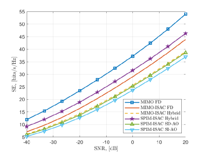
Figure 4: SE versus SNR when the radar-communications trade-off parameter $\varepsilon=0.5$.

V Numerical Experiments

We evaluated the performance of our SPIM-ISAC approach in comparison with FD and hybrid beamforming for MIMO-ISAC as well as SPIM-ISAC with SD-AO (Sec. IV-C3) and SI-AO beamformers [23], in terms of SE and beamforming gain averaged over $500$ Monte Carlo trials. The number of antennas at the BS and the users are $N_{\mathrm{T}}=128$ and $N_{\mathrm{R}}=16$, respectively. The carrier frequency and the bandwidth are selected as $f_{c}$ and $B=\frac{f_{c}}{10}$, respectively, and the number of subcarriers is $M=64$. We select the number of available spatial paths, unless stated otherwise, as $L=8$ ($L_{\mathrm{S}}=3$) and the number of targets is $K=2$. Thus, $P=10$, $N_{\mathrm{RF}}=5$ and $N_{\mathrm{S}}=3$. The target and path directions are drawn from $[-90^{\circ},90^{\circ}]$ uniformly at random, while the path gains are selected as $\gamma_{l}\sim\mathcal{N}(1,(0.1)^{2})$, $\forall l$ [15, 4].

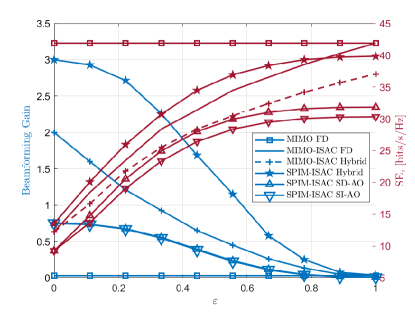
(a)

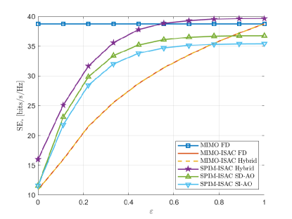
(b)

Figure 5: (a) SE and beamforming gain performance versus $\varepsilon$ when $(L,L_{\mathrm{S}})=(8,3)$. (b) SE versus $\varepsilon$ for $(L,L_{\mathrm{S}})=(12,10)$, when $\mathrm{SNR}=0$ dB.

Fig. 4 shows the SE with respect to SNR when the radar-communications trade-off parameter is $\varepsilon=0.5$. The computation of MIMO-ISAC and SPIM-ISAC are computed via (16) and (III-A), respectively. The MIMO FD beamformer ($\mathbf{F}_{\mathrm{opt}}[m]$) constitutes a benchmark while the JRC beamformer ($\mathbf{F}_{\mathrm{CR}}[m]$ in (42)) provides a trade-off between radar and communications. We observe from Fig. 4 that a significant improvement is achieved in SE with our proposed SPIM-ISAC hybrid beamforming approach compared to MIMO-ISAC even with JRC beamformer. Although hybrid beamformers are employed, the proposed SPIM approach provides higher SE thanks to additional transmitted information bits via SPIM. Note that similar observations have also been made in the literature [28] which, however, involves communications-only MIMO system design. When we compare the proposed SD- and SI-AO beamforming techniques, the former exhibits higher SE as compared to the latter as the former takes advantages of SD implementation. Thus, the SD-AO beamformer is resilient to beam-split with the cost of employing $(M-1)N_{\mathrm{T}}N_{\mathrm{RF}}$ phase shifters.

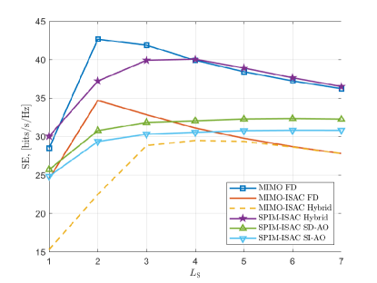
(a)

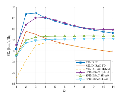
(b)

Figure 6: SE versus $L_{\mathrm{S}}$ for (a) $L=8$ and (b) $L=12$, respectively, when $\varepsilon=1$ and $\mathrm{SNR}=0$ dB.

Fig. 5 shows the system performance with respect to the trade-off parameter $\varepsilon$ for $(L,L_{\mathrm{S}})=(8,3)$. Specifically, Fig. 5(a) explicitly demonstrates the trade-off on both communications (SE) and radar (beamforming gain evaluated at target directions via (13)) metrics. We can see that as $\varepsilon\rightarrow 1$, SE of the competing algorithms increases whereas the beamforming gain decreases. Furthermore, the performance of the proposed SPIM approaches improves as $\varepsilon\rightarrow 1$, as expected, and they demonstrate even higher SE than the MIMO-ISAC JRC design, e.g, when approximately $\varepsilon>0.8$. In Fig. 5(b) the SE performance is presented for $(L,L_{\mathrm{S}})=(12,10)$. Compared to the case $(L,L_{\mathrm{S}})=(8,3)$ in Fig. 5(a), the results in Fig. 5(b) yields higher SE for all of the methods. Notably, the proposed SPIM-ISAC hybrid beamformer achieves much higher SE than that of MIMO FD beamformer for $\varepsilon\geq 0.6$ thanks to additional SE provided via SPIM with higher $L$ and $L_{\mathrm{S}}$. Fig. 5(b) also shows that SD- and SI-AO beamformers exhibit higher SE performance than that of MIMO-ISAC designs (hybrid and JRC) for up to $\varepsilon\geq 0.8$, however its performance falls behind the MIMO-ISAC beamformers as $\varepsilon$ further increases. This is because the AO beamformers have limited performance due to the absence of baseband beamformers.

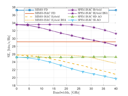
Figure 7: SE versus bandwidth for THz system with $f_{c}=300$ GHz when $\mathrm{SNR}=0$ dB and $\varepsilon=0.5$.

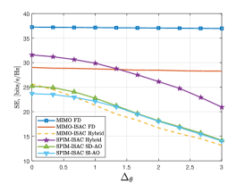
(a)

(b)

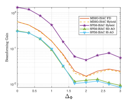
(c)

Figure 8: SE versus the mismatch on (a) DoD $\Delta_{\theta}$ and (b) DoA $\Delta_{\phi}$, and beamforming gain versus mismatch on (c) target DoAs $\Delta_{\Phi}$ when $\varepsilon=0.5$ and $\mathrm{SNR}=0$ dB.

Fig. 6 shows the SE performance with respect to number of selected SPIM paths $L_{\mathrm{S}}$ for (a) $L=8$ and (b) $L=12$, respectively, when $\varepsilon=0.5$ and $\mathrm{SNR}=0$ dB. As $L_{\mathrm{S}}$ increases, the performance of AO beamformers is saturated while the SE of the hybrid beamformers first increases then decreases. This is the result of sparse mmWave channel and the unoptimized power allocation of the baseband beamformers to less/more important path components, which can be compensated via multi-mode beamforming techniques [11]. When compared to the cases $L=8$ and $L=12$, higher SE is achieved for all algorithms in the latter. Furthermore, the proposed SPIM-ISAC hybrid beamformer achieves higher SE than that of MIMO FD beamformer for $L_{\mathrm{S}}\geq 4$ ($L_{\mathrm{S}}\geq 4$) when $L=8$ ($L=12$). Note that the performance improvement obtained from SPIM-ISAC is limited to the number of available spatial paths in the environment. Thus, one cannot always achieve higher SE by employing SM over more paths since the achieved SE is also limited by the number of RF chains at the cost of higher hardware complexity.

In order to demonstrate the performance of the proposed BSA hybrid beamforming technique, the SE of the beamformers are given in Fig. 7 with respect to the bandwidth $B\in[0,40]$ GHz. In this experiment, we consider the THz scenario with $f_{c}=300$ GHz. However, similar results can also be achieved if the same signal model is used for the mmWave scenario with $d=\frac{\lambda_{c}}{2}$, which corresponds to $f_{c}=\frac{300}{5}=60$ GHz and $B\in[0,8]$ GHz. We can see from Fig. 7 that the FD beamformers are not affected by the beam-split since they do not include analog components. The SD-AO beamformer also provides a robust performance against beam-split at the cost reduced SE since it is implemented in SD manner without baseband components. The proposed BSA approach is employed in MIMO-ISAC and SPIM-ISAC hybrid beamformers. We can see that the performance of proposed BSA approach yields robust performance up to approximately $B\leq 30$ GHz. Note that the performance of the proposed BSA hybrid beamforming approach is limited by the number of RF chains. In particular, the beam-split can be fully mitigated only if $\mathbf{F}_{\mathrm{RF}}^{(i)}{\mathbf{F}_{\mathrm{RF}}^{(i)}}^{\dagger}=\mathbf{I}_{\mathrm{N}_{\mathrm{T}}}$, which requires $N_{\mathrm{RF}}=N_{\mathrm{T}}$. Nevertheless, the proposed approach has satisfactory performance without employing additional hardware components, e.g., TD networks. In addition, the performance loss because of beam-split is further compensated thanks to additional SE gain via SPIM.

Fig 8 presents the performance analysis with respect to the angular mismatch in the estimated DoD and DoA angles (i.e., $\theta$ and $\phi$) of the communications user as well as the DoA angles of the radar targets (i.e., $\Phi$). During simulations, the mismatch DoD/DoA angles are generated as $\breve{\kappa}\sim\mathcal{N}(\kappa+\Delta_{\kappa},(0.1\Delta_{\kappa})^{2})$, where $\kappa\in\{\theta,\phi,\Phi\}$. Fig. 8(a) and Fig.8(b) show the SE with respect to $\Delta_{\theta}$ and $\Delta_{\phi}$, respectively, while Fig. 8(c) shows the beamforming gain with respect to $\Delta_{\Phi}$. We can see that the SE is more tolerable to the mismatch in $\phi$ than that of $\theta$ because of $N_{\mathrm{R}}<N_{\mathrm{T}}$.

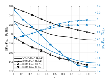
Figure 9: Beamforming error for JRC with respect to $\varepsilon$ when $(L,L_{\mathrm{S}})=(8,3)$ and $\mathrm{SNR}=0$ dB.

In order to present the system performance with respect to a joint metric for the beamformers, Fig. 9 shows the JRC performance in terms of the error between the hybrid beamformers and the communication/radar-only beamformers, i.e., $||\mathbf{F}_{\mathrm{RF}}\overline{\mathbf{F}}_{\mathrm{BB}}-\overline{\mathbf{F}}_{\mathrm{C}}||_{\mathcal{F}}$ and $||\mathbf{F}_{\mathrm{RF}}\overline{\mathbf{F}}_{\mathrm{BB}}-\mathbf{F}_{\mathrm{R}}\overline{\mathbf{\Pi}}||_{\mathcal{F}}$, respectively. we can see that the proposed SPIM-ISAC provides less error with respect to $\overline{\mathbf{F}}_{\mathrm{C}}$ and $\mathbf{F}_{\mathrm{R}}\overline{\boldsymbol{\Pi}}$ as compared to the competing beamformers.

Finally, we present the beampattern of the proposed SPIM-ISAC hybrid beamformer in Fig. 10 for $\eta=\{0,0.3,0.5,0.8,1\}$ when only $S=2$ ($i\in\{1,2\}$) spatial patterns are used. In this scenario, $K=1$ and $(L,L_{\mathrm{S}})=(2,1)$. The target is located at $\Phi_{1}=40^{\circ}$ while the BS receives the incoming paths from the communications user at $\theta_{1}=50^{\circ}$ ($i=2$) and $\theta_{2}=60^{\circ}$ ($i=2$), respectively. The beampattern becomes suppressed at the target direction when $\eta\rightarrow 1$. Conversely, the beampattern at the user locations is minimized when $\eta\rightarrow 0$. This illustrates the effectiveness of our proposed SPIM-ISAC approach.

Figure 10: Beampattern for $K=1$, $(L,L_{\mathrm{S}})=(2,1)$ when $(\Phi_{1},\theta_{1})$ is (top) $(40^{\circ},50^{\circ})$ ($i=1$) and (bottom) $(40^{\circ},60^{\circ})$ $(i=2)$, respectively, for various values of $\varepsilon=\{0,0.3,0.5,0.8,1\}$.

VI Summary

We introduced an SPIM framework for ISAC, wherein the hybrid beamformers are designed by exploiting the spatial scattering paths between the BS and the communications user. We have shown that a significant performance improvement is achieved via SPIM-ISAC compared to conventional MIMO-ISAC, wherein only the strongest path is selected for beamformer design. A family of beamforming techniques have been introduced including hybrid, BSA hybrid, SI-AO and SD-AO beamforming. The trade-off among these techniques has been investigated in terms of SE, beamforming gain and hardware complexity. Specifically, the SD-AO beamformer can accurately compensate the beam-split, however, it has high hardware complexity. Unlike SD-AO, SI-AO beamformer has simple architecture at the cost of lower SE. The proposed SPIM-ISAC hybrid beamformer takes advantage of employing baseband beamformer. The BSA hybrid beamforming technique achieves higher SE than the AO beamformers while having low hardware complexity. Furthermore, the proposed SPIM-ISAC hybrid beamforming approach exhibits significant spectral efficiency performance even higher than that of the usage of MIMO-ISAC FD beamformers in the presence of beam-split. As a result, the proposed SPIM-ISAC approach can be considered as a solution to the performance loss because of beam-split for both mmWave and THz systems.

Appendix A Proof of Lemma 1

The array gain varies across the whole bandwidth as

$$A_{G}({\Phi},{m})=\frac{|\mathbf{a}_{\mathrm{T}}^{\textsf{H}}(\Phi)\mathbf{a}_{\mathrm{T}}(\Phi_{m})|^{2}}{N_{\mathrm{T}}^{2}}.$$ (52)

By using (10), (52) is rewritten as

$$A_{G}({\Phi},{m}) =\frac{1}{N_{\mathrm{T}}^{2}}\left|\sum_{n_{1}=1}^{N_{\mathrm{T}}}\sum_{n_{2}=1}^{N_{\mathrm{T}}}e^{-\mathrm{j}\pi\left((n_{1}-1){\Phi_{m}}-(n_{2}-1)\frac{\lambda_{c}\Phi}{\lambda_{m}}\right)}\right|^{2}$$

$$=\frac{1}{N_{\mathrm{T}}^{2}}\left|\sum_{n=0}^{N_{\mathrm{T}}-1}e^{-\mathrm{j}2\pi nd\left(\frac{\Phi_{m}}{\lambda_{c}}-\frac{\Phi}{\lambda_{m}}\right)}\right|^{2}$$

$$=\frac{1}{N_{\mathrm{T}}^{2}}\left|\sum_{n=0}^{N_{\mathrm{T}}-1}e^{-\mathrm{j}2\pi nd\frac{(f_{c}\Phi_{m}-f_{m}\Phi)}{c_{0}}}\right|^{2}$$

$$=\frac{1}{N_{\mathrm{T}}^{2}}\left|\frac{1-e^{-\mathrm{j}2\pi N_{\mathrm{T}}d\frac{(f_{c}\Phi_{m}-f_{m}\Phi)}{c_{0}}}}{1-e^{-\mathrm{j}2\pi d\frac{(f_{c}\Phi_{m}-f_{m}\Phi)}{c_{0}}}}\right|^{2}$$

$$=\frac{1}{N_{\mathrm{T}}^{2}}\left|\frac{\sin(\pi N_{\mathrm{T}}\mu_{m})}{\sin(\pi\gamma_{m})}\right|^{2}=|\xi(\mu_{m})|^{2},$$ (53)

where $\mu_{m}=d\frac{(f_{c}\Phi_{m}-f_{m}\Phi)}{c_{0}}$. The array gain in (53) implies that most of the power is focused only on a small portion of the beamspace due to the power-focusing capability of $\xi(a)$, which substantially reduces across the subcarriers as $|f_{m}-f_{c}|$ increases. Furthermore, $|\xi(\mu_{m})|^{2}$ gives peak when $\mu_{m}=0$, i.e., $f_{c}\Phi_{m}-f_{m}\Phi=0$. Thus, we have $\Phi_{m}=\eta_{m}\Phi$, which completes the proof. ∎

References

• [1] K. V. Mishra, M. R. B. Shankar, V. Koivunen, B. Ottersten, and S. A. Vorobyov, “Toward millimeter-wave joint radar communications: A signal processing perspective,” IEEE Signal Process. Mag., vol. 36, no. 5, pp. 100–114, 2019.
• [2] A. M. Elbir, K. V. Mishra, S. Chatzinotas, and M. Bennis, “Terahertz-band integrated sensing and communications: Challenges and opportunities,” arXiv preprint arXiv:2208.01235, 2022.
• [3] F. Liu, C. Masouros, A. P. Petropulu, H. Griffiths, and L. Hanzo, “Joint radar and communication design: Applications, state-of-the-art, and the road ahead,” IEEE Trans. Commun., vol. 68, no. 6, pp. 3834–3862, 2020.
• [4] A. M. Elbir, K. V. Mishra, and S. Chatzinotas, “Terahertz-band joint ultra-massive MIMO radar-communications: Model-based and model-free hybrid beamforming,” IEEE J. Sel. Top. Signal Process., vol. 15, no. 6, pp. 1468–1483, 2021.
• [5] J. Liu, K. V. Mishra, and M. Saquib, “Co-designing statistical MIMO radar and in-band full-duplex multi-user MIMO communications,” arXiv preprint arXiv:2006.14774, 2020.
• [6] G. Duggal, S. Vishwakarma, K. V. Mishra, and S. S. Ram, “Doppler-resilient 802.11ad-based ultrashort range automotive joint radar-communications system,” IEEE Trans. Aerosp. Electron. Syst., vol. 56, no. 5, pp. 4035–4048, 2020.
• [7] S. Sedighi, K. V. Mishra, M. R. B. Shankar, and B. Ottersten, “Localization with one-bit passive radars in narrowband internet-of-things using multivariate polynomial optimization,” IEEE Trans. Signal Process., vol. 69, pp. 2525–2540, 2021.
• [8] V. Petrov, G. Fodor, J. Kokkoniemi, D. Moltchanov, J. Lehtomaki, S. Andreev, Y. Koucheryavy, M. Juntti, and M. Valkama, “On Unified Vehicular Communications and Radar Sensing in Millimeter-Wave and Low Terahertz Bands,” IEEE Wireless Commun., vol. 26, no. 3, pp. 146–153, 2019.
• [9] R. W. Heath, N. González-Prelcic, S. Rangan, W. Roh, and A. M. Sayeed, “An overview of signal processing techniques for millimeter wave MIMO systems,” IEEE J. Sel. Top. Signal Process., vol. 10, no. 3, pp. 436–453, 2016.
• [10] A. M. Elbir, K. V. Mishra, S. A. Vorobyov, and R. W. Heath Jr., “Twenty-five years of advances in beamforming: From convex and nonconvex optimization to learning techniques,” arXiv preprint arXiv:2211.02165, 2022.
• [11] A. Alkhateeb and R. W. Heath, “Frequency selective hybrid precoding for limited feedback millimeter wave systems,” IEEE Trans. Commun., vol. 64, no. 5, pp. 1801–1818, 2016.
• [12] A. M. Elbir, W. Shi, A. K. Papazafeiropoulos, P. Kourtessis, and S. Chatzinotas, “Terahertz-band channel and beam split estimation via array perturbation model,” arXiv preprint arXiv:2208.03683, 2022.
• [13] B. Wang, M. Jian, F. Gao, G. Y. Li, and H. Lin, “Beam squint and channel estimation for wideband mmWave massive MIMO-OFDM systems,” IEEE Trans. Signal Process., vol. 67, no. 23, pp. 5893–5908, 2019.
• [14] F. Gao, B. Wang, C. Xing, J. An, and G. Y. Li, “Wideband beamforming for hybrid massive MIMO terahertz communications,” IEEE J. Sel. Areas Commun., vol. 39, no. 6, pp. 1725–1740, 2021.
• [15] L. Dai, J. Tan, Z. Chen, and H. V. Poor, “Delay-phase precoding for wideband THz massive MIMO,” IEEE Trans. Wireless Commun., vol. 21, no. 9, pp. 7271–7286, 2022.
• [16] L. You, X. Qiang, C. G. Tsinos, F. Liu, W. Wang, X. Gao, and B. Ottersten, “Beam squint-aware integrated sensing and communications for hybrid massive MIMO LEO satellite systems,” IEEE J. Sel. Areas Commun., vol. 40, no. 10, pp. 2994–3009, 2022.
• [17] T. Mao, Q. Wang, Z. Wang, and S. Chen, “Novel index modulation techniques: A survey,” IEEE Commun. Surv. Tutorials, vol. 21, no. 1, pp. 315–348, 2018.
• [18] J. A. Hodge, K. V. Mishra, B. M. Sadler, and A. I. Zaghloul, “Reconfigurable intelligent surfaces for 6G wireless networks using index-modulated metasurface transceivers,” IEEE J. Sel. Topics Signal Process., 2023, in press.
• [19] J. A. Hodge, K. V. Mishra, and A. I. Zaghloul, “Intelligent time-varying metasurface transceiver for index modulation in 6G wireless networks,” IEEE Antennas Wirel. Propag. Lett., vol. 19, no. 11, pp. 1891–1895, 2020.
• [20] L. He, J. Wang, and J. Song, “Spatial modulation for more spatial multiplexing: RF-chain-limited generalized spatial modulation aided mm-wave MIMO with hybrid precoding,” IEEE Trans. Commun., vol. 66, no. 3, pp. 986–998, 2018.
• [21] J. A. Hodge, K. V. Mishra, and A. I. Zaghloul, “Reconfigurable metasurfaces for index modulation in 5G wireless communications,” in IEEE Int. Appl. Comput. Electromagn. Soc. Symp., 2019, pp. 1–2.
• [22] D. Ma, N. Shlezinger, T. Huang, Y. Shavit, M. Namer, Y. Liu, and Y. C. Eldar, “Spatial modulation for joint radar-communications systems: Design, analysis, and hardware prototype,” IEEE Trans. Veh. Technol., vol. 70, no. 3, pp. 2283–2298, 2021.
• [23] J. Wang, L. He, and J. Song, “Towards higher spectral efficiency: Spatial path index modulation improves millimeter-wave hybrid beamforming,” IEEE J. Sel. Top. Signal Process., vol. 13, no. 6, pp. 1348–1359, 2019.
• [24] Y. Ding, V. Fusco, A. Shitvov, Y. Xiao, and H. Li, “Beam index modulation wireless communication with analog beamforming,” IEEE Trans. Veh. Technol., vol. 67, no. 7, pp. 6340–6354, 2018.
• [25] S. Gao, X. Cheng, and L. Yang, “Spatial multiplexing with limited RF chains: Generalized beamspace modulation (GBM) for mmWave massive MIMO,” IEEE J. Sel. Areas Commun., vol. 37, no. 9, pp. 2029–2039, 2019.
• [26] L. He, J. Wang, and J. Song, “On generalized spatial modulation aided millimeter wave MIMO: Spectral efficiency analysis and hybrid precoder design,” IEEE Trans. Wireless Commun., vol. 16, no. 11, pp. 7658–7671, 2017.
• [27] X. Shi, J. Wang, C. Pan, and J. Song, “Low-complexity hybrid precoding algorithm based on log-det expansion for GenSM-aided MmWave MIMO system,” IEEE Trans. Veh. Technol., vol. 70, no. 2, pp. 1554–1564, 2021.
• [28] S. Guo, H. Zhang, P. Zhang, P. Zhao, L. Wang, and M.-S. Alouini, “Generalized beamspace modulation using multiplexing: A breakthrough in mmWave MIMO,” IEEE J. Sel. Areas Commun., vol. 37, no. 9, pp. 2014–2028, 2019.
• [29] F. Shu, X. Jiang, X. Liu, L. Xu, G. Xia, and J. Wang, “Precoding and transmit antenna subarray selection for secure hybrid spatial modulation,” IEEE Trans. Wireless Commun., vol. 20, no. 3, pp. 1903–1917, 2020.
• [30] P. Yang and X. Qiu, “Hybrid precoding aided secure generalized spatial modulation in millimeter wave MIMO systems,” IEEE Commun. Lett., vol. 25, no. 2, pp. 397–401, 2020.
• [31] G. Xia, Y. Lin, X. Zhou, W. Zhang, F. Shu, and J. Wang, “Hybrid precoding design for secure generalized spatial modulation with finite-alphabet inputs,” IEEE Trans. Commun., vol. 69, no. 4, pp. 2570–2584, 2020.
• [32] A. Raafat, M. Sefunç, A. Agustin, J. Vidal, E. A. Jorswieck, and Y. Corre, “Energy efficient transmit-receive hybrid spatial modulation for large-scale MIMO systems,” IEEE Trans. Commun., vol. 68, no. 3, pp. 1448–1463, 2019.
• [33] H. Chu, L. Zheng, and X. Wang, “Super-resolution mmWave channel estimation for generalized spatial modulation systems,” IEEE J. Sel. Top. Signal Process., vol. 13, no. 6, pp. 1336–1347, 2019.
• [34] O. Yurduseven, S. D. Assimonis, and M. Matthaiou, “Intelligent reflecting surfaces with spatial modulation: An electromagnetic perspective,” IEEE Open J. Commun. Soc., vol. 1, pp. 1256–1266, 2020.
• [35] T. Ma, Y. Xiao, X. Lei, P. Yang, X. Lei, and O. A. Dobre, “Large intelligent surface assisted wireless communications with spatial modulation and antenna selection,” IEEE J. Sel. Areas Commun., vol. 38, no. 11, pp. 2562–2574, 2020.
• [36] A. M. Elbir, S. Coleri, and K. V. Mishra, “Federated dropout learning for hybrid beamforming with spatial path index modulation in multi-user mmWave-MIMO systems,” in IEEE International Conference on Acoustics, Speech and Signal Processing, 2021, pp. 8213–8217.
• [37] Z. Xu, A. Petropulu, and S. Sun, “A joint design of MIMO-OFDM dual-function radar communication system using generalized spatial modulation,” in IEEE Radar Conference, 2020, pp. 1–6.
• [38] J. Zhang, “Clutter mitigation for joint RadCom systems based on spatial modulation,” arXiv preprint arXiv:2105.07328, 2021.
• [39] J. Zhang, “Beampattern and robust Doppler filter design for spatial modulation based joint RadCom systems,” arXiv preprint Arxiv:2105.08060, 2021.
• [40] S. Zhu, F. Xi, S. Chen, and A. Nehorai, “A low-complexity MIMO dual function radar communication system via one-bit sampling,” in IEEE International Conference on Acoustics, Speech and Signal Processing, 2021, pp. 8223–8227.
• [41] A. M. Elbir, K. V. Mishra, A. Çelik, and A. M. Eltawil, “Millimeter-wave radar beamforming with spatial path index modulation communications,” in IEEE Radar Conference, 2023, in press.
• [42] A. M. Elbir and S. Chatzinotas, “BSA-OMP: Beam-split-aware orthogonal matching pursuit for THz channel estimation,” IEEE Wireless Commun. Lett., p. 1, Feb. 2023.
• [43] H. Sarieddeen, M.-S. Alouini, and T. Y. Al-Naffouri, “An overview of signal processing techniques for terahertz communications,” Proc. IEEE, vol. 109, no. 10, pp. 1628–1665, 2021.
• [44] H. Yuan, N. Yang, K. Yang, C. Han, and J. An, “Hybrid beamforming for terahertz multi-carrier systems over frequency selective fading,” IEEE Trans. Commun., vol. 68, no. 10, pp. 6186–6199, 2020.
• [45] L. Yan, C. Han, and J. Yuan, “A Dynamic Array-of-Subarrays Architecture and Hybrid Precoding Algorithms for Terahertz Wireless Communications,” IEEE J. Sel. Areas Commun., vol. 38, no. 9, pp. 2041–2056, 2020.
• [46] X. Yu, G. Cui, J. Yang, L. Kong, and J. Li, “Wideband MIMO radar waveform design,” IEEE Trans. Signal Process., vol. 67, no. 13, pp. 3487–3501, 2019.
• [47] R. Schmidt, “Multiple emitter location and signal parameter estimation,” IEEE Trans. Antennas Propag., vol. 34, no. 3, pp. 276–280, 1986.
• [48] B. Friedlander and A. J. Weiss, “Direction finding for wide-band signals using an interpolated array,” IEEE Trans. Signal Process., vol. 41, no. 4, pp. 1618–1634, 1993.
• [49] F. Shu, Y. Qin, T. Liu, L. Gui, Y. Zhang, J. Li, and Z. Han, “Low-complexity and high-resolution DOA estimation for hybrid analog and digital massive MIMO receive array,” IEEE Trans. Commun., vol. 66, no. 6, pp. 2487–2501, 2018.
• [50] A. R. Chiriyath, B. Paul, G. M. Jacyna, and D. W. Bliss, “Inner bounds on performance of radar and communications co-existence,” IEEE Trans. Signal Process., vol. 64, no. 2, pp. 464–474, 2015.
• [51] S. H. Dokhanchi, B. S. Mysore, K. V. Mishra, and B. Ottersten, “A mmWave automotive joint radar-communications system,” IEEE Trans. Aerosp. Electron. Syst., vol. 55, no. 3, pp. 1241–1260, 2019.
• [52] J. R. Hurley and R. B. Cattell, “The procrustes program: Producing direct rotation to test a hypothesized factor structure,” Behav. Sci., vol. 7, no. 2, pp. 258–262, 1962.
• [53] J. Lee, T. Oh, J. Moon, C. Song, B. Lee, and I. Lee, “Hybrid beamforming with variable RF attenuator for multi-user mmWave systems,” IEEE Trans. Veh. Technol., vol. 69, no. 8, pp. 9131–9134, 2020.