Anomaly Detection in Aeronautics Data with Quantum-compatible Discrete Deep Generative Model

Abstract

Deep generative learning cannot only be used for generating new data with statistical characteristics derived from input data but also for anomaly detection, by separating nominal and anomalous instances based on their reconstruction quality. In this paper, we explore the performance of three unsupervised deep generative models—variational autoencoders (VAEs) with Gaussian, Bernoulli, and Boltzmann priors—in detecting anomalies in flight-operations data of commercial flights consisting of multivariate time series. We devised two VAE models with discrete latent variables (DVAEs), one with a factorized Bernoulli prior and one with a restricted Boltzmann machine (RBM) as prior, because of the demand for discrete-variable models in machine-learning applications and because the integration of quantum devices based on two-level quantum systems requires such models. The DVAE with RBM prior, using a relatively simple—and classically or quantum-mechanically enhanceable—sampling technique for the evolution of the RBM’s negative phase, performed better than the Bernoulli DVAE and on par with the Gaussian model, which has a continuous latent space. Our studies demonstrate the competitiveness of a discrete deep generative model with its Gaussian counterpart on anomaly-detection tasks. Moreover, the DVAE model with RBM prior can be easily integrated with quantum sampling by outsourcing its generative process to measurements of quantum states obtained from a quantum annealer or gate-model device.

Keywords Generative modeling  $\cdot$ Deep learning  $\cdot$ Variational autoencoder  $\cdot$ Anomaly detection  $\cdot$ Restricted Boltzmann machine  $\cdot$ Gibbs sampling  $\cdot$ Quantum-assisted machine learning

1 Introduction

The field of machine learning has experienced an explosion in the development of deep-learning methods at the beginning of the 21st century, due to the flexibility, scalability, and superior performance of deep learning in classification, prediction, data generation, anomaly detection, and other applications [Hinton et al., 2006, Bengio et al., 2006, LeCun et al., 2015, Goodfellow et al., 2016]. The phenomenal success of deep learning, which refers to machine-learning techniques that use artificial-neural-network models with many layers, has been enabled by the widespread availability of specialized graphics processing units (GPUs) to perform computing-intensive linear-algebra operations on vectors, matrices, and tensors. These algebraic structures hold the numerical values of the input, intermediate, and output layers of the (deep) network, as well as the values of the biases and weights that are applied to the hidden and output units (neurons) of the network. During network training, manipulations of vectors, matrices, and higher-order tensors are performed ubiquitously to compute the network’s output in the forward pass and the gradients to update the biases and weights in the backward pass [LeCun et al., 2015, Witten et al., 2017].

One way to characterize the training process of a neural network is to differentiate between supervised and unsupervised learning [Dayan and Abbott, 2005, Witten et al., 2017]. In supervised learning, a ‘teacher’ imposes a set of desired input-output relationships on the network. For example, the training set might contain an extra column that specifies the desired output of the network, such as a class label. The class label or other supervisory information is not available during testing, when the performance of the network is evaluated. In unsupervised learning, no such oversight is provided, and the network’s response is self-organized and solely relies on the interplay between external input, intrinsic connectivity, network dynamics, and the value of a cost function that the network attempts to minimize. Unsupervised learning is computationally more complex than supervised learning and still a largely unresolved problem in machine learning. It has attracted considerable research effort [Hinton et al., 1995, Bengio et al., 2006, Vincent et al., 2008] because it holds the potential to uncover the statistical structure and hidden correlations of large unlabeled datasets, which constitute the predominant form of today’s data.

Generative modeling is a machine-learning technique widely used in unsupervised learning. Generative modeling attempts to estimate the probability distribution of a dataset. To accomplish this goal, generative models frequently employ a set of latent variables that represent unobserved factors that influence the values of observed variables. Deep generative models such as generative adversarial networks [Goodfellow et al., 2020], variational autoencoders (VAEs) [Kingma and Welling, 2013], and deep belief networks [Hinton and Salakhutdinov, 2006] have been widely applied to machine-learning use cases in science and engineering. In the studies reported in this paper, we use VAEs for generative modeling because a VAE possesses an efficient inference mechanism, incorporates regularization via a prior, maximizes a lower bound on the log likelihood, and allows estimation of the log likelihood via importance sampling [Kingma and Welling, 2013, Burda et al., 2015]. VAEs employ the evidence lower bound (ELBO) as a variational lower bound on the exact log likelihood. The (negative) ELBO is a well-defined, fully differentiable, loss function whose gradients are used to efficiently optimize network weights through backpropagation, permitting competitive performance in mining large datasets.

The majority of VAE and other generative-model designs reported in the literature use continuous latent spaces because of the widespread applicability of the normal distribution, which is continuous, due to the central limit theorem and the difficulty of propagating gradients through discrete variables. However, many deep-learning use cases rely on discrete latent variables to represent the required distributions, such as in applications in supervised and unsupervised learning, attention models, language models, and reinforcement learning [Kingma et al., 2014, Jang et al., 2016, Maaløe et al., 2017]. In particular, if the values of latent variables are to be computed by quantum computers, the latent variables need to be discrete because projective qubit measurements in the computational basis produce eigenvalues of -1 or +1. See supplementary section S1 for a more in-depth account of the importance of discrete-variable models.

In previous studies, discrete VAEs (DVAEs) and quantum VAEs were used to generate new data from samples from the VAE’s latent space after the VAE had been trained on a dataset such as MNIST or Omniglot, and the quality of generation (fit of the VAE’s model distribution to the distribution of the input data) was assessed by estimating the log likelihood of test data [Rolfe, 2016, Vahdat et al., 2018a, b, Khoshaman et al., 2019, Khoshaman and Amin, 2018, Vinci et al., 2020, Vahdat et al., 2020]. In the studies reported in this paper, we use VAE models with continuous and discrete latent space to detect anomalies in aeronautics data. The datasets used comprise primarily 1-Hz recordings of operationally significant flight metrics from commercial flights. Subject matter experts analyzed the recorded data and identified operationally and safety-relevant anomalies during takeoff and approach to landing. The identification of flight-operations anomalies is important because they can foreshadow potentially serious aviation incidents or accidents.

The application of VAEs to anomaly-detection tasks has become increasingly popular in recent years. An and Cho [2015] suggested an anomaly-detection method in which the anomaly score of a VAE is used as a Monte Carlo estimate of the reconstruction log likelihood (called “reconstruction probability” in the paper). Xu et al. [2018] used a VAE for the detection of anomalies in univariate time series, preprocessed with sliding time windows, representing seasonal key performance indicators in web applications. Based on the success of deep recurrent neural networks (RNNs) in machine-learning applications with sequential data, several studies have incorporated RNNs in VAEs by equipping the VAE’s encoder and decoder with long short-term memory constructs [Chen et al., 2019, Wang et al., 2020, Zhang and Chen, 2019, Zhang et al., 2019, Park et al., 2018]. The LSTM-VAE approach was also applied to anomaly detection in telemetry data from the Soil Moisture Active Passive (SMAP) satellite and the Mars Curiosity rover [Su et al., 2019]. However, the training of a VAE equipped with an RNN architecture on multidimensional time series is computationally costly and may overlook local temporal dependencies. To remedy these shortcomings, Memarzadeh et al. [2020] designed a convolutional VAE (CVAE) and tested its performance in detecting anomalies in time series of various Yahoo! benchmark datasets and in time series spanning the takeoff phase of commercial flights, a task on which the model achieved state-of-the-art performance.

We developed convolutional VAEs with Gaussian, Bernoulli, and Boltzmann priors. The VAE with Gaussian prior has a continuous latent space, whereas the models with Bernoulli or Boltzmann prior have a discrete latent space. The Boltzmann prior is implemented as a restricted Boltzmann machine (RBM) [Smolensky, 1986], that is, as a network of stochastic binary units with full connectivity between visible and hidden units but no connectivity between visible units or between hidden units. The VAE with Gaussian prior and the RBM network of the VAE model with RBM prior are derivations of the CVAE model presented in Memarzadeh et al. [2020] and of the DVAE model depicted in Vinci et al. [2020], respectively. Overall, our studies aim to determine and compare the anomaly-detection performance of the Gaussian, Bernoulli, and RBM models. We want to find out if the anomaly-detection performance of a VAE with discrete latent space is competitive with that of a VAE with Gaussian prior and continuous latent variables, the standard choice of VAE type. Also, if a classical deep generative model with discrete latent variables exhibits a performance that is comparable or superior to that of a continuous-variable counterpart, it is worth exploring if a quantum-enhanced version of the discrete model can achieve a performance that exceeds that of the fully classical discrete model.

We report the results of three sets of experiments. Using a dataset with a drop-in-airspeed anomaly during takeoff, our baseline study explores the behavior of the VAE models during training, with an emphasis on the training behavior of the RBM model, and compares the models’ anomaly-detection performance when operating with either optimized or nonoptimal hyperparameters, as given by the performance metrics precision, recall, and F1 score. Our second study investigates the ability of our trained models to generalize (transfer) to a new dataset containing the same anomaly without re-tuning of hyperparameters and without or with post-training on the new dataset. Finally, we examine if the performance of the RBM model is robust to changes in anomaly type and phase of flight, by evaluating the model’s performance on a new dataset with delay-in-flap-deployment anomaly during approach to landing; for this study, the model’s hyperparameters were re-tuned and the model was re-trained on the dataset used.

The structure of the paper is as follows. In section 2, we review causal generative models, that is, probabilistic models that reconstruct input data from latent variables. The concept of variational inference, as an approximation to an intractable posterior distribution, and prior distributions used in generative modeling with continuous and discrete latent variables are described. Section 3 covers VAEs with continuous and discrete latent spaces. We describe the $\beta$-VAE, used in our experiments, a type of VAE model that allows a weighting of the autoencoding and Kullback-Leibler (KL)-divergence terms in the variational ELBO objective. Alternative formulations of RBM prior networks in the VAE’s latent space are also introduced. In section 4, we describe the methodology we used to evaluate our models’ anomaly-detection performance. In section 5, we present the experimental findings of our three studies, outlined in the preceding paragraph. We discuss model design and performance in section 6 and present our conclusions in section 7. The appendix and supplementary material contain additional information on concepts and experiments.

2 Causal generative modeling

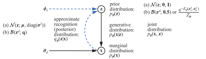
Figure 1: Generative models with latent variables, $\mathbf{z}$, can be represented as probabilistic graphical models that depict conditional relationships among variables. In a directed generative model, the model distribution, $p_{\bm{\theta}}(\mathbf{x},\mathbf{z})$ $=p_{\bm{\theta}}(\mathbf{x}|\mathbf{z})p_{\bm{\theta}}(\mathbf{z})$, is explicitly factored into the generative (decoder) distribution, $p_{\bm{\theta}}(\mathbf{x}|\mathbf{z})$, and the model’s prior distribution over latent variables, $p_{\bm{\theta}}(\mathbf{z})$. The marginal distribution, $p_{\bm{\theta}}(\mathbf{x})$, is obtained by marginalizing (integrating or summing) over the latent variables. Since the computation of the true posterior, $p_{\bm{\theta}}(\mathbf{z}|\mathbf{x})$, is intractable, variational inference substitutes it with an approximating posterior (encoder), $q_{\bm{\phi}}(\mathbf{z}|\mathbf{x})$. Black, solid arrows denote the generative model and blue, dashed arrows the variational approximation to the intractable posterior. In the VAE models used to conduct the experiments described in this paper, the posterior and prior over latent variables are either (a) continuous Gaussian distributions or (b) discrete Bernoulli or Boltzmann distributions. We use the symbolic expression $z^{d}$ to denote a discrete latent variable.

The goal of generative modeling is to estimate the probability distribution of the input data, $p(\mathbf{x})$, which is unknown but assumed to exist. The distribution of synthetic data points, estimated by the model, is called the marginal distribution, $p_{\bm{\theta}}(\mathbf{x})$ (where $\bm{\theta}$ denotes the model parameters). The goal is to make $p_{\bm{\theta}}(\mathbf{x})$ as close to $p(\mathbf{x})$ as possible. In order to accomplish this objective, representational modeling computationally analyzes the statistical structure of a dataset and attempts to identify a set of latent (unobserved) variables $\mathbf{z}$ that represent the dominant features of the dataset. Latent variables are also known as ‘causes’ [Dayan and Abbott, 2005]. A graphical model of a directed generative model with latent variables is depicted in figure 1. The generative model (decoder) reconstructs the input data from the latent variables [Dayan and Abbott, 2005, Kingma and Welling, 2019]. The statistics of the generative model’s output are given by the marginal distribution:

$$p_{\bm{\theta}}(\mathbf{x})=\int_{\mathbf{z}}p_{\bm{\theta}}(\mathbf{x},\mathbf{z})\mathrm{d}\mathbf{z}=\int_{\mathbf{z}}p_{\bm{\theta}}(\mathbf{x}|\mathbf{z})p_{\bm{\theta}}(\mathbf{z})\mathrm{d}\mathbf{z}.$$ (1)

Here, the joint distribution of the input variables $\mathbf{x}$ and the latent variables $\mathbf{z}$, $p_{\bm{\theta}}(\mathbf{x},\mathbf{z})$, defines the model distribution. In a directed generative model, the model distribution is explicitly factored into the generative distribution $p_{\bm{\theta}}(\mathbf{x}|\mathbf{z})$, the distribution of the generative model’s output given a latent-space realization, and the model’s prior distribution $p_{\bm{\theta}}(\mathbf{z})$. The marginal distribution is then obtained by integrating (‘marginalizing’) over the latent variables (see figure 1). If the latent variables are discrete, the integration in (1) is replaced by summation. Generative modeling is well suited for unsupervised learning: Lacking supervisory information, a model’s performance is determined by the ability of its latent variables to represent and reproduce the statistical structure of the input variables [Dayan and Abbott, 2005].

In representational learning, input-dependent latent variables (the ‘code’) are identified by a second model, the recognition model (encoder). The lower the number of latent variables is, the more compressed is the model’s latent space, with the degree of compression given by the ratio of input to latent variables. The statistical distribution of the recognition model’s output is called the recognition or posterior distribution, $p_{\bm{\theta}}(\mathbf{z}|\mathbf{x})$, the probability of the set of latent variables conditioned on the input data (see figure 1). The posterior distribution is given by Bayes’ rule as [Kingma and Welling, 2019]:

$$p_{\bm{\theta}}(\mathbf{z}|\mathbf{x})=\frac{p_{\bm{\theta}}(\mathbf{x},\mathbf{z})}{p_{\bm{\theta}}(\mathbf{x})}=\frac{p_{\bm{\theta}}(\mathbf{x}|\mathbf{z})p_{\bm{\theta}}(\mathbf{z})}{p_{\bm{\theta}}(\mathbf{x})}.$$ (2)

2.1 Variational inference

Models that allow the tractable computation of the posterior distribution are called invertible and those that do not noninvertible [Dayan and Abbott, 2005]. Noninvertible models do not allow gradient computations and concomitant optimization. Deep latent-variable models are noninvertible because no analytic solution or efficient estimation procedure exists for the marginal probability given in (1). Since the marginal is intractable, the posterior given in (2) is as well as it requires the marginal in its denominator [Kingma and Welling, 2019]. Approximate-inference techniques approximate the true posterior $p_{\bm{\theta}}(\mathbf{z}|\mathbf{x})$ and marginal $p_{\bm{\theta}}(\mathbf{x})$ [Dayan and Abbott, 2005, Kingma and Welling, 2019]. The approximate posterior is written as $q_{\bm{\phi}}(\mathbf{z}|\mathbf{x})$ (see figure 1). Variational inference is such an approximation technique. In variational inference, the marginal log likelihood is decomposed as follows [Kingma and Welling, 2013, 2019]:

$$\mathrm{log}\;p_{\bm{\theta}}(\mathbf{x})=D_{\mathrm{KL}}(q_{\bm{\phi}}(\mathbf{z}|\mathbf{x})||p_{\bm{\theta}}(\mathbf{z}|\mathbf{x}))+\mathcal{L}(\bm{\theta},\bm{\phi};\mathbf{x}).$$ (3)

The expression $D_{\mathrm{KL}}(p||q)\equiv\mathbb{E}_{p}\,\mathrm{log}[p/q]$ stands for the Kullback-Leibler (KL) divergence, an asymmetric ‘distance’ between two probability distributions. The term $\mathcal{L}(\bm{\theta},\bm{\phi};\mathbf{x})$ denotes the ELBO—a variational approximation, from below, to the true marginal log likelihood. As the KL divergence is non-negative, the ELBO is the greater and closer to the log likelihood, i.e., the bound tighter, the closer the approximating posterior is to the true posterior. Hence, maximizing the ELBO simultaneously increases the (log) likelihood and decreases the distance between the variational and true posteriors.

2.2 Prior distributions

The simplest generative-model priors are factorized standard normal or Bernoulli distributions:

$$\begin{split}p_{\bm{\theta}}(\mathbf{z})&=\mathcal{N}(\mathbf{z};\mathbf{0},\mathbf{I})\equiv\prod_{l=1}^{L}\mathcal{N}(z_{l};0,1),\cr p_{\bm{\theta}}(\mathbf{z}^{d})&=\mathcal{B}(\mathbf{z}^{d};\mathbf{0.5})\equiv\prod_{l=1}^{L}\mathcal{B}(z_{l}^{d};0.5),\end{split}$$ (4)

where the subscript $l$ denotes a latent variable. Also, we use the symbolic expression $z^{d}$ to denote a discrete latent variable (to delineate it from a continuous latent variable, expressed as $z$). The posterior distributions factorize accordingly [Khoshaman et al., 2019].

Boltzmann machine (BM) priors are more expressive and capable of representing complex multi-model probability distributions [Khoshaman et al., 2019]. Since Boltzmann priors are intractable in models with numbers of variables useful for practical problems, it is common to use Markov chain Monte Carlo (MCMC) sampling to estimate gradients. The efficiency of MCMC sampling is greatly increased [Khoshaman and Amin, 2018] by stipulating a bipartite connectivity between the groups of visible units $\mathbf{z}_{v}^{d}$ and hidden units $\mathbf{z}_{h}^{d}$ of the BM, without lateral connections between the units within either group, i.e., an RBM [Smolensky, 1986]. The visible and hidden units correspond to the input and latent variables, respectively, of an undirected generative model and are binary (0 or 1) in the RBMs we employed in the experiments reported in this paper. An RBM prior is given by [Welling et al., 2004, Salakhutdinov et al., 2007, Khoshaman et al., 2019]:

$$\begin{split}p_{\bm{\theta}}(\mathbf{z}_{v}^{d},\mathbf{z}_{h}^{d})&=\mathrm{e}^{-E_{\bm{\theta}}(\mathbf{z}_{v}^{d},\mathbf{z}_{h}^{d})}/Z_{\bm{\theta}},\quad Z_{\bm{\theta}}\equiv\sum_{\mathbf{z}_{v}^{d},\mathbf{z}_{h}^{d}}\mathrm{e}^{-E_{\bm{\theta}}(\mathbf{z}_{v}^{d},\mathbf{z}_{h}^{d})},\cr E_{\bm{\theta}}(\mathbf{z}_{v}^{d},\mathbf{z}_{h}^{d})&=-(\mathbf{z}_{v}^{d})^{\mathrm{T}}\mathbf{Wz}_{h}^{d}-\mathbf{a}^{\mathrm{T}}\mathbf{z}_{v}^{d}-\mathbf{b}^{\mathrm{T}}\mathbf{z}_{h}^{d}.\end{split}$$ (5)

In (5), $E_{\bf{\theta}}(\mathbf{z}_{v}^{d},\mathbf{z}_{h}^{d})$ is the energy function of visible and hidden units and $Z_{\bm{\theta}}$ the normalizing constant (partition function) of prior $p_{\bm{\theta}}(\mathbf{z}_{v}^{d},\mathbf{z}_{h}^{d})$; $\mathbf{W}$, $\mathbf{a}$, and $\mathbf{b}$ are the weight matrix between visible and hidden units and the visible and hidden bias vectors, respectively. The conditional distributions of the hidden given the visible units and of the visible given the hidden units are then given by [Witten et al., 2017]:

$$\begin{split}p_{\bm{\theta}}(\mathbf{z}_{h}^{d}|\mathbf{z}_{v}^{d})&=\prod_{l=1}^{L}p_{\bm{\theta}}((z_{h}^{d})_{l}|\mathbf{z}_{v}^{d})=\prod_{l=1}^{L}\sigma(b_{l}+\mathbf{W}_{\cdot l}^{\mathrm{T}}\,\mathbf{z}_{v}^{d}),\cr p_{\bm{\theta}}(\mathbf{z}_{v}^{d}|\mathbf{z}_{h}^{d})&=\prod_{k=1}^{K}p_{\bm{\theta}}((z_{v}^{d})_{k}|\mathbf{z}_{h}^{d})=\prod_{k=1}^{K}\sigma(a_{k}+\mathbf{W}_{k\cdot}\,\mathbf{z}_{h}^{d}),\end{split}$$ (6)

where $\sigma$ denotes the logistic function and $\mathbf{W}_{\cdot l}^{\mathrm{T}}$ is a vector consisting of the transpose of the lth column of weight matrix W and $\mathbf{W}_{k\cdot}$ a vector consisting of the kth row of W. Because of the absence of lateral connections between visible units and between hidden units, the conditional probabilities in (6) can be determined in one fell swoop, using block Gibbs sampling. In block Gibbs sampling, the values of all hidden units are updated at once by sampling from their conditional distribution given the visible units [top equation of (6)]. Then, the values of the visible units are updated analogously [bottom equation of (6)]. This process can be repeated for an arbitrary number of iterations. When Gibbs sampling is performed for an infinite number of steps, it is guaranteed to converge to the stationary distribution $p_{\bm{\theta}}(\mathbf{z}_{v}^{d},\mathbf{z}_{h}^{d})$ of the RBM model [Hinton, 2012, Fischer and Igel, 2014], and computationally efficient techniques to learn the model distribution have been developed [Hinton, 2002, Tieleman, 2008, Tieleman and Hinton, 2009].

3 Variational autoencoders

VAEs are directed generative models with latent variables that approximate the intractable true posterior $p_{\bm{\theta}}(\mathbf{z}|\mathbf{x})$ via variational inference and maximize an ELBO objective $\mathcal{L}(\bm{\theta},\bm{\phi};\mathbf{x})$ (see section 2.1 and figure 1). The ELBO can be re-written as [Kingma and Welling, 2013]:

$$\mathcal{L}(\bm{\theta},\bm{\phi};\mathbf{x})=\mathbb{E}_{\mathbf{z}\sim q_{\bm{\phi}}(\mathbf{z}|\mathbf{x})}[\mathrm{log}\;p_{\bm{\theta}}(\mathbf{x}|\mathbf{z})]-D_{\mathrm{KL}}(q_{\bm{\phi}}(\mathbf{z}|\mathbf{x})||p_{\bm{\theta}}(\mathbf{z})).$$ (7)

The first term of (7) is the autoencoding term. Maximizing it maximizes the fidelity of reconstruction because the greater the autoencoding term is, the greater is the similarity between the data distribution $p(\mathbf{x}$) and the generative distribution $p_{\bm{\theta}}(\mathbf{x}|\mathbf{z})$ when $\mathbf{z}$ is sampled from the approximate posterior distribution $q_{\bm{\phi}}(\mathbf{z}|\mathbf{x})$ of the encoder. Conversely, the second term is maximized by minimizing the KL divergence between the approximate posterior and prior, which corresponds to minimizing the mutual information between $\mathbf{x}$ and $\mathbf{z}$. Consequently, the autoencoding term attempts to maximize the mutual information between data and latents and the KL term seeks to minimize it. Eventually, the latent-space’s information content will depend on the trade-off between the two terms, which, in turn, is determined by the flexibility and expressiveness of the variational approximation $q_{\bm{\phi}}(\mathbf{z}|\mathbf{x})$, the structure of the generative model, and the training method [Khoshaman et al., 2019, Vinci et al., 2020].

Given training set $\mathcal{D}=\{\mathbf{x}^{(n)}\}_{n=1}^{N}$ consisting of N i.i.d. samples from $p(\mathbf{x})$, the ELBO for a minibatch of training data is given as the average of the ELBOs of the minibatch instances [Kingma and Welling, 2013]:

$$\mathcal{L}(\bm{\theta},\bm{\phi};\mathcal{M}^{(i)})=\frac{1}{M}\sum_{\mathbf{x}\in\mathcal{M}^{(i)}}\mathcal{L}(\bm{\theta},\bm{\phi};\mathbf{x}),$$ (8)

where the minibatch $\mathcal{M}^{(i)}=\{\mathbf{x}^{(i,m)}\}_{m=1}^{M}$ contains M data points randomly sampled from $\mathcal{D}$ with N data points.

3.1 VAE with factorized Gaussian prior

The ELBO objective given in (7) contains expectations of functions of the latent variables $\mathbf{z}$ with regard to the variational posterior $q_{\phi}(\mathbf{z}|\mathbf{x})$, which can be written as $\mathbb{E}_{\mathbf{z}\sim q_{\bm{\phi}}(\mathbf{z}|\mathbf{x})}[f(\mathbf{z})]$, where $f$ denotes an arbitrary function. To train the model with minibatch stochastic gradient descent starting from random initializations of the model parameters $\bm{\theta}$ and $\bm{\phi}$, we need to calculate gradients of such expectations [Kingma and Welling, 2019, Khoshaman et al., 2019]. Procedures to obtain unbiased gradients with respect to $\bm{\theta}$ and $\bm{\phi}$ are described in Appendix A.

We estimated the Gaussian parameters $\bm{\mu}$ and $\mathrm{log}\;\bm{\sigma}^{2}$ by means of linear layers at the top of the VAE’s encoder (see Appendix D). The $\mathrm{log}\;\bm{\sigma}^{2}$ estimate was then routed through a softplus activation. Hence, the mean and log variance of the approximate posterior, $\bm{\mu}$ and $\mathrm{log}\;\bm{\sigma}^{2}$, are nonlinear functions of the input data x and the variational parameters $\bm{\phi}$ [Kingma and Welling, 2013].

Moreover, when the VAE prior is given by a factorized Gaussian, the KL-divergence term in the ELBO objective [(7)] can be expressed in closed form. The ELBO is then estimated as:

$$\mathcal{L}(\bm{\theta},\bm{\phi};\mathbf{x})\simeq\frac{1}{S}\sum_{s=1}^{S}\mathrm{log}\;p_{\bm{\theta}}(\mathbf{x}|\mathbf{z}^{(s)})+\frac{1}{2}\sum_{l=1}^{L}(1+\mathrm{log}\>\sigma_{l}^{2}-\mu_{l}^{2}-\sigma_{l}^{2}),$$ (9)

where $\mathbf{z}^{(s)}=\bm{\mu}+\bm{\sigma}\odot\bm{\epsilon}^{(s)}$, $\bm{\epsilon}^{(s)}\sim\mathcal{N}(\mathbf{0},\mathbf{I})$, and $l$ indexes a latent variable [Kingma and Welling, 2013].

3.2 $\bm{\beta}$-VAE

Higgins et al. [2017] modified the VAE objective to reduce the entanglement between latent variables. Each latent variable $z_{l}$ is to represent a meaningful domain-specific attribute that varies along a continuum when $z_{l}$ is varied. In order to promote this disentangling property in the latent variables $\mathbf{z}\sim q_{\bm{\phi}}(\mathbf{z}|\mathbf{x})$, the authors introduce a constraint over the posterior $q_{\bm{\phi}}(\mathbf{z}|\mathbf{x})$ from which they are derived, making it more similar to a prior $p_{\bm{\theta}}(\mathbf{z})$, and thus restrain latent-space capacity and stimulate statistical independence between individual latent-space variables. The ELBO objective [(7)] of a $\beta$-VAE is given as (see Appendix B for derivation):

$$\mathcal{L}(\bm{\theta},\bm{\phi};\mathbf{x},\beta)=\mathbb{E}_{\mathbf{z}\sim q_{\bm{\phi}}(\mathbf{z}|\mathbf{x})}[\mathrm{log}\;p_{\bm{\theta}}(\mathbf{x}|\mathbf{z})]-\beta\,D_{\mathrm{KL}}(q_{\bm{\phi}}(\mathbf{z}|\mathbf{x})||p_{\bm{\theta}}(\mathbf{z})).$$ (10)

The parameter $\beta$ is used to balance the trade-off between the fit of the reconstructed data, $\hat{\mathbf{x}}$, to the input data, $\mathbf{x}$, imposed by the autoencoding (reconstruction) term (low $\beta$), and the fit of the posterior, $q_{\bm{\phi}}(\mathbf{z}|\mathbf{x})$, to the prior, $p_{\bm{\theta}}(\mathbf{z})$, via the KL term (high $\beta$). If $\beta=0$, the $\beta$-VAE model is identical to an autoencoder, and if $\beta=1$, the model corresponds to a regular VAE. We would like to note that we do not use $\beta$ to explicitly disentangle the latent space but employ it as a regularization hyperparameter that requires tuning, an approach pioneered in Memarzadeh et al. [2020].

3.3 VAE with discrete latent space

Several approaches have been developed to circumvent the non-differentiability problem affecting models with discrete latent units [Mnih and Gregor, 2014, Paisley et al., 2012, Gu et al., 2015, Bengio et al., 2013]. In VAE models, the reparameterization trick has been extended by either the incorporation of smoothing functions [Rolfe, 2016] or the relaxation of discrete latent variables into continuous ones [Jang et al., 2016, Maddison et al., 2016, Khoshaman and Amin, 2018]. In this work, we employ the Gumbel-softmax trick, which relaxes a discrete categorical distribution into a continuous concrete (or Gumbel-softmax) distribution [Maddison et al., 2016, Jang et al., 2016].

If each individual latent variable is sampled as $z^{d}\sim\mathcal{B}(p)$, where $\mathcal{B}$ denotes the Bernoulli distribution and $p$ its parameter, the concrete relaxation can be expressed as [Maddison et al., 2016]:

$$\mathbf{z}=\sigma((\mathrm{log}\;\bm{\alpha}+\mathrm{log}\;\bm{\rho}-\mathrm{log}(1-\bm{\rho}))/\lambda),$$ (11)

where $\sigma$ denotes the logistic function, $\sigma(x)=1/(1+e^{-x})$, $\alpha$ the odds of the Bernoulli probability, $\alpha=p/(1-p)$, $\rho$ a continuous uniform random variable on the interval [0, 1], and $\lambda$ the temperature of the concrete distribution. The temperature parameter $\lambda$ controls the degree of continuous relaxation: the greater $\lambda$ is, the greater is the relaxation and departure from a Bernoulli random variable, whereas small $\lambda$ values produce continuous variates close to 0 and 1. In our studies, we consistently use a $\lambda$ of 0.1, which we determined as a hyperparameter with good performance and which introduces only a small bias. The Gumbel-softmax relaxation was only applied during training and not during evaluation (validation or testing) because differentiability of the objective function is only required during the training phase and we sought to retain, where possible, the discrete character of the model and avoid the (slight) estimation bias introduced by the continuous relaxation. We estimated the log odds of the approximate relaxed Bernoulli posterior probabilities, $\mathrm{log}\;\bm{\alpha}^{\mathbf{q}}$, by means of a linear layer at the top of the VAE’s encoder (see Appendix D).

Discrete VAEs can be implemented with Bernoulli [bottom equation in (4)] or RBM [(5)] priors. Based on the probability mass function of a Bernoulli random variable, $\mathcal{B}(k;p)=p^{k}\;(1-p)^{1-k}$, the KL term of the ELBO of a VAE with a Bernoulli prior can be expressed as:

$$\begin{split}&D_{\mathrm{KL}}(q_{\bm{\phi}}(\mathbf{z}^{d}|\mathbf{x})||p_{\bm{\theta}}(\mathbf{z}^{d}))=\mathbb{E}_{\mathbf{z}^{d}\sim q_{\bm{\phi}}(\mathbf{z}^{d}|\mathbf{x})}[\mathrm{log}\frac{q_{\bm{\phi}}(\mathbf{z}^{d}|\mathbf{x})}{p_{\bm{\theta}}(\mathbf{z}^{d})}]\cr&=\mathbb{E}_{\mathbf{z}^{d}\sim\mathcal{B}(\mathbf{q})}[\sum_{l=1}^{L}\mathrm{log}\frac{q_{l}^{z_{l}^{d}}(1-q_{l})^{1-z_{l}^{d}}}{0.5^{z_{l}^{d}}(1-0.5)^{1-z_{l}^{d}}}]\cr&=\mathbb{E}_{\mathbf{z}^{d}\sim\mathcal{B}(\mathbf{q})}[\sum_{l=1}^{L}(z_{l}^{d}\;\mathrm{log}\;q_{l}+(1-z_{l}^{d})\,\mathrm{log}(1-q_{l})-z_{l}^{d}\;\mathrm{log}\;0.5-(1-z_{l}^{d})\,\mathrm{log}(1-0.5))]\cr&=\mathbb{E}_{\mathbf{z}^{d}\sim\mathcal{B}(\mathbf{q})}[\sum_{l=1}^{L}(-z_{l}^{d}\;\mathrm{log}\frac{0.5}{q_{l}}-(1-z_{l}^{d})\,\mathrm{log}\frac{1-0.5}{1-q_{l}})],\end{split}$$ (12)

where $q_{l}$ stands for the parameter of the latent Bernoulli variable $z_{l}^{d}\sim\mathcal{B}(q_{l})$, considered to be discrete, and 0.5 is the parameter of the Bernoulli prior distribution, $\mathcal{B}(p=0.5)$. The KL term can be implemented using the BCEWithLogitsLoss($\cdot$) function of the PyTorch nn module with the log-odds parameter vector of the respective relaxed Bernoulli distribution [$\mathrm{log}\;\bm{\alpha}^{\mathbf{q}}$ (approximate posterior) or $\mathrm{log}\;\bm{\alpha}^{\mathbf{p}}=\mathbf{0}$ (prior)] and the relaxed latent vector z (training) or hard latent vector $\mathbf{z}^{d}$ (evaluation) as input arguments. We used this (stochastic) method [Monte Carlo estimator of (12)] in all experiments in which the VAE had a Bernoulli prior. An analytic expression for the KL term in the ELBO objective [(7)] of a VAE with Bernoulli prior is given in Appendix C.

Since the applied concrete (Gumbel-softmax) relaxation replaces discrete latent variables $\mathbf{z}^{d}$ with continuous variables z, the KL term of the ELBO of a VAE with a relaxed Bernoulli posterior and an RBM prior can be expressed as:

$$\begin{split}&D_{\mathrm{KL}}(q_{\bm{\phi}}(\mathbf{z}|\mathbf{x})||p_{\bm{\theta}}(\mathbf{z}))\cr&=\mathbb{E}_{\mathbf{z}\sim q_{\bm{\phi}}(\mathbf{z}|\mathbf{x})}[\mathrm{log}\frac{q_{\bm{\phi}}(\mathbf{z}|\mathbf{x})}{p_{\bm{\theta}}(\mathbf{z})}]\cr&=\mathbb{E}_{\mathbf{z}\sim q_{\bm{\phi}}(\mathbf{z}|\mathbf{x})}[\mathrm{log}\;q_{\bm{\phi}}(\mathbf{z}|\mathbf{x})]-\mathbb{E}_{\mathbf{z}\sim q_{\bm{\phi}}(\mathbf{z}|\mathbf{x})}[\mathrm{log}\;p_{\bm{\theta}}(\mathbf{z})]\cr&=\mathbb{E}_{\mathbf{z}\sim q_{\bm{\phi}}(\mathbf{z}|\mathbf{x})}[\mathrm{log}\;q_{\bm{\phi}}(\mathbf{z}|\mathbf{x})]-\mathbb{E}_{\mathbf{z}\sim q_{\bm{\phi}}(\mathbf{z}|\mathbf{x})}[\mathrm{log}\frac{\mathrm{e}^{-E_{\bm{\theta}}(\mathbf{z})}}{Z_{\bm{\theta}}}]\cr&=\mathbb{E}_{\bm{\rho}\sim U(0,1)}[\mathrm{log}\;q_{\bm{\phi}}(\mathbf{z(\bm{\phi},\bm{\rho}})|\mathbf{x})]-\mathbb{E}_{\bm{\rho}\sim U(0,1)}[\mathrm{log}\frac{\mathrm{e}^{-E_{\bm{\theta}}(\mathbf{z(\bm{\phi},\bm{\rho}}))}}{Z_{\bm{\theta}}}]\cr&=\mathbb{E}_{\bm{\rho}\sim U(0,1)}[\mathrm{log}\;q_{\bm{\phi}}(\mathbf{z(\bm{\phi},\bm{\rho}})|\mathbf{x})]-\mathbb{E}_{\bm{\rho}\sim U(0,1)}[\mathrm{log}\;\mathrm{e}^{-E_{\bm{\theta}}(\mathbf{z(\bm{\phi},\bm{\rho}}))}]+\mathrm{log}\>Z_{\bm{\theta}}\cr&=\mathbb{E}_{\bm{\rho}\sim U(0,1)}[\mathrm{log}\;q_{\bm{\phi}}(\mathbf{z(\bm{\phi},\bm{\rho}})|\mathbf{x})]+\mathbb{E}_{\bm{\rho}\sim U(0,1)}[E_{\bm{\theta}}(\mathbf{z(\bm{\phi},\bm{\rho}}))]+\mathrm{log}\>Z_{\bm{\theta}}.\end{split}$$ (13)

Since $\nabla_{\bm{\theta}}\,\mathrm{log}\>Z_{\bm{\theta}}=-\nabla_{\bm{\theta}}\,\mathbb{E}_{\mathbf{\tilde{z}}^{d}\sim p_{\mathbf{\theta}}(\mathbf{\tilde{z}}^{d})}[E_{\bm{\theta}}(\mathbf{\tilde{z}}^{d})]$ [Khoshaman and Amin, 2018, Song and Kingma, 2021], unbiased gradients of the KL term with regard to the generative and variational parameters can be obtained as:

$$\nabla_{\bm{\theta},\bm{\phi}}\{\mathbb{E}_{\bm{\rho}\sim U(0,1)}[\mathrm{log}\;q_{\bm{\phi}}(\mathbf{z(\bm{\phi},\bm{\rho}})|\mathbf{x})]+\mathbb{E}_{\bm{\rho}\sim U(0,1)}[E_{\bm{\theta}}(\mathbf{z(\bm{\phi},\bm{\rho}}))]-\mathbb{E}_{\mathbf{\tilde{z}}^{d}\sim p_{\mathbf{\theta}}(\mathbf{\tilde{z}}^{d})}[E_{\bm{\theta}}(\mathbf{\tilde{z}}^{d})]\},$$ (14)

where the gradients of the log prior probability are given, as usual, as the difference between a positive and negative phase. The symbolic expression $\mathbf{\tilde{z}}^{d}$ denotes ‘fantasy states,’ i.e., values of the latent variables produced by the RBM model (prior) distribution, which remain discrete and are not relaxed during training [Khoshaman and Amin, 2018, Vinci et al., 2020]. In the expression above, we have highlighted the fact that the positive-phase energy [$E_{\bm{\theta}}(\mathbf{z(\bm{\phi},\bm{\rho}}))$] and the negative-phase energy [$E_{\bm{\theta}}(\mathbf{\tilde{z}}^{d})$] are calculated [according to the bottom equation of (5)] using relaxed posterior samples (z) and discrete model samples (fantasy states $\mathbf{\tilde{z}}^{d}$), respectively. The objective of training is to make the model distribution, $p_{\bm{\theta}}(\mathbf{\tilde{z}}^{d})$, as similar as possible to the posterior distribution, $q_{\bm{\phi}}(\mathbf{z}|\mathbf{x})$. We used the persistent-contrastive-divergence (PCD) algorithm [Tieleman, 2008] to evolve the conditional distributions of the ‘visible’ and ‘hidden’ layers of fantasy states of the negative phase by means of Gibbs sampling, starting from initialization to zero. In PCD, the chains of the fantasy states’ values are persistent and continue to evolve over cycles of training (minibatches), without re-initialization at the beginning of the cycle. The PCD algorithm is characterized by short mixing times (fast convergence to the stationary distribution) because the weight updates repel the persistent chains from their current states by raising the energies of the states [Hinton, 2012]. It should be noted that this form of training does not require knowledge of the (intractable) partition function $Z_{\bm{\theta}}$. Hence, our VAE model with RBM prior is an energy-based model whose training is based on (unnormalized) prior energies rather than (normalized) prior probabilities.

3.4 Latent Boltzmann networks

In a VAE with an RBM prior, the RBM network is located in the latent space; there are no visible RBM units corresponding to input data as in a standalone RBM. Also, by necessity, the latent variables $\mathbf{z}$ of the positive phase are continuous (because they are sampled from the approximate posterior distribution, which is relaxed via the Gumbel-softmax procedure described above during training in order to make the ELBO differentiable). On the other hand, the RBM model samples (fantasy states) $\mathbf{\tilde{z}}^{d}$ remain discrete variables, as indicated by the superscript, and are not relaxed during training.

Rolfe [2016] first developed a DVAE with RBM prior. The model applied the spike-and-exponential transformation to the posterior latents to make them differentiable. Khoshaman and Amin [2018] then modified the DVAE/RBM model by using the Gumbel-softmax trick to bring about the continuous relaxation of the DVAE’s latent variables; the authors termed their DVAE model with RBM prior and Gumbel-softmax relaxation ‘GumBolt.’ Vinci et al. [2020] introduced a quantum version of the GumBolt model, based on Amin et al. [2018] and Khoshaman et al. [2019]. These authors split up the posterior latent units $\mathbf{z}$ into two portions of equal size (denoted as $\mathbf{z}_{l}$ and $\mathbf{z}_{r}$ in figure 1) to implement between them the positive phase of the RBM model according to (14) and the energy function given in (5). A corresponding approach is taken for the fantasy states $\mathbf{\tilde{z}}^{d}$ of the negative phase. We designate an RBM model with such variables a ‘bipartite latent-space RBM.’ In such an RBM model, there is no difference in kind between the ‘visible’ and ‘hidden’ units (for example, $\mathbf{z}_{l}$ and $\mathbf{z}_{r}$, respectively, in the positive phase). The fantasy states are evolved via PCD Gibbs sampling whereas the posterior latent states remain ‘clamped’ to their original values (VAE encoder output) and are not subjected to Gibbs sampling.

Figure 1: Contrasting architectures of (a) a prior model in which an RBM is implemented between two subdivisions of the VAE’s latent space obtained by dividing the latent units $\mathbf{z}$ and $\mathbf{\tilde{z}}^{d}$, sampled from, respectively, the approximate posterior $q_{\bm{\phi}}(\mathbf{z}|\mathbf{x})$ and model prior $p_{\bm{\theta}}(\mathbf{\tilde{z}}^{d})$, into two equally sized parts each (here termed ‘bipartite latent-space RBM’) [Rolfe, 2016, Khoshaman and Amin, 2018, Khoshaman et al., 2019, Vinci et al., 2020] and of (b) a prior RBM model in which a true hidden layer is added to the layer of posterior latents, which constitute the ‘visible’ layer of the RBM’s positive phase (here termed ‘RBM with augmented positive phase’). Here, the symbolic expressions for the approximate posterior and prior distributions [$q_{\bm{\phi}}(\mathbf{z}|\mathbf{x})$ and $p_{\bm{\theta}}(\mathbf{\tilde{z}}^{d})$, respectively] highlight the fact that the posterior latents are relaxed into continuous random variables z whereas the prior latents (fantasy states) remain discrete variables $\mathbf{\tilde{z}}^{d}$. In a bipartite latent-space RBM, the latent states z of the approximate posterior remain ‘clamped’ to their original values (VAE encoder output) whereas the fantasy states $\mathbf{\tilde{z}}^{d}$ of the negative phase are evolved via PCD Gibbs sampling. In this work, we treat the latent variables $\mathbf{z}$ of the approximate posterior as the visible units of the RBM ($\mathbf{z}_{v}$) and add an equal number of hidden units ($\mathbf{z}_{h}^{d}$), thus augmenting the RBM’s positive phase. The values of $\mathbf{z}_{h}^{d}$ are determined by one-step Gibbs sampling, given the values of $\mathbf{z}_{v}$. The values of the ‘visible’ and ‘hidden’ units of the negative phase are evolved by PCD Gibbs sampling, as in the bipartite latent-space model. The symbol k denotes the number of Gibbs-sampling steps.

In the studies conducted for this paper, we have adopted a slightly different approach. We consider the posterior latent variables $\mathbf{z}$ to be inputs of the latent-space RBM ($\mathbf{z}_{v}$) and add an equal number of hidden units ($\mathbf{z}_{h}^{d}$) to the model. The values of the hidden units of the positive phase are determined by one-step Gibbs sampling, given the values of the visible units [see top equation of (6) for the hidden units’ distribution]. The values of the ‘visible’ and ‘hidden’ units of the negative phase ($\mathbf{\tilde{z}}_{v}^{d}$ and $\mathbf{\tilde{z}}_{h}^{d}$, respectively) are evolved by PCD Gibbs sampling, as in the bipartite latent-space model. We call a model with such features an ‘RBM with augmented positive phase.’ The contrasting architectures of the two models are shown in figure 1. We chose the model shown in figure 1(b) over the model in (a) to conduct our studies because it had displayed a more dynamic training and slightly better performance in preliminary experiments on the baseline dataset, using otherwise identical hyperparameters, including the number of VAE latents. When the model with augmented positive phase was used as the RBM prior, the mean latent values and mean energies of the positive and negative phases fluctuated more over minibatches of training before convergence to final values than when the bipartite latent-space RBM was used. Similarly, the components of the RBM bias vector b and the elements of the weight matrix W sometimes changed from decreasing to increasing or vice versa while converging to their final values over the epochs of training whereas the parameters of the bipartite latent-space RBM converged to their final values without much intermediary change of direction. The more lively training of the model depicted in figure 1(b) indicated to us that it might more easily switch between different modes of the system’s energy landscape than the faster or more directly converging model illustrated in (a). Lastly, the model in (b) produced slightly better performance metrics (precision, recall, and F1 score) in preliminary test runs on the baseline dataset. We would like to emphasize that we did not comprehensively evaluate and compare the training behavior and performance of the two models because such an assessment and comparison was not the focus of our studies. Both models performed similarly overall, as was to be expected considering their similar structures.

4 Evaluation of anomaly-detection performance

For the experiments reported in this paper, we trained 16 models (10 for the experiments assessing performance on the baseline dataset with nonoptimal hyperparameters; section 5.1.2) independently, and we report mean $+/-$ standard deviation. The reconstruction error of the ELBO [negative of left term in (9)] can be operationalized by the mean squared error (MSE) between the training data and the decoder output (reconstructed training data). We used this error metric when the input data were normalized by mean centering and scaling to unit variance (z score), which was the case for the datasets with drop-in-airspeed anomaly during takeoff. The MSE between the reconstructed and original training data is:

$$\mathrm{MSE}_{\mathbf{x}}=\frac{1}{S}\sum_{s=1}^{S}||\mathbf{x}^{(s)}-\hat{\mathbf{x}}^{(s)}||_{2}^{2},$$ (15)

where x symbolizes the input data and $\hat{\mathbf{x}}$ their reconstructions and the sum is taken over a minibatch of training data.

We used a different error metric to estimate the reconstruction error when the training data were normalized to lie between zero and one using the transformation

$$\mathbf{x}^{\prime}=\frac{\mathbf{x}-\mathrm{min}\{\mathbf{x}\}}{\mathrm{max}\{\mathbf{x}\}-\mathrm{min}\{\mathbf{x}\}},$$ (16)

where $\mathbf{x}^{\prime}$ symbolizes the transformed input data. This was the case for the dataset with a delay-in-flap-deployment anomaly during approach to landing. In this case, we used the binary cross entropy (BCE) to estimate the reconstruction error:

$$\mathrm{BCE}_{\mathbf{x}}=-\frac{1}{S}(\sum_{s=1}^{S}\sum_{j=1}^{J}x_{j}^{(s)}\;\mathrm{log}\;\hat{x}_{j}^{(s)}+(1-x_{j}^{(s)})\;\mathrm{log}(1-\hat{x}_{j}^{(s)})),$$ (17)

where the sums are over input instances and features. Our experiments showed that the BCE error metric captured the reconstruction error more accurately when the input data were scaled to the interval [0, 1].

Since nominal data points are much more prevalent than anomalous ones, the model primarily learns patterns exhibited by nominal data, and, therefore, their reconstruction errors (MSE or BCE) tend to be smaller than the errors of anomalous points. However, a powerful encoder-decoder model will also fit anomalous data points, which is undesirable when the reconstruction error is used as the metric to identify anomalies. To discourage the fitting to anomalous instances, our models are variational (rather than pure) autoencoders. The KL-divergence term in the ELBO of a VAE [(7)] penalizes the divergence between the approximate posterior $q_{\bm{\phi}}(\mathbf{z}|\mathbf{x})$ and prior $p_{\bm{\theta}}(\mathbf{z})$. We introduce the hyperparameter $\beta$ into the objective function [see (10)], based on the method developed in Higgins et al. [2017], to regulate the relative weighting of the autoencoding and KL terms of the ELBO. When $\beta$ is chosen properly, in such a way that the reduction in KL divergence due to the similarity between posterior and prior outweighs the rise in reconstruction error due to the lack of fit to (the few) anomalous data points, the model can be induced to preferentially fit data in the nominal majority class. Hence, optimal anomaly detection depends on careful tuning of the hyperparameter $\beta$.

Once a VAE model is trained with empirically optimized hyperparameters, we use the reconstruction errors per training instance, e, to determine an anomaly-score threshold. The threshold is based on the assumption that the data (nominal and anomalous instances) are normally distributed and is specified as:

$$thr=\langle e\rangle+z\Delta e,$$ (18)

where the angle brackets and $\Delta$ denote the mean and standard deviation, respectively, and z the z score, derived from the (known) percentage of anomalies in the training set using the quantile function. Once the threshold is determined based on the training data, we identify anomalies in the test data by calculating the anomaly score (reconstruction error) for each test data instance and comparing it to the above threshold; instances with an anomaly score below the threshold are classified as nominal, and instances with a score above the threshold are considered anomalous. Anomaly scores given by the BCE error metric are reasonably normally distributed. However, anomaly scores corresponding to the MSE metric are considerably skewed to the right and possess a long right tail. We applied various normalizing transformations to such anomaly scores, including the square-root, natural-logarithm, and inverse (reciprocal) transformation. On average, the logarithm produced the best anomaly-detection performance, and for this reason, we apply a log transformation to the anomaly scores from these datasets. We sampled both the threshold (based on the training set) and the (log-transformed) anomaly scores (based on the test set) ten times each and used the respective average values to classify data as nominal or anomalous. The thus predicted data labels, determined in an unsupervised way, are then compared with the known true data labels to compute performance metrics.

In all studies, we assume that the nominal data are the negative class and that the anomalous data are the positive class. We assess model performance with three metrics—precision, recall, and F1 score—specified as:

$$\begin{split}\mathrm{precision}&=\frac{TP}{TP+FP},\cr\mathrm{recall}&=\frac{TP}{TP+FN},\cr\mathrm{F1\;score}&=\frac{2}{\mathrm{recall}^{-1}+\mathrm{precision}^{-1}},\end{split}$$ (19)

where TP represents true positives: correctly identified anomalies, FP false positives (alarms): nominal instances incorrectly categorized as anomalous, and FN false negatives: missed anomalies or instances that were incorrectly classified as nominal.

5 Experimental results

All VAE models were implemented in Python using the PyTorch deep-learning library [Paszke et al., 2019]. Our VAE model with Gaussian prior is an upgraded version of the CVAE model introduced in Memarzadeh et al. [2020], which achieved state-of-the-art performance in detecting anomalies in aviation time series. In all models, the Adam optimizer was used, with a learning rate of $3\times 10^{-4}$ and default momentum parameters [Kingma and Ba, 2014]. We used minibatch-based optimization. Minibatches of mutually exclusive training-set instances were re-shuffled for each epoch of training. All minibatches comprised 128 training-set instances, except for the minibatches used for post-training in the transferability study (section 5.2), which contained 32 instances. We used validation sets to determine combinations of hyperparameter values with good performance. Except for the top layer of the encoder, which outputs the estimated parameters of the approximate posterior and the reparameterized latent variables (and effects the relaxation of discrete latent variables in discrete-variable models), all models use the same encoder and decoder architecture presented in Appendix D.

5.1 Baseline study: Drop in airspeed during takeoff

We determined the baseline performance of the VAE models with Gaussian, Bernoulli, and RBM priors on a dataset of departing flights with drop-in-airspeed anomaly. Subject matter experts ascertained that if the speed of an aircraft drops by more than 20 knots in the first 60 s after becoming airborne, an adverse event might ensue, and, therefore, data points with such a property are classified as anomalous. The dataset contains flight-operations data of commercial flights. It comprises primarily 1-Hz recordings for each flight that cover a variety of systems, including the state, orientation, and speed of the aircraft. The data are acquired in real time aboard the aircraft and downloaded by the airline once the aircraft has reached the destination gate. Each data instance is a 60 s-long recording of seven sensor outputs (five continuous, two discrete) during the initial ascent after becoming airborne. The drop-in-airspeed anomaly is not necessarily the only type of anomaly in the dataset, and the true number of operationally significant anomalies is unknown.

5.1.1 Model training

For this baseline study, we divided the data into training (60%), validation (20%), and test (20%) sets. We used the training set to train the models, the validation set to monitor overfitting and select hyperparameters, and the test set to assess model performance in an unbiased way. Since the input data were normalized by mean centering and scaling to unit variance, the MSE [(15)] was used to estimate the reconstruction error. Models were trained for 400 epochs. Model weights tended to converge at about 100 epochs. We did not observe any overfitting with increasing training time, as visualized by the change of the model’s loss [negative of the $\beta$-ELBO objective (10)] over time when evaluated on the validation set (figure 1 in the supplementary material).

We assessed many combinations of hyperparameters, separately for each model type (Gaussian, Bernoulli, RBM), and selected the hyperparameter values that produced the best overall performance in precision, recall, and F1 score. Our approach to use anomaly-detection performance on a validation set, assessed by comparing the data labels predicted by a model with the validation set’s known true labels, to tune model hyperparameters is comparable to the hyperparameter-optimization strategies employed in Memarzadeh et al. [2020] and Li et al. [2021]. The hyperparameters chosen for each model are given in table 1. The RBM model, which has a more flexible and expressive prior than the models with standard normal or Bernoulli prior, performed optimally at a lower latent-space dimensionality than the Gaussian and Bernoulli models. We also explored the application of a loss penalty to the RBM coupling weights W, the use of a sampling replay buffer, in which 5% randomly chosen fantasy states are not determined by the persistent chains but randomly set to 0 or 1 with equal probability [Du and Mordatch, 2019], KL-term annealing (‘warm-up’) [Sønderby et al., 2016], a hierarchical (conditional) posterior [Vahdat et al., 2020, Vinci et al., 2020], multiple sampling and averaging of the ELBO and its gradients [Vinci et al., 2020], and the continuous Bernoulli to normalize the ELBO’s reconstruction term [Loaiza-Ganem and Cunningham, 2019]. In the end, we did not apply any of these modifications because none of them improved the performance of our models, where applicable.

• Model prior	No. latentsa	betab	lambdac	No. fant. part.d	Len. pers. chainse
  Drop-in-airspeed anomaly during takeoff
  Gaussian	256	60	N/A	N/A	N/A
  Bernoulli	128	60	0.1	N/A	N/A
  RBM	64	60	0.1	500	20
  Delay-in-flap-deployment anomaly during approach to landing
  RBM	32	30	0.1	500	25

• ^a Number of latent units.

• ^b Hyperparameter $\beta$ controlling the balance between the autoencoding and KL terms.

• ^c Temperature of the relaxed Bernoulli distribution.

• ^d Number of fantasy particles / persistent chains.

• ^e Length of persistent chains.

Table 1: Hyperparameters used for the Gaussian, Bernoulli, and RBM models.

To assess model performance, the training and validation sets were combined, and the models were re-trained on the combined training/validation set. We then evaluated the performance of the models on the test set. The times of training the Gaussian, Bernoulli, and RBM models on the combined training/validation set for 400 epochs on a Skylake GPU-enhanced node of the Pleiades supercomputer at the NASA Ames Research Center are shown in table 2. The Gaussian and Bernoulli models as well as the RBM model with one PCD Gibbs-sampling update during the negative phase require about the same average training time [Gaussian: 1 h 0 min 29 s, Bernoulli: 58 min 27 s, RBM ($k=1$): 1 h 4 min 13 s]. On the other hand, the RBM model with 20 Gibbs updates requires, on average, more time to train [RBM ($k=20$): 1 h 34 min 17 s].

Table 2: Training times (400 epochs) of VAE models with
Gaussian, Bernoulli, and RBM priors when trained on the
combined training/validation set.

Model	Training time
Gaussian	1 h 00 min 29 s ($\pm$ 56 s)
Bernoulli	58 min 27 s ($\pm$ 19 s)
RBM ($k=1$)	1 h 04 min 13 s ($\pm$ 30 s)
RBM ($k=20$)	1 h 34 min 17 s ($\pm$ 19 s)

Times in parentheses indicate standard deviations.
The symbol $k$ stands for the number of Gibbs-sampling steps.

Figure 1 shows the values of the latent units of the positive phase [$\mathbf{z}\sim q_{\bm{\phi}}(\mathbf{z}|\mathbf{x})$] and of the negative phase [$\mathbf{\tilde{z}}^{d}\sim p_{\bm{\theta}}(\mathbf{\tilde{z}}^{d})$] averaged over latent dimensions and minibatch instances during a typical training run as well as the corresponding mean energies according to the bottom equation of (5), where visible and hidden units reside in the VAE’s latent space. Values for each minibatch (171 per epoch) are shown. The figure illustrates that the mean negative-phase values (of the latent variables and energy) closely follow their positive-phase counterparts. However, the mean negative-phase values fluctuate less and are more centered; these findings indicate that the (free-running) negative phase re-produces a smoothed and partially averaged version of the structure of the VAE latent units of the (clamped) positive phase.

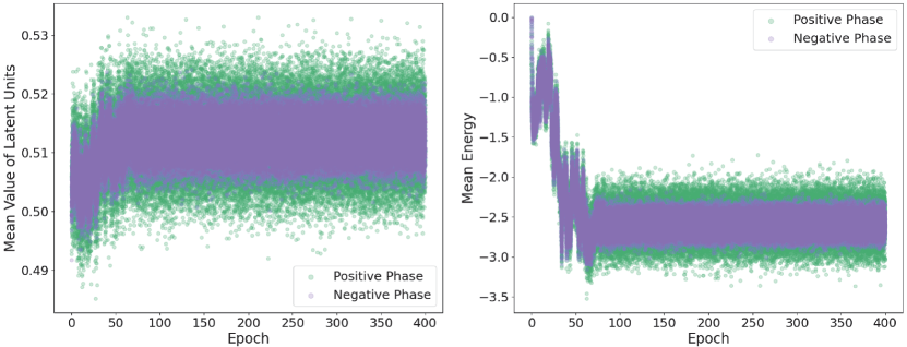
Figure 1: Values of latent units and energy, averaged over latent units and minibatch instances, of the positive phase [$\mathbf{z}\sim q_{\bm{\phi}}(\mathbf{z}|\mathbf{x})$] and of the negative phase [$\mathbf{\tilde{z}}^{d}\sim p_{\bm{\theta}}(\mathbf{\tilde{z}}^{d})$]. The average negative-phase values of these quantities are more centered than the corresponding average values of the positive phase, indicating that the negative phase re-produces a smoothed version of the posterior latents.

Training of the RBM biases and weights was dynamic, suggesting that the PCD algorithm explored well the energy landscape of the configurations of the system given by the dataset and model (figures 2 and 3 in the supplementary material). Histograms of log-transformed anomaly scores of the RBM model are shown in figure 1 for two training modes. We sampled both the anomaly-score threshold based on the training data as well as the test data’s anomaly scores ten times and used the sample statistics to gauge model performance, as described in section 4. We observed that models enter different modes during training and differ in their anomaly-detection performance depending on the selected mode. The mode with a threshold of about 5.7 for log-transformed anomaly scores produced the best model performance, with F1 scores $>$0.65. Training with modes with a threshold $\gtrsim$5.8, on the other hand, resulted in inferior model performance (F1 score $<$0.65). The superior performance of the mode with $thr\approx 5.7$ is illustrated by the cleaner separation of nominal and anomalous data. Modes with $thr\gtrsim 5.8$ , on the other hand, are characterized by a greater number of false positives (nominal data to the right of the anomaly-score threshold). Other modes, with thresholds between 5.7 and 5.8, were also observed but are less common.

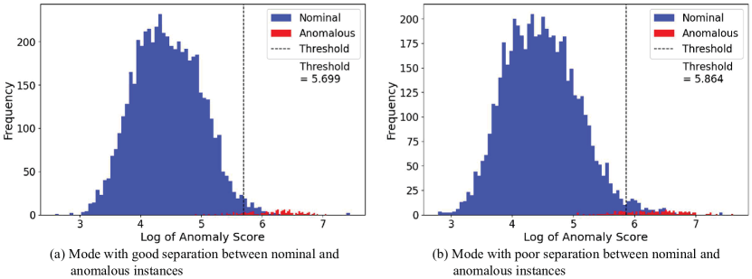
Figure 1: Histograms of average log-transformed anomaly scores for two training modes of the RBM model. Data points to the right of the dashed threshold line are categorized as anomalies. The mode with a threshold of $\sim$5.70 demonstrates a good separation of nominal and anomalous data, whereas the mode with a threshold of $\sim$5.86 exhibits a less good separation, with a relatively high number of nominal data classified as anomalies (false positives).

5.1.2 Model performance

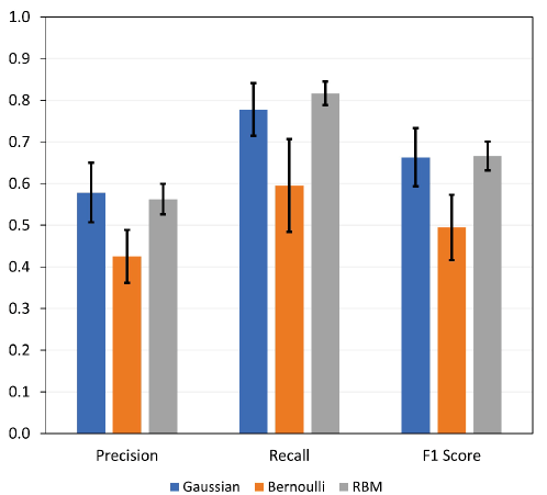
Figure 1: Performance of VAE models with Gaussian, Bernoulli, and RBM priors in the baseline study. Error bars indicate standard deviations of performance metrics among 16 independently trained models. Overall, the models demonstrate excellent performance on this unsupervised anomaly-detection task (average F1 score of 0.608). The more expressive discrete RBM model performs better than the simple discrete Bernoulli model and at a level comparable to the continuous Gaussian model. The DVAE appears to benefit from the flexibility and adaptability of the energy-based RBM prior.

The performance of the VAE models with Gaussian, Bernoulli, and RBM priors in the baseline study is shown in figure 1. The RBM model achieved a mean precision of 0.563, a mean recall of 0.817, and a mean F1 score of 0.666. The Gaussian model achieved a similar performance (pr 0.579, rc 0.778, f1 0.663). A notable observation is that the Bernoulli model lags behind both the RBM and the Gaussian model (pr 0.425, rc 0.596, f1 0.495). Our models demonstrate an excellent performance considering that the training was unsupervised and that the similar unsupervised CVAE model with Gaussian prior developed by Memarzadeh et al. [2020], which achieved state-of-the-art anomaly-detection performance on aviation datasets, achieved a precision of 0.31 and recall of 0.53 on a dataset similar to the one used in our baseline study. Both the Gaussian and Bernoulli models use the simplest factorized priors—the Gaussian model the continuous standard normal distribution and the Bernoulli model the discrete ‘standard’ Bernoulli distribution, with a parameter of 0.5. The models’ similar training times also attest to their comparability (see table 2). Comparing the two models with simple factorized priors, the continuous (Gaussian) model performs better on this dataset, which is dominated by continuous time-series inputs (5 continuous time series, 2 discrete/binary ones). On the other hand, the performance deficit of the simple Bernoulli model is offset by the more expressive RBM model, both of which are discrete VAE models. Precisely the RBM model’s flexibility and capability to adapt to the posterior distribution push it to a level of performance on par with the continuous Gaussian model. This observation highlights the performance boost accorded by energy-based modeling and MCMC sampling of the persistent states of the negative phase.

While training and evaluation with optimized hyperparameters allows a fair comparison between models, the approach leads to an overestimation of model performance when no validation set with labeled instances is available, as is frequently the case in practice, including in aeronautics applications. To give an impression of the performance of our models when nonoptimal hyperparameters are used, we trained models with all combinations between four different values for the latent-space dimensionality and five different settings for the hyperparameter $\beta$. The performance of models with 32, 64, 128, and 256 latent units as well as $\beta$ values of 1, 10, 25, 50, and 100 was evaluated. We trained ten Gaussian, Bernoulli, and RBM models each in this way for 300 epochs, which allowed model weights to converge to their final values, and averages of the resultant F1 scores are displayed as heatmaps in figure 1. The figure demonstrates the performance degradation that occurs when nonoptimal hyperparameters are used. A value of the hyperparameter $\beta$ of 50 or 100 is associated with moderate performance (F1 score between 0.314 and 0.536 across all three models), while a $\beta$ value of 1, 10, or 25 leads to poor performance (F1 score between 0.202 and 0.328). The influence of the hyperparameter $\beta$ on model performance is nonlinear, with a value of 1 or 25 resulting in better performance than a $\beta$ of 10. Performance differences due to different numbers of latent units are less pronounced. All latent-space dimensions investigated in this experiment (32, 64, 128, and 256) produce good performance and correspond to the latent-space dimensions employed in all studies described in this paper (see table 1).

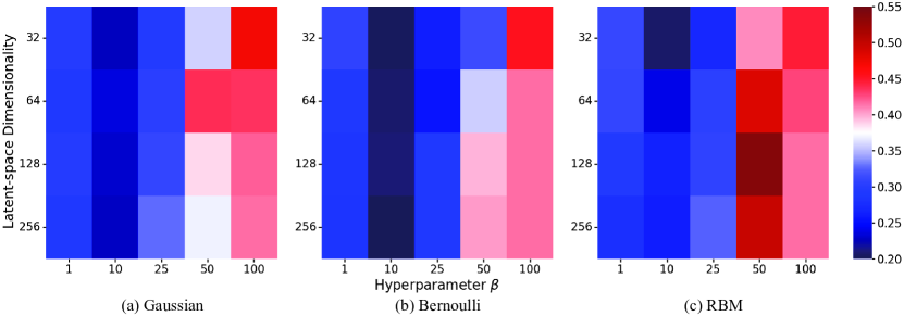
Figure 1: Performance of the Gaussian, Bernoulli, and RBM models in the baseline study after training with nonoptimal hyperparameters. The figure shows heatmaps of average F1 scores for the three models across the hyperparameters latent-space dimensionality and hyperparameter $\beta$, which are common to all three models. Across the three models, F1 scores are noticeably lower than after training with hyperparameters tuned based on validation-set performance, demonstrating the performance degradation incurred by using nonoptimal hyperparameters.

5.2 Model transferability

The DASHlink dataset used in this experiment consists of time series of sensor data collected during the first 60 s of the takeoff phase of commercial flights. This is a dataset collected independently of the dataset used in the baseline study (section 5.1) but containing the same input time series as the baseline dataset. The dataset also contains the same anomaly (drop in airspeed during takeoff by more than 20 knots) as the baseline dataset. The transferability study tests the ability of the models tuned and trained on the baseline data to transfer to another dataset containing the same input attributes and anomaly. All transferability experiments were conducted with hyperparameters determined by training on the baseline dataset’s training set and assessing model performance on the baseline dataset’s validation set (table 1). We examined two versions of transferability: a strong version of transferability, in which a model trained on the baseline data was directly tested on the DASHlink takeoff data, and a relaxed version, in which a model trained on the baseline data was post-trained on the DASHlink takeoff data for 300 epochs, with model weights initialized to the values acquired after training the model to convergence on the baseline data.

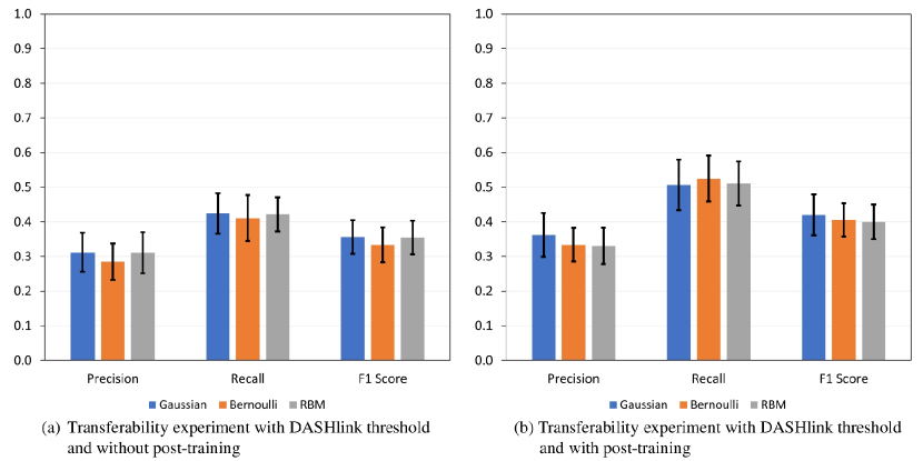
Figure 1: Performance of VAE models with Gaussian, Bernoulli, and RBM priors in the study examining the ability of the models tuned and trained on the baseline data to transfer to the DASHlink takeoff data. Error bars indicate standard deviations of performance metrics among 16 independently trained models. Performance was assessed based on a threshold derived from the DASHlink training set, (a) without or (b) with post-training on the new dataset for 300 epochs with model weights initialized by training to convergence on the baseline dataset. The figure depicts similar performance of all models, trained without supervision, markedly worse than in the baseline experiment, but still in the useful range.

The DASHlink takeoff dataset was split into training (50%) and test (50%) sets. The training set was used to determine the anomaly-score threshold [(18)] and the test set to compute log anomaly scores [log of (15)], which were used, in conjunction with the known data labels, to determine model performance. Results are shown in figure 1. The models with Gaussian, Bernoulli, and RBM priors performed similarly; all results are within each other’s error bounds (standard deviations of performance metrics among separately trained models). The average F1 scores of the Gaussian, Bernoulli, and RBM models are 0.356, 0.334, and 0.355, respectively, in the transferability experiment without post-training [figure 1(a)]. The values of this metric (in the same order) for the experiment with post-training are 0.420, 0.406, and 0.400 [figure 1(b)]. These results show that post-training on the target dataset slightly improves the overall F1-score average, by 6.03 percentage points. The relatively small extent of the performance improvement highlights the importance of hyperparameters for model performance. Comparing the baseline experiments and the transferability experiments with post-training, the model transfer reduced anomaly-detection performance (as measured by F1 score averaged across models) by 20.0 percentage points. The structure of the results is similar to that in the baseline study, with recall higher than precision. The Bernoulli model does not lag behind the other models, as in the baseline study. Overall, the model transfer markedly reduced model performance while still producing usable results. The transferability results are more difficult to interpret with regard to performance differences between the three models than the baseline results because the experiments from which they were obtained were more complex and involved additional factors (compared with the baseline experiments) since they involved two datasets. We report additional transferability experiments in supplementary section S2.

5.3 Robustness of RBM model: Delay in flap deployment during approach to landing

To deepen our insight into the behavior and performance of the VAE model with RBM prior, we conducted a further anomaly-detection study with this model, on another dataset, including de novo determination of hyperparameters and training. The experimental approach for this study is similar to the one adopted for the baseline study (section 5.1). The anomaly in the dataset used for this study is a delay in the deployment of flaps, as judged by a subject matter expert, during the final approach to landing, lasting approximately 160 s. As in the previous experiments, this labeled anomaly is not necessarily the only anomaly in the dataset, and the label is not among the model inputs during the unsupervised training. The dataset contains ten time series of aeronautical sensor outputs, relating to position, orientation, and speed of the aircraft, as well as to the positions of the control surfaces.

The dataset was divided into training (60%), validation (20%), and test (20%) sets. Since the data were normalized to lie in the range of zero to one using (16), we used the BCE [(17)] to estimate the reconstruction error [negative of left term in (9)]. Training proceeded for 400 epochs and weights converged to their final values after about 100 epochs. We again independently trained 16 models and report the mean +/- standard deviation of their performance. We did not observe any overfitting over the epochs of training, as visualized by the progression of the losses of the validation set. The hyperparameters tried out that produced the best overall performance in precision, recall, and F1 score, evaluated on the validation set, are given in table 1. To test model performance, the training and validation sets were combined for the purpose of model training, and then the performance of the models trained in this way was evaluated on the test set. It should be noted that in this study anomaly scores were not log-transformed because the original scores were already approximately normally distributed. Log transformation neither increased the scores’ normality nor improved anomaly-detection performance. Additional information is provided in supplementary section S3.

Table 3: Performance of the VAE model with RBM prior in the experiment
with late-deployment-of-flaps anomaly during final approach to landing.

Performance metric	Average	Standard deviation
Precision	0.591	0.0543
Recall	0.647	0.0564
F1 Score	0.618	0.0554

Table 3 shows the performance of the RBM model in this case study. The model achieved a mean precision of 0.591, a mean recall of 0.647, and a mean F1 score of 0.618. The mean F1 score is similar to (slightly lower than) the F1 value of 0.666 achieved by the RBM model in the baseline study, which was performed on a dataset with drop-in-airspeed anomaly during takeoff. Consequently, the late-deployment-of-flaps study corroborates the excellent anomaly-detection performance of the unsupervised VAE model with RBM prior observed in the baseline study and illustrates the model’s robustness to change of anomaly type and phase of flight.

6 Discussion

6.1 Model design

We developed two DVAE models. The Bernoulli model employs a factorized Bernoulli distribution as prior, in analogy to the common continuous VAE with Gaussian prior [(4)]. The RBM model is an attempt to make the DVAE more flexible and expressive. It places an RBM in the VAE’s latent space, so that the VAE’s latent units are the RBM’s inputs, and uses the energy-based restricted Boltzmann distribution given in (5) as prior. The RBM model parameters a, b, and W are tuned during training by the interplay between positive- and negative-phase energies, and the ‘visible’ and ‘hidden’ units of the negative phase (fantasy states $\mathbf{\tilde{z}}_{v}^{d}$ and $\mathbf{\tilde{z}}_{h}^{d}$, respectively) are updated via MCMC Gibbs sampling from (6).

DVAE models are less common than VAEs with continuous latent variables because an ELBO objective [(7)] containing discrete variables cannot be differentiated, thus precluding the computation of ELBO gradients, a necessary operation during the backward pass of training. In order to make DVAEs differentiable, the reparameterization trick [Kingma and Welling, 2013], which moves the variational parameters $\bm{\phi}$ from the distribution $q_{\phi}(\mathbf{z}|\mathbf{x})$ to a more easily differentiable deterministic function $g_{\bm{\phi}}(\bm{\epsilon},\mathbf{x})$, is extended by a smoothing function [Rolfe, 2016] or a continuous relaxation [Maddison et al., 2016, Jang et al., 2016]. Our Bernoulli and RBM models employ the Gumbel-softmax trick [Jang et al., 2016, Maddison et al., 2016] to relax the discrete posterior latents $\mathbf{z}^{d}\sim q_{\phi}(\mathbf{z}^{d}|\mathbf{x})$.

Several authors [Rolfe, 2016, Khoshaman and Amin, 2018, Khoshaman et al., 2019, Vinci et al., 2020] break up the VAE’s latent space into two equally sized partitions and implement the positive phase of the RBM between the two halves of latent units $\mathbf{z}$ sampled from the approximate posterior $q_{\bm{\phi}}(\mathbf{z}|\mathbf{x})$ and, similarly, the negative phase between the latent units $\mathbf{\tilde{z}}^{d}$ sampled from the RBM prior $p_{\bm{\theta}}(\tilde{\mathbf{z}}^{d})$. In this paper, we have termed an RBM model with such characteristics a ‘bipartite latent-space RBM.’ In the experiments performed for this paper, we have adopted a somewhat different approach and introduced a hidden layer in the RBM’s positive phase, which is obtained in one Gibbs-sampling step from the positive phase’s visible layer, comprising the VAE’s latent units. The evolution of the negative phase’s fantasy states is accomplished by Gibbs sampling in both RBM versions (see figure 1). We chose this augmented model rather than the bipartite latent-space one to conduct our experiments because it had demonstrated a somewhat more dynamic training and a slightly better performance in preliminary experiments that did not comprehensively evaluate the training behavior and performance characteristics of the two RBM model versions (see discussion at the end of section 3.3).

In addition to adding a truly hidden layer to the RBM’s positive phase, we also introduced the hyperparameter $\beta$ into the ELBO objective function [see (10)]. While Higgins et al. [2017] devised the $\beta$-ELBO, in which $\beta$ regulates the trade-off between the autoencoding and KL-divergence terms, as a way to promote disentanglement between latent dimensions by enforcing a minimum similarity between variational posterior $q_{\bm{\phi}}(\mathbf{z}|\mathbf{x})$ and prior $p_{\bm{\theta}}(\mathbf{z})$, we tune $\beta$ to optimize anomaly-detection performance, as measured by performance metrics [(19)].

6.2 Model performance

We assessed the performance of our VAE models with Gaussian, Bernoulli, and RBM priors in the context of anomaly detection in commercial aeronautics. Prior DVAE models used generation performance on MNIST [LeCun, 1998] and other image datasets to gauge model performance [Rolfe, 2016, Khoshaman and Amin, 2018, Khoshaman et al., 2019, Vinci et al., 2020]. Generation performance is quantified by the test-set log likelihood or a surrogate such as the ELBO or Q-ELBO. In our anomaly-detection studies, we used the performance metrics precision, recall, and F1 score. The accurate and timely discovery of flight-operations anomalies is important because they can be precursors of potentially serious aviation incidents or accidents. To detect operationally significant anomalies in flight data and preempt future accidents, airlines and transportation agencies will have to increasingly rely on advanced machine-learning techniques applied to historical data or online data streams. Multifactorial and nonlinear anomalies defy traditional anomaly-detection methods, such as exceedance detection [Federal Aviation Administration, 2004, Dillman et al., 2015], and the volume and proportion of anomalies characterized by heterogeneous and high-order feature interactions is only expected to increase with increasing airspace complexity, characterized by increasing passenger volume, the integration of unmanned aircraft systems, and urban air mobility. Since labeled data (i.e., data classified as either nominal or anomalous) are costly to obtain and frequently not available and many complex anomalies unknown, unsupervised learning approaches, such as the one portrayed in this paper, are often the preferred or only feasible option.

Both the Gaussian and the Bernoulli models employ simple factorized priors and require similar time to train (table 2). In these respects, the Bernoulli model is the discrete equivalent of the continuous Gaussian model. The anomaly-detection performance of the three models compares favorably with the performance of a recently developed CVAE and of other unsupervised machine-learning methods, evaluated on a related anomaly-detection task, described in Memarzadeh et al. [2020]. Our three models achieved F1 scores of $0.663\pm 0.0700$ (Gaussian), $0.495\pm 0.0785$ (Bernoulli), and $0.666\pm 0.0345$ (RBM) when tested on the baseline dataset with drop-in-airspeed anomaly during takeoff. Consequently, the Gaussian and RBM models perform at a similar level, whereas the Bernoulli model falls short in performance. In other words, the performance of the discrete model with simple factorized prior, which is inferior to the capability of the corresponding continuous model, is elevated to the performance of the continuous model by the adoption of a more flexible and expressive energy-based RBM prior that is able to more accurately represent the statistical structure of the input data. Hence, we have implemented an unsupervised discrete deep generative model that performs on par with the analogous continuous generative model that employs a Gaussian prior in detecting anomalies in an aeronautical dataset. The performance decrement due to the usage of nonoptimal hyperparameters was also assessed (figure 1). Our continuous and discrete models performed similarly in the transferability study (section 5.2). Our RBM model is ready to be integrated with quantum computing: the discrete (fantasy) states of the negative phase can be obtained by quantum Boltzmann sampling, by, for example, a quantum annealer or quantum-circuit Born machine (QCBM). On the other hand, a Gaussian VAE, the most common choice in classical deep generative learning, defies a straightforward integration with quantum sampling because it does not sample discrete states from a system whose generative process can be implemented by measuring a parameterizable density operator $\rho_{\bm{\theta}}$ or wave function $\psi_{\bm{\theta}}$ in the computational basis.

The proposed VAE model with RBM prior is robust to change of anomaly type and phase of flight, as demonstrated by its performance on a dataset with late-deployment-of-flaps anomaly during approach to landing, on which it achieved an F1 score of $0.618\pm 0.0554$ (section 5.3). Transfer to a novel dataset without renewed tuning of hyperparameters markedly decreases model performance. The RBM model’s F1 score on a dataset on which it was neither tuned nor trained but which contained the same input data and anomaly and spanned the same phase of flight was $0.355\pm 0.0486$, 31.1 percentage points lower than the performance on the dataset from which the transfer occurred. While such a drop represents a significant deterioration in performance, the post-transfer performance is still respectable, considering that the datasets involved consist of multiple complex time series and the training was executed without supervision. Transferability was mildly improved by post-training on the target dataset: initializing model weights to the (converged) values obtained at the end of training on the original dataset, post-training on the new dataset for 300 epochs raised the RBM model’s average F1 score by 4.51 percentage points to a value of 0.400.

Latent-space dimensionality and the hyperparameter $\beta$ are hyperparameters that have a strong effect on model performance (in all three models) and require optimization for each application. Models with 32–256 latent units generally exhibited good performance, whereas model performance was very sensitive to the specific choice of $\beta$; hence, the choice of the value of the hyperparameter $\beta$ is application-specific. The temperature $\lambda$ of the concrete distribution [Maddison et al., 2016, Jang et al., 2016], which determines the bias introduced by the continuous Gumbel-softmax relaxation and the differentiability of the model parameters, is also important for the discrete models (Bernoulli and RBM) and requires tuning. We used a $\lambda$ of 0.1 throughout our studies because it balances the trade-off between estimation bias and differentiability and had proved the optimal value among the ones tested. We did not use an annealing schedule to gradually reduce $\lambda$ over the epochs of training, but we used discrete (‘hard’) Bernoulli variables for validation and testing. While the length of the persistent chains (fantasy particles) had a mild influence on the performance of the RBM model, the number of fantasy particles was quite unimportant, due to the averaging of the particles’ (negative-phase) energies at the end of each series of Gibbs updates (per minibatch); we used 500 throughout. When optimal, or even adequate, hyperparameters are unknown and labeled data not available, which is often the case in practical applications, the performance of unsupervised anomaly-detection models can frequently be improved by making the effort to prepare a small labeled validation set that includes relevant anomalies and using it for hyperparameter tuning [Soenen et al., 2021, Antoniadis et al., 2022].

Mean negative-phase values of the latent variables and energy tightly followed the corresponding values of the positive phase, but were more centered, suggesting that the free-running negative phase re-produces a smoothed version of the clamped positive phase (figure 1). We were able to boost anomaly-detection performance by applying a normalizing transformation to skewed anomaly scores (MSEs) with conspicuous right tail. We always used a log transformation, but less skewed scores might benefit more from a square-root transformation and for more strongly skewed scores an inverse transformation might be optimal. We would like to note that our VAE models with continuous and discrete priors are universal generative models and not limited in application to aeronautics data, but, with slight modification, can also be applied to other time-series data.

7 Conclusions

We developed unsupervised VAE models with convolutional encoder and decoder layers and a latent space based on Gaussian, Bernoulli, and RBM priors. The discrete Bernoulli and RBM versions are an attempt to design models whose latent space captures the discrete nature of objects processed by machine-learning models, such as semantic classes, causal factors, digital samples, and other discrete entities. The RBM model allows a straightforward integration with quantum computing because the fantasy states of the RBM’s negative phase can be obtained by measuring the states of a quantum generative process, such as a quantum Boltzmann machine (QBM) implemented on an annealer or a QCBM on a circuit. Our objective is the maximization of the $\beta$-ELBO, in which the hyperparameter $\beta$ regulates the trade-off between reconstruction fidelity and regularization via a prior distribution placed on the latent variables.

We tested our VAE models on datasets comprising time series of commercial flights that contain anomalies during the takeoff or approach-to-landing phases of flight. It is expected that the use of unsupervised and semi-supervised machine-learning techniques to identify anomalies in aviation is going to increase because of the high cost of labeling instances manually, the limitations associated with the identification of anomalies based on simple heuristics, and the ever increasing airspace complexity over the course of the 21st century. While the estimated generative log likelihood or a related quantity is used to gauge generative-model performance in re-generation studies (e.g., of imagery), anomaly detection relies on metrics such as precision, recall, and F1 score to assess model performance.

While all unsupervised models exhibit good performance overall, the discrete Bernoulli model performs more poorly than the other two. However, the more expressive RBM model, which, during training, employs unnormalized energies rather than probabilities and MCMC to sample from the prior distribution, is a discrete-variable model whose performance matches that of the continuous Gaussian model. Our models are robust to changes in type of anomaly and phase of flight. Transferring a model without re-tuning of hyperparameters or re-training to a new dataset with the same anomaly results in an anomaly-detection performance that is markedly impaired, but still acceptable, considering the nature of the data and training.

In future studies, we will use more advanced algorithms, such as parallel tempering and adaptive-step PCD, to conduct negative-phase sampling, to see if such schemes improve model performance. We will also devise an estimator of the log partition function, to compute log-likelihood estimates for future generation studies. We also intend to use conditional VAEs or other deep generative models to generate artificial anomalies, to enhance anomaly-detection datasets and, ultimately, the performance of anomaly-detection algorithms. We plan to integrate quantum capabilities by developing a QBM, implemented by quantum annealing or QCBM. In addition, we intend to increase the expressiveness of our prior model by replacing the relatively simple RBM network with a more sophisticated energy-based feedforward network, and we will attempt to integrate such an EBM with quantum computing.

Appendix A. Unbiased gradients with respect to generative and variational parameters of VAE with factorized Gaussian prior

Unbiased gradients with respect to the generative parameters $\bm{\theta}$ are straightforward to obtain, and we can write:

$$\nabla_{\bm{\theta}}\mathbb{E}_{\mathbf{z}\sim q_{\bm{\phi}}(\mathbf{z}|\mathbf{x})}[f(\mathbf{z})]=\mathbb{E}_{\mathbf{z}\sim q_{\bm{\phi}}(\mathbf{z}|\mathbf{x})}[\nabla_{\bm{\theta}}f(\mathbf{z})]\simeq\frac{1}{S}\sum_{s=1}^{S}\nabla_{\bm{\theta}}f(\mathbf{z}^{(s)}).$$ (A1)

The mean on the right of (A1) is a Monte Carlo estimate of the gradient with respect to $\bm{\theta}$, in which $\mathbf{z}^{(s)}$ is an i.i.d. sample from $q_{\bm{\phi}}(\mathbf{z}|\mathbf{x})$ and $S$ indicates the size of the minibatch.

Unbiased gradients with respect to the variational parameters $\bm{\phi}$ are more difficult to obtain because the expectations in (7) are estimated by sampling from a probability distribution that depends on $\bm{\phi}$ [Khoshaman et al., 2019]. Based on the gradient of the logarithm of $q_{\bm{\phi}}$, $\nabla_{\bm{\phi}}\,\mathrm{log}\>q_{\bm{\phi}}$, the score-function estimator [Fu, 2006, Williams, 1992, Glynn, 1990] calculates gradients with respect to $\bm{\phi}$ as:

$$\nabla_{\bm{\phi}}\mathbb{E}_{\mathbf{z}\sim q_{\bm{\phi}}(\mathbf{z}|\mathbf{x})}[f(\mathbf{z})]=\mathbb{E}_{\mathbf{z}\sim q_{\bm{\phi}}(\mathbf{z}|\mathbf{x})}[f(\mathbf{z})\nabla_{\bm{\phi}}\mathrm{log}\>q_{\bm{\phi}}(\mathbf{z}|\mathbf{x})]\simeq\frac{1}{S}\sum_{s=1}^{S}f(\mathbf{z}^{(s)})\nabla_{\bm{\phi}}\mathrm{log}\>q_{\bm{\phi}}(\mathbf{z}^{(s)}|\mathbf{x})).$$ (A2)

Here, we assumed for simplicity that $f$ does not depend on $\bm{\phi}$. Unfortunately, gradients based on the score-function estimator are characterized by high variance and require the use of intricate variance-reduction techniques (such as control variates) in practical applications [Mnih and Gregor, 2014, Grathwohl et al., 2017].

The reparameterization trick [Kingma and Welling, 2013] is used in VAEs as a low-variance alternative to the score-function estimator. Here, the random variable $\mathbf{z}\sim q_{\bm{\phi}}(\mathbf{z}|\mathbf{x})$ is re-expressed by means of an auxiliary random variable $\bm{\epsilon}\sim p(\bm{\epsilon})$ independent of $\bm{\phi}$ and a deterministic function $g_{\bm{\phi}}(\cdot)$ as $\mathbf{z}=g_{\bm{\phi}}(\bm{\epsilon},\mathbf{x})$. We then can write $\mathbb{E}_{\mathbf{z}\sim q_{\bm{\phi}}(\mathbf{z}|\mathbf{x})}[f(\mathbf{z})]=\mathbb{E}_{\mathbf{\epsilon}\sim p(\bm{\epsilon})}[f(g_{\bm{\phi}}(\bm{\epsilon},\mathbf{x}))]$ and obtain unbiased Monte Carlo estimates of the gradient with respect to $\bm{\phi}$ by moving the gradient into the expectation:

$$\nabla_{\bm{\phi}}\mathbb{E}_{\mathbf{z}\sim q_{\bm{\phi}}(\mathbf{z}|\mathbf{x})}[f(\mathbf{z})]=\mathbb{E}_{\mathbf{\epsilon}\sim p(\mathbf{\epsilon})}[\nabla_{\bm{\phi}}f(g_{\bm{\phi}}(\bm{\epsilon},\mathbf{x}))]\simeq\frac{1}{S}\sum_{s=1}^{S}\nabla_{\bm{\phi}}f(g_{\bm{\phi}}(\bm{\epsilon}^{(s)},\mathbf{x})),$$ (A3)

where $\bm{\epsilon}^{(s)}\sim p(\bm{\epsilon})$. The reparameterization trick transfers the dependence on $\bm{\phi}$ from $q_{\bm{\phi}}$ into $f$, substituting the problem of estimating the gradient with respect to the variational parameters of a distribution with the simpler problem of estimating the gradient with respect to the variational parameters of a deterministic function [Maddison et al., 2016].

In a VAE with a factorized Gaussian prior, the latent variables produced by the encoder $q_{\bm{\phi}}(\mathbf{z}|\mathbf{x})=\mathcal{N}(\mathbf{z};\bm{\mu},\mathrm{diag}(\bm{\sigma}^{2}))\equiv\prod_{l}\mathcal{N}(z_{l};\mu_{l},\sigma_{l}^{2}))$ can be reparameterized as $\mathbf{z}=\bm{\mu}+\bm{\sigma}\odot\bm{\epsilon}$, where $\odot$ represents the elementwise product and $\bm{\epsilon}\sim\mathcal{N}(\mathbf{0},\mathbf{I})$ [Kingma and Welling, 2019]. In other words, the components of the reparameterized latent vector $\mathbf{z}$ are reparameterized univariate Gaussians $z_{l}=\mu_{l}+\sigma_{l}\epsilon_{l}$, $\epsilon_{l}\sim\mathcal{N}(0,1)$. Unbiased gradients with respect to the variational parameters $\bm{\phi}$ are then obtained as:

$$\nabla_{\bm{\phi}}\mathbb{E}_{\mathbf{z}\sim\mathcal{N}(\bm{\mu},\mathrm{diag}(\bm{\sigma}^{2}))}[f(\mathbf{z})]=\mathbb{E}_{\mathbf{\epsilon}\sim\mathcal{N}(\mathbf{0},\mathbf{I})}[\nabla_{\bm{\phi}}f(\bm{\mu}+\bm{\sigma}\odot\bm{\epsilon})]\simeq\frac{1}{S}\sum_{s=1}^{S}\nabla_{\bm{\phi}}f(\bm{\mu}+\bm{\sigma}\odot\bm{\epsilon}^{(s)}).$$ (A4)

Appendix B. Derivation of $\bm{\beta}$-ELBO

The constrained optimization problem for a VAE is specified in (A5), where $\delta$ controls the strength of the applied constraint.

$$\max_{\bm{\theta},\bm{\phi}}\mathbb{E}_{\mathbf{z}\sim q_{\bm{\phi}}(\mathbf{z}|\mathbf{x})}[\mathrm{log}\;p_{\bm{\theta}}(\mathbf{x}|\mathbf{z})]\mathrm{s.t.}\quad D_{\mathrm{KL}}(q_{\bm{\phi}}(\mathbf{z}|\mathbf{x})||p_{\bm{\theta}}(\mathbf{z}))<\delta$$ (A5)

Using KKT conditions [Kuhn and Tucker, 1951, Karush, 1939] to re-write (A5) as a Lagrangian yields:

$$\mathcal{F}(\bm{\theta},\bm{\phi},\beta;\mathbf{x})=\mathbb{E}_{\mathbf{z}\sim q_{\bm{\phi}}(\mathbf{z}|\mathbf{x})}[\mathrm{log}\;p_{\bm{\theta}}(\mathbf{x}|\mathbf{z})]-\beta(D_{\mathrm{KL}}(q_{\bm{\phi}}(\mathbf{z}|\mathbf{x})||p_{\bm{\theta}}(\mathbf{z}))-\delta),$$ (A6)

where the KKT multiplier $\beta$ is a regularization coefficient that constrains latent-space capacity and exerts implicit pressure on the latent-space variables $\mathbf{z}$, which represent the input data $\mathbf{x}$, to become less correlated by drawing each component variable $z_{l}$ in the direction of the corresponding variable sampled from the prior. Higgins et al. [2017] demonstrate that a higher $\beta$ leads to less entangled latent variables, but it also decreases reconstruction quality. Disentanglement is easy to visualize in images, by observing the continuous change of a factor when a latent dimension is varied while the others are held constant. By eliminating the $\delta$ term, (A6) can be written as a $\beta$-ELBO:

$$\mathcal{L}(\bm{\theta},\bm{\phi};\mathbf{x},\beta)=\mathbb{E}_{\mathbf{z}\sim q_{\bm{\phi}}(\mathbf{z}|\mathbf{x})}[\mathrm{log}\;p_{\bm{\theta}}(\mathbf{x}|\mathbf{z})]-\beta\,D_{\mathrm{KL}}(q_{\bm{\phi}}(\mathbf{z}|\mathbf{x})||p_{\bm{\theta}}(\mathbf{z})).$$ (A7)

Since both $\beta$ and $\delta$ are non-negative constants in (A6), $\mathcal{L}$ bounds $\mathcal{F}$ from below: $\mathcal{F}(\bm{\theta},\bm{\phi},\beta;\mathbf{x})\geq\mathcal{L}(\bm{\theta},\bm{\phi};\mathbf{x},\beta)$.

Appendix C. Analytic expression for KL-divergence term in ELBO objective of VAE with Bernoulli prior

For a Bernoulli prior, the KL term can also be written as:

$$D_{\mathrm{KL}}(\mathcal{B}(\mathbf{z}^{d};\mathbf{q})||\mathcal{B}(\mathbf{z}^{d};\mathbf{0.5}))=\sum_{l=1}^{L}\sum_{k=0}^{1}q_{l}^{k}\;(1-q_{l})^{1-k}\;\mathrm{log}\frac{q_{l}^{k}\;(1-q_{l})^{1-k}}{0.5^{k}(1-0.5)^{1-k}},$$ (A8)

where the possible outcomes $k$ in the support of the posterior distribution $q_{\bm{\phi}}(\mathbf{z}^{d}|\mathbf{x})$ are considered to be discrete and $l$ indexes a latent variable. Algebraic manipulation of (A8) then leads to an alternative analytic expression for the KL term of a VAE with Bernoulli prior:

$$D_{\mathrm{KL}}(\mathcal{B}(\mathbf{z}^{d};\bm{\alpha}^{\mathbf{q}})||\mathcal{B}(\mathbf{z}^{d};\mathbf{1}))=\sum_{l=1}^{L}\frac{\alpha_{l}^{q}\;\mathrm{log}(\frac{\alpha_{l}^{q}}{\alpha_{l}^{q}+1})+\mathrm{log}(\frac{1}{\alpha_{l}^{q}+1})+(\alpha_{l}^{q}+1)\,\mathrm{log}\>2}{\alpha_{l}^{q}+1},$$ (A9)

where $\bm{\alpha}^{\mathbf{q}}$ stands for the vector of the odds of the parameters of the Bernoulli posterior and reparameterizes it. We tested this analytic method using the odds of the relaxed Bernoulli posterior to compute the KL-divergence term in the $\beta$-ELBO loss [negative of (10)] during training, and it basically produces the same results as the stochastic approximation described in section 3.3 (same results within the bounds of stochastic variability).

Appendix D. Architecture of $\bm{\beta}$-CVAE models

Figure A1 shows the architecture of the encoder of the VAE models. The input data traverse three parallel branches of 1D convolution operations with different filter sizes (first numeric) and kernel sizes (second numeric), followed by batch normalization and ReLU activation, and finally max pooling of size 2. The decoder is identical to an inverted encoder in which 1D convolutions have been replaced with 1D transpose convolutions and max pooling with upsampling (with bilinear interpolation).

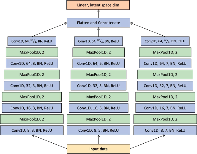
Figure A 1: Architecture of the encoder of the VAE models.

References

- Hinton et al. [2006] Geoffrey E Hinton, Simon Osindero, and Yee-Whye Teh. A fast learning algorithm for deep belief nets. Neural Computation, 18(7):1527–1554, 2006.
- Bengio et al. [2006] Yoshua Bengio, Pascal Lamblin, Dan Popovici, and Hugo Larochelle. Greedy layer-wise training of deep networks. Advances in Neural Information Processing Systems, 19, 2006.
- LeCun et al. [2015] Yann LeCun, Yoshua Bengio, and Geoffrey Hinton. Deep learning. Nature, 521(7553):436–444, 2015.
- Goodfellow et al. [2016] Ian Goodfellow, Yoshua Bengio, and Aaron Courville. Deep Learning. MIT Press, 2016.
- Witten et al. [2017] Ian H Witten, Eibe Frank, Mark A Hall, and Christopher J Pal. Data Mining: Practical Machine Learning Tools and Techniques. Elsevier Inc., 4 edition, 2017.
- Dayan and Abbott [2005] Peter Dayan and Laurence F Abbott. Theoretical Neuroscience: Computational and Mathematical Modeling of Neural Systems. MIT Press, 2005.
- Hinton et al. [1995] Geoffrey E Hinton, Peter Dayan, Brendan J Frey, and Radford M Neal. The" wake-sleep" algorithm for unsupervised neural networks. Science, 268(5214):1158–1161, 1995.
- Vincent et al. [2008] Pascal Vincent, Hugo Larochelle, Yoshua Bengio, and Pierre-Antoine Manzagol. Extracting and composing robust features with denoising autoencoders. In Proceedings of the 25th International Conference on Machine Learning, pages 1096–1103, 2008.
- Goodfellow et al. [2020] Ian Goodfellow, Jean Pouget-Abadie, Mehdi Mirza, Bing Xu, David Warde-Farley, Sherjil Ozair, Aaron Courville, and Yoshua Bengio. Generative adversarial networks. Communications of the ACM, 63(11):139–144, 2020.
- Kingma and Welling [2013] Diederik P Kingma and Max Welling. Auto-encoding variational Bayes. arXiv preprint arXiv:1312.6114, 2013.
- Hinton and Salakhutdinov [2006] Geoffrey E Hinton and Ruslan R Salakhutdinov. Reducing the dimensionality of data with neural networks. Science, 313(5786):504–507, 2006.
- Burda et al. [2015] Yuri Burda, Roger Grosse, and Ruslan Salakhutdinov. Importance weighted autoencoders. arXiv preprint arXiv:1509.00519, 2015.
- Kingma et al. [2014] Durk P Kingma, Shakir Mohamed, Danilo Jimenez Rezende, and Max Welling. Semi-supervised learning with deep generative models. Advances in Neural Information Processing Systems, 27, 2014.
- Jang et al. [2016] Eric Jang, Shixiang Gu, and Ben Poole. Categorical reparameterization with Gumbel-softmax. arXiv preprint arXiv:1611.01144, 2016.
- Maaløe et al. [2017] Lars Maaløe, Marco Fraccaro, and Ole Winther. Semi-supervised generation with cluster-aware generative models. arXiv preprint arXiv:1704.00637, 2017.
- Rolfe [2016] Jason Tyler Rolfe. Discrete variational autoencoders. arXiv preprint arXiv:1609.02200, 2016.
- Vahdat et al. [2018a] Arash Vahdat, William Macready, Zhengbing Bian, Amir Khoshaman, and Evgeny Andriyash. DVAE++: Discrete variational autoencoders with overlapping transformations. In International Conference on Machine Learning, pages 5035–5044. PMLR, 2018a.
- Vahdat et al. [2018b] Arash Vahdat, Evgeny Andriyash, and William Macready. DVAE#: Discrete variational autoencoders with relaxed Boltzmann priors. Advances in Neural Information Processing Systems, 31, 2018b.
- Khoshaman et al. [2019] Amir Khoshaman, Walter Vinci, Brandon Denis, Evgeny Andriyash, Hossein Sadeghi, and Mohammad H Amin. Quantum variational autoencoder. Quantum Science and Technology, 4:014001, 2019.
- Khoshaman and Amin [2018] Amir H Khoshaman and Mohammad Amin. Gumbolt: Extending Gumbel trick to Boltzmann priors. Advances in Neural Information Processing Systems, 31, 2018.
- Vinci et al. [2020] Walter Vinci, Lorenzo Buffoni, Hossein Sadeghi, Amir Khoshaman, Evgeny Andriyash, and Mohammad Amin. A path towards quantum advantage in training classical deep generative models with quantum annealers. Machine Learning: Science and Technology, 1:045028, 2020.
- Vahdat et al. [2020] Arash Vahdat, Evgeny Andriyash, and William Macready. Undirected graphical models as approximate posteriors. In International Conference on Machine Learning, pages 9680–9689. PMLR, 2020.
- An and Cho [2015] Jinwon An and Sungzoon Cho. Variational autoencoder based anomaly detection using reconstruction probability. Special Lecture on IE, 2(1):1–18, 2015.
- Xu et al. [2018] Haowen Xu, Wenxiao Chen, Nengwen Zhao, Zeyan Li, Jiahao Bu, Zhihan Li, Ying Liu, Youjian Zhao, Dan Pei, Yang Feng, et al. Unsupervised anomaly detection via variational auto-encoder for seasonal KPIs in web applications. In Proceedings of the 2018 World Wide Web Conference, pages 187–196, 2018.
- Chen et al. [2019] Run-Qing Chen, Guang-Hui Shi, Wan-Lei Zhao, and Chang-Hui Liang. Sequential VAE-LSTM for anomaly detection on time series. arXiv preprint arXiv:1910.03818, 2019.
- Wang et al. [2020] Xuhong Wang, Ying Du, Shijie Lin, Ping Cui, Yuntian Shen, and Yupu Yang. adVAE: A self-adversarial variational autoencoder with Gaussian anomaly prior knowledge for anomaly detection. Knowledge-Based Systems, 190:105187, 2020.
- Zhang and Chen [2019] Chunkai Zhang and Yingyang Chen. Time series anomaly detection with variational autoencoders. arXiv preprint arXiv:1907.01702, 70, 2019.
- Zhang et al. [2019] Chuxu Zhang, Dongjin Song, Yuncong Chen, Xinyang Feng, Cristian Lumezanu, Wei Cheng, Jingchao Ni, Bo Zong, Haifeng Chen, and Nitesh V Chawla. A deep neural network for unsupervised anomaly detection and diagnosis in multivariate time series data. In Proceedings of the AAAI Conference on Artificial Intelligence, volume 33, pages 1409–1416, 2019.
- Park et al. [2018] Daehyung Park, Yuuna Hoshi, and Charles C Kemp. A multimodal anomaly detector for robot-assisted feeding using an LSTM-based variational autoencoder. IEEE Robotics and Automation Letters, 3(3):1544–1551, 2018.
- Su et al. [2019] Ya Su, Youjian Zhao, Chenhao Niu, Rong Liu, Wei Sun, and Dan Pei. Robust anomaly detection for multivariate time series through stochastic recurrent neural network. In Proceedings of the 25th ACM SIGKDD International Conference on Knowledge Discovery & Data Mining, pages 2828–2837, 2019.
- Memarzadeh et al. [2020] Milad Memarzadeh, Bryan Matthews, and Ilya Avrekh. Unsupervised anomaly detection in flight data using convolutional variational auto-encoder. Aerospace, 7(8):115, 2020.
- Smolensky [1986] Paul Smolensky. Information processing in dynamical systems: Foundations of harmony theory. Technical report, Colorado Univ at Boulder Dept of Computer Science, 1986.
- Kingma and Welling [2019] Diederik P Kingma and Max Welling. An introduction to variational autoencoders. Foundations and Trends® in Machine Learning, 12(4):307–392, 2019.
- Welling et al. [2004] Max Welling, Michal Rosen-Zvi, and Geoffrey E Hinton. Exponential family harmoniums with an application to information retrieval. Advances in Neural Information Processing Systems, 17, 2004.
- Salakhutdinov et al. [2007] Ruslan Salakhutdinov, Andriy Mnih, and Geoffrey Hinton. Restricted Boltzmann machines for collaborative filtering. In Proceedings of the 24th International Conference on Machine learning, pages 791–798, 2007.
- Hinton [2012] Geoffrey E Hinton. A practical guide to training restricted Boltzmann machines. In Neural Networks: Tricks of the Trade, pages 599–619. Springer, 2012.
- Fischer and Igel [2014] Asja Fischer and Christian Igel. Training restricted Boltzmann machines: An introduction. Pattern Recognition, 47(1):25–39, 2014.
- Hinton [2002] Geoffrey E Hinton. Training products of experts by minimizing contrastive divergence. Neural Computation, 14(8):1771–1800, 2002.
- Tieleman [2008] Tijmen Tieleman. Training restricted Boltzmann machines using approximations to the likelihood gradient. In Proceedings of the 25th International Conference on Machine Learning, pages 1064–1071, 2008.
- Tieleman and Hinton [2009] Tijmen Tieleman and Geoffrey Hinton. Using fast weights to improve persistent contrastive divergence. In Proceedings of the 26th Annual International Conference on Machine Learning, pages 1033–1040, 2009.
- Higgins et al. [2017] Irina Higgins, Loic Matthey, Arka Pal, Christopher Burgess, Xavier Glorot, Matthew Botvinick, Shakir Mohamed, and Alexander Lerchner. beta-VAE: Learning basic visual concepts with a constrained variational framework. In Proceedings of the International Conference on Learning Representations, pages 24–26. ICLR, 2017.
- Mnih and Gregor [2014] Andriy Mnih and Karol Gregor. Neural variational inference and learning in belief networks. In International Conference on Machine Learning, pages 1791–1799. PMLR, 2014.
- Paisley et al. [2012] John Paisley, David Blei, and Michael Jordan. Variational Bayesian inference with stochastic search. arXiv preprint arXiv:1206.6430, 2012.
- Gu et al. [2015] Shixiang Gu, Sergey Levine, Ilya Sutskever, and Andriy Mnih. MuProp: Unbiased backpropagation for stochastic neural networks. arXiv preprint arXiv:1511.05176, 2015.
- Bengio et al. [2013] Yoshua Bengio, Nicholas Léonard, and Aaron Courville. Estimating or propagating gradients through stochastic neurons for conditional computation. arXiv preprint arXiv:1308.3432, 2013.
- Maddison et al. [2016] Chris J Maddison, Andriy Mnih, and Yee Whye Teh. The concrete distribution: A continuous relaxation of discrete random variables. arXiv preprint arXiv:1611.00712, 2016.
- Song and Kingma [2021] Yang Song and Diederik P Kingma. How to train your energy-based models. arXiv preprint arXiv:2101.03288, 2021.
- Amin et al. [2018] Mohammad H Amin, Evgeny Andriyash, Jason Rolfe, Bohdan Kulchytskyy, and Roger Melko. Quantum Boltzmann machine. Physical Review X, 8(2):021050, 2018.
- Paszke et al. [2019] Adam Paszke, Sam Gross, Francisco Massa, Adam Lerer, James Bradbury, Gregory Chanan, Trevor Killeen, Zeming Lin, Natalia Gimelshein, Luca Antiga, et al. PyTorch: An imperative style, high-performance deep learning library. Advances in Neural Information Processing Systems, 32, 2019.
- Kingma and Ba [2014] Diederik P Kingma and Jimmy Ba. Adam: A method for stochastic optimization. arXiv preprint arXiv:1412.6980, 2014.
- Li et al. [2021] Yuening Li, Zhengzhang Chen, Daochen Zha, Kaixiong Zhou, Haifeng Jin, Haifeng Chen, and Xia Hu. AutoOD: Neural architecture search for outlier detection. In 2021 IEEE 37th International Conference on Data Engineering (ICDE), pages 2117–2122. IEEE, 2021.
- Du and Mordatch [2019] Yilun Du and Igor Mordatch. Implicit generation and modeling with energy based models. Advances in Neural Information Processing Systems, 32, 2019.
- Sønderby et al. [2016] Casper Kaae Sønderby, Tapani Raiko, Lars Maaløe, Søren Kaae Sønderby, and Ole Winther. Ladder variational autoencoders. Advances in Neural Information Processing Systems, 29, 2016.
- Loaiza-Ganem and Cunningham [2019] Gabriel Loaiza-Ganem and John P Cunningham. The continuous Bernoulli: Fixing a pervasive error in variational autoencoders. Advances in Neural Information Processing Systems, 32, 2019.
- LeCun [1998] Yann LeCun. The mnist database of handwritten digits. http://yann.lecun.com/exdb/mnist/, 1998.
- Federal Aviation Administration [2004] Federal Aviation Administration. Flight operational quality assurance. https://www.faa.gov/documentLibrary/media/ Advisory_Circular/AC_12082.pdf, 120-82, 2004.
- Dillman et al. [2015] Brian G Dillman, Dennis Wilt, Shawn Pruchnicki, Mark Ball, and Marshall Pomeroy. Flight operational quality assurance (FOQA)–do exceedances tell the story? In 18th International Symposium on Aviation Psychology, page 354, 2015.
- Soenen et al. [2021] Jonas Soenen, Elia Van Wolputte, Lorenzo Perini, Vincent Vercruyssen, Wannes Meert, Jesse Davis, and Hendrik Blockeel. The effect of hyperparameter tuning on the comparative evaluation of unsupervised anomaly detection methods. In Proceedings of the KDD’21 Workshop on Outlier Detection and Description, pages 1–9. Outlier Detection and Description Organising Committee, 2021.
- Antoniadis et al. [2022] Ioannis Antoniadis, Vincent Vercruyssen, and Jesse Davis. Systematic evaluation of CASH search strategies for unsupervised anomaly detection. In Fourth International Workshop on Learning with Imbalanced Domains: Theory and Applications, pages 8–22. PMLR, 2022.
- Fu [2006] Michael C Fu. Gradient estimation. In Shane G. Henderson and Barry L. Nelson, editors, Handbooks in Operations Research and Management Science, pages 575–616. Elsevier, 2006.
- Williams [1992] Ronald J Williams. Simple statistical gradient-following algorithms for connectionist reinforcement learning. Machine Learning, 8(3):229–256, 1992.
- Glynn [1990] Peter W Glynn. Likelihood ratio gradient estimation for stochastic systems. Communications of the ACM, 33(10):75–84, 1990.
- Grathwohl et al. [2017] Will Grathwohl, Dami Choi, Yuhuai Wu, Geoffrey Roeder, and David Duvenaud. Backpropagation through the void: Optimizing control variates for black-box gradient estimation. arXiv preprint arXiv:1711.00123, 2017.
- Kuhn and Tucker [1951] HW Kuhn and AW Tucker. Nonlinear programming. In Proceedings of 2nd Berkeley Symposium, pages 481–492, 1951.
- Karush [1939] William Karush. Minima of functions of several variables with inequalities as side constraints. M.Sc. Dissertation. Dept. of Mathematics, Univ. of Chicago, 1939.