Fidelity Out-of-Time-Order Correlator in the Spin-Boson Model

Abstract

In this article, using the numerically exact time-evolving matrix product operators method, we study the fidelity out-of-time-order correlator (FOTOC) in the unbiased spin-boson model at zero temperature. It is found that after the initial exponential growth of FOTOC, the information of the system dynamics will adulterate into the FOTOC. This makes the FOTOC an advanced epitome of the system dynamics, i.e., the FOTOC shows similar behavior to that of system dynamics within a shorter time interval. Eventually the progress of the FOTOC is ahead of the system dynamics, which can provide a prediction of the system dynamics.

I Introduction

The out-of-time-order correlator (OTOC), which was first introduced in the vertex correction of a current in a superconductor Larkin and Ovchinnikov (1969) in 1960s, is recently proposed as a quantum generalization of a classical measure of chaos and to describe quantum information scrambling in a quantum system Li et al. (2017); Hashimoto et al. (2017); Shen et al. (2017); Syzranov et al. (2018); García-Mata et al. (2018); Swingle (2018); Gärttner et al. (2018); Alavirad and Lavasani (2019); Yan and Sinitsyn (2020); Harrow et al. (2021); Zonnios et al. (2022). Recently, it is shown that fidelity OTOC (FOTOC), a specific family of OTOC, can provide profound insight on quantum scrambling behavior. This particular type of OTOC has been considered for studying the multiple quantum coherence spectrum Gärttner et al. (2017, 2018), for quantifying scrambling in Dicke model Lewis-Swan et al. (2019) and quantum Rabi model Kirkova et al. (2022).

The Dicke model Dicke (1954) and quantum Rabi model, which describe the coupling between spin(s) and a single oscillator mode, are fundamental models in quantum optics. In condensed matter physics, there is a fundamental model known as the spin-boson model Leggett et al. (1987); Weiss (1993). The spin-boson model is similar to the Dicke and quantum Rabi models in the sense that it also describes the coupling between a spin and oscillator modes. The difference is that in the spin-boson model, the spectrum of oscillator frequencies is sufficiently dense such that it can be treated continuous and smooth. The presence of continuous modes means that the consideration of recurrence phenomena, which is known to be important in a quantum Rabi like model Eberly et al. (1980), is excluded.

In this article, using an extension of numerically exact time-evolving matrix product operators (TEMPO) method Strathearn et al. (2018); Chen (2023), we calculate the FOTOCs in the unbiased spin-boson model in (sub)ohmic regime at zero temperature. With continuous oscillator modes, the FOTOCs always display exponential deviation from unity at the very beginning of the evolution when the system and bath starting to be entangled. The speed of the deviation is proportional to the square of the system-bath coupling strength. That is, with the same bath the FOTOCs coincides within a very short time despite a factor involving coupling strength factor. Soon after the information of the system dynamics is adulterated into the FOTOCs, which makes them deviates from each other. As the evolution goes on, the FOTOC would contain enough information of the system dynamics and form an advanced epitome of the system dynamics.

This article is organized as follows. The definition of the FOTOC and the model is introduced in Sec. II. The method is presented in Sec. III. The FOTOCs beyond and within the scrambling time are discussed in Sec. V and Sec. IV, respectively. Finally conclusions are given in Sec. VI.

II Fidelity Out-of-Time-Order Correlator in the Spin-Boson Model

Here we consider the unbiased spin-boson model Leggett et al. (1987); Weiss (1993) ($\hbar=1,k_{B}=1$), whose Hamiltonian is given by

$$\begin{split}\hat{H}=&\hat{H}_{S}+\hat{H}_{B}+\hat{H}_{SB}\\ =&\frac{\Delta}{2}\hat{\sigma}_{x}+\sum_{k}\omega_{k}\hat{b}^{{\dagger}}_{k}\hat{b}_{k}+\frac{\hat{\sigma}_{z}}{2}\sum_{k}g_{k}(\hat{b}^{{\dagger}}_{k}+\hat{b}_{k}),\end{split}$$ (1)

here $\Delta$ is the tunneling splitting and $\hat{\sigma}_{x/z}$ are the Pauli matrices. Here $\hat{b}^{{\dagger}}_{k}$ ($\hat{b}_{k}$) creates (annihilates) a boson of state $k$ in bath with frequency $\omega_{k}$, which are coupled to the spin via coupling constant $g_{k}$. The bath is characterized by a spectral function

$$J(\omega)=\sum_{k}g_{k}^{2}\delta(\omega-\omega_{k})=2\alpha\omega^{s}\omega_{c}^{1-s}e^{-\omega/\omega_{c}},$$ (2)

where $\alpha$ is the coupling strength parameter and $\omega_{c}$ is the cutoff frequency of the bath. Here we consider the (sub-)ohmic case where $0<s\leq 1$ and a high frequency cutoff $\omega_{c}=10\Delta$ unless specified otherwise.

The out-of-time-order correlator (OTOC)

$$\mathcal{F}(t)=\langle\hat{W}^{{\dagger}}(t)\hat{V}^{{\dagger}}\hat{W}(t)\hat{V}\rangle$$ (3)

can be served as a diagnostic of quantum chaos, where the brackets denote averaging over the initial state $\ket{\psi_{0}}$. Here $\hat{W}$ and $\hat{V}$ are two initially commuting and Hermitian operators, and $\hat{W}(t)=e^{i\hat{H}t}\hat{W}e^{-i\hat{H}t}$. The OTOCs quantify the degree that $\hat{W}(t)$ and $\hat{V}$ fail to commute at later times due to the time evolution. In fast scramblers, the quantity $1-\real\mathcal{F}(t)$ features an exponential growth for which $1-\real\mathcal{F}(t)\approx e^{\lambda_{Q}t}$ before it saturates. The quantity $\lambda_{Q}$ is the quantum Lyapunov exponent associated with quantum chaos.

In this article, we focus on the so-called fidelity OTOC (FOTOC) where $\hat{V}$ is the projection operator onto the initial state $\ket{\psi}$, i.e., $\hat{V}=\hat{\rho}(0)=\outerproduct{\psi}{\psi}$ and $\hat{W}=e^{i\xi\hat{A}}$ to be a small perturbation ($\xi\ll 1$) for a Hermitian operator $\hat{A}$. For a pure initial state, we have $\mathcal{F}(t)=|\bra{\phi}{\hat{W}(t)}\ket{\phi}|^{2}$.

The FOTOC $\mathcal{F}(t)$ is a real quantity, therefore we write $1-\mathcal{F}(t)$ instead of $1-\real\mathcal{F}(t)$. Expanding $\mathcal{F}(t)$ in a power series of $\xi$ to the second order yields

$$1-\mathcal{F}(t)=\xi^{2}(\langle\hat{A}^{2}(t)\rangle-\langle\hat{A}(t)\rangle^{2})=\xi^{2}\mathrm{var}[\hat{A}(t)],$$ (4)

where $\mathrm{var}[\hat{A}(t)]$ is the variance of $\hat{A}(t)$. This relation connects the exponential growth of quantum variances and quantum chaos.

In Dicke Lewis-Swan et al. (2019) and quantum Rabi Kirkova et al. (2022) model, the bath consists of a single mode boson and the operator $\hat{A}$ is set to be proportional to $(\hat{b}+\hat{b}^{{\dagger}})$. In our spin-boson model, the bath consists of a continuous spectrum of bosons, we chose the corresponding operator to be $\hat{A}=\sum_{k}g_{k}(\hat{b}_{k}+\hat{b}^{{\dagger}}_{k})$. The initial state is $\ket{\psi}=\ket{+,0}$, where the spin is in up state ($\hat{\sigma}_{z}\ket{+,0}=\ket{+,0}$) and the bath is in its ground state.

III Method

At the initial time, the total density matrix is in a product form as $\hat{\rho}(0)=\hat{\rho}_{S}(0)\hat{\rho}_{B}(0)$, where $\hat{\rho}_{S}(0)$ is the initial system density matrix and $\hat{\rho}_{B}(0)$ is the bath density matrix. The bath is in its ground state, i.e., at zero temperature. With such a product initial state, the reduced dynamics of the system at a later time $\hat{\rho}_{S}(t)=\Tr_{B}[\hat{\rho}(t)]$ can be formulated as a path integral via tracing out the bath Feynman and Vernon (1963); Weiss (1993); Grabert et al. (1988); Negele and Orland (1998); Chen (2023). Let $\sigma(\tau)$ be the spin path along a Keldysh contour $\mathcal{C}$ Keldysh (1965); Lifshitz and Pitaevskii (1981); Kamenev and Levchenko (2009); Wang et al. (2013) evolving forward from time $0$ to $t$ then evolving backward to $0$, then we can write

$$\hat{\rho}_{S}(t)=\int\mathcal{D}[\sigma(\tau)]K[\sigma(\tau)]I[\sigma(\tau)],$$ (5)

where the integral over $\mathcal{D}[\sigma(\tau)]$ means summation over all possible paths. Here $K[\sigma(\tau)]$ is the free system propagator and $I[\sigma(\tau)]$ is the Feynman-Vernon influence functional which captures the effects of the bath on the system.

The contour-ordered Green’s function of the free bath is defined as $G_{k}(\tau^{\prime},\tau^{\prime\prime})=\langle T_{\mathcal{C}}\hat{b}_{k}(\tau^{\prime})\hat{b}^{{\dagger}}_{k}(\tau^{\prime\prime})\rangle$, where $T_{\mathcal{C}}$ is the contour-ordering operator. Let $G_{\omega}(\tau^{\prime},\tau^{\prime\prime})$ denote the Green’s function $G_{k}(\tau^{\prime},\tau^{\prime\prime})$ when $\omega_{k}=\omega$, then the influence functional can be written as

$$I[\sigma(\tau)]=e^{-\int_{\mathcal{C}}\differential{\tau^{\prime}}\int_{\mathcal{C}}\differential{\tau^{\prime\prime}}\sigma(\tau^{\prime})\varGamma(\tau^{\prime},\tau^{\prime\prime})\sigma(\tau^{\prime\prime})},$$ (6)

where

$$\varGamma(\tau^{\prime},\tau^{\prime\prime})=\int\differential{\omega}J(\omega)G_{\omega}(\tau^{\prime},\tau^{\prime\prime}).$$ (7)

The quantity $\langle\hat{W}(t)\rangle$ can be obtained from a modified reduced density matrix

$$\hat{\rho}^{\xi}_{S}(t)=\Tr_{B}[\hat{\rho}(t)e^{i\xi\hat{A}}]$$ (8)

via $\langle\hat{W}(t)\rangle=\Tr_{S}\hat{\rho}_{S}^{\xi}$. This modified reduced density matrix can be represented as a path integral for which

$$\hat{\rho}^{\xi}_{S}(t)=\int\mathcal{D}[\sigma(\tau)]K[\sigma(\tau)]I[\sigma(\tau)]X_{\xi}[\sigma(\tau)],$$ (9)

where

$$X_{\xi}[\sigma(\tau)]=e^{\xi\int_{\mathcal{C}}\differential{\tau}[\sigma(\tau)\varGamma(\tau,t^{-})+\varGamma(t^{+},\tau)\sigma(\tau)]}.$$ (10)

Here $t^{\pm}$ means time $t$ on the forward (backward) branch of contour $\mathcal{C}$.

Depending on the parameters on the forward or backward branch, the contour-ordered Green’s function $G_{k}(\tau^{\prime},\tau^{\prime\prime})$ can be split into four blocks $G_{k}^{\pm\pm}(t^{\prime},t^{\prime\prime})$. By doing this we bring the influence functional $I[\sigma(\tau)]$ into normal time axis as $I[\sigma^{\pm}(t)]$. Similarly, the function $\varGamma(\tau^{\prime},\tau^{\prime\prime})$ can be also split into four blocks $\varGamma^{\pm\pm}(t^{\prime},t^{\prime\prime})$, and the quantity $X_{\xi}[\sigma(\tau)]$ can be written in normal time axis as $X_{\xi}[\sigma^{\pm}(t)]$.

For numerical evaluation, the influence functional can be discretized via quasi-adiabatic path-integral (QUAPI) method Makarov and Makri (1993); Makri (1995); Dattani et al. (2012). Split $t$ into $N$ pieces for which $t=N\delta t$ and the path $\sigma^{\pm}(t)$ into intervals of equal duration for which $\sigma^{\pm}(t^{\prime})=\sigma^{\pm}_{j}$ for $(j-\frac{1}{2})\delta t<t^{\prime}<(j+\frac{1}{2}\delta t)$. This splitting corresponds to first order Trotter-Suzuki decomposition Trotter (1959); Suzuki (1976) whose error is about $O(\delta t^{2})$. It is easy to adapt the higher order symmetrized Trotter-Suzuki decomposition Makri (1995); Makri and Makarov (1995); Dattani et al. (2012) which reduces the error to $O(\delta t^{3})$. All the numerical results in this article use the higher order symmetrized decomposition, but for ease of exposition we use the form of first order decomposition. With this splitting, the influence functional $I[\sigma^{\pm}(t)]$ is discretized as

$$I[\quantity{\sigma^{\pm}_{k}}]=e^{-\sum_{j=0}^{N}\sum_{k=0}^{j}(\sigma_{j}^{+}-\sigma_{j}^{-})(\eta_{jk}\sigma_{k}^{+}-\bar{\eta}_{jk}\sigma_{k}^{-})},$$ (11)

where $\eta_{jk}$ is a complex number and $\bar{\eta}_{jk}$ is its complex conjugate. For $j\neq k$ we have

$$\eta_{jk}=\int_{(j-\frac{1}{2})\delta t}^{(j+\frac{1}{2})\delta t}\differential{t^{\prime}}\int_{(k-\frac{1}{2})\delta t}^{(k+\frac{1}{2})\delta t}\differential{t^{\prime\prime}}C(t^{\prime}-t^{\prime\prime}),$$ (12)

and for $j=k$

$$\eta_{jj}=\int_{(j-\frac{1}{2})\delta t}^{(j+\frac{1}{2})\delta t}\differential{t^{\prime}}\int_{(j-\frac{1}{2})\delta t}^{t^{\prime}}\differential{t^{\prime\prime}}C(t^{\prime}-t^{\prime\prime}),$$ (13)

where $C(t)$ is the autocorrelation function.

As mentioned in Ref. Chen (2023), to be consistent with QUAPI method, the variable $\xi$ need to be replaced by a segment as

$$\xi\to\frac{1}{\delta t}\int_{(N-\frac{1}{2})\delta t}^{(N+\frac{1}{2})\delta t}\xi(t^{\prime})\differential{t^{\prime}}$$ (14)

with $\xi(t^{\prime})=\xi$. Therefore $X_{\xi}[\sigma^{\pm}(t)]$ should be discretized as

$$X_{\xi}[\quantity{\sigma^{\pm}_{k}}]=e^{\xi\sum_{j=0}^{N}(\sigma_{j}^{+}\gamma^{+-}_{jN}-\sigma_{j}^{-}\gamma^{--}_{jN}+\gamma^{++}_{Nj}\sigma^{+}_{j}-\gamma^{+-}_{Nj}\sigma^{-}_{j})},$$ (15)

where for $j\neq N$

$$\gamma^{\pm\pm}_{jN}=\frac{1}{\delta t}\int_{(N-\frac{1}{2})\delta t}^{(N+\frac{1}{2})\delta t}\differential{t^{\prime}}\int_{(j-\frac{1}{2})\delta t}^{(j+\frac{1}{2})\delta t}\differential{t^{\prime\prime}}\varGamma^{\pm\pm}(t^{\prime}-t^{\prime\prime}),$$ (16)

and for $j=N$

$$\gamma^{\pm\pm}_{NN}=\frac{1}{\delta t}\int_{(N-\frac{1}{2})\delta t}^{(N+\frac{1}{2})\delta t}\differential{t^{\prime}}\int_{(N-\frac{1}{2})\delta t}^{t^{\prime}}\differential{t^{\prime\prime}}\varGamma^{\pm\pm}(t^{\prime}-t^{\prime\prime}).$$ (17)

The memory time of bath is finite for which $C(t)$ and $\varGamma^{\pm\pm}(t)$ decay to zero for sufficiently large $t$. Therefore the corresponding $\eta_{jk}$ and $\gamma^{\pm\pm}_{jk}$ can be truncated when $\absolutevalue{j-k}$ is larger than a positive integer $\Delta k_{\mathrm{max}}$. This is the key ingredient of QUAPI method, which enables us to simulate the long time evolution of $\hat{\rho}_{S}(t)$ iteratively in a tensor multiplication manner.

The iterative process can be implemented in the language of matrix product state (MPS) and matrix product operator (MPO), which gives a MPS representation of reduced density matrix (5). This yields the so-called time-evolving matrix product operators (TEMPO) algorithm Strathearn et al. (2018). The TEMPO method can employ the standard MPS compression algorithm Schollwöck (2011) during the iterative process, makes it computationally efficient and yet numerically exact. The tensor $X_{\xi}[\quantity{\sigma^{\pm}_{k}}]$ can be easily represented as a MPO, and applying it to the MPS representation of Eq. (5) yields the modified reduced density matrix (9).

In this article, we use the singular value decomposition (SVD) algorithm to compress the MPS. This operation is done by truncating all singular values $\lambda<\varepsilon\lambda_{\mathrm{max}}$, where $\lambda_{\mathrm{max}}$ is the largest singular value and $\varepsilon$ is a convergence parameter. The FOTOC $\mathcal{F}(t)$ is much more numerically sensitive than the polarization $P(t)=\langle\sigma_{z}(t)\rangle$, therefore we need to adopt a fine $\varepsilon=10^{-11}$. The value of perturbation $\xi$ is chosen to be $\xi=10^{-3}$.

IV Beyond the Scrambling Time

Figures 1 and 2 show some typical FOTOCs and corresponding polarizations $P(t)=\langle\hat{\sigma}_{z}(t)\rangle$ in ohmic ($s=1.0$) and subohmic ($s=0.7$) regimes with different coupling strength $\alpha$. The time step is $\delta t=0.1$ in the ohmic case and is $\delta t=0.06$ in the subohmic case. The magnitude of $[1-\mathcal{F}(t)]/\xi^{2}$ roughly scales with $\alpha^{2}$, thus we show the scaled $[1-\mathcal{F}(t)]/\alpha^{2}\xi^{2}$ rather than $[1-\mathcal{F}(t)]/\xi^{2}$. It can be seen that their early behaviors look similar for which all these curves start to grow significantly at the beginning of the evolution and then saturate. After the saturation, they show different long time behaviors.

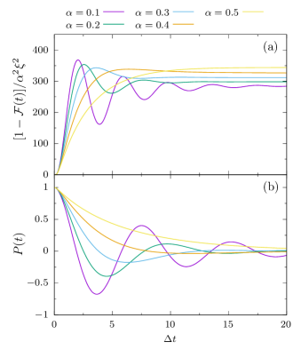
Figure 1: Some typical (a) FOTOCs and (b) polarizations in ohmic $s=1.0$ regime with different coupling strengths.

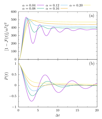
Figure 2: Some typical (a) FOTOCs and (b) polarizations in subohmic $s=0.7$ regime with different coupling strengths.

Usually the scrambling time is identified as the time when $[1-\mathcal{F}(t)]/\alpha^{2}\xi^{2}$ reaches its first local maximum. However, there are some situations, e.g., in Fig. 1(a) the curve just grows monotonically with relatively strong coupling $\alpha=0.5$, where no local maximum can be identified within a short time. In this case, we may roughly identify the scrambling time as the time when the curve decelerates most. Here we try not to identify the scrambling time exactly and just use it as a vague concept to distinguish short and long times. The reason for doing this will be shown in the next section.

It is well known Leggett et al. (1987); Weiss (1993) that at zero temperature, in ohmic regime the polarization $P(t)$ shows damped coherent oscillations with weak coupling and incoherent decay at stronger dissipation, see Fig. 1(b). The transition occurs at $\alpha\approx 0.5$. Similar phenomena happen in the subohmic regime with a smaller transition point $\alpha$, see Fig. 2(b). After the scrambling time, the behaviors of FOTOCs show similarity to the corresponding polarization dynamics in both ohmic (Fig. 1) and subohmic (Fig. 2) regimes. This reminds us that the FOTOCs may contain information of polarization dynamics.

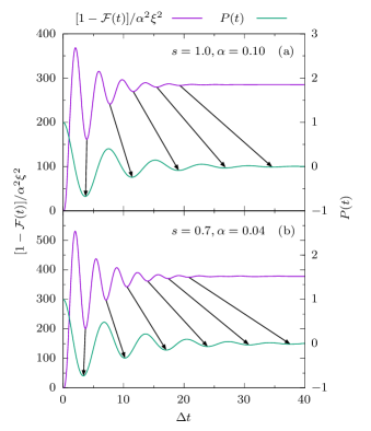
Figure 3: A detailed comparison between the FOTOCs and the polarizations in the ohmic regime. The coupling strength is (a) $\alpha=0.1$ and (b) $\alpha=0.2$.

We choose the ohmic $s=1.0,\alpha=0.1$ [Fig. 3(a)] and the subohmic $s=0.7,\alpha=0.2$ [Fig. 3(b)] cases to demonstrate the similarity between the FOTOCs and the polarizations. We compare the locations of local minimums of the FOTOC and the polarization, and denote the location of $n$th minimum of them as $t_{\mathcal{F}}^{n}$ and $t_{P}^{n}$ respectively.

In Fig. 3(a), the polarization $P(t)$ shows damped coherent oscillation with coupling strength $\alpha=0.1$. Here we compare the first fifth minimums. The first minimums appear at $t_{\mathcal{F}}^{1}=3.9$ and $t_{P}^{1}=3.7$ for which the minimum of polarization is slightly ahead of that of FOTOC. The second minimums appear at $t_{\mathcal{F}}^{2}=7.7$ and $t_{P}^{2}=11.4$ for which polarization is now behind the FOTOC. The rest locations of minimums are $t_{\mathcal{F}}^{3}=11.6,t_{\mathcal{F}}^{4}=15.5,t_{\mathcal{F}}^{5}=19.3$ and $t_{P}^{3}=19.1,t_{P}^{4}=26.84,t_{P}^{5}=34.56$, from which it can be seen that the difference between $t_{\mathcal{F}}^{n}$ and $t_{P}^{n}$ becomes larger along with larger $n$. The time interval between $t_{\mathcal{F}}^{1}$ and $t_{\mathcal{F}}^{5}$ is $15.4$ and that between $t_{P}^{1}$ and $t_{P}^{5}$ is $30.86$, which means the FOTOC go through a similar process with only half the time than polarization.

In Fig. 3(b), the locations of minimums are $t_{\mathcal{F}}^{1}=3.66,t_{\mathcal{F}}^{2}=7.08,t_{\mathcal{F}}^{3}=10.56,t_{\mathcal{F}}^{4}=13.98,t_{\mathcal{F}}^{5}17.4,t_{\mathcal{F}}^{6}=20.76$ and $t_{P}^{1}=3.36,t_{P}^{2}=10.2,t_{P}^{3}=17.04,t_{P}^{4}=23.88,t_{P}^{5}=30.72,t_{P}^{6}=37.56$. The progress of the FOTOC is also behind the polarization at first, then takes the lead at later time. The interval $t_{\mathcal{F}}^{6}-t_{\mathcal{F}}^{1}=17.1$ is also much shorter than $t_{P}^{6}-t_{P}^{1}=34.2$. Therefore we can conclude that the FOTOC forms an epitome of system dynamics, in the sense that it goes through a similar process in a shorter time than system dynamics. In addition, since $t_{\mathcal{F}}^{n}$ is usually ahead of $t_{P}^{n}$ the FOTOC also gives a prediction of the system dynamics.

For large system bath coupling situation, e.g., $\alpha=0.5$ in Fig. 1, the polarization shows incoherent decay and there is no local minimum. In this case, the first local maximum of the corresponding FOTOC disappears and the FOTOC shows incoherent growth. The FOTOC reaches the steady state before the polarization, therefore we may still say that the FOTOC gives an epitome of the polarization.

V Within the Scrambling Time

Let us take a closer look at the FOTOCs within the scrambling time. In Fig. 4, we show the FOTOCs within a very short time with a fine time step $\delta t=0.01$. In the figure, the curves with the same color correspond to various coupling strengths but same $\omega_{c}$.

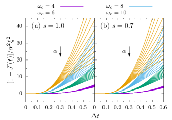
Figure 4: FOTOCs at a short time with different cutoff frequency $\omega_{c}$ and coupling strength $\alpha$ in (a) ohmic ($s=1.0$) regime and (b) subohmic ($s=0.7$) regime. The curves with same color corresponds to same $\omega_{c}$ and the coupling strength is varied from $\alpha=0.1$ to $\alpha=1.0$ by step $0.1$.

It can be seen that with scaling factor $\alpha^{-2}$, the FOTOCs with same $\omega_{c}$ almost coincide at the beginning of the evolution, and then start to deviate soon after. This means that at the very beginning, the dynamics of FOTOCs are irrelevant to the system dynamics and affected most by the environment ($\omega_{c}$), and we may call this part the pure scrambling process. However, soon after the information of the polarization dynamics is adulterated into the FOTOCs which makes them deviate from each other. This deviation happens before the saturation, therefore it is not so appropriate to identify the scrambling time as the location of the first maximum.

The pure scrambling time is hard to be identified since the information of system dynamics is quickly adulterated. This is the reason why we just treat the scrambling time as a vague concept in the previous section. In the beginning, the growth of FOTOCs is fast such that it can be treated as exponential growth. Suppose in pure scrambling process we have $[1-\mathcal{F}(t)]/\xi^{2}\sim e^{\lambda_{Q}t}$, then the coincidence of $[1-\mathcal{F}(t)]/\alpha^{2}\xi^{2}$ indicates that $e^{\lambda_{Q}t}$ is proportional to $\alpha^{2}$, and from which we can deduce that $\lambda_{Q}\sim\ln\alpha$.

VI Conclusions

Using numerically exact time-evolving matrix product operators approach, we study the FOTOC in the unbiased spin-boson model. It is reported that in the Ising chain model, the OTOC will revive and recover unity in the integrable case and oscillates in the nonintegrable case Li et al. (2017). A similar recurrence phenomenon is also reported in quantum Rabi model Kirkova et al. (2022) where the FOTOC oscillates with a certain amplitude. Unlike the quantum Rabi model, the bath in the spin-boson model consists of oscillators of continuous spectrum and thus the consideration of recurrence phenomena is excluded. All FOTOCs in the spin-boson model feature exponential growth initially and eventually remain at some nonzero values. This indicates that the information does scramble in the spin-boson model. Despite a factor $\alpha^{-2}$ the FOTOCs with same $\omega_{c}$ coincide within a very short time. This indicates that the quantum Lyapunov exponent $\lambda_{Q}\sim\ln\alpha$.

After the initial exponential growth process, the information of the system dynamics starts to adulterate into the FOTOCs, which makes them start to deviate from each other before the saturation. After the scrambling time, the FOTOC shows a compressed preview of the system dynamics in the sense that the FOTOC shows similar behavior to that of the system dynamics in a short time. Soon after the progress of FOTOC is ahead of that of the system dynamics, and thus the FOTOC can be used as a prediction of the system dynamics. Therefore we may say that the process of the FOTOCs consists of two subprocesses that one is the information scrambling due to the entanglement of the system and the bath, and another is the adulteration of the information of system dynamics. This two subprocesses compete with each other. The scrambling dominates within a very short time and then it decays to the saturation, and finally the information of system dynamics takes the domination.

References

- Larkin and Ovchinnikov (1969) A. I. Larkin and Y. N. Ovchinnikov, Soviet Physics JETP 28, 1200 (1969).
- Li et al. (2017) J. Li, R. Fan, H. Wang, B. Ye, B. Zeng, H. Zhai, X. Peng, and J. Du, Physical Review X 7, 031011 (2017).
- Hashimoto et al. (2017) K. Hashimoto, K. Murata, and R. Yoshii, Journal of High Energy Physics 2017, 138 (2017).
- Shen et al. (2017) H. Shen, P. Zhang, R. Fan, and H. Zhai, Physical Review B 96, 054503 (2017).
- Syzranov et al. (2018) S. V. Syzranov, A. V. Gorshkov, and V. Galitski, Physical Review B 97, 161114 (2018).
- García-Mata et al. (2018) I. García-Mata, M. Saraceno, R. A. Jalabert, A. J. Roncaglia, and D. A. Wisniacki, Physical Review Letters 121, 210601 (2018).
- Swingle (2018) B. Swingle, Nature Physics 14, 988 (2018).
- Gärttner et al. (2018) M. Gärttner, P. Hauke, and A. M. Rey, Physical Review Letters 120, 040402 (2018).
- Alavirad and Lavasani (2019) Y. Alavirad and A. Lavasani, Physical Review A 99, 043602 (2019).
- Yan and Sinitsyn (2020) B. Yan and N. A. Sinitsyn, Physical Review Letters 125, 040605 (2020).
- Harrow et al. (2021) A. W. Harrow, L. Kong, Z.-W. Liu, S. Mehraban, and P. W. Shor, PRX Quantum 2, 020339 (2021).
- Zonnios et al. (2022) M. Zonnios, J. Levinsen, M. M. Parish, F. A. Pollock, and K. Modi, Physical Review Letters 128, 150601 (2022).
- Gärttner et al. (2017) M. Gärttner, J. G. Bohnet, A. Safavi-Naini, M. L. Wall, J. J. Bollinger, and A. M. Rey, Nature Physics 13, 781 (2017).
- Lewis-Swan et al. (2019) R. J. Lewis-Swan, A. Safavi-Naini, J. J. Bollinger, and A. M. Rey, Nature Communications 10, 1581 (2019).
- Kirkova et al. (2022) A. V. Kirkova, D. Porras, and P. A. Ivanov, Physical Review A 105, 032444 (2022).
- Dicke (1954) R. H. Dicke, Physical Review 93, 99 (1954).
- Leggett et al. (1987) A. J. Leggett, S. Chakravarty, A. T. Dorsey, M. P. A. Fisher, A. Garg, and W. Zwerger, Reviews of Modern Physics 59, 1 (1987).
- Weiss (1993) U. Weiss, Quantum Dissipative Systems (World Scientific, Singapore, 1993).
- Eberly et al. (1980) J. H. Eberly, N. B. Narozhny, and J. J. Sanchez-Mondragon, Physical Review Letters 44, 1323 (1980).
- Strathearn et al. (2018) A. Strathearn, P. Kirton, D. Kilda, J. Keeling, and B. W. Lovett, Nature Communications 9, 3322 (2018).
- Chen (2023) R. Chen, New Journal of Physics (2023), 10.1088/1367-2630/acc60a.
- Feynman and Vernon (1963) R. P. Feynman and F. L. Vernon, Annals of Physics 24, 118 (1963).
- Grabert et al. (1988) H. Grabert, P. Schramm, and G.-L. Ingold, Physics Reports 168, 115 (1988).
- Negele and Orland (1998) J. W. Negele and H. Orland, Quantum Many-Particle Systems (Westview Press, 1998).
- Keldysh (1965) L. V. Keldysh, Soviet Physics JETP 20, 1018 (1965).
- Lifshitz and Pitaevskii (1981) E. M. Lifshitz and L. P. Pitaevskii, Course of Theoretical Physics Volume 10: Physical Kinetics (Elsevier, 1981).
- Kamenev and Levchenko (2009) A. Kamenev and A. Levchenko, Advances in Physics 58, 197 (2009).
- Wang et al. (2013) J.-S. Wang, B. K. Agarwalla, H. Li, and J. Thingna, Frontiers of Physics 9, 673 (2013).
- Makarov and Makri (1993) D. E. Makarov and N. Makri, Physical Review A 48, 3626 (1993).
- Makri (1995) N. Makri, Journal of Mathematical Physics 36, 2430 (1995).
- Dattani et al. (2012) N. S. Dattani, F. A. Pollock, and D. M. Wilkins, Quantum Physics Letters 1, 35 (2012).
- Trotter (1959) H. F. Trotter, Proceedings of the American Mathematical Society 10, 545 (1959).
- Suzuki (1976) M. Suzuki, Communications in Mathematical Physics 51, 183 (1976).
- Makri and Makarov (1995) N. Makri and D. E. Makarov, The Journal of Chemical Physics 102, 4600 (1995).
- Schollwöck (2011) U. Schollwöck, Annals of Physics 326, 96 (2011).