EBSR: Enhanced Binary Neural Network for Image Super-Resolution

Abstract

While the performance of deep convolutional neural networks for image super-resolution (SR) has improved significantly, the rapid increase of memory and computation requirements hinders their deployment on resource-constrained devices. Quantized networks, especially binary neural networks (BNN) for SR have been proposed to significantly improve the model inference efficiency but suffer from large performance degradation. We observe the activation distribution of SR networks demonstrates very large pixel-to-pixel, channel-to-channel, and image-to-image variation, which is important for high performance SR but gets lost during binarization. To address the problem, we propose two effective methods, including the spatial re-scaling as well as channel-wise shifting and re-scaling, which augments binary convolutions by retaining more spatial and channel-wise information. Our proposed models, dubbed EBSR, demonstrate superior performance over prior art methods both quantitatively and qualitatively across different datasets and different model sizes. Specifically, for $\times 4$ SR on Set5 and Urban100, EBSR-light improves the PSNR by 0.31 dB and 0.28 dB compared to SRResNet-E2FIF, respectively, while EBSR outperforms EDSR-E2FIF by 0.29 dB and 0.32 dB PSNR, respectively.

1 Introduction

Image super-resolution (SR) is a classic yet challenging problem in computer vision. It aims to reconstruct high-resolution (HR) images, which have more details and high-frequency information, from low-resolution (LR) images. Image SR is an ill-posed problem as there are multiple HR images corresponding to a single SR image [24]. In recent years, deep neural networks (DNNs) have achieved great quality improvement in image SR but also, suffers from intensive memory consumption and computational cost [11, 13, 29, 28]. The high memory and computation requirements of SR networks hinder their deployment on resource-constrained devices, such as mobile phones and other embedded systems.

Network quantization has been naturally used to compress SR models [12, 6, 30] as an effective way to reduce memory and computation costs while maintaining high accuracy. In network quantization, binary neural networks (BNNs), which quantize activations and weights to $\{-1,1\}$, are of particular interest because of their memory saving by 1-bit parameters and computation saving by replacing convolution with bit-wise operations, including XNOR and bit-count [20]. Ma et al. [16] are the first to introduce binarization to SR networks. However, they only binarize weights and leave activations at full precision, which impedes the bit-wise operation and leads to a limited speedup. Afterward, many works [25, 8, 10] have explored BNNs for image SR with both binary activations and weights. Though promising results have been achieved, all these BNNs still suffer from a large performance degradation compared to the floating point (FP) counterparts.

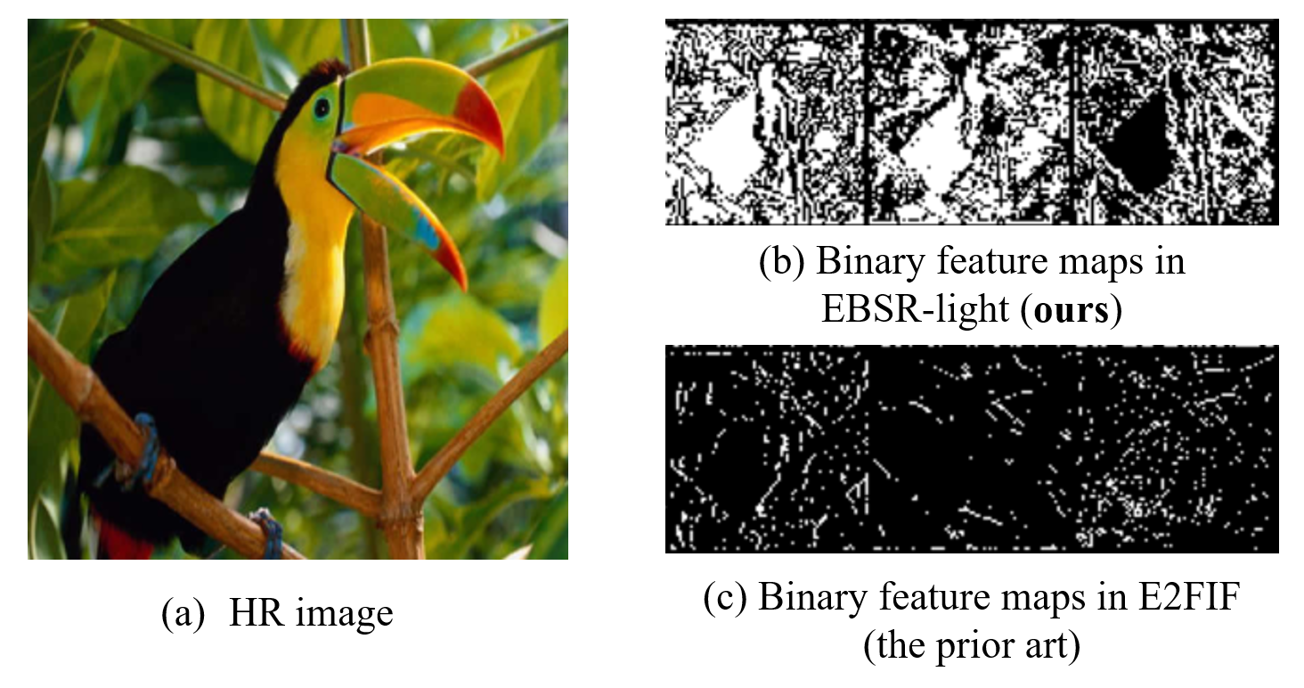
Figure 1: The binary feature maps of the same channels in the same block in our EBSR-light and the prior art E2FIF.

We observe the large performance degradation comes from two reasons. First of all, existing BNNs for SR surprisingly adopt a simple binarization method, which directly applies the sign function to binarize the activations. In contrast, more advanced binarization methods have been demonstrated in BNNs for image classification [14, 1, 18]. Hence, how to improve the binarization methods becomes the first question towards high-performance BNNs for SR.

Secondly, the majority of recent full-precision SR networks [13, 27, 29] remove batch normalization (BN) for better performance. This is because BN layers normalize the features and destroy the original luminance and contrast information of the input image, resulting in blurry output images and worse visual quality [13]. After removing BN, we observe the activation distribution of SR networks exhibits much larger pixel-to-pixel, channel-to-channel, and image-to-image variation, which we hypothesize is important to capture the image details for high performance SR. However, such distribution variation is very unfriendly to BNN. On one hand, it leads to a large binarization error and makes BNN training harder. For the reason, recent works, e.g., E2FIF [10], add the BN back to the BNNs, and thus, suffers from blurry outputs. On the other hand, the variation of activation distribution is very hard to preserve. For example, each activation tensor in the BNN share the same binarization parameters, e.g., scaling factors. This makes it very hard to preserve the magnitude differences across channels and pixels. Hence, how to better capture the distribution variation is the second important question.

Table 1: Comparison between our works and previous BNN in image classification and super-resolution tasks.

Method	Weight	Act	Adaptive Quant	w/ BN	HW Cost	Task
[3]	Per chl	Per tensor	Spatial	Yes	Low	Cls
[18]	Per chl	Per tensor	Chl	Yes	Low	Cls
ReActNet[14]	Per chl	Per tensor	No	Yes	Low	Cls
[16]	Per chl	FP	No	Yes	FP Accum.	SR
BAM [25]	Per tensor	Per tensor	No	Yes	Extra FP BN	SR
BTM [8]	Per chl	Per tensor	No	No	Low	SR
DAQ [6]	Per chl	Per chl	Chl	No	FP Mul. and Accum.	SR
E2FIF [10]	Per chl	Per tensor	No	Yes	Low	SR
[HTML]EFEFEF EBSR (ours)	Per chl	Per tensor	Spatial, chl, and img	No	Low	SR

To address the aforementioned questions, in this paper, we propose EBSR, an enhanced BNN for image SR. EBSR features two important changes over the previous BNNs for SR, including leveraging more advanced binarization methods to stabilize training without BN, and novel methods, including spatial re-scaling as well as channel-wise shifting and re-scaling to better capture the spatial and channel-wise activation distribution. The resulting EBSR binary features can preserve much more textures and details for SR compared to prior art methods as shown in Figure 1. Our contributions can be summarized as below:

• We leverage advanced binarization methods to build a strong BNN baseline, which stabilizes the training without BN and outperforms prior art methods.

• We observe the spatial and channel-wise variation of activation distribution is important for SR quality and propose novel methods to capture the variation, which preserve much more details.

• We evaluate our models on benchmark datasets and demonstrate significant performance improvement over the prior art method, i.e, E2FIF. Specifically, EBSR-light outperforms E2FIF by 0.31 dB and 0.28 dB on Set5 and Urban100, respectively, at $\times 4$ scale at a slight computation increase. EBSR-SQ achieves 0.26 dB and 0.27 dB PSNR improvements over E2FIF at the same computation cost.

2 Related Works

2.1 Image super-resolution deep neural networks

DNNs have been widely used in image SR for their satisfying performance. The pioneering work SRCNN [4] first uses a DNN which has only three convolution layers to reconstruct the HR image in an end-to-end way. VDSR [9] increases the network depth to 20 convolution layers and introduces global residual learning for better performance. SRResNet [11] introduces residual blocks in SR and achieves better image quality. SRGAN [11] uses SRResNet as the generator and an additional discriminator to recover more photo-realistic textures. EDSR [13] removes BN in the residual block and features with a deeper and wider model with up to 43M model parameters. Dense connect [29], channel attention module [27], and non-local attention [28] mechanism are also used in SR networks to improve the image quality. However, these networks have very large memory and computation overheads that can hardly be deployed on resource-constrained devices.

2.2 BNN for image super-resolution

To compress the SR models, BNNs for SR have been studied in recent years. For a BNN, the binarization function can be written as $\hat{x}=\alpha\operatorname{sign}(x-\beta)$, where $\alpha$, $\beta$, $x$ and $\hat{x}$ denote the scaling factor, bias, the FP and binary variables, respectively. There are two kinds of binarization strategies [19], including per-tensor and per-channel binarization. The major difference is per-tensor binarization uses the same $\alpha$ and $\beta$ for the whole tensor while per-channel binarization has channel-wise $\alpha$s and $\beta$s.

We compare different BNNs for SR and for image classification tasks in Table 1. Ma et al. [16] first introduce binarization to SR networks and reduce the model size by $80\%$ compared with FP SRResNet. However, they only binarize weights and leave activations at FP, which impedes the bit-wise operation and requires FP accumulations. Xin et al. [25] binarizes both weights and activations in SR networks utilizing a bit-accumulation mechanism (BAM) to approximate the FP convolution. A value accumulation scheme is proposed to binarize each layer based on all previous layers. However, their method introduces extra FP BN computation during inference. Jiang et al. [8] find that simply removing BN leads to large performance degradation. Hence, they explore a binary training mechanism (BTM) to better initialize weights and normalize input LR images. They build a BNN without BN named IBTM. After that, Hong et al. proposed DAQ[6] adaptive to diverse channel-wise distributions. However, they use per-channel activation quantization which introduces large FP multiplications and accumulations. Recently Lang et al. [10] propose using end-to-end full-precision information flow in BNN and develops a high performance BNN named E2FIF. However, there is a still large gap with the full-precision model. None of the binarization methods above have the ability to capture the pixel-to-pixel, channel-to-channel, and image-to-image variation of the activation distribution.

3 Motivation

To better understand the origin of performance degradation of BNN for SR, in this section, we visualize the activation distributions for a FP SR network. We select a lightweight EDSR model, which has 16 blocks and 64 channels for the body module [13]. We also visualize the activation distribution of a image classification network, i.e., MobileNetV2 [21] for comparison. From the comparison, we observe clear differences between the two models, which serves as the motivation for our EBSR.

((a)) MobileNetV2

((b)) EDSR

Figure 2: Activation distribution of EDSR exhibits much larger pixel-to-pixel variation compared to MobileNetV2.

Motivation 1: Pixel-to-Pixel Variation We first compare the activation distribution for different pixels within the same layer. We randomly sample 24 pixels from one layer of both MobileNetV2 and EDSR and visualize the activation distribution for these pixels in Figure 2. As we can observe, for MobileNetV2, due to BN, the activation distribution of different pixels are very similar to each other with relatively small magnitude. In contrast, for EDSR, on one hand, the magnitude of the activation distribution is much larger compared to MobileNetV2; while on the other hand, the magnitude of different pixels are also quite different. Such phenomenon is not specific to a certain layer in EDSR. According to [3], the difference of activation magnitudes indicates different scaling factors are needed for each pixel. However, per-pixel binarization is not hardware friendly while existing per-tensor binarization schemes cannot capture the pixel-to-pixel variation of activation distribution.

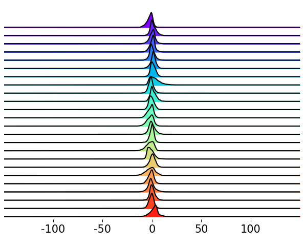
((a)) Image1 in MobileNetV2

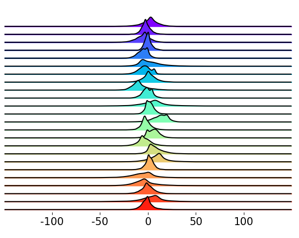
((b)) Image1 in EDSR

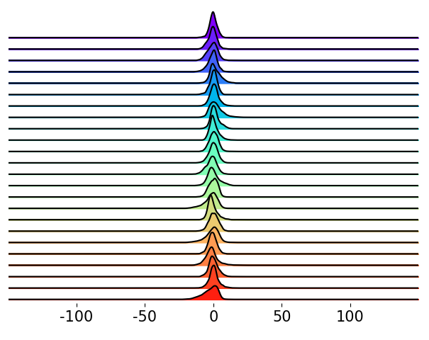
((c)) Image2 in MobileNetV2

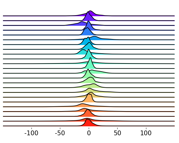
((d)) Image2 in EDSR

Figure 3: Activation distribution of EDSR exhibits much larger channel-to-channel (horizontal view) and image-to-image (vertical view) variations compared to MobileNetV2.

Motivation 2: Channel-to-Channel Variation We now compare the activation distributions for different channels within each layer. We randomly sample 24 channels from the same layer of both MobileNetV2 and EDSR and visualize the activation distribution in Figure 9(b) and 9(c). As we can observe, the activation distribution of EDSR is different from that of MobileNetV2 in that both the mean and variance of activations varies a lot across different channels in EDSR. This indicates different channels require both different scaling factors and different bias during binarization.

One way to resolve the channel-to-channel variation of activation distribution is to leverage per-channel quantization, which is used in [6]. However, per-channel quantization prevents BNN from performing bit-wise operations for convolution, which makes BNN lose its most important advantage. This is illustrated in Figure 4. In this toy example, we have an activation tensor $A\in\mathbb{R}^{1\times 4\times 2\times 2}$ and a weight tensor $W\in\mathbb{R}^{2\times 4\times 1\times 1}$. When we convolve A with the first filter in red color, for activation per-tensor binarization (e.g., Figure 4(a)), the convolution can be calculated as $s_{a}s_{w_{1}}\left[1\times 1+\left(-1\right)\times 1+\left(-1\right)\times 1+1\times 1\right]$, where $\left[\cdot\right]$ can be calculated efficiently by xnor and bit-count operations. However, for activation per-channel binarization (e.g., Figure 4(b)), each channel of activations has a real-valued scaling factor and the convolution is computed as $s_{a_{1}}s_{w_{1}}-s_{a_{2}}s_{w_{1}}+s_{a_{3}}s_{w_{1}}+s_{a_{4}}s_{w_{1}}$, where all terms need to be calculated in FP without any acceleration. Thus activation per-channel binarization is not feasible for BNN.

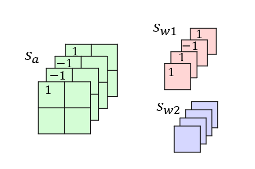
((a)) Activation per-tensor quantize

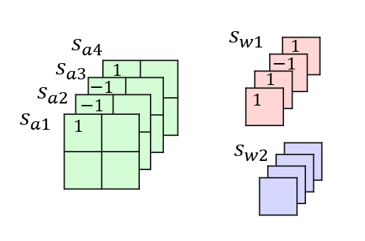
((b)) Activation per-channel quantize

Figure 4: Activation per-channel quantize (a) and per-tensor quantize (b). For weights quantization, both (a) and (b) are per channel, i.e., each channel in the convolution output tensor has different scaling factors, which also means each kernel has a different scaling factor.

Motivation 3: Image-to-Image Variation We further compare the activation distributions of the same layer for different images. As shown in Figure 9(c) and 9(e), for EDSR, both the mean and magnitude of the activation distributions are different, indicating different images may require different scaling factors and bias as well.

Remark For the analysis above, by comparison with MobileNetV2, we observe the activation distribution of EDSR exhibits clear pixel-to-pixel, channel-to-channel, and image-to-image variation. We hypothesize this is important for high quality SR as it captures details specific to different images. To preserve such variation requires the binarization scaling factor to be pixel, channel, and image dependent while requires the bias to be channel and image dependent. How to realize such requirements in BNNs would be important to close the gap with their full-precision counterparts.

4 Build A Strong Baseline

Currently, most BSR networks use the following simple sign function for per-tensor activation binarization and per-channel weight binarization [19]:

$$\hat{x}=\operatorname{sign}(x)\quad\hat{w_{i}}=\frac{\|w_{i}\|_{l1}}{n}\operatorname{sign}(w_{i})$$ (1)

where $\hat{x}$ and $x$ denote the binary and real-valued activation, respectively, $\hat{w_{i}}$ and $w_{i}$ denote the binary weights and real-valued weights, respectively, and $n$ denote the number of weights in the $i_{th}$ weight filter. However, due to the variation of activation distributions, such simple binarization scheme suffers from convergence issue and low performance when the BN is removed. Therefore, we first build a strong baseline BNN based on the robust binarization method and propose a reliable network structure in this section.

4.1 Binarization

To handle the channel-to-channel variation of the activation mean, we first introduce RSign following ReActNet [14], which has a channel-wise learnable threshold. We also adopt a learnable scaling factor for each activation tensor to further reduce the quantization error between binary and real-valued activations. Hence, the binarization function used for activations is defined as:

$$\hat{x}=\alpha\operatorname{sign}(\frac{x-\beta_{i}}{\alpha})$$ (2)

where $\beta_{i}$ is the channel-wise learnable thresholds and $\alpha$ is the learnable scaling factor for each activation tensor. Both of them can be optimized end-to-end with other parameters in the network. To back-propagate the gradients through the discretized binarization function, we follow [15] to use a piecewise polynomial function as the straight-through estimator (STE), which can reduce the gradient mismatch effectively. Thus, the gradient w.r.t. $\alpha$ can be calculated as:

$$\frac{\partial\hat{x}}{\partial\alpha}=\begin{cases}-1,&\text{ if }x\leq\beta-\alpha\\ -2\left(\frac{x-\beta}{\alpha}\right)^{2}-2\frac{x-\beta}{\alpha}-1,&\text{ if }\beta-\alpha<x\leq\beta\\ 2\left(\frac{x-\beta}{\alpha}\right)^{2}-2\frac{x-\beta}{\alpha}+1,&\text{ if }\beta<x\leq\beta+\alpha\\ 1,&\text{ if }x>\beta+\alpha\end{cases}$$ (3)

while the gradient w.r.t. $\beta_{i}$ can be computed as:

$$\frac{\partial\hat{x}}{\partial\beta_{i}}=\begin{cases}-2-2\frac{x-\beta_{i}}{\alpha},&\text{ if }\quad\beta_{i}-\alpha<x\leqslant\beta_{i}\\ -2+2\frac{x-\beta_{i}}{\alpha,},&\text{ if }\beta_{i}<x\leqslant\beta_{i}+\alpha\\ 0,&\text{ otherwise }\end{cases}$$ (4)

For weight binarization, we still use the channel-wise sign function in Eq.1, for which the scaling factors are the average of the $\ell_{1}$ norm of each filter.

4.2 Baseline Network Structure

We use the lightweight EDSR with 16 blocks and 64 channels, and EDSR with 32 blocks and 256 channels as our backbones for two variants namely EBSR-light and EBSR. Following existing BSR networks [16, 25, 8, 10], we only binarize the body module and leave the head and tail modules in full-precision which only contain one convolution layer each. We also follow Bi-Real Net [15] and E2FIF [10] to use a skip connection bypassing every binary convolution layer in order to keep the full-precision information from being cut off by binary layers. Note that the network structure here doesn’t contain BN layers.

Table 2 shows the comparison between our proposed baseline and the prior art E2FIF. As can be observed, for E2FIF, removing BN leads to a huge performance degradation. In contrast, for our strong baseline, its training is stable without BN and it outperforms E2FIF both with and without BN.

Table 2: Comparison between our strong baseline with E2FIF and their counterparts with BN on Set5 and Urban100 at x4 scale.

Models	Set5		Urban100
	PSNR	SSIM	PSNR	SSIM
E2FIF w/ BN	31.270	0.879	25.070	0.748
[HTML]FFFFFF E2FIF w/o BN	29.274	0.827	23.602	0.682
Baseline w/ BN	31.296	0.880	25.090	0.751
[HTML]FFFFFF Baseline	31.301	0.880	25.093	0.751

5 Method

In this section, we propose two techniques to further enhance the strong baseline to capture the variation of activation distributions better. We first introduce spatial re-scaling to adapt the network to pixel-to-pixel variation. We then propose channel-wise shifting and re-scaling to better capture the channel-to-channel variation. Meanwhile, as both of the two methods are image-dependent, the image-to-image variation can be captured naturally. By combining the two methods with our strong baseline, we build our enhanced BNN for SR, named EBSR.

5.1 Spatial Re-scaling

As is shown in Figure 2, activation distributions have large pixel-to-pixel variation in SR networks and the difference of activation magnitudes indicates different scaling factors are preferred for different pixels. Inspired by [18], we propose spatial re-scaling to better adapt the network to the spatial variation of activation distributions in SR networks. We take the real-valued activations $A$ before convolution as input and predict pixel-wise scaling factors $S(A)$, which re-scale the binary convolution output. Spatial re-scaling process can be formulated as follows:

$$A*W\approx(\operatorname{sign}(A)\circledast\operatorname{sign}(W))\odot\alpha\odot S(A)$$ (5)

where $\circledast$ denotes the binary convolution and $\odot$ denotes the element-wise multiplication. $A$, $W$, $\alpha$, and $S\left(A\right)$ denote real-valued activations, weights, the scaling factor of weights, and the spatial-wise scaling factor of activations respectively. $S\left(A\right)\in\mathbb{R}^{1\times H\times W}$ can be calculated with a convolution and a sigmoid function. As shown in Figure 5(a), real-valued activations first go through a convolution layer, which has an input channel of $C$ and an output channel of 1, and then pass through a sigmoid function to produce the scaling factors $S(A)$ along the spatial dimension. During inference, the scaling factor will change dynamically according to different input feature maps. By re-scaling binary convolution output using $S(A)$, we can reduce the quantization error and the original pixel-wise information in FP activation will be preserved much better. Spatial re-scaling leads to a large PSNR improvement of 0.24 dB (from 30.30 dB to 31.54 dB) on Set5 and 0.22 dB (from 25.09 dB to 25.31 dB) on Urban100 compared with our strong baseline.

5.2 Channel-wise Shifting and Re-scaling

Table 3: Comparison between whether to fuse channel-wise shifting and re-scaling or not based on our baseline with spatial re-scaling.

Method	OPs	Params	Set5		Urban100
			PSNR	SSIM	PSNR	SSIM
Baseline + spatial re-scale	2.16G	0.05M	31.54	0.883	25.31	0.759
+ channel-wise shift and re-scale	2.34G	0.09M	31.61	0.885	25.35	0.761
+ w/ fusing	2.27G	0.08M	31.64	0.885	25.36	0.761

In SR networks, activation distributions exhibit larger channel-to-channel variation (Figure 3). Both the mean and magnitude of the activation distributions vary significantly across channels. [18] has proposed the data-driven channel re-scaling, but our method differs from them in further introducing data-driven thresholds to handle the channel-wise variation of both mean and magnitude. Since the blocks to generate the scaling factors and thresholds are very similar, we further propose to fuse them into one module. We evaluate the effect of fusing the two blocks in Table 3. With channel-wise shifting and re-scaling fused, our models have fewer operations and parameters overhead and slightly higher performance.

For the specific process, we take the real-valued activations as input and predict different thresholds and scaling factors for each channel. They are also image dependent, e.g., $\beta_{i}$ in Eq.2 is no longer fixed during inference but generated according to different input feature maps. Channel-wise shifting and re-scaling can be formulated as follows:

$$A*W\approx(\operatorname{sign}(A-C_{s}(A))\circledast\operatorname{sign}(W))\odot\alpha\odot C_{r}(A)$$ (6)

where $\circledast$ denotes the binary convolution and $\odot$ denotes the element-wise multiplication. $C_{s}(A),C_{r}(A)\in\mathbb{R}^{C\times 1\times 1}$ denote the channel-wise threshold and scaling factor, respectively. We show the block diagram in Figure 5(b). The real-valued input feature map is first squeezed to a ${C\times 1\times 1}$ vector by a global average pooling (GAP) layer. The subsequent fully connected layers and ReLU learn the channel-wise information and output a ${2C\times 1\times 1}$ vector. Then the ${2C\times 1\times 1}$ vector is split into two ${C\times 1\times 1}$ vectors. We use the first $C$ channels as the channel-wise bias and pass the last $C$ channels through a sigmoid layer as the channel-wise scaling factor, which are used to shift the real-valued activations and re-scale the binary convolution output, respectively.

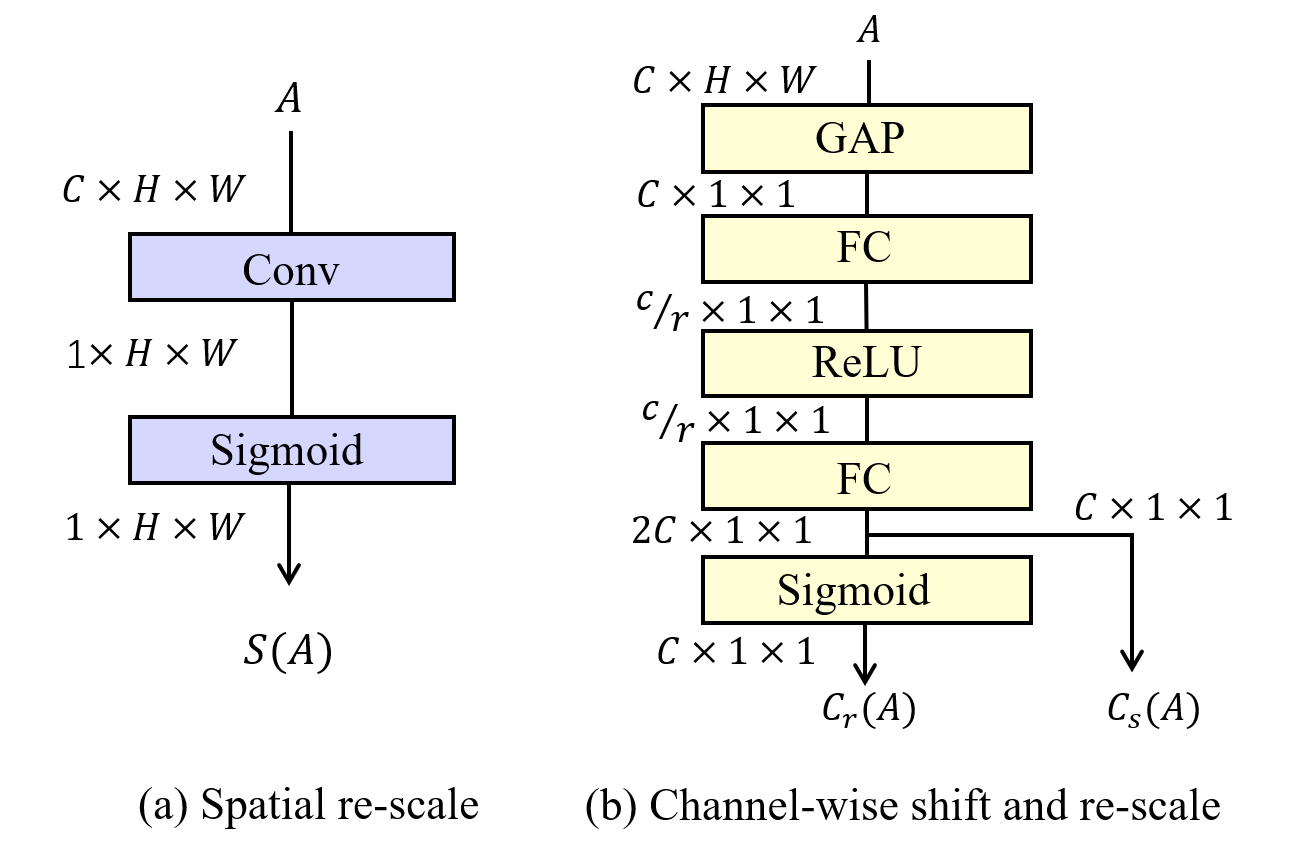
Figure 5: Block diagram for spatial re-scaling, and channel-wise shifting and re-scaling.

5.3 Network Structure

Combining the spatial re-scaling and the channel-wise shifting and re-scaling methods, we construct the enhanced convolution layer (E-Conv). Then we build our EBSR model based on E-Conv. In Figure 6, we compare the binary convolution layer used in the baseline network and our proposed E-Conv. We use spatial and channel-wise scaling factors to re-scale the binary convolution output, and use channel-wise shifting to learn appropriate thresholds for each channel before binarization. The scaling factors and threshold used in E-Conv are learnable and depend on the real-valued input activations. In this way, our proposed EBSR can adapt to pixel-to-pixel, channel-to-channel, and image-to-image variations to reduce the large binarization error and preserve more details.

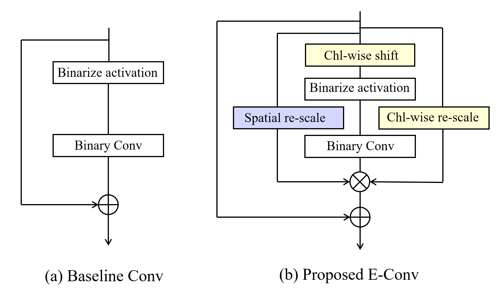
Figure 6: Comparison of (a) the binary convolution layer with a skip connection used in our baseline network and (b) the proposed E-Conv.

Figure 7 shows the basic block based on the E-Conv and our EBSR composed of the basic blocks. Following existing works, the convolution layers in the head and tail modules are not binarized. We choose the lightweight EDSR which has 16 basic blocks and 64 channels, and EDSR which has 32 basic blocks and 256 channels as our backbones, which correspond to EBSR-light and EBSR, respectively.

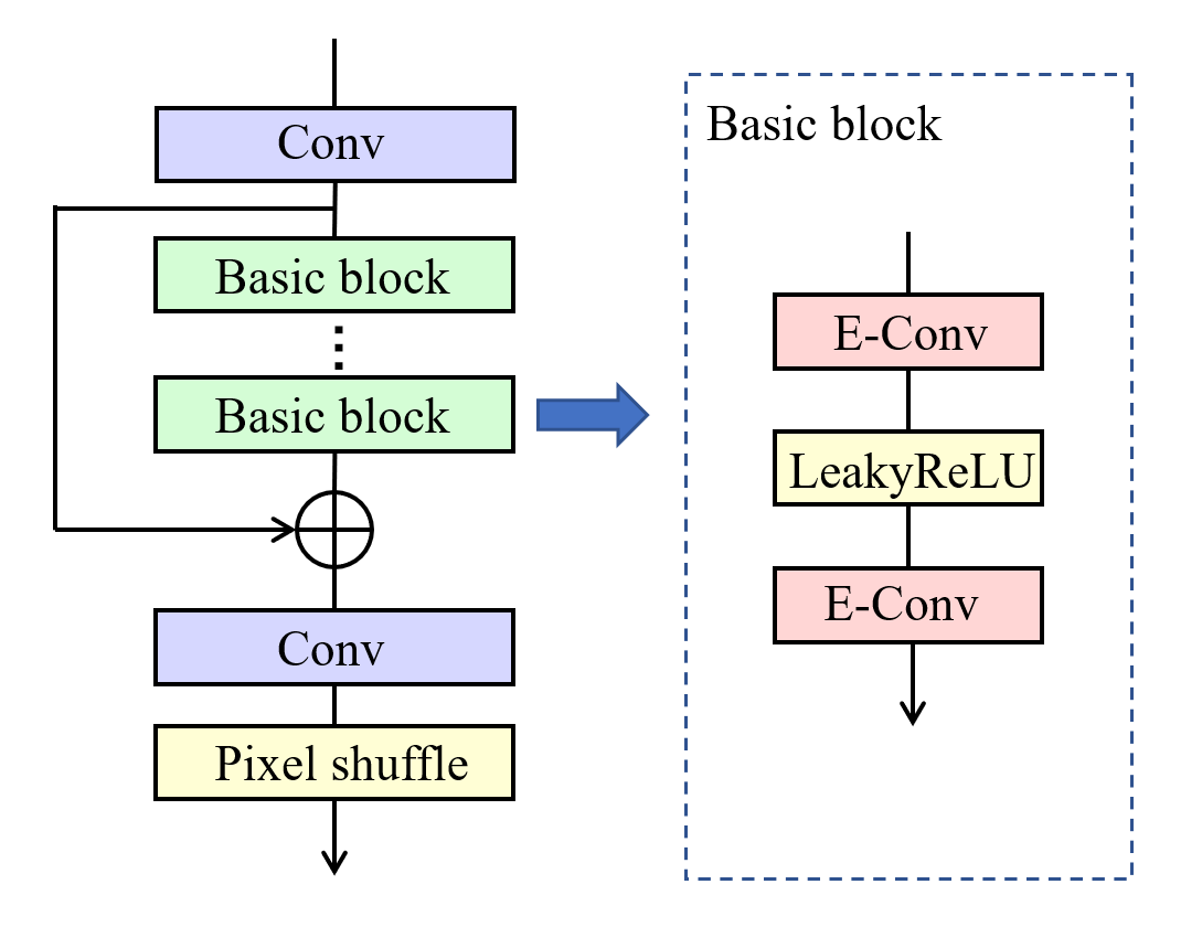
Figure 7: The structure of our proposed EBSR. Convolution layers in purple are real-valued vanilla 3x3 convolutions.

6 Experiments

6.1 Experimental Setup

We train all the models on the training set of DIV2K [22]. Our models operate on RGB channels, i.e., the input and output image are in RGB color space, not YCbCr color space. For evaluation, we use four standard benchmarks including Set5 [2], Set14 [26], B100 [17] and Urban100 [7]. For evaluation metrics, we use PSNR and SSIM [23] over the Y channel between the output SR image and the original HR image as most previous works did.

We choose L1 loss between SR image and HR image [13] as our loss function. Input patch size is set to $48\times 48$. The mini-batch size is set to 16. We use ADAM optimizer with $\beta_{1}=0.9$, $\beta_{2}=0.999$, and $\epsilon=10^{-8}$. The learning rate is initialized as $2\times 10^{-4}$ and halved every 200 epochs. All our models are trained from scratch for 300 epochs.

Table 4: Memory and computation overheads of different models. W and A denote the bit-width of weights and activations in quantized spatial re-scaling module.

Models	OPs	Params	Set5		Urban100
			PSNR	SSIM	PSNR	SSIM
SRResNet-fp	64.98G	1.52M	31.76	0.888	25.54	0.767
SRResNet-E2FIF	1.83G	0.04M	31.33	0.880	25.08	0.750
EBSR-light (ours)	2.27G	0.08M	31.64	0.885	25.36	0.761
EDSR-fp	1646.68G	43.09M	32.46	0.897	26.64	0.803
EDSR-E2FIF	25.32G	0.17M	31.91	0.890	25.74	0.774
EBSR (ours)	28.58G	1.10M	32.20	0.892	26.06	0.783
EBSR-SQ (W1A8)	1.75G	0.06M	31.46	0.882	25.20	0.755
EBSR-SQ (W2A4)	1.75G	0.06M	31.38	0.880	25.17	0.753
EBSR-SQ (W4A4)	1.82G	0.06M	31.59	0.884	25.33	0.759

Table 5: Comparison of different methods. - denotes unable to calculate with Eq.7 for quantized network.

Method	OPs	Params	Set5		Urban100
			PSNR	SSIM	PSNR	SSIM
Baseline	1.56G	0.03M	31.30	0.880	25.09	0.751
Baseline + per chl act quant	-	-	31.38	0.880	25.12	0.752
Baseline + chl-wise shift&re-scale	1.63G	0.06M	31.37	0.880	25.12	0.752
Baseline + spatial re-scale	2.16G	0.05M	31.54	0.883	25.31	0.759
EBSR-light	2.27G	0.08M	31.64	0.885	25.36	0.761

6.2 Benchmark Results

Table 6 and 7 present the quantitative results on different datasets. The proposed models outperform all other models. For instance, compared to the prior art SRResNet-E2FIF, our EBSR-light improves the PSNR by 0.38 dB, 0.32 dB, and 0.28 dB on Urban100 for $\times 2$, $\times 3$, and $\times 4$ SR, respectively. For the larger model, our EBSR also significantly outperforms EDSR-E2FIF, e.g. 0.29 dB, 0.27dB, 0.1dB, and 0.32 dB improvements of PSNR on Set5, Se14, B100, and Urban100 respectively at $\times 4$ scale. Overall our models significantly improve the performance of BNN for SR and further bridge the performance gap between the binary and FP SR networks.

We also provide the qualitative results in Figure 8. As can be seen, the SR image reconstructed by EBSR-light is richer in details and edges. It is closer to the HR image in visual perception than the prior art network E2FIF. We provide more qualitative comparisons in the appendix.

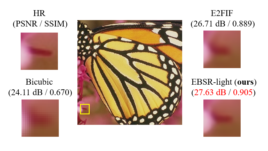
Figure 8: Qualitative comparison of our EBSR-light with the prior art network on a $\times 4$ super-resolution.

6.3 Memory and Computation Cost

We now evaluate the memory and computation cost of our proposed EBSR-light and EBSR. We compute the total operations and parameters following [31] and [15] as below:

$$OPs=FLOPs+BOPs/64$$ (7)

$$Params=Param_{fp}+Param_{bi}/32$$

where $BOPs$ and $Param_{bi}$ denote the number of binary operations and parameters. We choose a $128\times 128$ input image at $\times 4$ scale for evaluation. Compared with the FP SRResNet and EDSR, our EBSR-light and EBSR reduce memory usage by $38\times$ and $39\times$, respectively, and reduce computation by $29\times$ and $58\times$, respectively. The computation cost of our models is slightly larger than E2FIF in exchange for much higher performance as discussed above.

We notice that the spatial re-scaling module introduces many FP operations. This is because the convolution layer in Figure 5(a) outputs a feature map with $H\times W$ spatial dimension, which is usually large for SR. Thus we propose EBSR-SQ to quantize the spatial re-scaling module to low-bits. We quantize the weights and activations following [5] and calculated the equivalent operations and parameters of EBSR-SQ following [31]. We try three different configurations as shown in Table 4, all of which achieve better performance compared to the SRResNet-E2FIF with fewer operations. Specifically, EBSR-SQ with 4-bit weight and 4-bit activation improves the PSNR by 0.26 dB and 0.27dB on Set5 and Urban100, respectively, over SRResNet-E2FIF, with 0.01 G fewer operations.

6.4 Ablation Study

We conduct ablation studies based on our strong baseline model to analyze the individual effect of our methods. We also compare our methods with the per-channel activation quantization. As we have discussed in Section 3, per-channel activation quantization is not hardware friendly. Hence, we focus on the performance comparison with it.

As shown in Table 5, compared with the baseline model, the spatial re-scaling method has 0.24 dB and 0.22 dB improvement on Set5 and Urban100, respectively. While the improvements of the channel-wise shifting and re-scaling method are 0.07 dB and 0.03 dB on the two datasets. Our model EBSR-light out-performs the per-channel quantization by 0.26 dB and 0.24 dB on the two datasets while being much more hardware friendly. The reason that spatial re-scaling is more effective than channel-wise shifting and re-scaling is probably that in our strong baseline, we have already used RSign with learnable bias to binarize activations which alleviate the impact of channel-wise variation.

Table 6: Comparison of our proposed EBSR-light with other BNNs for image super-resolution. All the models in this table have a similar lightweight backbone, which has 16 blocks and 64 channels. Note that fp denotes the full-precision model.

Model	Scale	Set5		Set14		B100		Urban100
		PSNR	SSIM	PSNR	SSIM	PSNR	SSIM	PSNR	SSIM
SRResNet-fp	x2	37.76	0.958	33.27	0.914	31.95	0.895	31.28	0.919
Bicubic	x2	33.66	0.930	30.24	0.869	29.56	0.843	26.88	0.840
SRResNet-BNN	x2	35.21	0.942	31.55	0.896	30.64	0.876	28.01	0.869
SRResNet-DoReFa	x2	36.09	0.950	32.09	0.902	31.02	0.882	28.87	0.880
SRResNet-BAM	x2	37.21	0.956	32.74	0.910	31.60	0.891	30.20	0.906
SRResNet-E2FIF	x2	37.50	0.958	32.96	0.911	31.79	0.894	30.73	0.913
EBSR-light (ours)	x2	37.64	0.958	33.16	0.913	31.88	0.895	31.11	0.917
SRResNet-fp	x3	34.07	0.922	30.04	0.835	28.91	0.798	27.50	0.837
Bicubic	x3	30.39	0.868	27.55	0.774	27.21	0.739	24.46	0.735
SRResNet-BNN	x3	31.18	0.877	28.29	0.799	27.73	0.765	25.03	0.758
SRResNet-DoReFa	x3	32.44	0.903	28.99	0.811	28.21	0.778	25.84	0.783
SRResNet-BAM	x3	33.33	0.915	29.63	0.827	28.61	0.790	26.69	0.816
SRResNet-E2FIF	x3	33.65	0.920	29.67	0.830	28.72	0.795	27.01	0.825
EBSR-light (ours)	x3	33.89	0.921	29.95	0.834	28.82	0.797	27.33	0.833
SRResNet-fp	x4	31.76	0.888	28.25	0.773	27.38	0.727	25.54	0.767
Bicubic	x4	28.42	0.810	26.00	0.703	25.96	0.668	23.14	0.658
SRResNet-BNN	x4	29.33	0.826	26.72	0.728	26.45	0.692	23.68	0.683
SRResNet-DoReFa	x4	30.38	0.862	27.48	0.754	26.87	0.708	24.45	0.720
SRResNet-BAM	x4	31.24	0.878	27.97	0.765	27.15	0.719	24.95	0.745
SRResNet-E2FIF	x4	31.33	0.880	27.93	0.766	27.20	0.723	25.08	0.750
EBSR-light (ours)	x4	31.64	0.885	28.22	0.772	27.30	0.727	25.36	0.761

Table 7: Comparison of our proposed EBSR with other BNNs for image super-resolution. All the models in this table have 32 blocks and 256 channels. Note that fp here denotes the full-precision model.

Method	Scale	Set5		Set14		B100		Urban100
		PSNR	SSIM	PSNR	SSIM	PSNR	SSIM	PSNR	SSIM
EDSR-fp	x2	38.11	0.960	33.92	0.920	32.32	0.901	32.93	0.935
Bicubic	x2	33.66	0.930	30.24	0.869	29.56	0.843	26.88	0.840
EDSR-BNN	x2	34.47	0.938	31.06	0.891	30.27	0.872	27.72	0.864
EDSR-BiReal	x2	37.13	0.956	32.73	0.909	31.54	0.891	29.94	0.903
EDSR-IBTM	x2	37.80	0.960	33.38	0.916	32.04	0.898	31.49	0.922
EDSR-E2FIF	x2	37.95	0.960	33.37	0.915	32.13	0.899	31.79	0.924
EBSR (ours)	x2	37.99	0.959	33.52	0.916	32.10	0.898	31.96	0.926
EDSR-fp	x3	34.65	0.928	32.52	0.846	29.25	0.809	28.80	0.865
Bicubic	x3	30.39	0.868	27.55	0.774	27.21	0.739	24.46	0.735
EDSR-BNN	x3	20.85	0.399	19.47	0.299	19.23	0.285	18.18	0.307
EDSR-BiReal	x3	33.17	0.914	29.53	0.826	28.53	0.790	26.46	0.801
EDSR-IBTM	x3	34.10	0.924	30.11	0.838	28.93	0.801	27.49	0.839
EDSR-E2FIF	x3	34.24	0.925	30.06	0.837	29.00	0.802	27.84	0.844
EBSR (ours)	x3	34.36	0.925	30.28	0.840	29.04	0.803	28.06	0.849
EDSR-fp	x4	32.46	0.897	28.80	0.787	27.71	0.742	26.64	0.803
Bicubic	x4	28.42	0.810	26.00	0.703	25.96	0.668	23.14	0.658
EDSR-BNN	x4	17.53	0.188	17.51	0.160	17.15	0.151	16.35	0.163
EDSR-BiReal	x4	30.81	0.871	27.71	0.760	27.01	0.716	24.66	0.733
EDSR-IBTM	x4	31.84	0.890	28.33	0.777	27.42	0.732	25.54	0.769
EDSR-E2FIF	x4	31.91	0.890	28.29	0.755	27.44	0.731	25.74	0.774
EBSR (ours)	x4	32.20	0.892	28.56	0.780	27.54	0.735	26.06	0.783

7 Conclusion

In this work, we observe the large pixel-to-pixel, channel-to-channel, and image-to-image variations in FP SR networks, which contain important detailed information for SR. To preserve these information in BNNs, we first construct a strong baseline utilizing robust binarization methods and propose the spatial re-scaling as well as channel-wise shifting and re-scaling methods. Then we construct EBSR, EBSR-light, and EBSR-SQ. Compared to the prior art, the proposed models capture more detailed information for SR and significantly bridge the performance gap between BNN and FP SR networks in low computation and memory costs. Specifically, EBSR-light improves the PSNR by 0.31 dB and 0.28 dB compared to SRResNet-E2FIF while EBSR outperforms EDSR-E2FIF by 0.29 dB and 0.32 dB PSNR for $\times 4$ SR on Set5 and Urban100 respectively.

Appendix A Appendix

In this appendix, we provide more qualitative evaluation results of our proposed EBSR-light and EBSR-SQ below in Figure 9. It can be seen that compared with the prior art model, our proposed models reconstruct better-looking SR images. They are more clear and more realistic in some detailed textures. It is noticeable that our EBSR-SQ (W4A4) with 0.01G fewer operations than E2FIF exhibits better visual perception as well.

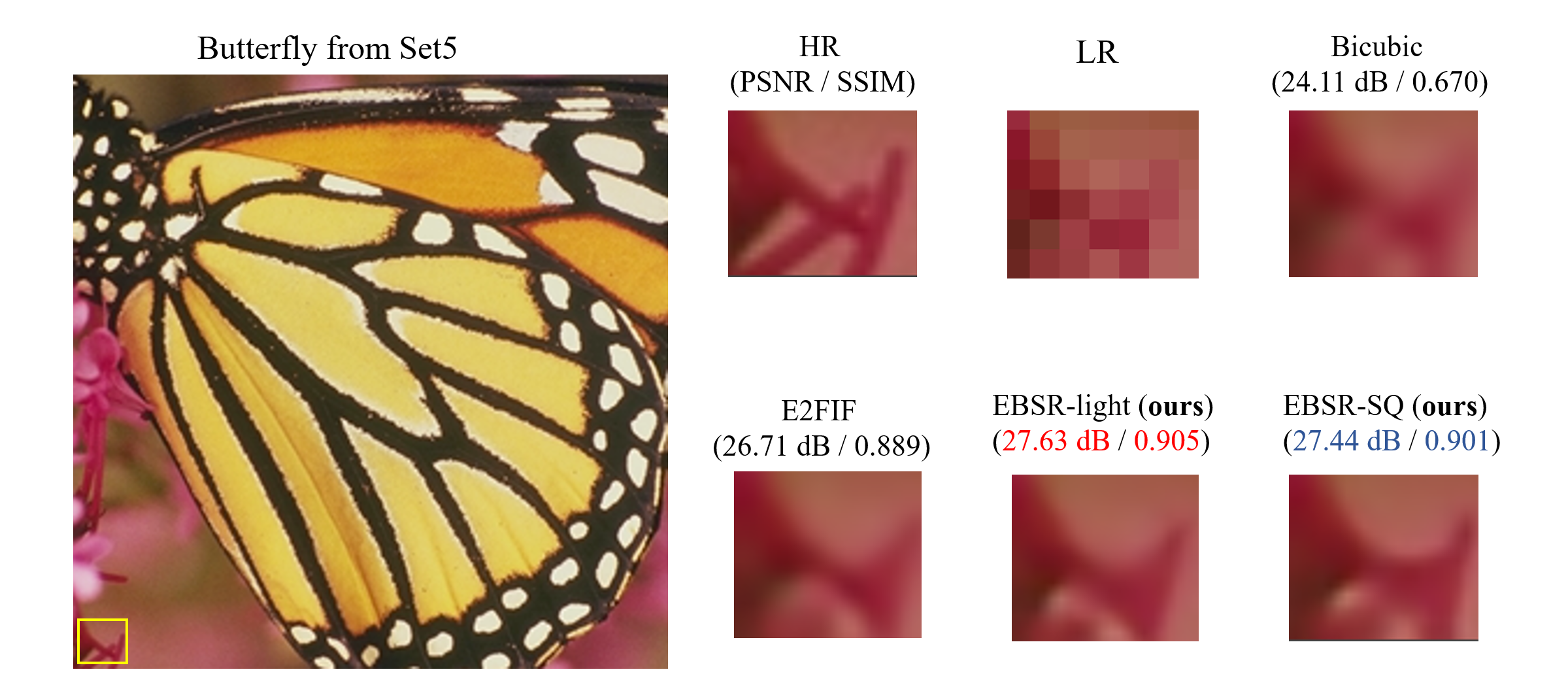
((a))

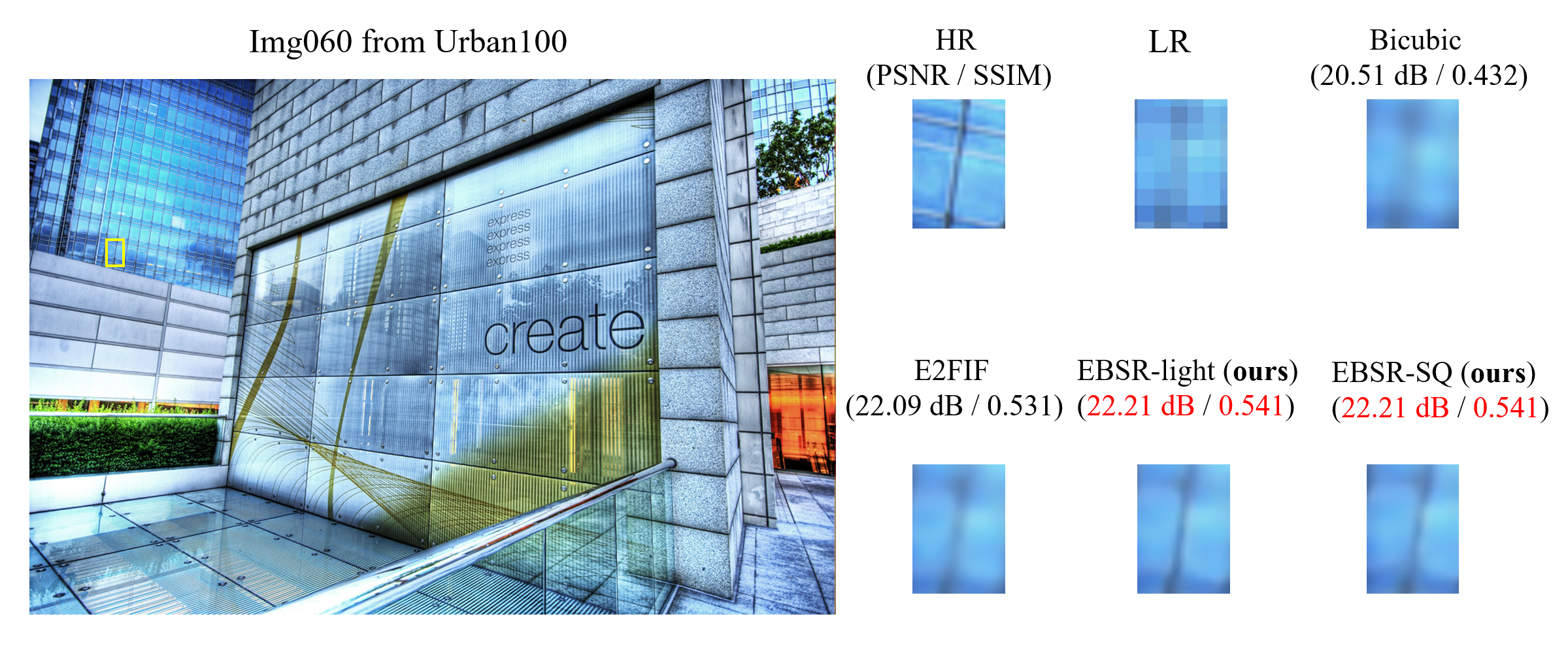
((b))

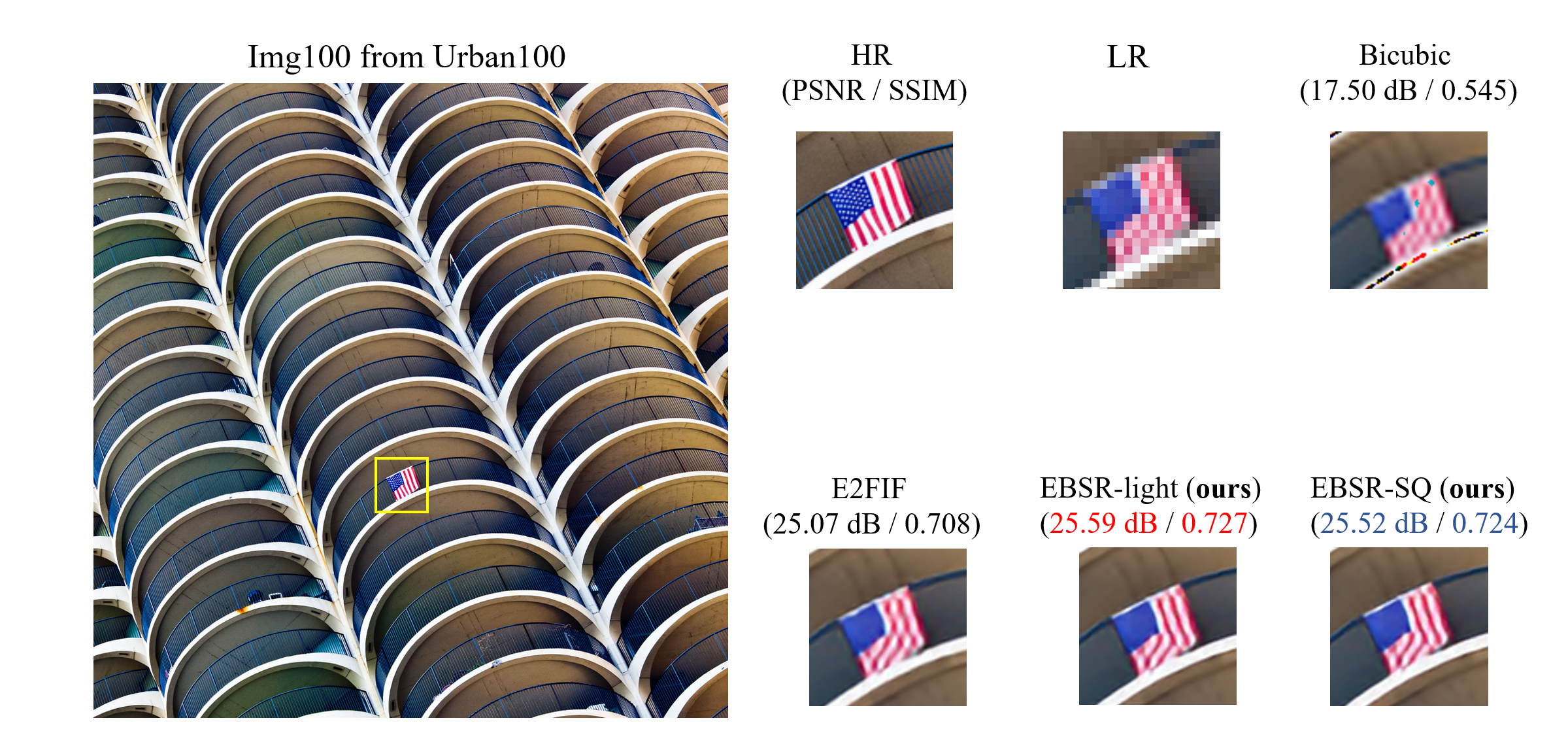
((c))

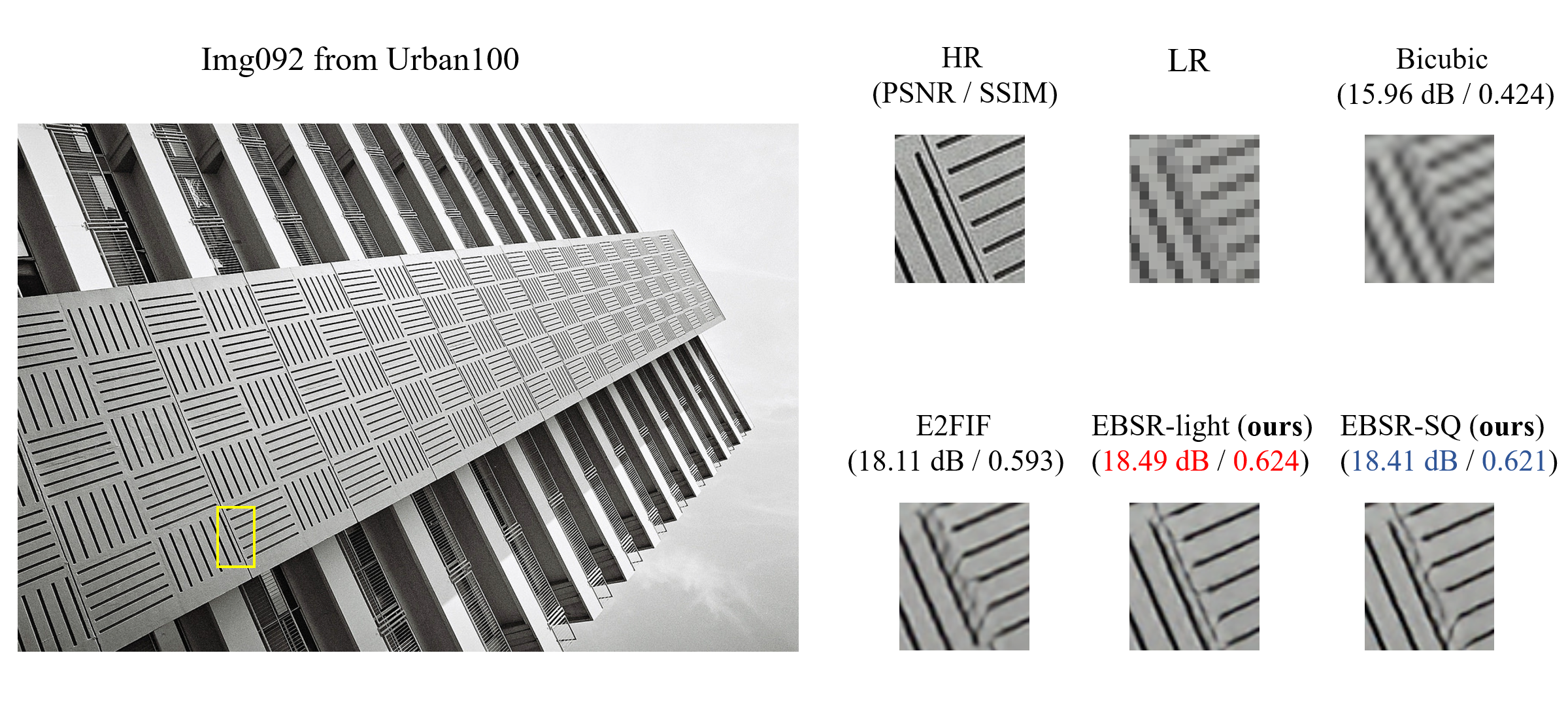
((d))

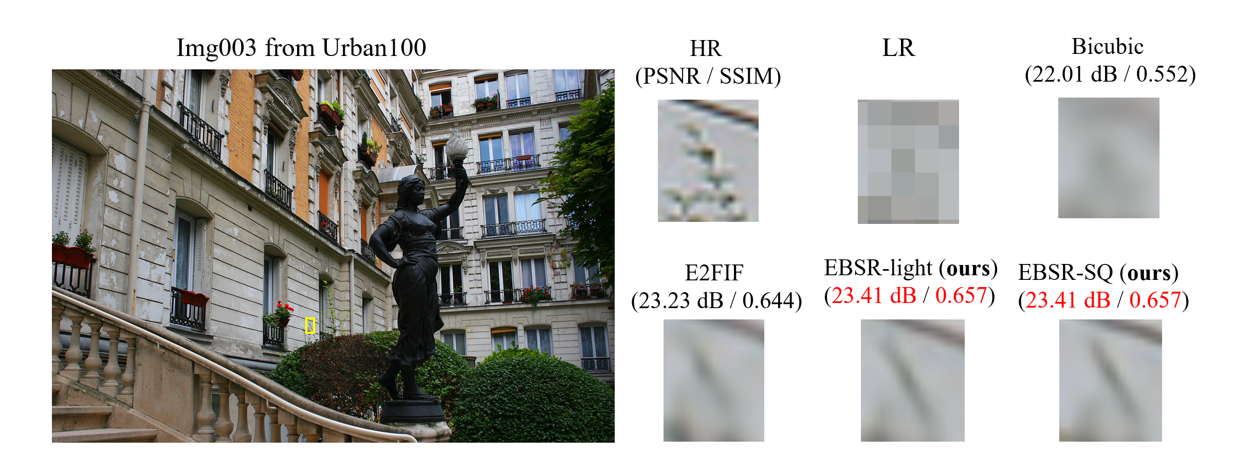
((e))

Figure 9: Qualitative comparison of our models with others on $\times 4$ super-resolution. Red indicates the best performance and blue indicates the second best.

References

- [1] Haoli Bai, Wei Zhang, Lu Hou, Lifeng Shang, Jing Jin, Xin Jiang, Qun Liu, Michael Lyu, and Irwin King. Binarybert: Pushing the limit of bert quantization. arXiv preprint arXiv:2012.15701, 2020.
- [2] Marco Bevilacqua, Aline Roumy, Christine Guillemot, and Marie Line Alberi-Morel. Low-complexity single-image super-resolution based on nonnegative neighbor embedding. 2012.
- [3] Adrian Bulat and Georgios Tzimiropoulos. Xnor-net++: Improved binary neural networks. arXiv preprint arXiv:1909.13863, 2019.
- [4] Chao Dong, Chen Change Loy, Kaiming He, and Xiaoou Tang. Image super-resolution using deep convolutional networks. IEEE transactions on pattern analysis and machine intelligence, 38(2):295–307, 2015.
- [5] Steven K Esser, Jeffrey L McKinstry, Deepika Bablani, Rathinakumar Appuswamy, and Dharmendra S Modha. Learned step size quantization. arXiv preprint arXiv:1902.08153, 2019.
- [6] Cheeun Hong, Heewon Kim, Sungyong Baik, Junghun Oh, and Kyoung Mu Lee. Daq: Channel-wise distribution-aware quantization for deep image super-resolution networks. In Proceedings of the IEEE/CVF Winter Conference on Applications of Computer Vision, pages 2675–2684, 2022.
- [7] Jia-Bin Huang, Abhishek Singh, and Narendra Ahuja. Single image super-resolution from transformed self-exemplars. In Proceedings of the IEEE conference on computer vision and pattern recognition, pages 5197–5206, 2015.
- [8] Xinrui Jiang, Nannan Wang, Jingwei Xin, Keyu Li, Xi Yang, and Xinbo Gao. Training binary neural network without batch normalization for image super-resolution. In Proceedings of the AAAI Conference on Artificial Intelligence, volume 35, pages 1700–1707, 2021.
- [9] Jiwon Kim, Jung Kwon Lee, and Kyoung Mu Lee. Accurate image super-resolution using very deep convolutional networks. In Proceedings of the IEEE conference on computer vision and pattern recognition, pages 1646–1654, 2016.
- [10] Zhiqiang Lang, Lei Zhang, and Wei Wei. E2fif: Push the limit of binarized deep imagery super-resolution using end-to-end full-precision information flow. arXiv preprint arXiv:2207.06893, 2022.
- [11] Christian Ledig, Lucas Theis, Ferenc Huszár, Jose Caballero, Andrew Cunningham, Alejandro Acosta, Andrew Aitken, Alykhan Tejani, Johannes Totz, Zehan Wang, et al. Photo-realistic single image super-resolution using a generative adversarial network. In Proceedings of the IEEE conference on computer vision and pattern recognition, pages 4681–4690, 2017.
- [12] Huixia Li, Chenqian Yan, Shaohui Lin, Xiawu Zheng, Baochang Zhang, Fan Yang, and Rongrong Ji. Pams: Quantized super-resolution via parameterized max scale. In Computer Vision–ECCV 2020: 16th European Conference, Glasgow, UK, August 23–28, 2020, Proceedings, Part XXV 16, pages 564–580. Springer, 2020.
- [13] Bee Lim, Sanghyun Son, Heewon Kim, Seungjun Nah, and Kyoung Mu Lee. Enhanced deep residual networks for single image super-resolution. In Proceedings of the IEEE conference on computer vision and pattern recognition workshops, pages 136–144, 2017.
- [14] Zechun Liu, Zhiqiang Shen, Marios Savvides, and Kwang-Ting Cheng. Reactnet: Towards precise binary neural network with generalized activation functions. In Computer Vision–ECCV 2020: 16th European Conference, Glasgow, UK, August 23–28, 2020, Proceedings, Part XIV 16, pages 143–159. Springer, 2020.
- [15] Zechun Liu, Baoyuan Wu, Wenhan Luo, Xin Yang, Wei Liu, and Kwang-Ting Cheng. Bi-real net: Enhancing the performance of 1-bit cnns with improved representational capability and advanced training algorithm. In Proceedings of the European conference on computer vision (ECCV), pages 722–737, 2018.
- [16] Yinglan Ma, Hongyu Xiong, Zhe Hu, and Lizhuang Ma. Efficient super resolution using binarized neural network. In Proceedings of the IEEE/CVF Conference on Computer Vision and Pattern Recognition Workshops, pages 0–0, 2019.
- [17] David Martin, Charless Fowlkes, Doron Tal, and Jitendra Malik. A database of human segmented natural images and its application to evaluating segmentation algorithms and measuring ecological statistics. In Proceedings Eighth IEEE International Conference on Computer Vision. ICCV 2001, volume 2, pages 416–423. IEEE, 2001.
- [18] Brais Martinez, Jing Yang, Adrian Bulat, and Georgios Tzimiropoulos. Training binary neural networks with real-to-binary convolutions. arXiv preprint arXiv:2003.11535, 2020.
- [19] Markus Nagel, Marios Fournarakis, Rana Ali Amjad, Yelysei Bondarenko, Mart Van Baalen, and Tijmen Blankevoort. A white paper on neural network quantization. arXiv preprint arXiv:2106.08295, 2021.
- [20] Mohammad Rastegari, Vicente Ordonez, Joseph Redmon, and Ali Farhadi. Xnor-net: Imagenet classification using binary convolutional neural networks. In Computer Vision–ECCV 2016: 14th European Conference, Amsterdam, The Netherlands, October 11–14, 2016, Proceedings, Part IV, pages 525–542. Springer, 2016.
- [21] Mark Sandler, Andrew Howard, Menglong Zhu, Andrey Zhmoginov, and Liang-Chieh Chen. Mobilenetv2: Inverted residuals and linear bottlenecks. In Proceedings of the IEEE conference on computer vision and pattern recognition, pages 4510–4520, 2018.
- [22] Radu Timofte, Eirikur Agustsson, Luc Van Gool, Ming-Hsuan Yang, and Lei Zhang. Ntire 2017 challenge on single image super-resolution: Methods and results. In Proceedings of the IEEE conference on computer vision and pattern recognition workshops, pages 114–125, 2017.
- [23] Zhou Wang, Alan C Bovik, Hamid R Sheikh, and Eero P Simoncelli. Image quality assessment: from error visibility to structural similarity. IEEE transactions on image processing, 13(4):600–612, 2004.
- [24] Zhihao Wang, Jian Chen, and Steven CH Hoi. Deep learning for image super-resolution: A survey. IEEE transactions on pattern analysis and machine intelligence, 43(10):3365–3387, 2020.
- [25] Jingwei Xin, Nannan Wang, Xinrui Jiang, Jie Li, Heng Huang, and Xinbo Gao. Binarized neural network for single image super resolution. In Computer Vision–ECCV 2020: 16th European Conference, Glasgow, UK, August 23–28, 2020, Proceedings, Part IV 16, pages 91–107. Springer, 2020.
- [26] Roman Zeyde, Michael Elad, and Matan Protter. On single image scale-up using sparse-representations. In Curves and Surfaces: 7th International Conference, Avignon, France, June 24-30, 2010, Revised Selected Papers 7, pages 711–730. Springer, 2012.
- [27] Yulun Zhang, Kunpeng Li, Kai Li, Lichen Wang, Bineng Zhong, and Yun Fu. Image super-resolution using very deep residual channel attention networks. In Proceedings of the European conference on computer vision (ECCV), pages 286–301, 2018.
- [28] Yulun Zhang, Kunpeng Li, Kai Li, Bineng Zhong, and Yun Fu. Residual non-local attention networks for image restoration. arXiv preprint arXiv:1903.10082, 2019.
- [29] Yulun Zhang, Yapeng Tian, Yu Kong, Bineng Zhong, and Yun Fu. Residual dense network for image super-resolution. In Proceedings of the IEEE conference on computer vision and pattern recognition, pages 2472–2481, 2018.
- [30] Yunshan Zhong, Mingbao Lin, Xunchao Li, Ke Li, Yunhang Shen, Fei Chao, Yongjian Wu, and Rongrong Ji. Dynamic dual trainable bounds for ultra-low precision super-resolution networks. In Computer Vision–ECCV 2022: 17th European Conference, Tel Aviv, Israel, October 23–27, 2022, Proceedings, Part XVIII, pages 1–18. Springer, 2022.
- [31] Shuchang Zhou, Yuxin Wu, Zekun Ni, Xinyu Zhou, He Wen, and Yuheng Zou. Dorefa-net: Training low bitwidth convolutional neural networks with low bitwidth gradients. arXiv preprint arXiv:1606.06160, 2016.