Community detection in complex networks via node similarity, graph representation learning, and hierarchical clustering

Abstract

Community detection is a critical challenge in analysing real graphs, including social, transportation, citation, cybersecurity, and many other networks. This article proposes three new, general, hierarchical frameworks to deal with this task. The introduced approach supports various linkage-based clustering algorithms, vertex proximity matrices, and graph representation learning models. We compare over a hundred module combinations on the Stochastic Block Model graphs and real-life datasets. We observe that our best pipelines (Wasserman–Faust and the mutual information-based PPMI proximity, as well as the deep learning-based DNGR representations) perform competitively to the state-of-the-art Leiden and Louvain algorithms. At the same time, unlike the latter, they remain hierarchical. Thus, they output a series of nested partitions of all possible cardinalities which are compatible with each other. This feature is crucial when the number of correct partitions is unknown in advance.

1 Introduction

1.1 Background

More and more structures become available in the form of graphs and networks. The problem of community detection therein is a long-standing task in data science: a plethora of solutions have already been developed (see, e.g., [23, 57, 63, 35]). Still, the topic seems far from exhausted [24, 56]. What constitutes a community can be understood very broadly [23]. Therefore, many relatively different tools will aim to provide us with their own solutions to this task: is a community a group of tightly connected vertices, or is it a group of vertices that play similar roles in the graph’s structure? Further, the sole existence of some mathematically definable relation allows us to construct a network in a given environment. However, such networks may be, for example, structured, hierarchical, temporal, evolving, or attributed. The various generalisations of the concept of a graph call for different community detection solutions tailored to each specific context [23, 14, 21].

Researchers in pattern recognition and statistical/machine learning have long known a similar problem under a different name: clustering [64]. At some level, we can say that the only difference between clustering and community detection is the data space considered – the former is defined on graphs and the latter on other metric spaces, such as the Euclidean one [64]. This similarity resulted in some domain-specific approaches stemming from a common theoretical basis. For example, hierarchical algorithms may be successfully employed to solve both community detection and clustering tasks with little change in the implementation. However, with the need of more specialised methods [57], the approaches developed in the two aforementioned fields began to diverge.

1.2 Research objectives

Taking into account the growing popularity of graph machine learning (e.g., [34, 52, 40]), which includes graph representation learning specifically, we wish to help bridge the between-domain gap by exploring new ways of connecting community detection and clustering solutions.

Specifically, in this paper, we develop a framework for applying hierarchical clustering algorithms (e.g., [45, 27, 67]) to the task of community detection. While perhaps not the newest by itself, the hierarchical approach turns out robust and easily applicable on graphs because it relies solely on similarity metrics between the pairs of nodes. As the problem of choosing the right measures for our task is crucial, we will perform an extensive comparative analysis of twenty five vertex similarity modelling techniques falling into the three following classes:

1. distance matrices obtained by considering various node similarity measure: the Wasserman–Faust measure [62], Neighbourhood overlap [23], $K$-step walk probability [23], Katz index [38], Rooted PageRank [48], Adamic–Adar index [1], Blondel–Gajardo measure [4], and Positive Pointwise Mutual Information [11],

2. spectral versions of the above, i.e., eigendecompositions of the corresponding vertex similarity matrices,

3. distances on automatically discovered spaces using the representation learning algorithms: DeepWalk [52], DNGR [11], Graph Factorisation [2], GraRep [10], HARP [13], HOPE [48], Laplacian Eigenmaps [3], and Node2Vec [32].

Both synthetic and real-life network examples will be used. Further, we shall study how the tuning of the underlying parameters affects the quality of clustering. In each case, we will determine the best linkage function. This will also provide us with a good opportunity to consider a new graph extension of the recently-proposed Genie algorithm [27], whose performance on many benchmark datasets in the Euclidean spaces turned out to be above par [25].

We should emphasise that hierarchical approaches come with a set of advantages. Firstly, the communities are nested, i.e., depending on the selected number of clusters we can observe how a large community can be decomposed into smaller ones. Also, hierarchical approaches allow us to select any number of clusters, which is a feature often lacking in other methods.

The paper is set out as follows. In Section 2, we introduce the node similarity measures and graph representation learning methods that will serve as graph models in the task at hand. In Section 3, we present a framework for community detection based on hierarchical clustering algorithms (including Genie). In Section 4, we evaluate all the algorithms on synthetic datasets from the stochastic block model in order to determine the best method combinations. They are then carefully evaluated, including on real-world data, in Section 5. Finally, Section 6 concludes the article.

2 Graph models

In this section, we present selected vertex similarity measures we investigate in our framework.

2.1 Community detection

A common way of conducting mathematical research is to find generalisations of the existing concepts to explain them better in connection with the definitions from other fields. In that sense, Network Science is not that different: why should we define a “small” graph, such as a citation network of machine learning papers, when we could define a more general citation network of all academic research? This approach allows us to work on larger structures, which usually means that we obtain better statistical approximations of some sought values. Nevertheless this also inevitably indicates that our network becomes less homogeneous. In fact, while the whole citation network contains all the domains, we should expect that its subgraph induced by the vertices representing ML should be connected more densely than the whole network on average. Such an induced subgraph is called a community [23]. In general, communities can be found in many naturally occurring networks, e.g., they may be based on shared interests of social media users in a social network [33, 9], finding patterns in delays in railway networks [18], or similarity between protein functions in biological networks [29].

Therefore, to understand the behaviour of a network correctly, it is essential to detect whether it contains communities and, if so, find which nodes belong to which clusters. However, the above description of a community is far from strict. In fact, there is no universally accepted definition [23, 24]. Here we would like to present some metrics that could help define the community.

Definition 1.

Let $H=(V_{H},E_{H})$ be an induced subgraph of graph $G=(V_{G},E_{G})$ and let $n_{H}=|V_{H}|$. We say that $e$ is an internal edge of $H$, if it connects two vertices in $V_{H}$. Also, $e$ is an inter-cluster edge of $H$, if exactly one of its ends lies in $V_{H}$. As the maximum number of edges in $H$ is equal to $\binom{n_{H}}{2}=\frac{n_{H}(n_{H}-1)}{2}$, we define the intra- and inter-cluster densities of $H$, respectively, as [23]:

$$\delta_{\text{int}}(H) = \frac{\text{the number of internal edges of $H$}}{\binom{n_{H}}{2}},$$ (1)

$$\delta_{\text{ext}}(H) = \frac{\text{the number of inter-cluster edges of $H$}}{n_{H}(n-n_{H})}.$$ (2)

Intuitively, a community, regarded as an induced subgraph of $G$, should have higher inter-cluster density and lower intra-cluster density than the average link density of the graph $G$. To detect communities, we could look for a partition that either maximises the average value of $\delta_{\text{int}}$, minimises the average value of $\delta_{\text{ext}}$, or combines the two; for example, we could maximise the average value of $\delta_{\text{int}}-\delta_{\text{ext}}$ [43]. However, the problem with algorithms simply relying on the above-defined concepts of cluster density is that the posed tasks are often NP-complete. For example, finding all clusters in $G$ that have intra-cluster density $\delta_{\text{int}}$ higher than a given threshold $\zeta$ cannot be performed in polynomial time [28].

Another issue with the above definitions of cluster density is that we calculate them only relative to the observed network $G$. If $G$ is heterogeneous, it becomes difficult to precisely define the requirements for a subgraph to be a community. For example, we would require a community to have an extremely high density if it lies in a densely connected region of $G$, but we would accept a subgraph with a lower density in a sparse region in $G$. Such differences could lead to problems with proper task definition and unreliable results. On the other hand, we know that the Erdős–Rényi (ER) model [20] should not contain communities, as the edges are positioned randomly with equal probabilities. Based on that fact, Newman and Girvan introduced a concept of modularity [46].

Definition 2.

Let $G=(V,E)$ and let us assume that we have partitioned $G$ into clusters and let $A$ be its adjacency matrix. Let $\tilde{G}$ be a null model, i.e., a graph that is structurally similar to $G$ but does not contain communities. Let $\tilde{A}_{i,j}$ be the expected number of edges between $i,j$ in $\tilde{G}$ and let $C_{i}$ denote the cluster in $G$ containing the vertex $i$. Then, denoting the Kronecker delta with $\delta$, we define a partition quality function called modularity as:

$$Q=\frac{1}{2|E|}\sum_{i,j\in V}(A_{i,j}-P_{i,j})\,\delta(C_{i},C_{j}).$$ (3)

Intuitively, given some partition of $G$, modularity compares the observed number of edges in the communities with the expected number of such edges in the null model. Various candidates for the null model have been investigated: the ER model is the simplest of them all [46], but we could derive specific null models for particular classes of networks [51]. While explicitly maximising modularity is again NP-complete, it has become a popular evaluation metric for community detection algorithms [23].

2.2 Node similarity

In the previous section, we have defined the community to be an induced subgraph, which is, in some sense, connected more strongly than its neighbourhood. However, we could look at the community detection problem more locally: a community could be a subgraph of somewhat similar vertices. In such an approach, we would like the communities to be subgraphs such that the inter-cluster edges connect similar vertices and the intra-cluster edges connect different ones [23]. Assuming that two vertices are similar if they are connected in the graph, we naturally return to the previous definition. However, the flexibility of similarity allows us to introduce other approaches to community detection. In this section, we will present some selected node similarity measures.

Embedding-based measures [23].

Let us assume that we have embedded the graph $G$ in the space $\mathbb{R}^{d}$ for some $d$, i.e., that we have vector representations $X_{v}=(x^{1}_{v},x^{2}_{v},\dots,x^{d}_{v})\in\mathbb{R}^{d}$ for each node $v$ of $G$. Regardless of how the embedding was obtained, we can now easily define the node similarity between two vertices $u$ and $v$ as a distance between $X_{u}$ and $X_{v}$, e.g., being the Euclidean, Manhattan, and Chebyshev metric. Applying any non-increasing transformation thereon turns them into a similarity function. We will discuss particular graph embedding methods in Section 2.3.

Relationship-based measures [23, 8].

Another class of similarity measures is based on the relationships encoded within the graph. The most straightforward function of the similarity between the vertices $u$ and $v$ of $G$ is $A_{u,v}$, i.e., the element of the graph’s adjacency matrix indicating whether or not $u$ and $v$ are adjacent. However, we could also define their similarity in terms of the structure of their neighbourhoods, e.g., based on the Wasserman–Faust distance [62]:

$$d^{WF}_{u,v}=\sqrt{\sum_{k\neq u,v}(A_{u,k}-A_{v,k})^{2}}.$$ (4)

The Wasserman–Faust distance is one of the first measures based on the structural equivalence of the vertices. It does not rely on the adjacency of $u$ and $v$. The Adamic–Adar index [1] also incorporates the structural equivalence:

$$d^{AA}_{u,v}=\sum_{w\in N(u)\cap N(v)}\frac{2}{\log|N(w)|}.$$ (5)

The intuition behind this index is that the common neighbours having large neighbourhoods are less significant to the similarity between the vertices. Another variant of the similarity measure based on neighbourhoods of $u$ and $v$ is the Jaccard (Overlap), similarity:

$$w_{u,v}=\frac{|N_{G}(u)\cap N_{G}(v)|}{|N_{G}(u)\cup N_{G}(v)|}.$$ (6)

Walk-based measures.

In another approach, we could measure similarity between the vertices based on walks in the graph. Intuitively, if many paths connect two vertices, they would seem similar. Fortunately, the adjacency matrix of a graph captures all information about paths. It is known that for an unweighted graph $G$, the element $A_{u,v}^{k}$ counts the number of paths between the vertices $u,v$ of length exactly $k$ [30]. For instance, the Katz index matrix [38] is:

$$S^{\text{Katz}}=\sum_{l=1}^{\infty}\beta A^{l}=\beta\cdot(I-\beta\cdot A)^{-1}\cdot A,$$ (7)

where $\beta$ is a decay parameter, and $I$ denotes the identity matrix. Then, the value $S^{\text{Katz}}_{u,v}$ gives the walk-based similarity between the vertices $u$ and $v$.

We may also be interested in whether the two vertices $u$ and $v$ often co-occur in the graph’s random walks. This approach differs slightly from the previous one, as it assumes that the co-occurrence in random walks gives more practical information about the similarity between the two vertices than the Katz index. If $D$ is the degree matrix of $G$, then the $K$-step transition probability between the vertices $u$ and $v$ may be retrieved cia [53]:

$$d^{K}_{i,j}=((D^{-1}A)^{K})_{i,j}.$$ (8)

Similarly, instead of using unbiased random walks, we could turn to more sophisticated tools like the Rooted PageRank algorithm [49, 48]. It assumes that we “surf” through the vertices and walk to some neighbour with probability $\alpha$, or return to the starting vertex with the probability $1-\alpha$. If $P$ is the transition probability matrix, we get that $S^{\text{RPR}}=\alpha\cdot S^{\text{RPR}}\cdot P+(1-\alpha)\cdot I$, which can be solved to obtain:

$$S^{\text{RPR}}=(1-\alpha)(I-\alpha P)^{-1}.$$ (9)

The elements of this matrix correspond to node similarity based on the Rooted PageRank algorithm.

Finally, we can use random walks to estimate the value of Pointwise Mutual Information (PMI) [15] between the vertices. That is, we identify the similarity between $u$ and $v$ as:

$$\text{PMI}(u,v)=\log\frac{p(u,v)}{p(u)p(v)},$$ (10)

where $p(u)$ denotes the probability of the occurrence of $u$ in some random walk of a fixed length. Analogically, $p(u,v)$ denotes the probability that both vertices occur on the same random walk, calculated using powers of a transition matrix of a stochastic random walk on the graph. Usually, as the PMI values may be negative, we use the Positive Pointwise Mutual Information (PPMI), i.e., we replace all the negative elements with $0$; see [11] for an example use.

2.3 Graph representation learning

We will use several algorithms which can be loosely divided into five categories: direct optimisation-based, matrix factorisation-based, random walk-based, and autoencoder-based methods capturing vertex proximity, and a separate class of algorithms capturing structural similarity of vertices. Let us present a short description of each of the categories and their noteworthy instances. For the sake of clarity, throughout this section, we assume that we embed the nodes of a graph $G=(V,E)$ in $\mathbb{R}^{d}$, i.e., we obtain a matrix $Z\in\mathbb{R}^{|V|\times d}$ whose rows correspond to individual nodes. We also denote the adjacency matrix of $G$ with $A$, its Laplacian with $L$, and its degree matrix with $D$.

Direct optimisation methods.

This class of methods generates the embedding of $G$ by solving a specific optimisation task. For example, in the Laplacian Eigenmaps [3] algorithm, we select $Z$ which minimises $\operatorname{tr}(Z^{T}LZ)$ subject to $Z^{T}DZ=I$, where $\operatorname{tr}$ is the trace of a matrix. The authors of [3] justify that this optimisation task corresponds to a representation where adjacent nodes are possibly close in the resulting space while the non-adjacent nodes lie far from each other. Furthermore, in the Graph Factorisation (GF) [2] method, the similarity between the nodes $v_{i}$ and $v_{j}$ is approximated by the dot product of the corresponding representations, i.e., $s(v_{i},v_{j})\approx\langle Z_{i},Z_{j}\rangle.$

Matrix factorisation methods.

The second class of methods uses the Singular Value Decomposition (SVD), which creates a lower-dimensional approximation of higher-dimensional structures [31]. To obtain the embedding, we utilise the SVD on a matrix representation of a graph and again rely on the dot product $\langle Z_{i},Z_{j}\rangle$ approximation of the similarity. However, neither of the two methods performs the SVD on the adjacency or the Laplacian matrix as, according to the authors, these matrices are incapable of accurately representing node similarity. Thus, GraRep [10] performs the decomposition on a $K$-step transition probability matrix, and HOPE [48] allows the use of the aforementioned Katz Index, Adamic–Adar, Rooted PageRank, or Jaccard similarity matrices. It must be noted that HOPE is a tool developed specifically for directed graphs with asymmetric similarity matrices. We also should mention separately some SVD-based clustering algorithms, e.g., Lingo [47], which could be applied to graph matrices to directly perform community detection.

Random walk methods.

The next group of algorithms train an embedding model based on random walks in the graph. They all use the Skip-Gram model [44], which is a tool developed for Natural Language Processing. This design decision can be justified by the similarity of node sequences in a random walk and the word sequences in a sentence. Here, DeepWalk [52] is the most basic but efficient solution, in which first-order Markov walks in a graph are fed to the neural network to generate the embedding. Node2Vec [32] was developed to improve DeepWalk by replacing the walks with biased second-order Markov walks. Let us note that the authors of HARP [13] noticed inefficient weight propagation in the SkipGrap [44] neural network for large graphs. Therefore, they developed a meta-algorithm where the Skip-Gram model is trained iteratively on a family of graphs of increasing sizes derived from $G$. The weights corresponding to the nodes are passed between the iterations, improving the final representation. The HARP algorithm may work with either DeepWalk or Node2Vec as the underlying model.

Autoencoder methods.

These methods use an autoencoder neural network to generate an embedding. Specifically, a matrix representation of the graph $G$ is passed as input to both the neural network and the loss calculation. In that sense, autoencoder methods use a unary encoder in the described encoder-decoder architecture. Then, after the network is trained, the matrix $Z$ is retrieved from the middle of the autoencoder network. The two methods: SDNE [61] and DNGR [11], besides slight architecture changes, differ primarily in the input matrix representation. SDNE uses the graph adjacency matrix $A$, and DNGR uses the Positive Pointwise Mutual Information matrix.

Structural similarity methods.

In the previously described algorithms, each method aimed to capture the node similarity derived from the distance of the nodes in the graph. In contrast, the solutions belonging to the current class aim to capture some structural similarity, i.e., the similarity of the neighbourhoods of the vertices. Struc2Vec [55] generates a multigraph capturing the structural similarity of the nodes and then trains a Skip-Gram network to generate representations similarly to Node2Vec. GraphWave [19] uses graph signal processing methods on the graph Laplacian and converts the signals to random distributions of energy transferred between nodes.

2.4 Representation learning for community detection

As the primary goal of our work is to develop a general framework for community detection, we have reviewed recent works that use representation learning tools to solve the task at hand. However, as the domain is relatively young, very few representation learning-based algorithms have been introduced so far [37]. Below we present the most notable and representative ones.

vGraph: A generative model for joint community detection and node representation learning [58].

The presented solution – vGraph – is not precisely a representation-based community detection tool but a unified framework performing both community detection and node embedding. The authors heavily rely on node proximity theory derived for LINE [59] and introduce changes that account for better community detection. We assume that the network may be described with two prior probability distributions:

• $p(z|w)$, which represents the community distribution, $z$, for a given node $w$,

• $p(c|z)$, which represents the node distribution, $c$, for a given community $z$.

Given the above distributions, the authors describe a generative process of the network as drawing edges based on the social context of the neighbours. That is, an edge $(w,c)$ is generated with the probability:

$$p(c|w)=\sum_{z}p(c|z)p(z|w).$$ (11)

Given the above, we may estimate the probabilities over the network to detect communities. The probabilities for each node and community are parametrised with Euclidean representations of the nodes, which connects both tasks. A neural network is then trained to fit the probabilities to the observed network, resulting in both community detection and Euclidean node representations.

According to the authors’ results, vGraph can achieve competitive results in terms of modularity maximisation and state-of-the-art performance when used with supervised learning models for node classification. However, a possible drawback of the solution is that it allows for overlaps between communities, rendering it unsuitable for some use-cases.

Community detection based on graph representation learning in evolutionary networks [12].

LCDEN aims to generate Euclidean node representations of temporal networks, i.e., whose structure changes over time. This trait prohibits us from using standard “static” community detection tools as the communities change with the graph’s evolution. Its authors incorporate the same loss as the Laplacian Eigenmaps method to account for node information. However, to deal with the network evolution effectively, we assume time slices $t$ and the loss function given as:

$$L_{1}=2\operatorname{tr}\Big{(}Z_{t}^{T}L_{t-1}Z_{t}\Big{)}.$$ (12)

The authors use a deep sparse autoencoder network instead of performing a direct optimisation. This approach is motivated by the fact that sparse autoencoders may be less vulnerable to overfitting and still achieve satisfactory results for sparse networks due to the smaller volume of the overall structural information. To train the network, the authors employ an SE-based loss function with sparsely constrained parameters:

$$L_{2}=\sum\|(x_{i}^{\prime}-x_{i})\cdot(x_{i}(\beta-1)+1)\|_{2}^{2},$$ (13)

where $x_{i}^{\prime}$ and $x_{i}$ are the input and output representations of the node $i$, respectively, and $\beta$ is a tunable parameter. The loss function is then given as $L_{min}=\theta L_{1}+\gamma L_{2}$, where $\theta$ and $\gamma$ are some regularisation parameters.

Structural deep clustering network [6].

Structural Deep Clustering Network (SDCN) is a solution incorporating selected state-of-the-art deep learning frameworks for graph community detection. The primary motivation of the authors was based on two observations: that the autoencoder models tend to capture the possible community structure successfully and that Graph Convolutional Networks [40] outperform many other solutions in graph-related machine learning tasks. Therefore, the authors’ idea is to combine the two components into one large solution for community detection. To achieve that, they train a Deep Neural Network Autoencoder (DNN) on the consecutive layers of the GCN. To ensure the coherence of the components, a Dual Self-Supervised Module is introduced, which guides the training of the networks. Finally, the $K$-means clustering is performed on the resulting Euclidean for direct community detection. SDCN is currently one of the leading solutions for community detection in large networks, significantly outperforming other solutions, e.g., Variational Graph Autoencoders [39].

We refer the reader to the recent survey [57] for descriptions of other recent solutions, including deep learning models.

3 Distance-based graph clustering framework

3.1 Hierarchical clustering

Most hierarchical clustering methods are either divisive or agglomerative. DIANA [50] is an example of a divisive algorithm: starting from a single cluster $C_{1}$, we find the data point having maximal average dissimilarity to all the others and move it to a new cluster $C_{2}$. Then, all points that are now, on average, more similar to $C_{2}$ than $C_{1}$ are moved to $C_{2}$. The algorithm progresses iteratively until a predefined stopping requirement is met.

However, agglomerative algorithms are more popular due to better computational complexity and thus lie at the heart of our paper. Assuming a data set of points in a Euclidean space $S=\{s_{1},s_{2},\dots,s_{n}\}$, we first partition $S$ such that each point belongs to its own cluster, i.e., we define a partition consisting of singletons, $C=\{C_{1},C_{2},\dots,C_{n}\}$. Then, we merge clusters iteratively until a stop criterion is met: the desired number of clusters was reached. The merging strategy is what differentiates various algorithms. Denoting $d(s_{i},s_{j})$ as the selected distance measure from $s_{i}$ to $s_{j}$, we merge clusters $C_{m}$ and $C_{n}$ if they minimise a selected linkage criterion $D(C_{m},C_{n})$, with the single (minimum), complete (maximum), average, and Ward (variance) linkages being the most common choices; see, e.g., [45].

It must be noted that hierarchical clustering methods may also be based on graphs. For example, we could generate a graph using $k$-nearest neighbours methods and define a criterion using the degrees of nodes [66].

The single-linkage criterion is relatively naïve and often does not yield suitable partitions. The remaining ones have higher time complexity. One way to bypass the complexity problem is to add additional requirements. For example, the Genie algorithm [27, 25] uses a single-linkage criterion but simultaneously monitors the partition’s Gini index value, which a measure of inequality of cluster sizes. Only the cluster of the smallest cardinality can be merged when the algorithm reaches a predefined threshold of the Gini index value.

3.2 Proposed solution frameworks

We focus on the following three main sources from which we can obtain the communities: the node dissimilarity matrices, the eigenvectors of node similarity matrices, and the Euclidean representations of the nodes. As each of the above sources requires a slightly different approach to obtain the final community detection, we developed three frameworks which we detail below.

Algorithm 1 The proposed generic approaches to community detection via hierarchical clustering: a) node dissimilarity-based, b) spectral similarity-based, c) representation-based.

Input:
$G\text{ -- the input graph}$
$K\text{ -- the number of communities to detect}$
Output:
$C_{K}\text{ -- the partitioning of the nodes of the graph into}K\text{ communities}$
Algorithm:
a) $D\leftarrow\mathit{Dissimilarity}(G)$ b) $M\leftarrow\mathit{Similarity}(G)$ $Z\leftarrow\text{Matrix consisting of }K\\ \text{ eigenvectors of }M$ $D\leftarrow\text{Matrix of pairwise distances}\\ \text{(Euclidean) between all rows in }Z$ c) $Z\leftarrow\mathit{GraphRepresentation}(G)$ $D\leftarrow\text{Matrix of pairwise distances}\\ \text{(Euclidean) between all rows in }Z$
$C_{1},\dots,C_{N}\leftarrow\mathit{HierarchicalClustering}(D)$
return $C_{K}$

Node dissimilarity-based community detection.

Hierarchical algorithms can work directly on the distance matrix of the sample. Therefore, in this approach, we compute the node dissimilarity matrix using one of the previously mentioned methods and generate the clustering based on this matrix. Algorithm 1a presents the outline of the method.

Eigenvector-based community detection.

In the standard spectral community detection, the clustering is performed on the rows of the matrices consisting of the eigenvectors of the graph’s Laplacian matrix. To generalise this approach, we substitute the Laplacian matrix with a node similarity matrix; see Algorithm 1b.

Representation-based community detection.

In the third approach, we first generate vector representations of the nodes and then apply the hierarchical clustering directly onto the representations; compare Algorithm 1c.

Components.

We may notice that all three approaches are greatly modular, i.e., we may use any appropriate algorithm for calculating the similarity and dissimilarity matrices, the clustering, and the node vector representations. Therefore, to develop the best possible final solutions, we have tested many combinations of components listed in Table 1.

Table 1: Framework components tested in our experiments.

Component type	Tested solutions
Similarity and dissimilarity measures	Wasserman–Faust measure [62], Neighbourhood overlap [23], $K$-step walk probability [23], Katz index [38], Rooted PageRank [48], Adamic–Adar index [1], Blondel–Gajardo measure [4], Positive Pointwise Mutual Information [11].
Clustering algorithms	Single-linkage clustering, complete-linkage clustering, average-linkage clustering, Ward linkage clustering, Genie [45, 27, 25].
Representation learning algorithms	DeepWalk [52], DNGR [11], Graph Factorisation [2], GraRep [10], HARP [13], HOPE [48], Laplacian Eigenmaps [3], Node2Vec [32].

4 Methodology and results

4.1 Experiment setup

We have noted that the number of possible method-parameter-clustering algorithm combinations is overwhelming. Therefore, we need a systematic approach that will enable us to identify the most promising community detection procedures. Let us describe the benchmark battery, the assumed method parameters, as well as the performance metrics that we examine in this section.

Benchmark dataset.

To compare all the methods, we will exercise a community detection task on a benchmark battery that consists of graphs generated via the well-known stochastic block model [36]; see Figure 1 for an illustration.

We generated ten graphs for each combination of parameters presented in Table 2. This resulted in a total of $2{,}880$ synthetic graphs. As we will see later, some graphs will turn out not dense enough (particularly those with few vertices per cluster) to guarantee the convergence of all the community detection approaches.

We should note that this benchmark battery consists of very regular graphs. Therefore, it promotes community detection methods that specialise in detecting such network types (e.g., the Louvain algorithm mentioned below). This is more or less an equivalent of detecting Gaussian blobs in a Euclidean space, where we know that such algorithms as $k$-means and average or complete linkage will outperform the more flexible (nonparametric) methods.

Also, the generated graphs are quite small. We must thus stress that our purpose right now is merely to select the best model-parameter-clustering algorithm combinations and to inspect their run times. In the next section, we will run the best performing algorithms on a few real-world datasets to get a picture from a slightly different angle – namely, we conduct experiments on the Zachary’s Karate Club [65] and Dolphins [42] datasets.

Method parameters.

Some of the selected similarity measures have additional parameters that must be set; see Table 2 again. Also, while the classical hierarchical clustering algorithms do not have any modifiable parameters, we considered the values suggested in [27] for the Genie algorithm. Finally, we assumed the default values for all representation learning algorithms (as in the ReLeGy package for Python [7]) but the output dimension.

Evaluation.

In the current scenario, we know the true community membership of each node as it is directly implied by the Stochastic Block Model. Thus, we can use the adjusted Rand score (AR-index, see [41]) as a measure the clustering quality. Assuming that ${M}$ is a confusion matrix, where $m_{u,v}$ gives the number of elements in the $u$-th reference cluster classified by an algorithm as members of the $v$-th community,

$$\text{AR-index}({M})=\frac{{n\choose 2}\sum_{u=1}^{K}\sum_{v=1}^{K}{m_{u,v}\choose 2}-\sum_{u=1}^{K}{m_{u,\boldsymbol{\cdot}}\choose 2}\sum_{v=1}^{K}{m_{\boldsymbol{\cdot},v}\choose 2}}{\frac{1}{2}{n\choose 2}\Big{(}\sum_{u=1}^{K}{m_{u,\boldsymbol{\cdot}}\choose 2}+\sum_{v=1}^{K}{m_{\boldsymbol{\cdot},v}\choose 2}\Big{)}-\sum_{u=1}^{K}{m_{u,\boldsymbol{\cdot}}\choose 2}\sum_{v=1}^{K}{m_{\boldsymbol{\cdot},v}\choose 2}},$$ (14)

where $m_{u,\boldsymbol{\cdot}}=\sum_{v=1}^{K}m_{u,v}$ and $m_{\boldsymbol{\cdot},v}=\sum_{u=1}^{K}m_{u,v}$. The adjusted Rand score attains the values between a soft lower limit equal to 0 and a hard upper limit equal to 1. A partition may yield values slightly lower than 0 if its performance is worse than a purely random assignment. Naturally, many other measures exists (e.g., [54, 26]), but the results they yield tend to be highly correlated.

We shall also record the times to compute each graph model. Note that on such small graphs, the time to apply the hierarchical clustering algorithms on an already constructed distance matrix is negligible.

Table 2: Parameter grid of all of the tested components.

Family of parameters	Parameter	Values
Graph parameters	Number of clusters	3, 4, 5, 10
	Cluster size	5, 10, 20
	Cluster in-density	0.4, 0.5, 0.6, 0.7, 0.8, 0.9
	Cluster out-density	0.05, 0.10, 0.20, 0.30
Component parameters	Length of $K$-step walk	1, 3, 5
	Katz index decay parameter	0.1, 0.3, 0.5
	Return probability of Rooted PageRank	0.0, 0.1, 0.3
	Approximation limit of Blondel-Gajardo measure	1, 10, 100
	PPMI continuation probability	0.7, 0.9, 1.0
Clustering algorithm parameters	Gini index threshold in the Genie algorithm	0.1, 0.3, 0.5
Representation parameters	Representation dimension	6, 12

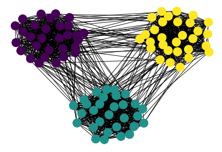
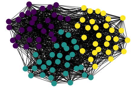
Figure 1: Example graphs with three clusters generated by the stochastic block model (SBM) with the cluster out-density $0.05$ (left subfigure) and $0.2$ (right subfigure).

Table 3: Average ($\pm$ standard deviation) Rand score and computation time of the reference community detection algorithms on the sample of $2{,}880$ test graphs.

Community detection algorithm	Rand score	Time [s]
Greedy Modularity	0.51$\pm$0.35	0.02$\pm$0.04
Label propagation	0.15$\pm$0.26	0.00$\pm$0.00
Leiden	0.66$\pm$0.37	0.00$\pm$0.00
Louvain	0.64$\pm$0.37	0.01$\pm$0.02
Spectral	0.29$\pm$0.23	0.20$\pm$0.22

4.2 Reference results

As a point of reference, let us inspect the following five well-known algorithms: Greedy Modularity Optimisation [16], Label Propagation [17], the Leiden algorithm [60], the Louvain algorithm [5], and standard spectral community detection [22]. The overall results for the reference methods are listed in Table 3.

In line with our expectations, the Leiden and Louvain algorithms achieved the best results, as they are considered state-of-the-art methods for community detection for “regular” graphs. Greedy Modularity Optimisation was also able to yield good results, albeit significantly worse than the mentioned former methods, while the Label propagation algorithm and spectral community detection performed rather unsatisfactorily. We may notice that all of the results are relatively low when compared with the theoretical maximal value of the Rand score equal to 1 – this is due to the presence of particularly challenging test examples in our test set. Specifically, graphs with low both in- and out-density, e.g., in-density equal to 0.4 and out-density equal to 0.3, pose a challenge even for the best community detection algorithms. Therefore, we expect that the average performance of any method will be quite low, and we focus on a pairwise relative comparison of the methods.

When it comes to the run-time comparison, most of the methods generate the community partitioning almost instantaneously, with the spectral community detection being the only exception.

Table 4: Aggregated Rand scores for the considered node dissimilarity-based community detection methods with the Genie clustering. If a certain combination is not reported, it means that the results were unobtainable due to numerical instabilities. “Parameter” denotes the dissimilarity-specific parameter, as listed in Section 4.1. Only the best-performing combinations, with respect to the dissimilarity parameter, are reported.

Dissimilarity	Gini	Param.	Rand score
Blondel–Gajardo	0.3	100	0.02$\pm$0.02
Blondel–Gajardo	0.5	100	0.02$\pm$0.02
K-step probability	0.1	3	0.48$\pm$0.37
K-step probability	0.3	3	0.44$\pm$0.37
K-step probability	0.5	3	0.35$\pm$0.34
Katz index	0.1	0.1	0.30$\pm$0.34
Katz index	0.3	0.1	0.25$\pm$0.30
Katz index	0.5	0.1	0.17$\pm$0.24
Overlap	0.1	-	0.44$\pm$0.40

Dissimilarity	Gini	Param.	Rand score
Overlap	0.3	-	0.42$\pm$0.40
Overlap	0.5	-	0.36$\pm$0.38
PPMI	0.1	1.0	0.50$\pm$0.37
PPMI	0.3	1.0	0.43$\pm$0.36
PPMI	0.5	1.0	0.33$\pm$0.34
Rooted PageRank	0.1	0.3	0.37$\pm$0.29
Wasserman–Faust	0.1	-	0.52$\pm$0.39
Wasserman–Faust	0.3	-	0.47$\pm$0.39
Wasserman–Faust	0.5	-	0.37$\pm$0.37

Table 5: Aggregated Rand scores for the considered node dissimilarity-based community detection methods with the remaining clustering methods.

Dissimilarity	Clustering	Par.	Rand score
Adamic–Adar	Average	-	0.45$\pm$0.43
Adamic–Adar	Complete	-	0.35$\pm$0.43
Adamic–Adar	Single	-	0.16$\pm$0.32
Adamic–Adar	Ward	-	0.53$\pm$0.40
Blondel–Gajardo	Average	1	0.00$\pm$0.01
Blondel–Gajardo	Complete	1	0.00$\pm$0.01
Blondel–Gajardo	Single	1	0.00$\pm$0.00
Blondel–Gajardo	Ward	1	0.01$\pm$0.02
K-step probability	Average	3	0.55$\pm$0.37
K-step probability	Complete	3	0.52$\pm$0.37
K-step probability	Single	3	0.24$\pm$0.37
K-step probability	Ward	3	0.61$\pm$0.33
Katz index	Average	0.1	0.33$\pm$0.36
Katz index	Complete	0.1	0.34$\pm$0.35
Katz index	Single	0.1	0.07$\pm$0.19
Katz index	Ward	0.1	0.42$\pm$0.38

Dissimilarity	Clustering	Par.	Rand score
Overlap	Average	-	0.50$\pm$0.41
Overlap	Complete	-	0.34$\pm$0.43
Overlap	Single	-	0.26$\pm$0.39
Overlap	Ward	-	0.52$\pm$0.40
PPMI	Average	1	0.63$\pm$0.36
PPMI	Complete	1	0.31$\pm$0.42
PPMI	Single	1	0.22$\pm$0.35
PPMI	Ward	1	0.62$\pm$0.36
Rooted PageRank	Average	0.3	0.58$\pm$0.33
Rooted PageRank	Complete	0.3	0.54$\pm$0.33
Rooted PageRank	Single	0.3	0.08$\pm$0.19
Rooted PageRank	Ward	0.3	0.56$\pm$0.33
Wasserman–Faust	Average	-	0.52$\pm$0.41
Wasserman–Faust	Complete	-	0.54$\pm$0.39
Wasserman–Faust	Single	-	0.23$\pm$0.38
Wasserman–Faust	Ward	-	0.60$\pm$0.37

4.3 Node dissimilarity-based community detection

Let us proceed with the analysis of the overall results of the node dissimilarity-based methods. Tables 4 and 5 present the results for the Genie-based implementations and the remaining hierarchical methods, respectively.

The Wasserman–Faust dissimilarity produces the best results when combined with the Genie clustering, but the PPMI-based dissimilarity and the K-step transition probability-based dissimilarity allow the method to achieve relatively high results as well. Overall, only the Blondel–Gajardo matrix seems unsuitable for the dissimilarity-based community detection, as it results in the same performance as random partitioning.

When it comes to the parameters of the Genie clustering, we observe that all of the methods work better for lower values of the inequity threshold. As our test graphs have equal-sized communities, this is expected – any noticeable inequity in the cluster sizes indicates an error in the clustering, and the algorithms aim to fix the error during the process by merging minimum communities.

Analogously, all algorithms have a single parameter value for which they perform the best, regardless of the selected inequity measure and the threshold value. Interestingly, the dissimilarity based on K-step transition probability yields the best results for the lowest value of K, i.e., for the shortest theoretical random walks. This observation suggests that local neighbourhood-sourced dissimilarity conveys the community structure better than the global neighbourhood-sourced one, as would be the case for higher values of K. Similarly, the PPMI-based dissimilarity works best with the continuation probability equal to 1.0, i.e., when a random walk does not randomly return to the source. This result is consistent with intuition, as random returns to the source should only cause undesirable disruptions in conveying the graph’s structure.

By looking at the remaining hierarchical clustering algorithms in Table 5, we observe that the results are relatively consistent, i.e., methods which performed well with Genie clustering also perform well with linkage criteria. In most cases, the average and Ward linkage criteria generate the best results, which is also consistent with our expectations, as they should capture the community similarities the best. We also observe the high performance of the average linkage with PPMI-based dissimilarity, which yields the best performance amongst all node dissimilarity-based methods. We believe it may compete with the state-of-the-art Louvain and Leiden algorithms.

The time comparison shows that most algorithms can generate results almost as quickly as the reference methods. The only exceptions are the methods based on the Wasserman–Faust and the Overlap dissimilarity. This is because these are the only measures for which the dissimilarity matrix must be calculated element-by-element. We can obtain the dissimilarity matrix with algebraic transformations of other graph-related matrices in the remaining cases.

4.4 Spectral-based community detection

In this section, we summarise the results of our spectral-based community methods, which are present in Tables 6 and 7, analogously to the previous section.

None of the methods achieved satisfactory results when compared with our node dissimilarity-based as well as the reference methods. However, this is a somewhat expected phenomenon. When the clustering is performed on the eigenvectors of the graph’s Laplacian matrix, the standard spectral community detection has a proper theoretical justification. Our replacements of the Laplacian matrix do not have the same theoretical justification, but they are still heuristics worth considering.

Most methods gave the same performance quality as a random partitioning – the only exceptions here are the K-step transition probability matrix and the Katz index matrix. More interestingly, the transition matrix’s best parameter value changed from 3 to 5. While we cannot directly deduce why such a change occurred or how the random walk length contributes to the final clustering, it implies that K remains a tunable parameter that impacts the final performance. We repeat the same conclusion for the Katz decay parameter, for whom the best decay parameter value also changed from 0.1 to 0.3.

If we were to try to explain the behaviour of the transition probability-based method, we could notice one fundamental similarity to the Laplacian matrix used for the standard spectral community detection: both the K-step probability matrix and the Laplacian matrix are row-stochastic. While this reasoning has a firm basis, to the best of the authors’ knowledge, this is not the case for the Katz index matrix. Nonetheless, we believe that further research into these two methods can be profitable in terms of understanding spectral community detection better and may yield a new well-performing spectral algorithm in the future.

When we compare the computation time of the methods, only the Overlap and Wasserman–Faust similarity-based methods do not produce the results almost instantaneously due to the need for element-by-element computation. Interestingly, the standard Laplacian matrix can also be obtained from the graph’s adjacency and degree matrix in linear time with respect to the number of vertices. However, when we measure the computation time of the reference spectral method, it requires time similar to the Wasserman–Faust and Overlap-based methods, which in our case is quadratic with respect to the number of vertices. This observation indicates a possibility for improvement in the reference implementation.

Table 6: Aggregated Rand scores for the considered spectral-based community detection methods with Genie clustering.

Similarity	Gini	Param.	Rand score
Adamic–Adar	0.1	-	-0.02$\pm$0.04
Adamic–Adar	0.3	-	-0.01$\pm$0.03
Adamic–Adar	0.5	-	-0.01$\pm$0.03
Blondel–Gajardo	0.1	1	0.03$\pm$0.06
Blondel–Gajardo	0.3	1	0.02$\pm$0.05
Blondel–Gajardo	0.5	1	0.01$\pm$0.04
K-step probability	0.1	5	0.20$\pm$0.17
K-step probability	0.3	5	0.18$\pm$0.16
K-step probability	0.5	5	0.13$\pm$0.13
Katz index	0.1	0.3	0.19$\pm$0.32
Katz index	0.3	0.3	0.18$\pm$0.31
Katz index	0.5	0.3	0.15$\pm$0.28

Similarity	Gini	Param.	Rand score
Overlap	0.1	-	0.00$\pm$0.05
Overlap	0.3	-	0.00$\pm$0.04
Overlap	0.5	-	0.00$\pm$0.03
PPMI	0.1	1.0	0.01$\pm$0.06
PPMI	0.3	1.0	0.01$\pm$0.06
PPMI	0.5	1.0	0.01$\pm$0.04
Rooted PageRank	0.1	0.0	0.02$\pm$0.02
Rooted PageRank	0.3	0.0	0.02$\pm$0.02
Rooted PageRank	0.5	0.0	0.02$\pm$0.02
Wasserman–Faust	0.1	-	0.04$\pm$0.08
Wasserman–Faust	0.3	-	0.04$\pm$0.07
Wasserman–Faust	0.5	-	0.03$\pm$0.06

Table 7: Aggregated Rand scores for the considered spectral-based community detection methods with the remaining clustering methods.

Similarity	Clustering	Par.	Rand score
Adamic–Adar	Average	-	-0.01$\pm$0.03
Adamic–Adar	Complete	-	-0.02$\pm$0.03
Adamic–Adar	Single	-	0.00$\pm$0.01
Adamic–Adar	Ward	-	-0.02$\pm$0.03
Blondel–Gajardo	Average	1	0.01$\pm$0.03
Blondel–Gajardo	Complete	1	0.02$\pm$0.04
Blondel–Gajardo	Single	1	0.01$\pm$0.02
Blondel–Gajardo	Ward	1	0.02$\pm$0.04
K-step probability	Average	5	0.03$\pm$0.06
K-step probability	Complete	5	0.09$\pm$0.10
K-step probability	Single	5	0.01$\pm$0.03
K-step probability	Ward	5	0.16$\pm$0.15
Katz index	Average	0.3	0.18$\pm$0.32
Katz index	Complete	0.3	0.17$\pm$0.31
Katz index	Single	0.3	0.13$\pm$0.27
Katz index	Ward	0.3	0.19$\pm$0.32

Similarity	Clustering	Par.	Rand score
Overlap	Average	-	0.00$\pm$0.02
Overlap	Complete	-	-0.01$\pm$0.03
Overlap	Single	-	0.00$\pm$0.01
Overlap	Ward	-	-0.01$\pm$0.03
PPMI	Average	1.0	0.00$\pm$0.02
PPMI	Complete	1.0	0.00$\pm$0.03
PPMI	Ward	1.0	0.00$\pm$0.03
Rooted PageRank	Average	0.0	0.02$\pm$0.02
Rooted PageRank	Complete	0.0	0.02$\pm$0.02
Rooted PageRank	Single	0.0	0.02$\pm$0.02
Rooted PageRank	Ward	0.0	0.02$\pm$0.02
Wasserman–Faust	Average	-	0.00$\pm$0.01
Wasserman–Faust	Complete	-	0.00$\pm$0.02
Wasserman–Faust	Single	-	0.00$\pm$0.01
Wasserman–Faust	Ward	-	0.00$\pm$0.03

Table 8: Aggregated Rand score and computation times for the considered representation-based community detection methods with the Genie clustering.

Method	Gini	Dim.	Rand score	Time [s]
DNGR	0.1	6	0.57$\pm$0.39	0.87–17.45
DNGR	0.3	6	0.54$\pm$0.39
DNGR	0.5	6	0.47$\pm$0.39
DeepWalk	0.1	6	0.47$\pm$0.37	0.44–4.85
DeepWalk	0.3	6	0.43$\pm$0.35
DeepWalk	0.5	6	0.34$\pm$0.32
GraRep	0.1	6	0.41$\pm$0.40	0.00–1.53
GraRep	0.3	6	0.36$\pm$0.38
GraRep	0.5	6	0.26$\pm$0.33
HOPE	0.1	6	0.30$\pm$0.32	0.00–2.81

Method	Gini	Dim.	Rand score	Time [s]
GF	0.1	12	0.41$\pm$0.36	1.18–2.81
GF	0.3	12	0.36$\pm$0.35
GF	0.5	12	0.27$\pm$0.30
HARP	0.1	6	0.41$\pm$0.36	1.27–17.38
HARP	0.3	6	0.37$\pm$0.34
HARP	0.5	6	0.28$\pm$0.31
Node2Vec	0.1	6	0.47$\pm$0.37	0.48–6.66
Node2Vec	0.3	6	0.43$\pm$0.35
Node2Vec	0.5	6	0.33$\pm$0.32

Table 9: Aggregated Rand scores and computation times for the considered representation-based community detection methods with the remaining clustering methods.

Method	Clust.	D.	Rand s.	Time [s]
DNGR	Average	6	0.53$\pm$0.40	0.83–20.82
DNGR	Complete	6	0.54$\pm$0.38
DNGR	Single	6	0.39$\pm$0.41
DNGR	Ward	6	0.59$\pm$0.39
DeepWalk	Average	6	0.42$\pm$0.38	0.42–4.85
DeepWalk	Complete	6	0.44$\pm$0.35
DeepWalk	Single	6	0.20$\pm$0.32
DeepWalk	Ward	6	0.51$\pm$0.36
GraRep	Average	6	0.25$\pm$0.37	0.00–1.10
GraRep	Complete	6	0.31$\pm$0.34
GraRep	Single	6	0.13$\pm$0.29
GraRep	Ward	6	0.44$\pm$0.40
GF	Average	12	0.28$\pm$0.34	1.17–3.21
GF	Complete	12	0.34$\pm$0.34
GF	Single	12	0.16$\pm$0.28
GF	Ward	12	0.41$\pm$0.35

Method	Clust.	D.	Rand s.	Time [s]
HARP	Average	6	0.35$\pm$0.37	1.25–17.91
HARP	Complete	6	0.38$\pm$0.34
HARP	Single	6	0.17$\pm$0.30
HARP	Ward	6	0.44$\pm$0.36
HOPE	Average	6	0.13$\pm$0.20	0.00–1.13
HOPE	Complete	12	0.14$\pm$0.16
HOPE	Single	6	0.06$\pm$0.17
HOPE	Ward	12	0.29$\pm$0.31
LE	Average	6	0.04$\pm$0.12	0.18–334.79
LE	Complete	6	0.06$\pm$0.15
LE	Single	6	0.02$\pm$0.09
LE	Ward	6	0.08$\pm$0.17
Node2Vec	Average	6	0.45$\pm$0.38	0.48–6.90
Node2Vec	Complete	6	0.45$\pm$0.35
Node2Vec	Single	6	0.21$\pm$0.32
Node2Vec	Ward	6	0.52$\pm$0.36

4.5 Representation-based community detection

Finally, we consider the representation-based community detection methods. The results are presented in Tables 8 and 9, analogously to the previous sections.

We observe that DNGR-based representations yield the best results. DNGR paired with a suitable clustering algorithm is able to achieve only a slightly lower Rand score than the state-of-the-art methods, which we believe is entirely satisfactory. On the other hand, most of the remaining representation learning algorithms give mediocre results. While they outperformed the Label Propagation Algorithm and spectral clustering, they are far behind the Leiden and Louvain algorithms. Among the well-performing algorithms, almost all worked better with six-dimensional representations, which may be explained by the relatively small size of the test graphs. Higher dimensions could be required for larger graphs, where the representation algorithms cannot correctly encode the pairwise node relations.

Comparing the performance as a function of the Gini index threshold and parameter values, we observe the same dependence as in the previous examples: the algorithms work better for lower threshold values, and the best parameter value is independent of the threshold value.

Regarding the computation times, we observe a somewhat expected dependence – factorisation-based algorithms (GraRep, HOPE) generate a partitioning almost instantaneously, while the algorithms requiring explicit optimisation of a given task or training of an underlying neural network need much more time.

5 Detailed evaluation

Based on the results presented in the previous section, we select the following best-performing combinations of methods for further, more detailed analysis:

• Node Genie PPMI – node dissimilarity-based Genie with PPMI-based dissimilarity, the Gini index threshold equal to 0.1, and continuation probability equal to 1,

• Node Genie W-F – node dissimilarity-based Genie with Wasserman–Faust measure-based dissimilarity, and the Gini index threshold equal to 0.1,

• Node Average PPMI – node dissimilarity-based average linkage with PPMI-based dissimilarity, and continuation probability equal to 1,

• Node Average RPR – node dissimilarity-based average linkage with Rooted PageRank-based dissimilarity, and return probability equal to 0.3,

• Spectral Genie K-Step – spectral-based Genie with K-step probability-based similarity, threshold equal to 0.1, and number of steps equal to 5,

• Spectral Ward Katz – spectral-based Ward linkage with Katz index-based similarity, and decay parameter equal to 0.3,

• Euclidean Genie DNGR – representation-based Genie with DNGR representation, threshold equal to 0.1, and embedding dimension equal to 6,

• Euclidean Ward DNGR – representation-based Ward linkage with DNGR representation, and embedding dimension equal to 6,

• Euclidean Ward Node2Vec – representation-based Ward linkage with Node2Vec representation, and embedding dimension equal to 6.

We include the spectral-based methods because while they performed relatively poorly, their analysis is rather interesting based on their observed behaviour.

Let us compare the nine selected methods against the five reference methods listed in Section 4.2. Specifically, we study the performance for various values of the in- and out-densities of the clusters, the performance for various values of the vertex and the cluster number of the graph, and the computation time.

5.1 Graph density-based comparison

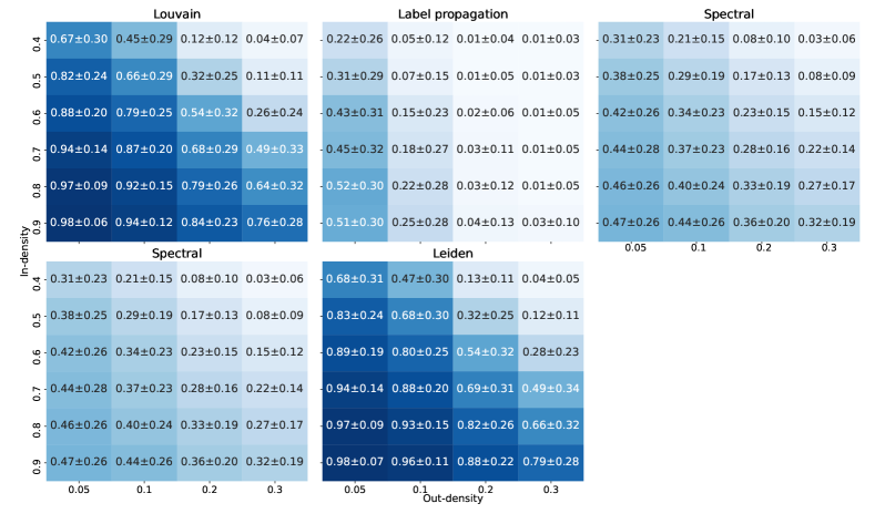
Figure 3: Rand scores with respect to in- and out-density for the selected reference methods.

Firstly, we analyse how our methods behave with respect to various values of in- and out-densities of the clusters in the graph. Figures 2 and 3 present the results for the selected new and the reference methods, respectively.

All node dissimilarity-based and representation-based algorithms behave according to our expectations. They tend to perform better for higher in-densities and lower out-densities of the clusters. We observe that these methods achieve a near-perfect score in the most uncomplicated cases and then gradually decrease in performance as the task complexity increases. Notably, Node Genie PPMI and Node Genie W-F seem to perform relatively poorly for the edge cases, when both in- and out-densities are low – the remaining methods result in the Rand score equal to at least 0.6, while these two produce 0.46 and 0.33, respectively.

Overall, we believe that the most noteworthy results are those related to the spectral-based methods. First, the Spectral Ward Katz seems to work in the same manner as the previously mentioned methods but scored significantly worse. On the other hand, Spectral Genie K-step behaves significantly different – it produces better results when the in-densities are low, and the out-densities are high. Let us stress again, however, that detecting communities with in-densities equal to 0.4 and out-densities equal to 0.3 is exceptionally challenging, as the communities are nearly indistinguishable from their neighbourhood. Therefore, while the Rand score remains low, it is particularly of interest that Spectral Genie K-step outperformed all of the methods, including the reference methods.

Also, looking at the reference methods, we see that the general pattern still holds. The only algorithm that perhaps works somewhat differently is Label Propagation, whose performance seems to depend more firmly on the clusters’ out-densities and less on in-densities. Nonetheless, it performed somewhat poorly, so the grounds for these observations may be unreliable.

In general, we believe that our best method, Node Average PPMI, achieves as good a performance as the best reference methods, i.e., the Louvain and Leiden algorithms: the differences are hardly noticeable. We should also note that our method results in a slightly lower standard deviation of the Rand score for best cases, i.e., that our method correctly detects communities in a more stable manner.

5.2 Cluster structure-based comparison

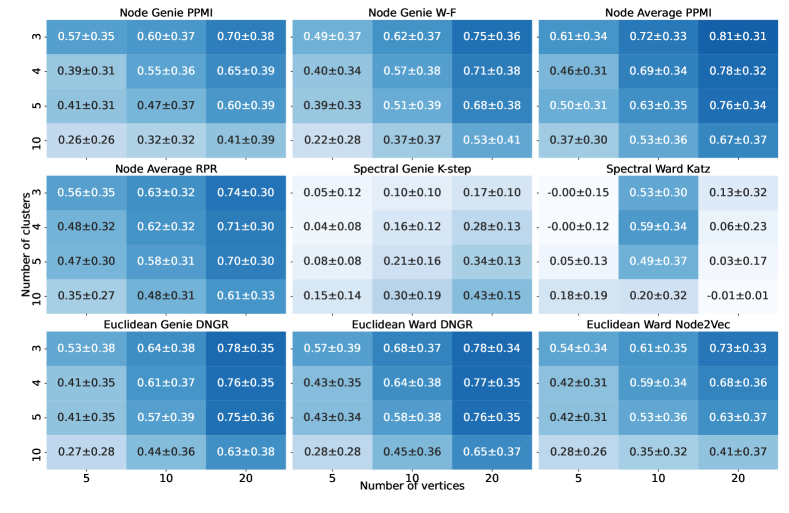
Figure 4: Rand scores with respect to the number of clusters and the number of vertices in a single cluster for the selected new methods.

Secondly, we compare our methods and the reference algorithms with respect to the numbers of vertices in the clusters and the number of clusters. The results are presented in Figures 4 and 5, respectively.

Similarly as in the previous case, if we leave out the spectral-based methods, there are configurations for which the algorithms work better in general. Specifically, all these routines tend to fit better to a low number of large communities. This behaviour is consistent with our expectations, as such configurations are intuitively the easiest to detect: there is a low number of sparse regions in the graph separating the communities, and the communities themselves are clearly distinguishable due to their sizes.

We also once again observe that the spectral-based methods behave in a significantly different manner. Spectral Ward Katz seems to give good results only for some values of the number of vertices and the number of clusters. While this is quite challenging to explain without further analysis reliably, we expect that the parameters of the matrix generation seem to impact the method’s performance significantly for various parameters of the graph. This behaviour is somewhat discouraging when applying this method to an arbitrary dataset, as the results may vary heavily, and we would have no way to distinguish the best partitioning into communities properly. On the other hand, Spectral Genie K-step once again seems to work better in the edge case, where the remaining algorithms work poorly. Specifically, it obtains an almost acceptable Rand score for a large number of big clusters; that is, it can distinguish large communities even when there are many. In this case, it works as good as, e.g., Node Genie PPMI and is better than Greedy Modularity Optimisation but significantly worse than the best algorithms.

If we compare our best method, Node Average PPMI, with the Leiden and Louvain algorithms, we observe that it performs slightly worse in most cases but obtains the best results for many small clusters. As this is the most challenging case, the results suggest that our method may be preferred for some datasets with many communities.

5.3 Real-world datasets

In the last part of the analysis of the results, we compare the performance of our selected methods and reference methods on two previously described datasets, i.e., Zachary’s Karate Club [65] and Lusseau’s Bottlenose Dolphins [42]. As the Dolphins dataset may be partitioned into communities in several ways and there is no one agreed-upon partitioning, we use modularity to evaluate the community detection. The results are presented in Table 10.

When we compare the results on the Karate dataset, we observe that four of our methods significantly outperformed all of the reference methods. It is interesting that the state-of-the-art algorithms, i.e., Louvain and Leiden, could not adequately capture the graph’s community structure, while our algorithms did so very satisfactorily. Also, the spectral-based methods worked poorly, which was expected.

Regarding the Dolphins dataset, the reference methods are better in terms of modularity maximisation. Let us note that this does not indicate that they detected the communities objectively better, only that they seem to yield higher overall modularity, which can be used to evaluate community detection when no ground truth is given. Nonetheless, many of our algorithms achieved only a slightly lower value of the measure.

Table 10: Results of our methods and the reference methods on two real-world datasets: the Rand score and computation time in the Karate task as well as modularity and computation time in the Dolphins task.

Method	$\text{Rand}_{\text{Karate}}$	$\text{T}_{\text{Karate}}$[s]	$\text{Mod}_{\text{Dolphins}}$	$\text{T}_{\text{Dolphins}}$[s]
Node Genie PPMI	0.77	0.01	0.49	0.02
Node Genie W-F	0.88	0.03	0.37	0.02
Node Average PPMI	0.77	0.00	0.49	0.01
Node Average RPR	0.77	0.00	0.38	0.01
Spectral Genie K-step	0.40	0.00	-0.05	0.11
Spectral Ward Katz	-0.01	0.00	0.24	0.01
Euclidean Genie DNGR	0.88	13.86	0.48	19.15
Euclidean Ward DNGR	0.88	11.28	0.48	22.14
Euclidean Ward Node2Vec	0.88	1.21	0.43	1.95
Leiden	0.46	0.00	0.52	0.00
Louvain	0.43	0.00	0.52	0.00
Greedy modularity	0.57	0.00	0.50	0.01
Spectral	0.77	0.05	0.38	0.10
Label propagation	0.38	0.00	0.50	0.00

6 Discussion on Theoretical and Practical Implications

We have developed three general pipelines in which agglomerative hierarchical clustering algorithms may be used for community detection in graphs: node dissimilarity-, spectral-, and representation-based approaches. Each of the pipelines is unique in its own way:

1. node dissimilarity-based approach aims to generalise and build upon the structure of the earliest clustering and community detection algorithms;

2. spectral-based approach tries to verify experimentally whether there is a place for improvement of the standard spectral community detection algorithms;

3. representation-based approach uses the newest, “sophisticated” (black-box) methods based on Graph Representation Learning to propose new ways of performing community detection.

We have tested each pipeline with numerous components and performed a comprehensive analysis of their applicability in the community detection task. Here are the most important outcomes of our analysis.

• Several methods can achieve similar performance as the current state-of-the-art “dedicated” methods, and a majority of our methods significantly outperform older reference algorithms, such as the Label Propagation Algorithm or Greedy Modularity Optimisation. Also, there are instances of graphs on which we obtain better results than the current state-of-the-art.

• In our analysis, we have confirmed the hypothesis regarding the usability of Graph Representation Learning methods for community detection. Specifically, we have shown that some methods, such as Deep Neural Graph Representation (DNGR), can capture the community structure of synthetic and real-world graphs successfully.

• Thanks to developing spectral-based approach, we have observed unexpectedly good performance of selected combinations of tools. We believe that our preliminary results strongly motivate further research into including the K-step walk transition matrices in the spectral community detection process. As we observed, there is a strong premise that such a tool, if improved, may constitute a state-of-the-art algorithm for community detection in sparse graphs with sparse communities.

Moreover, let us emphasise that all of our algorithms are hierarchical. Hence, they present the same advantages as other clustering algorithms from this class. More precisely, the user may select any number of communities, and the communities are interpretable in the sense that we can observe how they decompose into smaller subgraphs. Other standalone methods (e.g., Leiden and Leuven) do not have this property: in their case, the number of clusters must be known in advance, and the $k$-clustering is usually not properly nested or even related to the $l$-clustering, $k\neq l$.

Much work remains to be done in the future, specifically related to spectral-based methods and their applicability. An analysis of synthetic data generated from different models should also be considered.

Conflict of interest

All authors certify that they have no affiliations with or involvement in any organisation or entity with any financial interest or non-financial interest in the subject matter or materials discussed in this manuscript.

Data availability

Zachary’s Karate Club and Dolphins datasets are freely available online. Our battery of synthetic SBM graphs will be made available upon request.

Figure 2: Rand scores with respect to in- and out-density for the selected new methods.

Figure 5: Rand scores with respect to the number of clusters and the number of vertices in a single cluster for the selected reference methods.

References

- Adamic and Adar [2003] Adamic, L.A., Adar, E., 2003. Friends and neighbors on the web. Social Networks 25, 211–230.
- Ahmed et al. [2013] Ahmed, A., Shervashidze, N., Narayanamurthy, S.M., Josifovski, V., Smola, A.J., 2013. Distributed large-scale natural graph factorization, in: WWW ’13: Proceedings of the 22nd international conference on World Wide Web, International World Wide Web Conferences Steering Committee / ACM. pp. 37–48.
- Belkin and Niyogi [2001] Belkin, M., Niyogi, P., 2001. Laplacian eigenmaps and spectral techniques for embedding and clustering, in: NIPS’01: Proceedings of the 14th International Conference on Neural Information Processing Systems: Natural and Synthetic, MIT Press. pp. 585–591.
- Blondel et al. [2004] Blondel, V., Gajardo, A., Heymans, M., Senellart, P., Van Dooren, P., 2004. A measure of similarity between graph vertices: Applications to synonym extraction and web searching. SIAM Review 46, 647–666. doi:10.2307/20453570.
- Blondel et al. [2008] Blondel, V.D., Guillaume, J.L., Lambiotte, R., Lefebvre, E., 2008. Fast unfolding of communities in large networks. Journal of Statistical Mechanics: Theory and Experiment 2008, P10008.
- Bo et al. [2020] Bo, D., Wang, X., Shi, C., Zhu, M., Lu, E., Cui, P., 2020. Structural deep clustering network, in: WWW ’20: Proceedings of The Web Conference 2020, International World Wide Web Conferences Steering Committee / ACM. pp. 1400–1410.
- Brzozowski and Siemaszko [2021] Brzozowski, L., Siemaszko, K., 2021. ReLeGy – Representation learning of graphs in Python. URL: https://github.com/lukaszbrzozowski/ReLeGy.
- Burt [1976] Burt, R.S., 1976. Positions in networks. Social Forces 55, 93–122.
- Cao et al. [2023] Cao, R., Liu, X.F., Fang, Z., Xu, X.K., Wang, X., 2023. How do scientific papers from different journal tiers gain attention on social media? Information Processing & Management 60, 103152. doi:10.1016/J.IPM.2022.103152.
- Cao et al. [2015] Cao, S., Lu, W., Xu, Q., 2015. Grarep: Learning graph representations with global structural information, in: CIKM ’15: Proceedings of the 24th ACM International on Conference on Information and Knowledge Management, ACM. pp. 891–900.
- Cao et al. [2016] Cao, S., Lu, W., Xu, Q., 2016. Deep neural networks for learning graph representations, in: AAAI’16: Proceedings of the Thirtieth AAAI Conference on Artificial Intelligence, AAAI Press. pp. 1145–1152.
- Chen et al. [2021] Chen, D., Nie, M., Wang, J., Kong, Y., Wang, D., Huang, X., 2021. Community detection based on graph representation learning in evolutionary networks. Applied Sciences 11.
- Chen et al. [2018] Chen, H., Perozzi, B., Hu, Y., Skiena, S., 2018. Harp: Hierarchical representation learning for networks, in: AIES ’18: Proceedings of the 2018 AAAI/ACM Conference on AI, Ethics, and Society, AAAI Press. pp. 2127–2134.
- Chen et al. [2022] Chen, H., Yu, Z., Yang, Q., Shao, J., 2022. Community detection in subspace of attribute. Information Sciences 602, 220–235. doi:10.1016/j.ins.2022.04.047.
- Church and Hanks [1989] Church, K.W., Hanks, P., 1989. Word association norms, mutual information and lexicography, in: ACL ’89: Proceedings of the 27th annual meeting on Association for Computational Linguistics, ACL. pp. 76–83.
- Clauset et al. [2004] Clauset, A., Newman, M.E.J., Moore, C., 2004. Finding community structure in very large networks. Phys. Rev. E 70, 066111. doi:10.1103/PhysRevE.70.066111.
- Cordasco and Gargano [2011] Cordasco, G., Gargano, L., 2011. Community detection via semi-synchronous label propagation algorithms. 2010 IEEE International Workshop on Business Applications of Social Network Analysis, BASNA 2010 , 1–8.
- Dekker et al. [2022] Dekker, M.M., Medvedev, A.N., Rombouts, J., Siudem, G., Tupikina, L., 2022. Modelling railway delay propagation as diffusion-like spreading. EPJ Data Sci. 11, 44. doi:10.1140/epjds/s13688-022-00359-1.
- Donnat et al. [2018] Donnat, C., Zitnik, M., Hallac, D., Leskovec, J., 2018. Learning structural node embeddings via diffusion wavelets, in: KDD ’18: Proceedings of the 24th ACM SIGKDD International Conference on Knowledge Discovery and Data Mining, ACM. pp. 1320–1329.
- Erdös and Rényi [1959] Erdös, P., Rényi, A., 1959. On random graphs I. Publicationes Mathematicae Debrecen 6, 290.
- Fani et al. [2020] Fani, H., Jiang, E., Bagheri, E., Al-Obeidat, F., Du, W., Kargar, M., 2020. User community detection via embedding of social network structure and temporal content. Information Processing & Management 57, 102056. doi:10.1016/j.ipm.2019.102056.
- Filippone et al. [2008] Filippone, M., Camastra, F., Masulli, F., Rovetta, S., 2008. A survey of kernel and spectral methods for clustering. Pattern Recognition 41, 176–190.
- Fortunato [2010] Fortunato, S., 2010. Community detection in graphs. Physics Reports 486, 75–174. doi:10.1016/j.physrep.2009.11.002.
- Fortunato and Newman [2022] Fortunato, S., Newman, M.E., 2022. 20 years of network community detection. Nature Physics 18, 848–850.
- Gagolewski [2021] Gagolewski, M., 2021. genieclust: Fast and robust hierarchical clustering. SoftwareX 15, 100722. doi:10.1016/j.softx.2021.100722.
- Gagolewski [2022] Gagolewski, M., 2022. Adjusted asymmetric accuracy: A well-behaving external cluster validity measure. URL: https://arxiv.org/pdf/2209.02935.pdf, doi:10.48550/arXiv.2209.02935. under review (preprint).
- Gagolewski et al. [2016] Gagolewski, M., Bartoszuk, M., Cena, A., 2016. Genie: A new, fast, and outlier-resistant hierarchical clustering algorithm. Information Sciences 363, 8–23.
- Garey and Johnson [1979] Garey, M.R., Johnson, D.S., 1979. Computers and Intractability: A Guide to the Theory of NP-Completeness. W. H. Freeman.
- Girvan and Newman [2002] Girvan, M., Newman, M.E.J., 2002. Community structure in social and biological networks. Proceedings of the National Academy of Sciences 99, 7821–7826.
- Godsil and Royle [2001] Godsil, C.D., Royle, G.F., 2001. Algebraic Graph Theory. Springer.
- Golub and Reinsch [1970] Golub, G.H., Reinsch, C., 1970. Singular value decomposition and least squares solutions. Numer. Math. 14, 403–420.
- Grover and Leskovec [2016] Grover, A., Leskovec, J., 2016. Node2vec: Scalable feature learning for networks, in: KDD ’16: Proceedings of the 22nd ACM SIGKDD International Conference on Knowledge Discovery and Data Mining, ACM. pp. 855–864.
- Hamdaqa et al. [2014] Hamdaqa, M., Tahvildari, L., LaChapelle, N., Campbell, B., 2014. Cultural scene detection using reverse Louvain optimization. Sci. Comput. Program. 95, 44–72.
- Hamilton et al. [2017] Hamilton, W.L., Ying, R., Leskovec, J., 2017. Representation learning on graphs: Methods and applications. IEEE Data Eng. Bull. 40, 52–74.
- He et al. [2022] He, C., Zheng, Y., Cheng, J., Tang, Y., Chen, G., Liu, H., 2022. Semi-supervised overlapping community detection in attributed graph with graph convolutional autoencoder. Information Sciences 608, 1464–1479. doi:10.1016/j.ins.2022.07.036.
- Holland et al. [1983] Holland, P.W., Laskey, K.B., Leinhardt, S., 1983. Stochastic blockmodels: First steps. Social Networks 5, 109–137.
- Hu et al. [2022] Hu, D., Feng, D., Xie, Y., 2022. Egc: A novel event-oriented graph clustering framework for social media text. Information Processing & Management 59, 103059. doi:10.1016/J.IPM.2022.103059.
- Katz [1953] Katz, L., 1953. A new status index derived from sociometric analysis. Psychometrika 18, 39–43.
- Kipf and Welling [2016] Kipf, T.N., Welling, M., 2016. Variational graph auto-encoders. CoRR abs/1611.07308.
- Kipf and Welling [2017] Kipf, T.N., Welling, M., 2017. Semi-supervised classification with graph convolutional networks, in: ICLR ’17: Proceedings of the 5th International Conference on Learning Representations, OpenReview.net.
- Lawrence and Phipps [1985] Lawrence, H., Phipps, A., 1985. Comparing partitions. Journal of Classification 2, 193–218.
- Lusseau [2003] Lusseau, D., 2003. The emergent properties of a dolphin social network. Proc. Biol. Sci. 270 Suppl 2, S186–8.
- Mancoridis et al. [1998] Mancoridis, S., Mitchell, B.S., Rorres, C., Chen, Y.F., Gansner, E.R., 1998. Using Automatic Clustering to Produce High-Level System Organizations of Source Code, in: IWPC ’98: Proceedings of the 6th International Workshop on Program Comprehension, IEEE. pp. 45–52.
- Mikolov et al. [2013] Mikolov, T., Chen, K., Corrado, G., Dean, J., 2013. Efficient estimation of word representations in vector space, in: ICLR ’13: Proceedings of the 1st International Conference on Learning Representations.
- Murtagh [1983] Murtagh, F., 1983. A survey of recent advances in hierarchical clustering algorithms. The Computer Journal 26, 354–359.
- Newman and Girvan [2004] Newman, M.E.J., Girvan, M., 2004. Finding and evaluating community structure in networks. Phys. Rev. E 69, 026113.
- Osiński et al. [2004] Osiński, S., Stefanowski, J., Weiss, D., 2004. Lingo: Search results clustering algorithm based on singular value decomposition, in: Kłopotek, M.A., Wierzchoń, S.T., Trojanowski, K. (Eds.), Intelligent Information Processing and Web Mining, Springer Berlin Heidelberg. pp. 359–368.
- Ou et al. [2016] Ou, M., Cui, P., Pei, J., Zhang, Z., Zhu, W., 2016. Asymmetric transitivity preserving graph embedding, in: KDD ’16: Proceedings of the 22nd ACM SIGKDD International Conference on Knowledge Discovery and Data Mining, ACM. pp. 1105–1114.
- Page et al. [1999] Page, L., Brin, S., Motwani, R., Winograd, T., 1999. The PageRank Citation Ranking: Bringing Order to the Web. Technical Report 1999-66. Stanford InfoLab.
- Patnaik et al. [2016] Patnaik, A.K., Bhuyan, P.K., Krishna Rao, K., 2016. Divisive analysis (diana) of hierarchical clustering and gps data for level of service criteria of urban streets. Alexandria Engineering Journal 55, 407–418.
- Paul and Chen [2016] Paul, S., Chen, Y., 2016. Null models and modularity based community detection in multi-layer networks. Sankhya A 84. doi:10.1007/s13171-021-00257-0.
- Perozzi et al. [2014] Perozzi, B., Al-Rfou, R., Skiena, S., 2014. Deepwalk: Online learning of social representations, in: KDD ’14: Proceedings of the 20th ACM SIGKDD International Conference on Knowledge Discovery and Data Mining, ACM. pp. 701–710.
- Révész [1990] Révész, P., 1990. Random Walk in Random and Non-Random Environments. World Scientific.
- Rezaei and Fränti [2016] Rezaei, M., Fränti, P., 2016. Set matching measures for external cluster validity. IEEE Transactions on Knowledge and Data Engineering 28, 2173–2186. doi:10.1109/TKDE.2016.2551240.
- Ribeiro et al. [2017] Ribeiro, L.F.R., Saverese, P.H.P., Figueiredo, D.R., 2017. Struc2vec: Learning node representations from structural identity, in: KDD ’17: Proceedings of the 23rd ACM SIGKDD International Conference on Knowledge Discovery and Data Mining, ACM. pp. 385–394.
- Sieranoja and Fränti [2022] Sieranoja, S., Fränti, P., 2022. Adapting k-means for graph clustering. Knowledge and Information Systems 64, 115–142. doi:10.1007/S10115-021-01623-Y.
- Su et al. [2022] Su, X., Xue, S., Liu, F., Wu, J., Yang, J., Zhou, C., Hu, W., Paris, C., Nepal, S., Jin, D., Sheng, Q.Z., Yu, P.S., 2022. A comprehensive survey on community detection with deep learning. IEEE transactions on neural networks and learning systems PP. doi:10.1109/TNNLS.2021.3137396.
- Sun et al. [2019] Sun, F.Y., Qu, M., Hoffmann, J., Huang, C., Tang, J., 2019. vGraph: A Generative Model for Joint Community Detection and Node Representation Learning, in: NIPS’18: Proceedings of the 32nd International Conference on Neural Information Processing Systems, pp. 512–522.
- Tang et al. [2015] Tang, J., Qu, M., Wang, M., Zhang, M., Yan, J., Mei, Q., 2015. Line: Large-scale information network embedding, in: WWW ’15 Companion: Proceedings of the 24th International Conference on World Wide Web, International World Wide Web Conferences Steering Committee / ACM. pp. 1067–1077.
- Traag et al. [2019] Traag, V., Waltman, L., van Eck, N.J., 2019. From Louvain to Leiden: Guaranteeing well-connected communities. Scientific Reports 9, 5233. doi:10.1038/s41598-019-41695-z.
- Wang et al. [2016] Wang, D., Cui, P., Zhu, W., 2016. Structural deep network embedding, in: KDD ’16: Proceedings of the 22nd ACM SIGKDD International Conference on Knowledge Discovery and Data Mining, ACM. pp. 1225–1234.
- Wasserman and Faust [1994] Wasserman, S., Faust, K., 1994. Social Network Analysis: Methods and Applications. Cambridge University Press.
- Wilinski et al. [2019] Wilinski, M., Mazzarisi, P., Tantari, D., Lillo, F., 2019. Detectability of macroscopic structures in directed asymmetric stochastic block model. Physical Review E 99, 042310.
- Xu and Tian [2015] Xu, D., Tian, Y., 2015. A comprehensive survey of clustering algorithms. Annals of Data Science 2, 165–193.
- Zachary [1977] Zachary, W.W., 1977. An information flow model for conflict and fission in small groups. Journal of Anthropological Research 33, 452–473.
- Zhang et al. [2012] Zhang, W., Wang, X., Zhao, D., Tang, X., 2012. Graph degree linkage: Agglomerative clustering on a directed graph, in: ECCV’12: Proceedings of the 12th European conference on Computer Vision, Springer. pp. 428–441.
- Zhang et al. [2022] Zhang, Y., Pietrasik, M., Xu, W., Reformat, M., 2022. Hierarchical topic modelling for knowledge graphs. Lecture Notes in Computer Science (including subseries Lecture Notes in Artificial Intelligence and Lecture Notes in Bioinformatics) 13261 LNCS, 270–286. doi:10.1007/978-3-031-06981-9_16.