Portfolio Optimization with Relative Tail Risk

Abstract

This paper proposes analytic forms of portfolio CoVaR and CoCVaR on the normal tempered stable market model. Since CoCVaR captures the relative risk of the portfolio with respect to a benchmark return, we apply it to the relative portfolio optimization. Moreover, we derive analytic forms for the marginal contribution to CoVaR and the marginal contribution to CoCVaR. We discuss the Monte-Carlo simulation method to calculate CoCVaR and the marginal contributions of CoVaR and CoCVaR. As the empirical illustration, we show relative portfolio optimization with thirty stocks under the distress condition of the Dow Jones Industrial Average. Finally, we perform the risk budgeting method to reduce the CoVaR and CoCVaR of the portfolio based on the marginal contributions to CoVaR and CoCVaR.
Key words: Portfolio Optimization Relative Risk Normal Tempered Stable Model CoVaR CoCVaR Marginal Contribution to Risk

1 Introduction

Harry Markowitz’s mean-variance portfolio optimization technique (Markowitz (1952)) has made a remarkable impact on portfolio theory in finance. This innovative method has been extensively utilized successfully in portfolio selection, allocation, and risk management practices. The adoption of Markowitz’s mean-variance model has resulted in significant improvements in investment outcomes and become a cornerstone of modern portfolio theory. Many investors have utilized Markowitz’s method to determine an efficient portfolio weight vector. Still, constructing a portfolio that surpasses the market index (e.g., S&P 500 index or DJIA) is not easy to be achieved. For that reason, some investors use relative portfolio optimization, that is, relaxing the assumption of the portfolio variance as the tracking error, which is a variance of the relative return. Here, the relative return is the difference between the portfolio return and a benchmark return, such as the market index return

This paper presents how to improve relative portfolio optimization based on two aspects. First, we loosen the Gaussian assumption of Markowitz’s model, which was empirically rejected in literature including Fama (1963), Mandelbrot (1963a, b), and Cont and Tankov (2004). Non-Gaussian multivariate distributions have been introduced to capture stylized facts, such as fat-tails and asymmetric dependence, that are not accounted for by the Gaussian model. This paper proposes the normal tempered stable (NTS) distribution as an alternative distribution to the Gaussian distribution. The NTS is defined by the tempered stable subordinated Gaussian distribution (Barndorff-Nielsen (1978), Barndorff-Nielsen and Levendorskii (2001) and Barndorff-Nielsen and Shephard (2001)). The NTS distribution has been popularly applied in finance by capturing the fat-tails of the asset return distribution and describing asymmetric dependence (See Kim and Volkmann (2013)). For example, it is applied to financial risk management in Anand et al. (2017) and Kurosaki and Kim (2018), and portfolio management in Eberlein and Madan (2010), Anand et al. (2016), and Kim (2022). In addition, Kim et al. (2015) applies a Lévy  process generated by the two-dimensional NTS distribution to Quanto option pricing, and its extension to capture stochastic dependence is further discussed in Kim et al. (2023). Recently, the NTS distribution was applied to cryptocurrency portfolio optimization in Kurosaki and Kim (2022).

Second, we enhance the portfolio theory by replacing CoVaR and CoCVaR instead of the variance of the relative return as the risk measure. Traditionally, portfolio variance, value at risk (VaR), and conditional value at risk (CVaR) have been employed as the portfolio risk measure, but those are absolute risk measures. Relative traders prefer to use tracking errors such as the variance of relative return with respect to the benchmark return instead of the absolute risk measures. In this paper, we take CoVaR (Adrian and Brunnermeier (2016)) and CoCVaR (Huang and Uryasev (2018)) as the risk measures of relative portfolio optimization. CoVaR is proposed as a measure of systemic risk, which is the VaR of the financial system under the condition of a distressed market. Girardi and Tolga Ergün (2013) calculate CoVaR on the multivariate GARCH model and Reboredo and Ugolini (2015) use the copula method. CoCVaR (or CoES by Adrian and Brunnermeier (2016)) is an expected downturn of the financial system under the condition of a distressed market. Huang and Uryasev (2018) define the mathematical formula of CoCVaR and apply it to measure the risk of the ten largest publicly traded banks in the United States under a distressed condition of market factors. Recently, Liu et al. (2021) discuss CoVaR and CoCVaR on the GARCH model with two-dimensional NTS innovations and do the back-testing.

The paper discusses portfolio optimization minimizing the portfolio CoVaR and CoCVaR concerning the market index and derives the marginal contributions to risk for the portfolio CoVaR and CoCVaR. The marginal contribution to risk is the rate of change in risk with respect to a small percentage change in proportion to a member’s asset. Mathematically it is defined by the first derivative of CoVaR or CoCVaR with respect to the marginal weight. In the context of absolute optimization, the marginal contributions to VaR and CVaR are employed to identify assets with high and low levels of risk. The general form of marginal risk contributions for the VaR and CVaR are provided in Gourieroux et al. (2000). The analytic forms of the marginal contributions for VaR and CVaR are discussed under the skewed-$t$ distribution in Stoyanov et al. (2013), and under the NTS distribution in Kim et al. (2012) and Kim (2022). Since we focus on relative optimization in this paper, we provide analytic formulas for the marginal contributions to CoVaR and CoCVaR under the NTS market model instead of VaR and CVaR. Those marginal contributions to CoVaR and CoCVaR help relative traders to make decisions in portfolio rebalancing. However, the multiple integrals involved in these formulas can present technical difficulties for numerical calculations. To solve this problem, we use Monte-Carlo simulation (MCS) methods. Furthermore, we perform the risk budgeting based on the marginal contributions to CoVaR and CVaR empirically.

The remainder of this paper is organized as follows. The definition of portfolio CoVaR and portfolio CoCVaR are presented in Section 2. Section 3 reviews the NTS market model. Section 4 presents the portfolio CoVaR and CoCVaR on the NTS market model, along with a detailed analysis of the marginal contributions to CoVaR and CoCVaR. Empirical illustrations are given in section 5. In this section, we exhibit MCS method to calculate CoCVaR on the NTS market model and do the portfolio CoCVaR minimizing portfolio optimization with the estimated parameters. We also discuss portfolio budgeting using the marginal CoVaR and the marginal CoCVaR. Finally, Section 6 concludes. Proofs and mathematical details are presented in Appendix.

2 CoVaR and CoCVaR

Let $X$ be a random variable for a market factor, for instance, the market index returns, and $Y$ be a random variable for asset or portfolio returns. We consider a random vector $(X,Y)$ following a joint distribution. The CoVaR and CoCVaR of $Y$ at a significant level $\eta$ under a condition of the event $X\leq-\textup{\rm VaR}_{\zeta}(X)$ are defined by

$$\textup{\rm CoVaR}_{{\eta},{\zeta}}\left({{Y}|{X}}\right)=\textup{\rm VaR}_{\eta}(Y|X\leq-\textup{\rm VaR}_{\zeta}(X))=-\inf_{x}\{x|P(Y\leq x|X\leq-\textup{\rm VaR}_{\zeta}(X))\geq\eta\},$$

and

$$\textup{\rm CoCVaR}_{{\eta},{\zeta}}\left({{Y}|{X}}\right)=-E\left[Y|Y<-\textup{\rm CoVaR}_{{\eta},{\zeta}}\left({{Y}|{X}}\right),X\leq-\textup{\rm VaR}_{\zeta}(X)\right],$$

respectively, where $\textup{\rm VaR}_{\zeta}(X)$ is the Value-at-Risk (VaR) of $X$ for a significant level $\zeta$ given as

$$\textup{\rm VaR}_{\zeta}(X)=-\inf_{x}\{x|P\left(X\leq x\right)\geq\zeta\}.$$

If the joint distribution of $(X,Y)$ is continuous, then $\textup{\rm VaR}_{\zeta}(X)=-F_{X}^{-1}(\zeta)$ where $F_{X}$ is the cumulative distribution function (cdf) for the marginal distribution of $X$ and $F_{X}^{-1}$ is the inverse function of $F_{X}$. Moreover, we have

$$F_{(X,Y)}(-\textup{\rm VaR}_{\zeta}(X),-\textup{\rm CoVaR}_{{\eta},{\zeta}}\left({{Y}|{X}}\right))=\eta\zeta$$

for the joint cdf of $(X,Y)$.

Consider $N$ number of stocks and a market index and an $(N+1)$-dimensional random vector $R=(R_{0}$, $R_{1}$, $\cdots$, $R_{N})^{{\texttt{T}}}$, where $R_{0}$ is the index return and $R_{n}$ is the return of the $n$th stock for $n\in\{1$, $2$, $\cdots$, $N\}$. Let $w=(w_{1}$, $w_{2}$, $\cdots$, $w_{N})^{\texttt{T}}\in I^{N}$ be an $N$-dimensional vector satisfying $\sum_{n=1}^{N}w_{n}=1$ for $I=[0,1]$. The $n$th element $w_{n}$ of $w$ is the proportion of capital invested in the $n$th stock for $n\in\{1,2,\cdots,N\}$. In this case, $w$ be referred to as the capital allocation weight vector for the $N$ stocks in the market. Then we have the random variable of the portfolio return as $R_{p}(w)=\sum_{n=1}^{N}w_{n},R_{n}$.

Suppose that $R$ follows $(N+1)$-dimensional normal distribution with a mean vector $\mu=(\mu_{0}$, $\mu_{1}$, $\cdots$, $\mu_{N})^{\texttt{T}}$ and a covariance matrix $\Sigma$, that is $R\sim\Phi(\mu,\Sigma)$. Let $\sigma_{n,m}$ be the $(n+1,m+1)$-th element of $\Sigma$ for $n,m\in\{0,1,\cdots,N\}$. Then the bivariate random vector $(R_{0},R_{p}(w))^{\texttt{T}}$ follows the bivariated normal distribution, $(R_{0},R_{p}(w))^{\texttt{T}}\sim\Phi(\bar{\mu},\bar{\Sigma})$ with

$$\bar{\mu}=(\mu_{0},\mu_{p}(w))^{\texttt{T}},\text{ and }\bar{\Sigma}=\left(\begin{matrix}\sigma_{0,0}&\sigma_{p,0}(w)\\ \sigma_{p,0}(w)&\sigma_{p}^{2}(w)\end{matrix}\right),$$

where $\mu_{p}(w)=\sum_{n=1}^{N}w_{n}\mu_{n}$, $\sigma_{p,0}(w)=\sum_{n-1}^{N}w_{m}\sigma_{0,n}$, $\sigma_{p}^{2}(w)=\sum_{n=1}^{N}\sum_{m=1}^{N}w_{m}w_{m}\sigma_{n,m}$. We can calculate VaR of $R_{0}$ as $\textup{\rm VaR}_{\zeta}(R_{0})=q_{1-\zeta}\sqrt{\sigma_{0,0}}-\mu_{0}$, where $q_{1-\zeta}$ is $(1-\zeta)$-quantile value of the standard normal distribution. Suppose the value $x$ satisfies

$$\int_{-\infty}^{x}\int_{-\infty}^{-\textup{\rm VaR}_{\zeta}(R_{0})}f_{\Phi(\bar{\mu},\bar{\Sigma})}(x_{1},x_{2})dx_{1}dx_{2}=\eta\zeta,$$

where $f_{\Phi(\bar{\mu},\bar{\Sigma})}$ is the probability density function of $\Phi(\bar{\mu},\bar{\Sigma})$. Then $\textup{\rm CoVaR}_{{\eta},{\zeta}}\left({{R_{p}(w)}|{R_{0}}}\right)=-x$. Moreover,

$$\textup{\rm CoCVaR}_{{\eta},{\zeta}}\left({{R_{p}(w)}|{R_{0}}}\right)=-\frac{1}{\eta\zeta}\int_{-\infty}^{-\textup{\rm CoVaR}_{{\eta},{\zeta}}\left({{R_{p}(w)}|{R_{0}}}\right)}\int_{-\infty}^{-\textup{\rm VaR}_{\zeta}(R_{0})}x_{1}f_{\Phi(\bar{\mu},\bar{\Sigma})}(x_{1},x_{2})dx_{1}dx_{2}.$$

3 Standard NTS distribution and NTS Market model

In this section, we define the multivariate standard NTS distribution and construct the market model based on the distribution.

3.1 Standard NTS Distribution

Let $N$ be a finite positive integer and $\Xi=(\Xi_{1},\Xi_{2},\cdots,\Xi_{N})^{{\texttt{T}}}$ be a multivariate random variable given by

$$\Xi=\beta({\mathcal{T}}-1)+\textup{diag}(\gamma)\varepsilon\sqrt{{\mathcal{T}}},$$

where

• ${\mathcal{T}}$ is the tempered stable subordinator with parameters $(\alpha,\theta)$, and is independent of $\varepsilon_{n}$ for all $n=1,2,\cdots,N$.

• $\beta=(\beta_{1},\beta_{2},\cdots,\beta_{N})^{{\texttt{T}}}\in\mathbb{R}^{N}$ with $|\beta_{n}|<\sqrt{\frac{2\theta}{2-\alpha}}$ for all $n\in\{1,2,\cdots,N\}$.

• $\gamma=(\gamma_{1},\gamma_{2},\cdots,\gamma_{N})^{{\texttt{T}}}\in\mathbb{R}_{+}^{N}$ with $\gamma_{n}=\sqrt{1-\beta_{n}^{2}\left(\frac{2-\alpha}{2\theta}\right)}$ for all $n\in\{1,2,\cdots,N\}$ and $\mathbb{R}_{+}=[0,\infty)$.

• $\varepsilon=(\varepsilon_{1},\varepsilon_{2},\cdots,\varepsilon_{N})^{{\texttt{T}}}$ is $N$-dimensional standard normal distribution with a covariance matrix $\Sigma$. That is, $\varepsilon_{n}\sim\Phi(0,1)$ for $n\in\{1,2,\cdots,N\}$ and $(k,l)$-th element of $\Sigma$ is given by $\rho_{k,l}=\textrm{\rm cov}(\varepsilon_{k},\varepsilon_{l})$ for $k,l\in\{1,2,\cdots,N\}$. Note that $\rho_{k,k}=1$.

In this case, $\Xi$ is referred to as the $N$-dimensional standard NTS random variable with parameters $(\alpha$, $\theta$, $\beta$, $\Sigma)$ and we denote it by $\Xi\sim\textup{stdNTS}_{N}(\alpha$, $\theta$, $\beta$, $\Sigma)$ (See more details in Kim and Volkmann (2013) and Kim (2022).).

• The probability density function (pdf) $f_{\mathcal{T}}(t)$ of ${\mathcal{T}}$ is $f_{\mathcal{T}}(t)=\frac{1}{2\pi}\int_{-\infty}^{\infty}e^{-iut}\phi_{\mathcal{T}}(u)du$, where $\phi_{{\mathcal{T}}}$ is the characteristic function (ch.f) of ${\mathcal{T}}$ given by $\phi_{{\mathcal{T}}}(u)=\exp\left(-\frac{2\theta^{1-\frac{\alpha}{2}}}{\alpha}\left((\theta-iu)^{\frac{\alpha}{2}}-\theta^{\frac{\alpha}{2}}\right)\right).$

• The cdf of the stdNTS vector $\Xi$ is given by

  $$F_{\Xi}(a_{1},\cdots,a_{N})=\int_{0}^{\infty}\int_{-\infty}^{\frac{a_{N}-\beta_{N}(t-1)}{\gamma_{N}\sqrt{t}}}\cdots\int_{-\infty}^{\frac{a_{1}-\beta_{1}(t-1)}{\gamma_{1}\sqrt{t}}}f_{\varepsilon}(x_{1},\cdots,x_{N})dx_{1}\cdots dx_{N}f_{\mathcal{T}}(t)dt,$$ (1)

  where $f_{\varepsilon}$ is the pdf of $N$-dimensional normal distribution with mean $0$ and covariance $\Sigma$.

• The pdf if the vector $\Xi$ is given by

  $$f_{\Xi}(x_{1},\cdots,x_{N})=\int_{0}^{\infty}f_{\Phi(m(t),\Sigma(t))}(x_{1},\cdots,x_{N})f_{\mathcal{T}}(t)dt$$ (2)

  where $f_{\Phi(m(t),\Sigma(t))}(x_{1},\cdots,x_{N})$ is the pdf of the $N$-dimensional normal distribution with mean $m(t)=(\beta_{1}(t-1),\cdots,\beta_{N}(t-1))$ and covariance $\Sigma(t)=\left(t\gamma_{k}\gamma_{l}\rho_{k,l}\right)_{k,l\in\{1,\cdots,N\}}$.

• By Gil-Pelaez (1951), the marginal cdf of $\Xi_{n}$ for $n\in\{1,2,\cdots,N\}$ is equal to

  $$F_{\Xi_{n}}(x)=\frac{1}{2}-\frac{1}{\pi}\int_{-\infty}^{\infty}\frac{\textrm{\rm Im}(e^{-iux}\phi_{\Xi_{n}}(u))}{u}du.$$ (3)

  where $\phi_{\Xi_{n}}$ is the ch.f of $\Xi_{n}$ given by

  $$\phi_{\Xi_{n}}(u) =\exp\left(-\beta_{n}iu-\frac{2\theta^{1-\frac{\alpha}{2}}}{\alpha}\left(\left(\theta-i\beta_{n}u+\frac{u^{2}}{2}\left(1-\beta_{n}^{2}\left(\frac{2-\alpha}{2\theta}\right)\right)\right)^{\frac{\alpha}{2}}-\theta^{\frac{\alpha}{2}}\right)\right).$$

  Moreover, the marginal pdf of $\Xi_{n}$ is obtained by the inverse Fourier transform for the characteristic function as

  $$f_{\Xi_{n}}(x)=\frac{1}{2\pi}\int_{-\infty}^{\infty}e^{-iux}\phi_{\Xi_{n}}(u)du.$$

• Covariance between $\Xi_{n}$ and $\Xi_{m}$ for $n,m\in\{1,2,\cdots,N\}$ is equal to

  $$\textrm{\rm cov}(\Xi_{n},\Xi_{m})=\gamma_{n}\gamma_{m}\rho_{n,m}+\beta_{n}\beta_{m}\left(\frac{2-\alpha}{2\theta}\right).$$ (4)

3.2 NTS Market Model

Consider a portfolio having $N$ assets for a positive integer $N$. The return of the assets in the portfolio is given by a random vector $R=(R_{1}$, $R_{2}$, $\cdots$, $R_{N})^{\texttt{T}}$. We suppose that the return $R$ follows

$$R=\mu+\textrm{\rm diag}(\sigma)\Xi$$ (5)

where $\mu=(\mu_{1},\mu_{2},\cdots,\mu_{N})^{\texttt{T}}\in\mathbb{R}^{N}$, $\sigma=(\sigma_{1},\sigma_{2},\cdots,\sigma_{N})^{\texttt{T}}\in\mathbb{R}_{+}^{N}$ and $\Xi\sim\textup{\rm stdNTS}_{N}(\alpha,\theta,\beta,\Sigma)$. Then, we have $E[R_{n}]=\mu_{n}$ and $\textrm{\rm var}(R_{n})=\sigma_{n}^{2}$ for all $n\in\{1,2,\cdots,N\}$. This market model is referred to as the NTS market model.

Let $w=(w_{1},w_{2},\cdots,w_{N})^{\texttt{T}}$ be the capital allocation weight vector. Then the portfolio return for $w$ is equal to $R_{P}(w)=w^{\texttt{T}}R$. The distribution of $R_{P}(w)$ is presented in the following proposition from Kim (2022).

Proposition 3.1 (Kim (2022)).

Consider a portfolio with $N$ assets for a positive integer $N$. Let $w=(w_{1}$, $w_{2}$, $\cdots$, $w_{N})^{{\texttt{T}}}$ be the capital allocation weight vector for the portfolio. Suppose $R=(R_{1}$, $R_{2}$, $\cdots$, $R_{N})^{\texttt{T}}\in\mathbb{R}^{N}$ follows the NTS market model given by (5) with $\mu\in\mathbb{R}^{N}$, $\sigma\in\mathbb{R}_{+}^{N}$, and $\Xi\sim\textup{stdNTS}_{N}(\alpha,\theta,\beta,\Sigma)$. Then

$$R_{P}(w)\stackrel{{\scriptstyle\mathrm{d}}}{{=}}\bar{\mu}(w)+\bar{\sigma}(w)\Xi~{}~{}~{}\text{ for }~{}~{}~{}\Xi\sim\textup{stdNTS}_{1}(\alpha,\theta,\bar{\beta}(w),1),$$ (6)

where

$$\bar{\mu}(w)=\sum_{n=1}^{N}w_{n}\mu_{n},~{}~{}~{}\bar{\sigma}(w)=\sqrt{\sum_{n=1}^{N}w_{n}\sum_{m=1}^{N}w_{n}w_{m}\textrm{\rm cov}(R_{n},R_{m})},~{}~{}~{}\text{and}~{}~{}~{}\bar{\beta}(w)=\frac{\sum_{n=1}^{N}w_{n}\sigma_{n}\beta_{n}}{\sigma_{p}(w)}.$$

4 Portfolio CoVaR and CoCVaR with respect to a Market Index

Consider $N$ number of stocks and a market index for a given market as follows:

• $R_{0}$ is the market index return.

• $R_{n}$ for $n\in\{1,2,\cdots,N\}$ is the individual stock return of a stock portfolio consisting of $N$ stocks.

Suppose $R=(R_{0},R_{1},\cdots,R_{N})^{{\texttt{T}}}$ follows a ($N+1$)-dimensional NTS market model, that is, we have

$$R=\mu+\textup{diag}(\sigma)\Xi\text{ with }\Xi\sim\textup{stdNTS}_{N+1}(\alpha,\theta,\beta,\Sigma)$$ (7)

where

• $\mu=(\mu_{0},\mu_{1},\cdots,\mu_{N})^{{\texttt{T}}}\in\mathbb{R}^{N+1}$, and $\sigma=(\sigma_{0},\sigma_{1},\cdots,\sigma_{N})^{{\texttt{T}}}\in\mathbb{R}_{+}^{N+1}$,

• $\alpha\in(0,2)$, $\theta>0$, $\beta=(\beta_{0},\beta_{1},\cdots,\beta_{N})^{{\texttt{T}}}\in\mathbb{R}^{N+1}$ with $|\beta_{n}|<\sqrt{\frac{2\theta}{2-\alpha}}$ for $n\in\{0,1,\cdots,N\}$,

• $\Sigma$ is the $(N+1)\times(N+1)$ covariance matrix and $\rho_{n,m}$ is the $(n+1,m+1)$-th element of $\Sigma$ for $n,m\in\{0,1,\cdots,N\}$.

Based on the assumption, we obtain the following proposition whose proof is in Appendix.

Proposition 4.1.

Suppose $R=(R_{0},R_{1},\cdots,R_{N})^{{\texttt{T}}}$ follows a ($N+1$)-dimensional NTS market model as (7). Let $w=(w_{1},w_{2},\cdots,w_{N})^{{\texttt{T}}}$ be a capital allocation weight vector and $R_{p}(w)=\sum_{n=1}^{N}w_{n}R_{n}$. The bivariate random vector $(R_{0},R_{P}(w))^{\texttt{T}}$ follows 2-dimensional NTS model such as

$$\left(\begin{matrix}R_{0}\\ R_{p}(w)\end{matrix}\right)=\left(\begin{matrix}\mu_{0}\\ \mu_{p}(w)\end{matrix}\right)+\left(\begin{matrix}\sigma_{0}&0\\ 0&\sigma_{p}(w)\end{matrix}\right)\left(\begin{matrix}\Xi_{0}\\ \Xi_{p}(w)\end{matrix}\right)$$

for

$$\left(\begin{matrix}\Xi_{0}\\ \Xi_{p}(w)\end{matrix}\right)\sim\textup{stdNTS}_{2}\left(\alpha,\theta,\left(\begin{matrix}\beta_{0}\\ \beta_{p}(w)\end{matrix}\right),\left(\begin{matrix}1&\rho_{p}(w)\\ \rho_{p}(w)&1\end{matrix}\right)\right),$$

where

$$\mu_{p}(w)=\sum_{n=1}^{N}w_{n}\mu_{n},~{}~{}~{}\sigma_{p}(w)=\sqrt{\sum_{n=1}^{N}\sum_{m=1}^{N}w_{n}w_{m}\sigma_{n}\sigma_{m}\textrm{\rm cov}\left(\Xi_{n},\Xi_{m}\right)},~{}~{}~{}\beta_{p}(w)=\frac{\sum_{n=1}^{N}w_{n}\sigma_{n}\beta_{n}}{\sigma_{p}(w)},$$

and

$$\rho_{p}(w) :=\frac{\sum_{n=1}^{N}w_{n}\gamma_{n}\sigma_{n}\rho_{0,n}}{\sqrt{\sum_{n=1}^{N}\sum_{m=1}^{N}w_{n}w_{m}\gamma_{n}\gamma_{m}\sigma_{n}\sigma_{m}\rho_{n,m}}}$$ (8)

for $\gamma_{n}=\sqrt{1-\beta_{n}^{2}\left(\frac{2-\alpha}{2\theta}\right)}$.

Remark Let $\sigma_{*}=(\sigma_{1},\sigma_{2},\cdots,\sigma_{N})^{\texttt{T}}$, $\rho^{*}=(\rho_{0,1},\rho_{0,2},\cdots,\rho_{0,N})^{\texttt{T}}$, $\Sigma^{*}=\left(\rho_{n,m}\right)_{n,m\in\{1,2,\cdots,N\}}$ and $\gamma^{*}=(\gamma_{1},\gamma_{2},\cdots,\gamma_{N})^{\texttt{T}}$. Then

$$\rho_{p}(w) :=\frac{w^{\texttt{T}}V_{\gamma,\sigma,\rho}^{*}}{\sqrt{w^{\texttt{T}}\Sigma^{*}_{\gamma,\sigma}w}}$$

for $V_{\gamma,\sigma,\rho}^{*}=\textrm{\rm diag}(\gamma^{*})\textrm{\rm diag}(\sigma^{*})\rho^{*}$ and $\Sigma_{\gamma,\sigma}^{*}=\textrm{\rm diag}(\gamma^{*})\textrm{\rm diag}(\sigma^{*})\Sigma^{*}\textrm{\rm diag}(\sigma^{*})\textrm{\rm diag}(\gamma^{*})$.

With the positive homogeneity and translation invariance properties of VaR and CoVaR, we have

$$\textup{\rm VaR}_{\zeta}(R_{0})=\sigma_{0}(w)\textup{\rm VaR}_{\zeta}(\Xi_{0})-\mu_{0}$$

and

$$\textup{\rm CoVaR}_{{\eta},{\zeta}}\left({{R_{p}(w)}|{R_{0}}}\right)=\sigma_{p}(w)\textup{\rm CoVaR}_{{\eta},{\zeta}}\left({{\Xi_{p}(w)}|{\Xi_{0}}}\right)-\mu_{p}(w).$$

Since marginal distributions of $\Xi_{0}$, and $\Xi_{p}(w)$ are continuous, we have $\textup{\rm VaR}_{\zeta}(\Xi_{0})=-F_{\Xi_{0}}^{-1}(\zeta)$, where $F_{\Xi_{0}}$ and $F_{\Xi_{0}}^{-1}$ are the cdf and inverse cdf of $\Xi_{0}$, respectively. Moreover, $\textup{\rm CoVaR}_{{\eta},{\zeta}}\left({{\Xi_{p}(w)}|{\Xi_{0}}}\right)$ is the value satisfying

$$\mathbb{P}\left(\Xi_{p}(w)<-\textup{\rm CoVaR}_{{\eta},{\zeta}}\left({{\Xi_{p}(w)}|{\Xi_{0}}}\right),\Xi_{0}<-\textup{\rm VaR}_{\zeta}(\Xi_{0})\right)=\zeta\eta,$$

i.e.

$$F_{(\Xi_{0},\Xi_{p}(w))}\left(-\textup{\rm VaR}_{\zeta}(\Xi_{0}),-\textup{\rm CoVaR}_{{\eta},{\zeta}}\left({{\Xi_{p}(w)}|{\Xi_{0}}}\right)\right)=\zeta\eta,$$ (9)

where $F_{(\Xi_{0},\Xi_{p}(w))}$ is the cdf of $(\Xi_{0},\Xi_{p}(w))$. By (1), $F_{(\Xi_{0},\Xi_{p}(w))}$ is given as

$$F_{(\Xi_{0},\Xi_{p}(w))}(\xi_{0},\xi_{p})$$

$$=\int_{0}^{\infty}\int_{-\infty}^{\frac{\xi_{p}-\beta_{p}(w)(t-1)}{\gamma_{p}(w)\sqrt{t}}}\int_{-\infty}^{\frac{\xi_{0}-\beta_{0}(t-1)}{\gamma_{0}\sqrt{t}}}f^{\Phi_{2}}_{\rho_{p}(w)}(x_{1},x_{2})dx_{1}dx_{2}f_{\mathcal{T}}(t)dt,$$

where $\gamma_{0}=\sqrt{1-\beta_{0}^{2}\left(\frac{2\theta}{2-\alpha}\right)}$, $\gamma_{p}(w)=\sqrt{1-(\beta_{p}(w))^{2}\left(\frac{2\theta}{2-\alpha}\right)}$ and $f^{\Phi_{2}}_{\rho}$ is the pdf of the bivariate standard normal distribution with covariance $\rho$.

By the same arguments, we have CoCVaR as

$$\textup{\rm CoCVaR}_{{\eta},{\zeta}}\left({{R_{p}(w)}|{R_{0}}}\right)=\sigma_{p}(w)\textup{\rm CoCVaR}_{{\eta},{\zeta}}\left({{\Xi_{p}(w)}|{\Xi_{0}}}\right)-\mu_{p}(w)$$ (10)

and

$$\textup{\rm CoCVaR}_{{\eta},{\zeta}}\left({{\Xi_{p}(w)}|{\Xi_{0}}}\right)=-\frac{1}{\zeta\eta}\int_{-\infty}^{-\textup{\rm CoVaR}_{{\eta},{\zeta}}\left({{\Xi_{p}(w)}|{\Xi_{0}}}\right)}\int_{-\infty}^{-\textup{\rm VaR}_{\zeta}(\Xi_{0})}x_{2}f_{(\Xi_{0},\Xi_{p}(w))}(x_{1},x_{2})dx_{1}\,dx_{2}$$

where

$$f_{(\Xi_{0},\Xi_{p}(w))}(x_{1},x_{2})=\int_{0}^{\infty}g\left(x_{1}-\beta_{0}(t-1),x_{2}-\beta_{p}(w)(t-1),\gamma_{0}\sqrt{t},\gamma_{p}(w)\sqrt{t},\rho_{p}(w)\right)f_{\mathcal{T}}(t)dt,$$

and

$$g(x,y,u,v,\rho)=\frac{1}{2\pi uv\sqrt{1-\rho}}\exp\left(-\frac{1}{2(1-\rho^{2})}\left(\left(\frac{x}{u}\right)^{2}-\frac{2\rho xy}{uv}+\left(\frac{y}{v}\right)^{2}\right)\right),$$

by (2). By the change of variables, we have

$$\textup{\rm CoCVaR}_{{\eta},{\zeta}}\left({{\Xi_{p}(w)}|{\Xi_{0}}}\right)$$

$$=-\frac{1}{\zeta\eta}\int_{0}^{\infty}\int_{-\infty}^{C(w,t)}\int_{-\infty}^{v(t)}\left(\beta_{p}(w)(t-1)+x_{2}\gamma_{p}(w)\sqrt{t}\right)f^{\Phi_{2}}_{\rho_{p}(w)}(x_{1},x_{2})dx_{1}\,dx_{2}f_{\mathcal{T}}(t)dt,$$ (11)

or

$$\textup{\rm CoCVaR}_{{\eta},{\zeta}}\left({{\Xi_{p}(w)}|{\Xi_{0}}}\right)=-\frac{1}{\zeta\eta}E\left[\left(\beta_{p}(w)({\mathcal{T}}-1)+\epsilon_{p}\gamma_{p}(w)\sqrt{{\mathcal{T}}}\right)1_{\epsilon_{p}<C(w,{\mathcal{T}})}1_{\epsilon_{0}<v({\mathcal{T}})}\right]$$ (12)

where $C(w,t)=\frac{-\textup{\rm CoVaR}_{{\eta},{\zeta}}\left({{\Xi_{p}(w)}|{\Xi_{0}}}\right)-\beta_{p}(w)(t-1)}{\gamma_{p}(w)\sqrt{t}}$, $v(t)=\frac{\xi_{0}-\beta_{0}(t-1)}{\gamma_{0}\sqrt{t}}$, $\xi_{0}=-\textup{\rm VaR}_{\zeta}(\Xi_{0})$, $(\epsilon_{0},\epsilon_{p})$ is the bivariate standard normal random vector with covariance $\rho_{p}(w)$, and ${\mathcal{T}}$ is the tempered stable subordinator with parameters $(\alpha,\theta)$ independent of $(\epsilon_{0},\epsilon_{p})$.

4.1 Marginal Contribution to CoVaR and CoCVaR

In this section, we discuss the marginal contributions to CoVaR and CoCVaR under the $(N+1)$-dimensional NTS market model with the market index defined in the previous section. Let $w_{j}$ be the $j$th element of the capital allocation vector $w=(w_{1}$, $\cdots$, $w_{N})^{\texttt{T}}\in I^{N}$ for $j\in\{1$, $2$, $\cdots$, $N\}$. Let $u(x,w,t)=\frac{x-\beta_{p}(w)(t-1)}{\gamma_{p}(w)\sqrt{t}}$, and $v(t)=\frac{v_{0}-\beta_{0}(t-1)}{\gamma_{0}\sqrt{t}}$, where $v_{0}=-\textup{\rm VaR}_{\eta}(\Xi_{0})$, $\gamma_{p}(w)=\sqrt{1-(\beta_{p}(w))^{2}\left(\frac{2\theta}{2-\alpha}\right)}$, and $\gamma_{0}=\sqrt{1-\beta_{0}^{2}\left(\frac{2\theta}{2-\alpha}\right)}$. Let $f^{\Phi_{2}}_{\rho_{p}(w)}$be the bivariate standard normal pdf with covariance $\rho_{p}(w)$, that is

$$f^{\Phi_{2}}_{\rho_{p}(w)}(x_{1},x_{2})=\frac{1}{2\pi\sqrt{1-(\rho_{p}(w))^{2}}}\exp\left(-\frac{x_{1}^{2}-2\rho_{p}(w)x_{1}x_{2}+x_{2}^{2}}{2(1-(\rho_{p}(w))^{2})}\right).$$

Define

$$G(x,w)=\int_{0}^{\infty}\int_{-\infty}^{u(x,w,t)}\int_{-\infty}^{v(t)}f^{\Phi_{2}}_{\rho_{p}(w)}(x_{1},x_{2})dx_{1}dx_{2}f_{\mathcal{T}}(t)dt-\eta\zeta.$$

Then $G(x,w)=0$ if $x=-\textup{\rm CoVaR}_{{\eta},{\zeta}}\left({{\Xi_{p}(w)}|{\Xi_{0}}}\right)$ by (9).

Proposition 4.2.

The marginal contribution to CoVaR for the $j$th element of the portfolio capital allocation weight vector is

$$\frac{\partial}{\partial w_{j}}\textup{\rm CoVaR}_{{\eta},{\zeta}}\left({{\Xi_{p}(w)}|{\Xi_{0}}}\right)=\frac{\frac{\partial}{\partial w_{j}}G(x,w)}{\frac{\partial}{\partial x}G(x,w)}\Bigg{|}_{x=-\textup{\rm CoVaR}_{{\eta},{\zeta}}\left({{\Xi_{p}(w)}|{\Xi_{0}}}\right)}$$ (13)

with

$$\frac{\partial}{\partial x}G(x,w)=\frac{1}{\sqrt{2\pi}\gamma_{p}(w)}E\left[\frac{1}{\sqrt{{\mathcal{T}}}}\exp\left(-\frac{\left(u(x,w,{\mathcal{T}})\right)^{2}}{2}\right)F_{\Phi}\left(\frac{v({\mathcal{T}})-\rho_{p}(w)u(x,w,{\mathcal{T}})}{\sqrt{1-(\rho_{p}(w))^{2}}}\right)\right]$$ (14)

and

$$\frac{\partial}{\partial w_{j}}G(x,w)=\frac{\rho_{p}(w)}{1-(\rho_{p}(w))^{2}}\left(\frac{\partial}{\partial w_{j}}\rho_{p}(w)\right)F_{(\Xi_{0},\Xi_{p}(w))}\left(v_{0},x\right)$$ (15)

$$+\frac{\frac{\partial}{\partial w_{j}}\rho_{p}(w)}{(1-(\rho_{p}(w))^{2})^{2}}E\left[(\rho_{p}(w)\epsilon_{p}^{2}-(1+(\rho_{p}(w))^{2})\epsilon_{p}\epsilon_{0}+\rho_{p}(w)\epsilon_{0}^{2})1_{\epsilon_{p}<u(x,w,{\mathcal{T}})}1_{\epsilon_{0}<v({\mathcal{T}})}\right]$$

$$+\frac{1}{\sqrt{2\pi}}E\left[\exp\left(-\frac{\left(u(x,w,{\mathcal{T}})\right)^{2}}{2}\right)F_{\Phi}\left(\frac{v({\mathcal{T}})-\rho_{p}(w)u(x,w,{\mathcal{T}})}{\sqrt{1-(\rho_{p}(w))^{2}}}\right)\frac{\partial}{\partial w_{j}}u(x,w,{\mathcal{T}})\right]$$

where

• $F_{\Phi}$ is the cdf of the standard normal distribution,

• $\frac{\partial}{\partial w_{j}}\rho_{p}(w)$ and $\frac{\partial}{\partial w_{j}}u(x,w,t)$ are given by (34) and (32) in Appendix, respectively,

• $(\epsilon_{0},\epsilon_{p})$ is the bivariate standard normal distributed random vector with covariance $\rho_{p}(w)$,

• and ${\mathcal{T}}$ is the tempered stable subordinator with parameters $(\alpha,\theta)$ independent of $(\epsilon_{0},\epsilon_{p})$.

Here, $F_{(\Xi_{0},\Xi_{p}(w))}\left(v_{0},x\right)=\eta\zeta$ if $x=-\textup{\rm CoVaR}_{{\eta},{\zeta}}\left({{\Xi_{p}(w)}|{\Xi_{0}}}\right)$.

Proposition 4.3.

The marginal contribution to CoCVaR for the $j$-th element of the portfolio capital allocation weight vector is

$$\frac{\partial}{\partial w_{j}}\textup{\rm CoCVaR}_{{\eta},{\zeta}}\left({{\Xi_{p}(w)}|{\Xi_{0}}}\right)$$ (16)

$$=-\frac{1}{\eta\zeta}\Bigg{(}E\left[\left(({\mathcal{T}}-1)-\frac{\epsilon_{p}\beta_{p}(w)\left(\frac{2\theta}{2-\alpha}\right)\sqrt{{\mathcal{T}}}}{\gamma_{p}(w)}\right)1_{\epsilon_{p}<C(w,{\mathcal{T}})}1_{\epsilon_{0}<v({\mathcal{T}})}\right]\frac{\partial}{\partial w_{j}}\beta_{p}(w)$$

$$\hskip 42.67912pt-E\Bigg{[}\left(\frac{\rho_{p}(w)\epsilon_{0}^{2}-(1+(\rho_{p}(w))^{2})\epsilon_{0}\epsilon_{p}+\rho_{p}(w)\epsilon_{p}^{2}}{(1-(\rho_{p}(w))^{2})^{2}}\right)$$

$$\hskip 85.35826pt\times(\xi_{p}(w)+\textup{\rm CoCVaR}_{{\eta},{\zeta}}\left({{\Xi_{p}(w)}|{\Xi_{0}}}\right))1_{\epsilon_{p}<C(w,{\mathcal{T}})}1_{\epsilon_{0}<v({\mathcal{T}})}\Bigg{]}\frac{\partial}{\partial w_{j}}\rho_{p}(w)\Bigg{)}.$$

where

• $C(w,t)=u(-\textup{\rm CoVaR}_{{\eta},{\zeta}}\left({{\Xi_{p}(w)}|{\Xi_{0}}}\right),w,t)$,

• $\xi_{p}(w)=\beta_{p}(w)({\mathcal{T}}-1)+\epsilon_{p}\gamma_{p}(w)\sqrt{{\mathcal{T}}}$,

• $\frac{\partial}{\partial w_{j}}\beta_{p}(w)$ and $\frac{\partial}{\partial w_{j}}\rho_{p}(w)$ are given by (30) and (34) in Appendix, respectively,

• $(\epsilon_{0},\epsilon_{p})$ is the bivariate standard normal distributed random vector with covariance $\rho_{p}(w)$,

• and ${\mathcal{T}}$ is the tempered stable subordinator with parameters $(\alpha,\theta)$ independent of $(\epsilon_{0},\epsilon_{p})$.

We deduce the marginal contribution to CoVaR as follows:

$$\frac{\partial}{\partial w_{j}}\textup{\rm CoVaR}_{{\eta},{\zeta}}\left({{R_{p}(w)}|{R_{0}}}\right)$$

$$=\textup{\rm CoVaR}_{{\eta},{\zeta}}\left({{\Xi_{p}(w)}|{\Xi_{0}}}\right)\frac{\partial}{\partial w_{j}}\sigma_{p}(w)+\sigma_{p}(w)\frac{\partial}{\partial w_{j}}\textup{\rm CoVaR}_{{\eta},{\zeta}}\left({{\Xi_{p}(w)}|{\Xi_{0}}}\right)-\frac{\partial}{\partial w_{j}}\mu_{p}(w),$$

or

$$\frac{\partial}{\partial w_{j}}\textup{\rm CoVaR}_{{\eta},{\zeta}}\left({{R_{p}(w)}|{R_{0}}}\right)$$ (17)

$$=\frac{\sum_{n=1}^{N}w_{n}\sigma_{n}\sigma_{j}\textrm{\rm cov}(\Xi_{n},\Xi_{j})}{\sigma_{p}(w)}\textup{\rm CoVaR}_{{\eta},{\zeta}}\left({{\Xi_{p}(w)}|{\Xi_{0}}}\right)+\sigma_{p}(w)\frac{\partial}{\partial w_{j}}\textup{\rm CoVaR}_{{\eta},{\zeta}}\left({{\Xi_{p}(w)}|{\Xi_{0}}}\right)-\mu_{j}$$

where $\frac{\partial}{\partial w_{j}}\textup{\rm CoVaR}_{{\eta},{\zeta}}\left({{\Xi_{p}(w)}|{\Xi_{0}}}\right)$ is given as (13) in Proposition 4.2. By the same arguments, we obtain the marginal contribution to CoCVaR as follows

$$\frac{\partial}{\partial w_{j}}\textup{\rm CoCVaR}_{{\eta},{\zeta}}\left({{R_{p}(w)}|{R_{0}}}\right)$$ (18)

$$=\frac{\sum_{n=1}^{N}w_{n}\sigma_{n}\sigma_{j}\textrm{\rm cov}(\Xi_{n},\Xi_{j})}{\sigma_{p}(w)}\textup{\rm CoCVaR}_{{\eta},{\zeta}}\left({{\Xi_{p}(w)}|{\Xi_{0}}}\right)+\sigma_{p}(w)\frac{\partial}{\partial w_{j}}\textup{\rm CoCVaR}_{{\eta},{\zeta}}\left({{\Xi_{p}(w)}|{\Xi_{0}}}\right)-\mu_{j},$$

where $\frac{\partial}{\partial w_{j}}\textup{\rm CoVaR}_{{\eta},{\zeta}}\left({{\Xi_{p}(w)}|{\Xi_{0}}}\right)$ is given as (16) in Proposition 4.3.

Company	Symbol	Company	Symbol
3M	MMM	American Express	AXP
Amgen	AMGN	Apple Inc.	AAPL
Boeing	BA	Caterpillar Inc.	CAT
Chevron Corporation	CVX	Cisco Systems	CSCO
The Coca-Cola Company	KO	DuPont de Nemours Inc.	DD
Goldman Sachs	GS	The Home Depot	HD
Honeywell	HON IBM	IBM
Intel	INTC	Johnson & Johnson	JNJ
JPMorgan Chase	JPM	McDonald’s	MCD
Merck & Co.	MRK	Microsoft	MSFT
Nike	NKE	Procter & Gamble	PG
Salesforce	CRM	The Travelers Companies	TRV
United Health Group	UNH	Verizon	VZ
Visa Inc.	V	Walmart	WMT
Walgreens Boots Alliance	WBA	The Walt Disney Company	DIS

Table 1: Companies and symbols of 30 Stocks. They are selected based on the components for DJIA index as of 2022, but Dow Inc.(DOW) in the components is replaced by DuPont de Nemours Inc.(DD).

5 Empirical Illustration

We fit the parameters of the NTS market model to Dow Johns Industrial Average (DJIA) index and 30 major stocks in the U.S. stock market. The company names and symbols of those 30 stocks are listed in Table 1.

The parameter estimation method in this section is similar as the method in Kim (2022). We take the set of daily log returns for the DJIA index and each stock from 11/27/2018 to 11/15/2022 and calculate sample means and sample standard deviations for each stock and the index. The residuals are extracted by the z-score, and then fit the stdNTS parameters to the residuals of each stock (or index) return. The curve fit method is used between the cdf of the stdNTS distribution obtained by (3) and the empirical cdf obtained by the kernel density estimation. The same as Kim (2022), we use the index-based method with DJIA index data in order to find $\alpha$ and $\theta$ and then estimate the $\beta$ vector and $\Sigma$ matrix. That is, we find the 30-dimensional stdNTS parameters as the following two-step method:

• Step 1 Find $(\alpha,\theta,\beta_{0})$ using the curve fit method between the empirical cdf and stdNTS cdf for the residual of DJIA index. The parameters $(\alpha,\theta)$ are considered the parameters of the tempered stable subordinator.

• Step 2 Taking $(\alpha,\theta)$ estimated at Step 1, find $\beta_{n}$ by applying the curve fit method with the fixed $\alpha$ and $\theta$ for each $n$-th stock returns $n\in\{1,2,\cdots,30\}$.

• Step 3 Find sample covariance matrix $(\textrm{\rm cov}(\Xi_{n},\Xi_{m}))_{n,m\in\{0,1,\cdots,30\}}$ using the standardized residual. Here the index $0$ is assigned to the DJIA index. Find $\rho_{n,m}$ using (4).

The parameters of the tempered stable subordinator in this investigation are $\alpha=1.1835$ and $\theta=0.0820$. The other estimated parameters are presented in Table 2 with Kolmogorov-Smirnov (KS) p-values present in the table for the goodness of fit test.

5.1 Calculating CoCVaR, MCT-CoVaR and MCT-CoCVaR with MCS

In this section, we discuss MCS to find portfolio CoCVaR, MCT-CoVaR and MCT-CoCVaR using the parameters in Table 2 on the NTS market model. Here, we use R language version 4.2.2 running on MS-Windows${}^{\text{Ⓡ}}$ 10 operating system with the processor Intel${}^{\text{Ⓡ}}$ Core i7-4790, 3.60GHz. To calculate CVaR of the portfolio, we use equation (10) and $\textup{\rm CoCVaR}_{{\eta},{\zeta}}\left({{\Xi_{p}(w)}|{\Xi_{0}}}\right)$ is obtained by a multiple-integral form (11) or an expectation form (12).

Assume that we have an equally weighted portfolio $R_{p}(w)$ with the 30 stocks in Table 2, i.e. $w_{n}=1/30$ for $n\in\{1,2,\cdots,30\}$. We apply Proposition 4.1 to find $\mu_{p}(w)$, $\sigma_{p}(w)$, $\beta_{p}(w)$, $\rho_{p}(w)$, $\Xi_{p}(w)$ and $\Xi_{0}(w)$. Let $M$ be the sample size of the simulation and generate two sets of independent pairs of standard normal random numbers, $S_{0}=\left\{(\epsilon_{0,m},\epsilon_{1,m})\sim\Phi\left(0,\Sigma_{\epsilon}\right)|m=1,2,\cdots,M\right\}$ with $\Sigma_{\epsilon}=\footnotesize\left(\begin{matrix}1,&0\\ 0,&1\end{matrix}\right)$ and generate one set of tempered stable subordinators, $T=\{{\mathcal{T}}_{m}|m=1,2,\cdots,M\}$, which are independent of $S_{0}$. Considering the correlation $\rho_{p}(w)$, we set $S_{p}=\{(\epsilon_{0,m},\epsilon_{p,m})|\epsilon_{p,m}=\rho_{p}(w)\epsilon_{0,m}+\sqrt{1-(\rho_{p}(w))^{2}}\epsilon_{1,m},(\epsilon_{0,m},\epsilon_{1,m})\in S_{0}\}$.

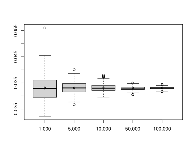
Figure 1: Boot strapping for $\textup{\rm CoCVaR}_{{\eta},{\zeta}}\left({{R_{p}(w)}|{R_{0}}}\right)$. The x-axis is the sample size. Box plots for 100 MCS prices are presented on the plate for each sample size.

We obtain $\textup{\rm CoCVaR}_{{\eta},{\zeta}}\left({{R_{p}(w)}|{R_{0}}}\right)$ as

$$-\mu_{p}(w)-\frac{\sigma_{p}(w)}{\zeta\eta M}\sum_{m=1}^{M}\left(\beta_{p}(w)({\mathcal{T}}_{m}-1)+\epsilon_{p,m}\gamma_{p}(w)\sqrt{{\mathcal{T}}_{m}}\right)1_{\epsilon_{p,m}<C(w,{\mathcal{T}}_{m})}1_{\epsilon_{0}<v({\mathcal{T}}_{m})}$$ (19)

for $(\epsilon_{0,m},\epsilon_{p,m})\in S_{p}$ and ${\mathcal{T}}_{m}\in T$, by MCS and (10). We check the convergence of MCS using bootstrapping. We draw the first boxplot from the left by repeating the MCS 100 times using (19) for a given sample size $M=1000$ in Figure 1. In addition, we draw the other boxplots for each sample size $M\in\{5000,10000,50000,100000\}$, which are presented sequentially after the first box plot in the figure. We also show (by the symbol ‘*’) the CoCVaR computed by numerical integration based on (11). We observe that, as the sample size increases, the interquartile distance of MCS CoCVaR narrows, and dispersions are reduced. All box plots contain the CoCVaR computed by the numerical integration in the interquartile range. The multiple-integral form (11) takes a relatively longer numerical calculation time of 18.13 seconds, while the MCS takes 7.57 seconds for a 100,000 sample size.

Using the same arguments, we can calculate MCT-CoVaR and MCT-CoCVaR using MCS. We calculate the expectations in equations in Proposition 4.2 and 4.3 use the random numbers in $S_{p}$, and $T$, and substitute those MCS expectations into (14), (15), and (16) to obtain $\frac{\partial}{\partial w_{j}}\textup{\rm CoVaR}_{{\eta},{\zeta}}\left({{\Xi_{p}(w)}|{\Xi_{0}}}\right)$ and $\frac{\partial}{\partial w_{j}}\textup{\rm CoCVaR}_{{\eta},{\zeta}}\left({{\Xi_{p}(w)}|{\Xi_{0}}}\right)$. Finally, we obtain $\frac{\partial}{\partial w_{j}}\textup{\rm CoVaR}_{{\eta},{\zeta}}\left({{R_{p}(w)}|{R_{0}}}\right)$ and $\frac{\partial}{\partial w_{j}}\textup{\rm CoCVaR}_{{\eta},{\zeta}}\left({{R_{p}(w)}|{R_{0}}}\right)$ by substituting $\frac{\partial}{\partial w_{j}}\textup{\rm CoVaR}_{{\eta},{\zeta}}\left({{\Xi_{p}(w)}|{\Xi_{0}}}\right)$ and $\frac{\partial}{\partial w_{j}}\textup{\rm CoCVaR}_{{\eta},{\zeta}}\left({{\Xi_{p}(w)}|{\Xi_{0}}}\right)$ into (17), and (18), respectively.

The result of MCT-CoVaR and MCT-CoCVaR values using MCS for each individual stocks of the equally weighted portfolio $R_{p}(w)$ are exhibited in Table 2 with the rank of the values for the ascending order. For example, MCT-CoVaR and MCT-CoCVaR values for MRK rank 1st and those values of AXP rank 30th, respectively. DD ranks 2nd for MCT-CoVaR but 4th for MCT-CoCVaR and so on. We can see that AXP is largest CoVaR and CoCVaR contributor, and is recommended to reduce the proportion of the capital allocation. This idea will be discussed in the Risk Budgeting, below.

5.2 Portfolio Optimization

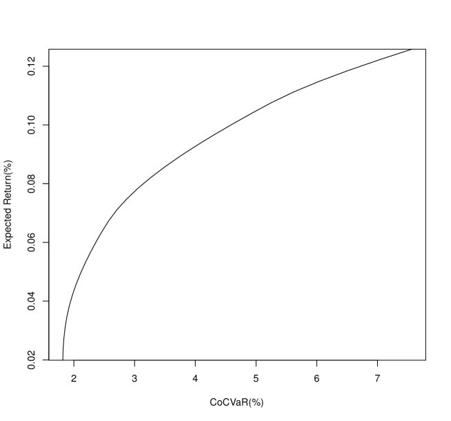
Figure 2: Efficient frontier

Since CoVaR and CoCVaR can capture the relative tail risk under the condition of distressed condition of a benchmark asset or index, we can use those two risk measures for relative portfolio optimization. In this section, we show an empirical example of CoCVaR minimizing portfolio optimization for the 30 stocks with respect to the DJIA index on the NTS market model.

We set a nonlinear programming problem for the portfolio optimization as

$$\min_{w}\textup{\rm CoCVaR}_{{\eta},{\zeta}}\left({{R_{p}(w)}|{R_{0}}}\right)$$

subject to $$w^{\texttt{T}}\mu\geq\mu^{*}$$

$$\sum_{n=1}^{N}w_{n}=1$$

$$w_{n}\geq 0\text{ for all }n\in\{1,2,\cdots,N\}$$

where the benchmark values for the portfolio expected return is $\mu^{*}\in[\min(\mu),\max(\mu)]$. Using the parameters in Table 2, we perform the portfolio optimization for 51 points of $\mu^{*}$ in $\{\mu=\min(\mu)+k\cdot(\max(\mu)-\min(\mu))/50\,|\,k=0,1,2,\cdots,50\}$. We finally obtain the efficient frontier in Figure 2.

Symbol	$\mu_{n}(\%)$	$\sigma_{n}(\%)$	$\beta_{n}(\%)$	KS
DJIA	0.0310	1.4575	$-$3.7939	0.0100	MCT-CoVaR(%)	Rank	MCT-CoCVaR(%)	Rank
AAPL	0.1258	2.1977	$-$1.2679	0.0587	1.6529	17	3.5957	19
AMGN	0.0490	1.6810	1.8704	0.0416	3.2980	22	2.1241	7
AXP	0.0395	2.5245	0.5258	0.0241	7.4288	30	6.6507	30
BA	$-$0.0564	3.4757	3.7589	0.0168	1.7783	18	6.3659	29
CAT	0.0733	2.1609	0.3824	0.0502	5.5670	26	4.8958	22
CRM	0.0284	2.5370	$-$1.0588	0.0514	5.1597	23	5.3903	27
CSCO	0.0117	1.9311	$-$1.3543	0.0323	1.5658	15	2.2187	8
CVX	0.0678	2.4216	1.5941	0.0176	5.6102	27	4.9429	23
DD	$-$0.0096	2.4072	0.3164	0.0593	$-$0.1376	2	1.4762	4
DIS	$-$0.0140	2.1879	4.1225	0.0337	0.3701	10	3.4376	18
GS	0.0791	2.2039	2.0020	0.0485	6.0133	29	5.4714	28
HD	0.0709	1.9351	$-$3.9629	0.0261	5.3208	25	4.9610	24
HON	0.0483	1.8365	$-$2.3242	0.0341	1.5242	14	2.6857	13
IBM	0.0437	1.8054	$-$1.5555	0.0287	0.5364	11	3.1157	16
INTC	$-$0.0314	2.4868	$-$2.8086	0.0295	0.2124	8	2.6130	11
JNJ	0.0260	1.3628	$-$0.5663	0.0285	0.8420	12	1.5451	5
JPM	0.0333	2.1622	2.5850	0.0357	5.6910	28	5.1918	26
KO	0.0324	1.4671	$-$3.6931	0.0249	0.3419	9	2.6197	12
MCD	0.0476	1.5731	1.2955	0.0162	0.2091	7	2.3540	9
MMM	$-$0.0286	1.7824	$-$2.1382	0.0420	0.0681	6	2.7091	14
MRK	0.0461	1.5310	$-$0.0218	0.0463	$-$0.7418	1	0.2360	1
MSFT	0.0879	2.0241	$-$2.1377	0.0469	2.4863	20	3.9390	20
NKE	0.0424	2.1704	$-$0.2999	0.0418	2.4980	21	4.5851	21
PG	0.0511	1.4348	$-$3.0200	0.0322	$-$0.1305	3	0.7501	3
TRV	0.0444	1.9422	$-$2.8043	0.0255	1.1151	13	3.3984	17
UNH	0.0714	1.9919	1.6187	0.0288	0.0165	5	2.5646	10
V	0.0472	1.9411	$-$2.5133	0.0423	5.2771	24	5.1686	25
VZ	$-$0.0226	1.2645	$-$2.5648	0.0357	$-$0.1084	4	0.3166	2
WBA	$-$0.0539	2.2096	$-$1.4927	0.0360	1.6265	16	2.7307	15
WMT	0.0508	1.4940	1.0659	0.0263	2.4613	19	1.7390	6

Table 2: NTS parameter fit using 1-day-returns from 11/27/2018 to 11/15/2022. $\alpha=1.1835$, $\theta=0.0820$

5.3 Risk Budgeting

The MCT-CoVaR and MCT-CoCVaR allow portfolio managers to decide to rebalance their capital allocation weights. Managers can reduce portfolio risk by decreasing the weight of high-risk contributors and increasing the weight of low-risk contributors. The high-risk contributors are assets having high MCT-CoVaR (or MCT-CoCVaR), while the low-risk contributors are assets having low MCT-CoVaR (or MCT-CoCVaR).

Consider a capital allocation vector $w$ for a portfolio with $N$ member stocks. Let $\varDelta w=(\varDelta w_{1}$, $\varDelta w_{2}$, $\cdots$, $\varDelta w_{N})^{\texttt{T}}\in D$ where $D$ is a zero neighborhood in $\mathbb{R}^{N}$, and let

$$\varDelta\textup{\rm CoVaR}_{{\eta},{\zeta}}\left({{R_{P}(w)}|{R_{0}}}\right)=\textup{\rm CoVaR}_{{\eta},{\zeta}}\left({{R_{P}(w+\varDelta w)}|{R_{0}}}\right)-\textup{\rm CoVaR}_{{\eta},{\zeta}}\left({{R_{P}(w)}|{R_{0}}}\right),$$

and

$$\varDelta\textup{\rm CoCVaR}_{{\eta},{\zeta}}\left({{R_{P}(w)}|{R_{0}}}\right)=\textup{\rm CoCVaR}_{{\eta},{\zeta}}\left({{R_{P}(w+\varDelta w)}|{R_{0}}}\right)-\textup{\rm CoCVaR}_{{\eta},{\zeta}}\left({{R_{P}(w)}|{R_{0}}}\right).$$

The optimal portfolios with respect to CoVaR and CoCVaR are obtained by solving the following problem:

$$\min_{\varDelta w}\varDelta\textup{\rm CoVaR}_{{\eta},{\zeta}}\left({{R_{P}(w)}|{R_{0}}}\right)$$ (20)

$$\text{subject to }E[R_{p}(w+\varDelta w)]-E[R_{P}(w)]\geq 0\text{ and }\sum_{j=1}^{N}\varDelta w_{j}=0,$$

and

$$\min_{\varDelta w}\varDelta\textup{\rm CoCVaR}_{{\eta},{\zeta}}\left({{R_{P}(w)}|{R_{0}}}\right)$$ (21)

$$\text{subject to }E[R_{p}(w+\varDelta w)]-E[R_{P}(w)]\geq 0\text{ and }\sum_{j=1}^{N}\varDelta w_{j}=0.$$

Since we have

$$\varDelta\textup{\rm CoVaR}_{{\eta},{\zeta}}\left({{R_{P}(w)}|{R_{0}}}\right)\approx\sum_{j=1}^{N}\left(\frac{\partial}{\partial w_{j}}\textup{\rm CoVaR}_{{\eta},{\zeta}}\left({{R_{P}(w)}|{R_{0}}}\right)\right)\varDelta w_{j},$$

$$\varDelta\textup{\rm CoCVaR}_{{\eta},{\zeta}}\left({{R_{P}(w)}|{R_{0}}}\right)\approx\sum_{j=1}^{N}\left(\frac{\partial}{\partial w_{j}}\textup{\rm CoCVaR}_{{\eta},{\zeta}}\left({{R_{P}(w)}|{R_{0}}}\right)\right)\varDelta w_{j}$$

$$\text{ and }E[R_{p}(w+\varDelta w)]-E[R_{P}(w)]=\sum_{j=1}^{N}\mu_{j}\varDelta w_{j},$$

we can find the optimal portfolio on the local domain $D$ with respect to CoVaR and CoCVaR, respectively, as follows:

$$\varDelta w^{*}=\operatorname*{arg\,min}_{\varDelta w}\sum_{j=1}^{N}\left(\frac{\partial}{\partial w_{j}}\textup{\rm CoVaR}_{{\eta},{\zeta}}\left({{R_{P}(w)}|{R_{0}}}\right)\right)\varDelta w_{j}$$ (22)

$$\text{subject to }\sum_{j=1}^{N}\mu_{j}\varDelta w_{j}\geq 0\text{ and }\sum_{j=1}^{N}\varDelta w_{j}=0.$$

and

$$\varDelta w^{*}=\operatorname*{arg\,min}_{\varDelta w}\sum_{j=1}^{N}\left(\frac{\partial}{\partial w_{j}}\textup{\rm CoCVaR}_{{\eta},{\zeta}}\left({{R_{P}(w)}|{R_{0}}}\right)\right)\varDelta w_{j}$$ (23)

$$\text{subject to }\sum_{j=1}^{N}\mu_{j}\varDelta w_{j}\geq 0\text{ and }\sum_{j=1}^{N}\varDelta w_{j}=0.$$

We perform the risk budgeting for CoVaR and CoCVaR using the 30 stocks in Table 1, i.e. $N=30$, with the estimated parameters in Table 2, iteratively, as the following algorithm:

1. Step 1. Generate a set of independent pairs of standard normal random numbers $S_{0}$, and a set of tempered stable subordinators, $T$, which are independent of $S_{0}$, as we discussed in Section 5.1. Here, the sample size is $M=100,000$.

2. Step 2. Select an initial capital allocation weight vector $w$.

3. Step 3. Find $\mu_{p}(w)$, $\sigma_{p}(w)$, $\beta_{p}(w)$, and $\rho_{p}(w)$ by Proposition 4.1.

4. Step 4. Regenerate a set of bivariate standard normal random vectors $S_{p}=\{(\epsilon_{0,m},\epsilon_{p,m})|\epsilon_{p,m}=\rho_{p}(w)\epsilon_{0,m}+\sqrt{1-(\rho_{p}(w))^{2}}\epsilon_{1,m},(\epsilon_{0,m},\epsilon_{1,m})\in S_{0}\}$ with correlation $\rho_{p}(w)$.

5. Step 5. Calculate MCT-CoVaR or MCT-CoCVaR for $w$ using the MCS method we discussed in Section 5.1.

6. Step 6. Perform risk budgeting and find $\varDelta w^{*}$ using (22), or using (23), for for the CoVaR risk budgeting, or the CoCVaR risk budgeting, respectively.

7. Step 7. Change $w$ to $w+\varDelta w^{*}$ and go to Step 3. Repeat [Step 2 - Step 7] $L$ times.

Let the initial capital allocation weight vector be equally weighted. We perform the iterative risk budgeting $L=200$ times for the local domain be

$$D=\{(x_{1},x_{2},\cdots,x_{30})\,|\,x_{j}\in[-4\cdot 10^{-4},4\cdot 10^{-4}],\,j=1,2,\cdots,30\}.$$

The results are exhibited in Figure 3. For each iteration, we show the values of CoVaR, and CoCVaR with the MCS method in the left and right plate, respectively. The figure shows that the portfolio CoVaR and CoCVaR with respect to the DJIA index decreases as increasing the number of iterations. That is using risk budgeting of CoVaR and CoCVaR on the NTS market model, we obtain a portfolio having the same expected return but less relative tail risk.

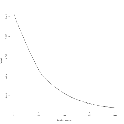
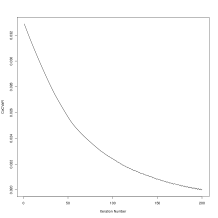
Figure 3: Risk Budgeting iteration

6 conclusion

This paper presents portfolio CoVaR and portfolio CoCVaR on the NTS market model. We develop an MCS method to calculate portfolio CoVaR and CoCVaR, and apply it to portfolio optimization. As an empirical illustration, we consider a portfolio consisting of 30 stocks and measure the CoCVaR of the portfolio with respect to the DJIA index, and then find the efficient frontiers of the portfolio, maximizing the portfolio’s expected return and minimizing the relative tail risk captured by the CoCVaR. In addition, we find an analytic formula for the marginal contributions to CoVaR and CoCVaR, which we calculate using the MCS method to overcome numerical difficulties. We also perform portfolio risk budgeting methods using the marginal contributions to CoVaR and CoCVaR on the NTS market model. We empirically show that the portfolio CoVaR and CoCVaR are decreased by using portfolio budgeting iteratively.

7 Appendix

Proof of Proposition 4.1.

By Proposition 3.1, the stock portfolio return $R_{p}(w)=\sum_{n=1}^{N}w_{n}R_{n}$ is equal to

$$R_{p}(w)=\mu_{p}(w)+\sigma_{p}(w)\Xi_{p}(w),\text{ with }\Xi_{p}(w)\sim\textup{stdNTS}_{1}(\alpha,\theta,\beta_{p}(w),1),$$

where

$$\mu_{p}(w)=\sum_{n=1}^{N}w_{n}\mu_{n},~{}~{}~{}\beta_{p}(w)=\frac{1}{\sigma_{p}(w)}\sum_{n=1}^{N}w_{n}\sigma_{n}\beta_{n}.$$

and

$$\sigma_{p}(w)=\sqrt{\sum_{n=1}^{N}\sum_{m=1}^{N}w_{n}w_{m}\sigma_{n}\sigma_{m}\textrm{\rm cov}\left(\Xi_{n},\Xi_{m}\right)}.$$ (24)

Since $\Xi_{p}(w)=\frac{1}{\sigma_{p}(w)}\sum_{n=1}^{N}w_{n}\sigma_{n}\Xi_{n},$ we have

$$\Xi_{p}(w) =\frac{1}{\sigma_{p}(w)}\sum_{n=1}^{N}\left(w_{n}\sigma_{n}\beta_{n}\left({\mathcal{T}}-1\right)+\gamma_{n}\sqrt{{\mathcal{T}}}\varepsilon_{n}\right)$$

$$=\beta_{p}(w)\left({\mathcal{T}}-1\right)+\frac{\sum_{n=1}^{N}w_{n}\sigma_{n}\gamma_{n}\varepsilon_{n}}{\sigma_{p}(w)}\sqrt{{\mathcal{T}}}$$

with $\gamma_{n}=\sqrt{1-\beta_{n}^{2}\left(\frac{2-\alpha}{2\theta}\right)}$. Note that we have

$$E\left[\frac{\sum_{n=1}^{N}w_{n}\sigma_{n}\gamma_{n}\varepsilon_{n}}{\sigma_{p}(w)}\right]=0$$

and

$$\textrm{\rm var}\left(\frac{\sum_{n=1}^{N}w_{n}\sigma_{n}\gamma_{n}\varepsilon_{n}}{\sigma_{p}(w)}\right) =\frac{1}{\sigma_{p}(w)}\sum_{n=1}^{N}\sum_{m=1}^{N}w_{n}w_{m}\sigma_{n}\sigma_{m}\gamma_{n}\gamma_{n}\rho_{n,m}.$$

By (4) and (24), we get

$$\textrm{\rm var}\left(\frac{\sum_{n=1}^{N}w_{n}\sigma_{n}\gamma_{n}\varepsilon_{n}}{\sigma_{p}(w)}\right) =\frac{1}{(\sigma_{p}(w))^{2}}\sum_{n=1}^{N}\sum_{m=1}^{N}w_{n}w_{m}\sigma_{n}\sigma_{m}\left(\textrm{\rm cov}(\Xi_{n},\Xi_{m})-\beta_{n}\beta_{m}\left(\frac{2-\alpha}{2\theta}\right)\right)$$

$$=1-\frac{1}{(\sigma_{p}(w))^{2}}\left(\sum_{n=1}^{n}w_{n}\sigma_{n}\beta_{n}\right)^{2}\left(\frac{2-\alpha}{2\theta}\right)$$

$$=1-\left(\beta_{p}(w)\right)^{2}\left(\frac{2-\alpha}{2\theta}\right)$$

For the Gaussian property, we get

$$\frac{\sum_{n=1}^{N}w_{n}\sigma_{n}\gamma_{n}\varepsilon_{n}}{\sigma_{p}(w)}=\sqrt{\textrm{\rm var}\left(\frac{\sum_{n=1}^{N}w_{n}\sigma_{n}\gamma_{n}\varepsilon_{n}}{\sigma_{p}(w)}\right)}\varepsilon_{p}=\sqrt{1-\left(\beta_{p}(w)\right)^{2}\left(\frac{2-\alpha}{2\theta}\right)}\varepsilon_{p},$$

where $\varepsilon_{p}\sim\Phi(0,1)$. Hence, we have

$$\Xi_{p}(w)=\beta_{p}(w)\left({\mathcal{T}}-1\right)+\gamma_{p}(w)\sqrt{{\mathcal{T}}}\varepsilon_{p}$$

where $\gamma_{p}(w)=\sqrt{1-\left(\beta_{p}(w)\right)^{2}\left(\frac{2-\alpha}{2\theta}\right)}$. Therefore, we have

$$\textrm{\rm cov}\left(\Xi_{0},\Xi_{p}(w)\right)=\gamma_{0}\gamma_{p}(w)\rho_{0,p}+\beta_{0}\beta_{p}(w)\left(\frac{2-\alpha}{2\theta}\right).$$ (25)

On the other hand, we have

$$\textrm{\rm cov}\left(\Xi_{0},\Xi_{p}(w)\right) =\textrm{\rm cov}\left(\beta_{0}({\mathcal{T}}-1)+\gamma_{0}\sqrt{{\mathcal{T}}}\varepsilon_{0},\frac{1}{\sigma_{p}(w)}\sum_{n=1}^{N}w_{n}\sigma_{n}\left(\beta_{n}({\mathcal{T}}-1)+\gamma_{n}\sqrt{{\mathcal{T}}}\varepsilon_{n}\right)\right)$$

$$=\frac{1}{\sigma_{p}(w)}\sum_{n=1}^{N}w_{n}\sigma_{n}\textrm{\rm cov}\left(\beta_{0}({\mathcal{T}}-1)+\gamma_{0}\sqrt{{\mathcal{T}}}\varepsilon_{0},\beta_{n}({\mathcal{T}}-1)+\gamma_{n}\sqrt{{\mathcal{T}}}\varepsilon_{n}\right)$$

$$=\frac{1}{\sigma_{p}(w)}\sum_{n=1}^{N}w_{n}\sigma_{n}E\left[\left(\beta_{0}({\mathcal{T}}-1)+\gamma_{0}\sqrt{{\mathcal{T}}}\varepsilon_{0}\right)\left(\beta_{n}({\mathcal{T}}-1)+\gamma_{n}\sqrt{{\mathcal{T}}}\varepsilon_{n}\right)\right].$$

Since we have

$$E\left[\left(\beta_{n}({\mathcal{T}}-1)+\gamma_{n}\sqrt{{\mathcal{T}}}\varepsilon_{n}\right)\left(\beta_{0}({\mathcal{T}}-1)+\gamma_{0}\sqrt{{\mathcal{T}}}\varepsilon_{0}\right)\right]$$

$$=E\left[\beta_{n}\beta_{0}({\mathcal{T}}-1)^{2}\right]+E\left[\gamma_{n}\gamma_{0}{\mathcal{T}}\varepsilon_{n}\varepsilon_{0}\right]$$

$$=\beta_{n}\beta_{0}\textrm{\rm var}({\mathcal{T}})+\gamma_{n}\gamma_{0}\rho_{0,n}=\beta_{n}\beta_{0}\left(\frac{2-\alpha}{2\theta}\right)+\gamma_{n}\gamma_{0}\rho_{0,n},$$

we obtain

$$\textrm{\rm cov}\left(\Xi_{0},\Xi_{p}(w)\right) =\frac{1}{\sigma_{p}(w)}\sum_{n=1}^{N}w_{n}\sigma_{n}\left(\beta_{n}\beta_{0}\left(\frac{2-\alpha}{2\theta}\right)+\gamma_{n}\gamma_{0}\rho_{0,n}\right)$$

$$=\beta_{0}\beta_{p}(w)\left(\frac{2-\alpha}{2\theta}\right)+\frac{\gamma_{0}}{\sigma_{p}(w)}\sum_{n=1}^{N}w_{n}\sigma_{n}\gamma_{n}\rho_{0,n}.$$ (26)

By (25) and (26), we have

$$\gamma_{0}\gamma_{p}(w)\rho_{0,p}+\beta_{0}\beta_{p}(w)\left(\frac{2-\alpha}{2\theta}\right)=\beta_{0}\beta_{p}(w)\left(\frac{2-\alpha}{2\theta}\right)+\frac{\gamma_{0}}{\sigma_{p}(w)}\sum_{n=1}^{N}w_{n}\sigma_{n}\gamma_{n}\rho_{0,n}$$

or

$$\rho_{0,p}=\frac{1}{\sigma_{p}(w)\gamma_{p}(w)}\sum_{n=1}^{N}w_{n}\sigma_{n}\gamma_{n}\rho_{0,n}.$$ (27)

Using the definition $\gamma_{p}(w)=\sqrt{1-\left(\beta_{p}(w)\right)^{2}\left(\frac{2-\alpha}{2\theta}\right)}$, we obtain

$$\sigma_{p}(w)\gamma_{p}(w) =\sqrt{\left(\sigma_{p}(w)\right)^{2}-\left(\sigma_{p}(w)\right)^{2}\left(\beta_{p}(w)\right)^{2}\left(\frac{2-\alpha}{2\theta}\right)}$$

$$=\sqrt{\sum_{n=1}^{N}\sum_{m=1}^{N}w_{n}w_{m}\sigma_{n}\sigma_{m}\textrm{\rm cov}\left(\Xi_{n},\Xi_{m}\right)-\left(\sum_{n=1}^{N}w_{n}\sigma_{n}\beta_{n}\right)^{2}\left(\frac{2-\alpha}{2\theta}\right)}$$

$$=\sqrt{\sum_{n=1}^{N}\sum_{m=1}^{N}w_{n}w_{m}\sigma_{n}\sigma_{m}\gamma_{n}\gamma_{m}\rho_{n,m}}.$$ (28)

By substituting (28) into (27), we obtain (8). ∎

Lemma 7.1.

Based on the setting in Section 4.1, we have
(i)

$$\frac{\partial}{\partial w_{j}}\sigma_{p}(w)=\frac{1}{\sigma_{p}(w)}\sum_{n=1}^{N}w_{n}\sigma_{n}\sigma_{j}\textrm{\rm cov}(\Xi_{n},\Xi_{j})$$ (29)

(ii)

$$\frac{\partial}{\partial w_{j}}\beta_{p}(w)=\frac{\sigma_{j}}{\sigma_{p}(w)}\left(\beta_{j}-\frac{\beta_{p}(w)}{\sigma_{p}(w)}\sum_{n=1}^{N}w_{n}\sigma_{n}\textrm{\rm cov}(\Xi_{n},\Xi_{j})\right)$$ (30)

and

$$\frac{\partial}{\partial w_{j}}\gamma_{p}(w)=-\frac{\beta_{p}(w)\left(\frac{2\theta}{2-\alpha}\right)}{\gamma_{p}(w)}\frac{\partial}{\partial w_{j}}\beta_{p}(w)$$ (31)

(iii)

$$\frac{\partial}{\partial w_{j}}u(x,w,t)$$ (32)

$$=\frac{\sigma_{j}}{\sigma_{p}(w)}\left(\frac{1-t}{\gamma_{p}(w)\sqrt{t}}+\frac{u(x,w,t)\beta_{p}(w)\left(\frac{2\theta}{2-\alpha}\right)}{(\gamma_{p}(w))^{2}}\right)\left(\beta_{j}-\frac{\beta_{p}(w)}{\sigma_{p}(w)}\sum_{n=1}^{N}w_{n}\sigma_{n}\textrm{\rm cov}(\Xi_{n},\Xi_{j})\right)$$

(iv) Let

$$C(w,t)=\frac{-\textup{\rm CoVaR}_{{\eta},{\zeta}}\left({{\Xi_{p}(w)}|{\Xi_{0}}}\right)-\beta_{p}(w)(t-1)}{\gamma_{p}(w)\sqrt{t}}$$

Then

$$\frac{\partial}{\partial w_{j}}C(w,t) =-\frac{1}{t(\gamma_{p}(w))^{2}}\frac{\partial}{\partial w_{j}}\textup{\rm CoVaR}_{{\eta},{\zeta}}\left({{\Xi_{p}(w)}|{\Xi_{0}}}\right)$$ (33)

$$+\frac{\sigma_{j}}{\sigma_{p}(w)}\left(\frac{1-t}{\gamma_{p}(w)\sqrt{t}}+\frac{C(w,t)\beta_{p}(w)\left(\frac{2\theta}{2-\alpha}\right)}{(\gamma_{p}(w))^{2}}\right)\left(\beta_{j}-\frac{\beta_{p}(w)}{\sigma_{p}(w)}\sum_{n=1}^{N}w_{n}\sigma_{n}\textrm{\rm cov}(\Xi_{n},\Xi_{j})\right)$$

(v)

$$\frac{\partial}{\partial w_{j}}\rho_{p}(w)=\gamma_{j}\sigma_{j}\left(\frac{\rho_{0,j}}{\sqrt{w^{\texttt{T}}\Sigma_{\gamma,\sigma}^{*}w}}-\frac{\rho_{p}(w)}{w^{\texttt{T}}\Sigma_{\gamma,\sigma}^{*}w}\sum_{n=1}^{N}w_{n}\gamma_{n}\sigma_{n}\rho_{n,j}\right)$$ (34)

Proof.

(i)

$$\frac{\partial}{\partial w_{j}}\sigma_{p}(w) =\frac{1}{2\sigma_{p}(w)}\sum_{n=1}^{N}2w_{n}\sigma_{n}\sigma_{j}\textrm{\rm cov}(\Xi_{n},\Xi_{j})$$

$$=\frac{1}{\sigma_{p}(w)}\sum_{n=1}^{N}w_{n}\sigma_{n}\sigma_{j}\left(\gamma_{n}\gamma_{j}\rho_{n,j}+\beta_{n}\beta_{j}\left(\frac{2-\alpha}{2\theta}\right)\right)$$

(ii)

$$\frac{\partial}{\partial w_{j}}\beta_{p}(w) =\frac{1}{\left(\sigma_{p}(w)\right)^{2}}\left(\sigma_{j}\beta_{j}\sigma_{p}(w)-\left(\sum_{n=1}^{N}w_{n}\sigma_{n}\beta_{n}\right)\frac{\partial}{\partial w_{j}}\sigma_{p}(w)\right)$$

$$=\frac{1}{\left(\sigma_{p}(w)\right)^{2}}\left(\sigma_{j}\beta_{j}\sigma_{p}(w)-\sigma_{p}(w)\beta_{p}(w)\frac{\partial}{\partial w_{j}}\sigma_{p}(w)\right)$$

$$=\frac{\sigma_{j}}{\sigma_{p}(w)}\left(\beta_{j}-\frac{\beta_{p}(w)}{\sigma_{p}(w)}\sum_{n=1}^{N}w_{n}\sigma_{n}\textrm{\rm cov}(\Xi_{n},\Xi_{j})\right)$$

and

$$\frac{\partial}{\partial w_{j}}\gamma_{p}(w) =\frac{-2\beta_{p}(w)\left(\frac{2\theta}{2-\alpha}\right)}{2\sqrt{1-(\beta_{p}(w))^{2}\left(\frac{2\theta}{2-\alpha}\right)}}\frac{\partial}{\partial w_{j}}\beta_{p}(w)=-\frac{\beta_{p}(w)\left(\frac{2\theta}{2-\alpha}\right)}{\gamma_{p}(w)}\frac{\partial}{\partial w_{j}}\beta_{p}(w)$$

(iii) We have

$$\frac{\partial}{\partial w_{j}}u(x,w,t)$$

$$=\frac{1}{t(\gamma_{p}(w))^{2}}\Bigg{(}\left(-(t-1)\frac{\partial}{\partial w_{j}}\beta_{p}(w)\right)\gamma_{p}(w)\sqrt{t}-(x-(t-1)\beta_{p}(w))\sqrt{t}\frac{\partial}{\partial w_{j}}\gamma_{p}(w)\Bigg{)}$$

$$=\left(\frac{1-t}{\gamma_{p}(w)\sqrt{t}}+\frac{u(x,w,t)\beta_{p}(w)\left(\frac{2\theta}{2-\alpha}\right)}{(\gamma_{p}(w))^{2}}\right)\frac{\partial}{\partial w_{j}}\beta_{p}(w).$$ (35)

We obtain (32), by substituting (30) into the last equation.

(iv) We have

$$\frac{\partial}{\partial w_{j}}C(w,t)$$

$$=\frac{1}{t(\gamma_{p}(w))^{2}}\Bigg{(}\left(-\frac{\partial}{\partial w_{j}}\textup{\rm CoVaR}_{{\eta},{\zeta}}\left({{\Xi_{p}(w)}|{\Xi_{0}}}\right)-(t-1)\frac{\partial}{\partial w_{j}}\beta_{p}(w)\right)\gamma_{p}(w)\sqrt{t}$$

$$-\left(-\textup{\rm CoVaR}_{{\eta},{\zeta}}\left({{\Xi_{p}(w)}|{\Xi_{0}}}\right)-(t-1)\beta_{p}(w)\right)\sqrt{t}\frac{\partial}{\partial w_{j}}\gamma_{p}(w)\Bigg{)}$$

$$=-\frac{1}{t(\gamma_{p}(w))^{2}}\frac{\partial}{\partial w_{j}}\textup{\rm CoVaR}_{{\eta},{\zeta}}\left({{\Xi_{p}(w)}|{\Xi_{0}}}\right)+\left(\frac{1-t}{\gamma_{p}(w)\sqrt{t}}+\frac{C(w,t)\beta_{p}(w)\left(\frac{2\theta}{2-\alpha}\right)}{(\gamma_{p}(w))^{2}}\right)\frac{\partial}{\partial w_{j}}\beta_{p}(w).$$

By substituting $C(w,t)=u(x,w,t)|_{x=-\textup{\rm CoVaR}_{{\eta},{\zeta}}\left({{\Xi_{p}(w)}|{\Xi_{0}}}\right)}$ into (35), we have

$$\frac{\partial}{\partial w_{j}}C(w,t) =-\frac{1}{t(\gamma_{p}(w))^{2}}\frac{\partial}{\partial w_{j}}\textup{\rm CoVaR}_{{\eta},{\zeta}}\left({{\Xi_{p}(w)}|{\Xi_{0}}}\right)+\frac{\partial}{\partial w_{j}}u(x,w,t)\Big{|}_{x=-\textup{\rm CoVaR}_{{\eta},{\zeta}}\left({{\Xi_{p}(w)}|{\Xi_{0}}}\right)}.$$

(v)

$$\frac{\partial}{\partial w_{j}}\rho_{p}(w)$$

$$=\frac{1}{w^{\texttt{T}}\Sigma_{\gamma,\sigma}^{*}w}\left(\gamma_{j}\sigma_{j}\rho_{0,j}\sqrt{w^{\texttt{T}}\Sigma_{\gamma,\sigma}^{*}w}-\frac{w^{\texttt{T}}V_{\gamma,\sigma,\rho}^{*}}{2\sqrt{w^{\texttt{T}}\Sigma_{\gamma,\sigma}^{*}w}}\gamma_{j}\sigma_{j}\sum_{n=1}^{N}2w_{n}\gamma_{n}\sigma_{n}\rho_{n,j}\right)$$

$$=\gamma_{j}\sigma_{j}\left(\frac{\rho_{0,j}}{\sqrt{w^{\texttt{T}}\Sigma_{\gamma,\sigma}^{*}w}}-\frac{\rho_{p}(w)}{w^{\texttt{T}}\Sigma_{\gamma,\sigma}^{*}w}\sum_{n=1}^{N}w_{n}\gamma_{n}\sigma_{n}\rho_{n,j}\right)$$

∎

Lemma 7.2.

Let $f^{\Phi_{2}}_{\rho}$ be the pdf of the bivariate standard normal distribution with covariance $\rho$, then we have

$$\int_{0}^{q}f^{\Phi_{2}}_{\rho}(x,K)dx=\frac{1}{\sqrt{2\pi}}\exp\left(-\frac{K^{2}}{2}\right)F_{\Phi}\left(\frac{q-\rho K}{\sqrt{1-\rho^{2}}}\right).$$ (36)

Moreover, if we put $\rho=\rho_{p}(w)$ and let $w_{j}$ be the $j$-th element of $w\in I^{N}$ then we have

$$\frac{\partial}{\partial w_{j}}f^{\Phi_{2}}_{\rho_{p}(w)}(x_{1},x_{2})$$

$$=\left(\frac{\rho_{p}(w)}{1-(\rho_{p}(w))^{2}}-\frac{\rho_{p}(w)x_{1}^{2}-(1+(\rho_{p}(w))^{2})x_{1}x_{2}+\rho_{p}(w)x_{2}^{2}}{(1-(\rho_{p}(w))^{2})^{2}}\right)f^{\Phi_{2}}_{\rho_{p}(w)}(x_{1},x_{2})\frac{\partial}{\partial w_{j}}\rho_{p}(w)$$ (37)

Proof.

We have

$$f^{\Phi_{2}}_{\rho}(x_{1},x_{2})=\frac{1}{2\pi\sqrt{1-\rho^{2}}}\exp\left(-\frac{x_{1}^{2}-2\rho x_{1}x_{2}+x_{2}^{2}}{2(1-\rho^{2})}\right),$$

and hence we obtain

$$\int_{-\infty}^{q}f^{\Phi_{2}}_{\rho}(x,K)dx$$

$$=\int_{-\infty}^{q}\frac{1}{2\pi\sqrt{1-\rho^{2}}}\exp\left(-\frac{x^{2}-2\rho xK+K^{2}}{2(1-\rho^{2})}\right)dx$$

$$=\int_{-\infty}^{q}\frac{1}{2\pi\sqrt{1-\rho^{2}}}\exp\left(-\frac{(x-\rho K)^{2}}{2(1-\rho^{2})}\right)dx\exp\left(-\frac{K^{2}}{2}\right)$$

$$=\frac{1}{\sqrt{2\pi}}\exp\left(-\frac{K^{2}}{2}\right)F_{\Phi}\left(\frac{q-\rho K}{\sqrt{1-\rho^{2}}}\right)$$

which is (36). Moreover, we have

$$\frac{\partial}{\partial w_{j}}f^{\Phi_{2}}_{\rho_{p}(w)}(x_{1},x_{2})$$

$$=\frac{\partial}{\partial w_{j}}\left(\frac{1}{2\pi\sqrt{1-(\rho_{p}(w))^{2}}}\exp\left(-\frac{x_{1}^{2}-2\rho_{p}(w)x_{1}x_{2}+x_{2}^{2}}{2(1-(\rho_{p}(w))^{2})}\right)\right)$$

$$=\frac{1}{2\pi}\exp\left(-\frac{x_{1}^{2}-2\rho_{p}(w)x_{1}x_{2}+x_{2}^{2}}{2(1-(\rho_{p}(w))^{2})}\right)\frac{\partial}{\partial w_{j}}\frac{1}{\sqrt{1-(\rho_{p}(w))^{2}}}$$

$$+\frac{1}{2\pi\sqrt{1-(\rho_{p}(w))^{2}}}\frac{\partial}{\partial w_{j}}\exp\left(-\frac{x_{1}^{2}-2\rho_{p}(w)x_{1}x_{2}+x_{2}^{2}}{2(1-(\rho_{p}(w))^{2})}\right)$$

$$=\frac{1}{2\pi}\exp\left(-\frac{x_{1}^{2}-2\rho_{p}(w)x_{1}x_{2}+x_{2}^{2}}{2(1-(\rho_{p}(w))^{2})}\right)\left(-\frac{1}{2}\right)\left(1-(\rho_{p}(w))^{2}\right)^{-\frac{3}{2}}(-2\rho_{p}(w))\frac{\partial}{\partial w_{j}}\rho_{p}(w)$$

$$+\frac{1}{2\pi\sqrt{1-(\rho_{p}(w))^{2}}}\exp\left(-\frac{x_{1}^{2}-2\rho_{p}(w)x_{1}x_{2}+x_{2}^{2}}{2(1-(\rho_{p}(w))^{2})}\right)\frac{\partial}{\partial w_{j}}\left(-\frac{x_{1}^{2}-2\rho_{p}(w)x_{1}x_{2}+x_{2}^{2}}{2(1-(\rho_{p}(w))^{2})}\right).$$

Since we have

$$\frac{\partial}{\partial w_{j}}\left(-\frac{x_{1}^{2}-2\rho_{p}(w)x_{1}x_{2}+x_{2}^{2}}{2(1-(\rho_{p}(w))^{2})}\right)$$

$$=\frac{-\left(\left(-2x_{1}x_{2}\right)\left(2(1-(\rho_{p}(w))^{2})\right)-(x_{1}^{2}-2\rho_{p}(w)x_{1}x_{2}+x_{2}^{2})2(-2\rho_{p}(w))\right)}{(2(1-(\rho_{p}(w))^{2}))^{2}}\left(\frac{\partial}{\partial w_{j}}\rho_{p}(w)\right)$$

$$=\frac{-\left(-x_{1}x_{2}+x_{1}x_{2}(\rho_{p}(w))^{2}+\rho_{p}(w)x_{1}^{2}-2(\rho_{p}(w))^{2}x_{1}x_{2}+\rho_{p}(w)x_{2}^{2}\right)}{(1-(\rho_{p}(w))^{2})^{2}}\left(\frac{\partial}{\partial w_{j}}\rho_{p}(w)\right)$$

$$=-\frac{\rho_{p}(w)x_{1}^{2}-(1+(\rho_{p}(w))^{2})x_{1}x_{2}+\rho_{p}(w)x_{2}^{2}}{(1-(\rho_{p}(w))^{2})^{2}}\left(\frac{\partial}{\partial w_{j}}\rho_{p}(w)\right)$$

and

$$\frac{\partial}{\partial w_{j}}f^{\Phi_{2}}_{\rho_{p}(w)}(x_{1},x_{2})$$

$$=\frac{1}{2\pi}\exp\left(-\frac{x_{1}^{2}-2\rho_{p}(w)x_{1}x_{2}+x_{2}^{2}}{2(1-(\rho_{p}(w))^{2})}\right)\left(1-(\rho_{p}(w))^{2}\right)^{-\frac{3}{2}}\rho_{p}(w)\frac{\partial}{\partial w_{j}}\rho_{p}(w)$$

$$-\frac{\rho_{p}(w)x_{1}^{2}-(1+(\rho_{p}(w))^{2})x_{1}x_{2}+\rho_{p}(w)x_{2}^{2}}{2\pi\sqrt{1-(\rho_{p}(w))^{2}}(1-(\rho_{p}(w))^{2})^{2}}\exp\left(-\frac{x_{1}^{2}-2\rho_{p}(w)x_{1}x_{2}+x_{2}^{2}}{2(1-(\rho_{p}(w))^{2})}\right)\frac{\partial}{\partial w_{j}}\rho_{p}(w)$$

$$=\left(\frac{\rho_{p}(w)}{1-(\rho_{p}(w))^{2}}-\frac{\rho_{p}(w)x_{1}^{2}-(1+(\rho_{p}(w))^{2})x_{1}x_{2}+\rho_{p}(w)x_{2}^{2}}{(1-(\rho_{p}(w))^{2})^{2}}\right)f^{\Phi_{2}}_{\rho_{p}(w)}(x_{1},x_{2})\frac{\partial}{\partial w_{j}}\rho_{p}(w)$$

which is (7.2). ∎

Proof of Proposition 4.2.

Since $x=-\textup{\rm CoVaR}_{{\eta},{\zeta}}\left({{\Xi_{p}(w)}|{\Xi_{0}}}\right)$, we get

$$\frac{\partial}{\partial w_{j}}\textup{\rm CoVaR}_{{\eta},{\zeta}}\left({{\Xi_{p}(w)}|{\Xi_{0}}}\right)=-\frac{\partial x}{\partial w_{j}}.$$

By applying implicit differentiation, we have

$$\frac{\partial x}{\partial w_{j}}=-\frac{\frac{\partial}{\partial w_{j}}G(x,w)}{\frac{\partial}{\partial x}G(x,w)},$$

and hence

$$\frac{\partial}{\partial w_{j}}\textup{\rm CoVaR}_{{\eta},{\zeta}}\left({{\Xi_{p}(w)}|{\Xi_{0}}}\right)=\frac{\frac{\partial}{\partial w_{j}}G(x,w)}{\frac{\partial}{\partial x}G(x,w)}\Bigg{|}_{x=-\textup{\rm CoVaR}_{{\eta},{\zeta}}\left({{\Xi_{p}(w)}|{\Xi_{0}}}\right)}.$$

We have

$$\frac{\partial}{\partial w_{j}}G(x,w) =\int_{0}^{\infty}\Bigg{(}\int_{-\infty}^{u(x,w,t)}\int_{-\infty}^{v(t)}\frac{\partial}{\partial w_{j}}f^{\Phi_{2}}_{\rho_{p}(w)}(x_{1},x_{2})dx_{1}dx_{2}$$

$$~{}~{}+\int_{-\infty}^{v(t)}f^{\Phi_{2}}_{\rho_{p}(w)}(x_{1},u(x,w,t))dx_{1}\frac{\partial}{\partial w_{j}}u(x,w,t)\Bigg{)}f_{\mathcal{T}}(t)dt$$

By (36), we have

$$\frac{\partial}{\partial w_{j}}G(x,w)$$

$$=\int_{0}^{\infty}\Bigg{(}\int_{-\infty}^{u(x,w,t)}\int_{-\infty}^{v(t)}\frac{\partial}{\partial w_{j}}f^{\Phi_{2}}_{\rho_{p}(w)}(x_{1},x_{2})dx_{1}dx_{2}$$

$$~{}~{}+\frac{1}{\sqrt{2\pi}}\exp\left(-\frac{\left(u(x,w,t)\right)^{2}}{2}\right)F_{\Phi}\left(\frac{v(t)-\rho_{p}(w)u(x,w,t)}{\sqrt{1-(\rho_{p}(w))^{2}}}\right)\frac{\partial}{\partial w_{j}}u(x,w,t)\Bigg{)}f_{\mathcal{T}}(t)dt$$

Hence, by (7.2), we have

$$\int_{0}^{\infty}\int_{-\infty}^{u(x,w,t)}\int_{-\infty}^{v(t)}\frac{\partial}{\partial w_{j}}f^{\Phi_{2}}_{\rho_{p}(w)}(x_{1},x_{2})dx_{1}dx_{2}f_{\mathcal{T}}(t)dt$$

$$=\left(\frac{\partial}{\partial w_{j}}\rho_{p}(w)\right)\int_{0}^{\infty}\Bigg{(}\int_{-\infty}^{u(x,w,t)}\int_{-\infty}^{v(t)}\frac{\rho_{p}(w)}{1-(\rho_{p}(w))^{2}}f^{\Phi_{2}}_{\rho_{p}(w)}(x_{1},x_{2})dx_{1}dx_{2}$$

$$-\int_{-\infty}^{u(x,w,t)}\int_{-\infty}^{v(t)}\frac{\rho_{p}(w)x_{1}^{2}-(1+(\rho_{p}(w))^{2})x_{1}x_{2}+\rho_{p}(w)x_{2}^{2}}{(1-(\rho_{p}(w))^{2})^{2}}f^{\Phi_{2}}_{\rho_{p}(w)}(x_{1},x_{2})dx_{1}dx_{2}\Bigg{)}f_{\mathcal{T}}(t)dt$$

$$=\left(\frac{\partial}{\partial w_{j}}\rho_{p}(w)\right)\Bigg{(}\frac{\rho_{p}(w)}{1-(\rho_{p}(w))^{2}}F_{(\Xi_{0},\Xi_{p}(w))}(v_{0},x)$$

$$-\int_{0}^{\infty}\int_{-\infty}^{u(x,w,t)}\int_{-\infty}^{v(t)}\frac{\rho_{p}(w)x_{1}^{2}-(1+(\rho_{p}(w))^{2})x_{1}x_{2}+\rho_{p}(w)x_{2}^{2}}{(1-(\rho_{p}(w))^{2})^{2}}f^{\Phi_{2}}_{\rho_{p}(w)}(x_{1},x_{2})dx_{1}dx_{2}f_{\mathcal{T}}(t)dt\Bigg{)}$$

Assume that $(\epsilon_{0},\epsilon_{p})$ is the bivariate standard normal random vector with covariance $\rho_{p}(w)$ and ${\mathcal{T}}$ is the tempered stable subordinator with parameters $(\alpha,\theta)$ independent of $(\epsilon_{0},\epsilon_{p})$. Then we have

$$\int_{0}^{\infty}\int_{-\infty}^{u(x,w,t)}\int_{-\infty}^{v(t)}\frac{\partial}{\partial w_{j}}f^{\Phi_{2}}_{\rho_{p}(w)}(x_{1},x_{2})dx_{1}dx_{2}f_{\mathcal{T}}(t)dt$$

$$=\frac{\rho_{p}(w)}{1-(\rho_{p}(w))^{2}}\left(\frac{\partial}{\partial w_{j}}\rho_{p}(w)\right)F_{(\Xi_{0},\Xi_{p}(w))}\left(v_{0},x\right)$$

$$-\frac{\frac{\partial}{\partial w_{j}}\rho_{p}(w)}{(1-(\rho_{p}(w))^{2})^{2}}E\left[(\rho_{p}(w)\epsilon_{p}^{2}-(1+(\rho_{p}(w))^{2})\epsilon_{p}\epsilon_{0}+\rho_{p}(w)\epsilon_{0}^{2})1_{\epsilon_{p}<u(x,w,{\mathcal{T}})}1_{\epsilon_{0}<v({\mathcal{T}})}\right],$$

and hence

$$\frac{\partial}{\partial w_{j}}G(x,w)$$

$$=\frac{\rho_{p}(w)}{1-(\rho_{p}(w))^{2}}\left(\frac{\partial}{\partial w_{j}}\rho_{p}(w)\right)F_{(\Xi_{0},\Xi_{p}(w))}\left(v_{0},x\right)$$

$$-\frac{\frac{\partial}{\partial w_{j}}\rho_{p}(w)}{(1-(\rho_{p}(w))^{2})^{2}}E\left[(\rho_{p}(w)\epsilon_{p}^{2}-(1+(\rho_{p}(w))^{2})\epsilon_{p}\epsilon_{0}+\rho_{p}(w)\epsilon_{0}^{2})1_{\epsilon_{p}<u(x,w,{\mathcal{T}})}1_{\epsilon_{0}<v({\mathcal{T}})}\right]$$

$$~{}~{}+\frac{1}{\sqrt{2\pi}}E\left[\exp\left(-\frac{\left(u(x,w,{\mathcal{T}})\right)^{2}}{2}\right)F_{\Phi}\left(\frac{v({\mathcal{T}})-\rho_{p}(w)u(x,w,{\mathcal{T}})}{\sqrt{1-(\rho_{p}(w))^{2}}}\right)\frac{\partial}{\partial w_{j}}u(x,w,{\mathcal{T}})\right],$$

which is (15). On the other hand, we have

$$\frac{\partial}{\partial x}G(x,w)$$

$$=\int_{0}^{\infty}\int_{-\infty}^{v(t)}f^{\Phi_{2}}_{\rho_{p}(w)}(x_{1},u(x,w,t))dx_{1}\frac{\partial}{\partial x}u(x,w,t)f_{\mathcal{T}}(t)dt$$

$$=\int_{0}^{\infty}\frac{1}{\sqrt{2\pi}}\exp\left(-\frac{\left(u(x,w,t)\right)^{2}}{2}\right)F_{\Phi}\left(\frac{v(t)-\rho_{p}(w)u(x,w,t)}{\sqrt{1-(\rho_{p}(w))^{2}}}\right)\frac{\partial}{\partial x}u(x,w,t)f_{\mathcal{T}}(t)dt$$

by (36). Since we have

$$\frac{\partial}{\partial x}u(x,w,t)=\frac{1}{\gamma_{p}(w)\sqrt{t}},$$

we obtain

$$\frac{\partial}{\partial x}G(x,w)$$

$$=\int_{0}^{\infty}\frac{1}{\sqrt{2\pi}\gamma_{p}(w)\sqrt{t}}\exp\left(-\frac{\left(u(x,w,t)\right)^{2}}{2}\right)F_{\Phi}\left(\frac{v(t)-\rho_{p}(w)u(x,w,t)}{\sqrt{1-(\rho_{p}(w))^{2}}}\right)f_{\mathcal{T}}(t)dt$$

$$=E\left[\frac{1}{\sqrt{2\pi}\gamma_{p}(w)\sqrt{{\mathcal{T}}}}\exp\left(-\frac{\left(u(x,w,{\mathcal{T}})\right)^{2}}{2}\right)F_{\Phi}\left(\frac{v({\mathcal{T}})-\rho_{p}(w)u(x,w,{\mathcal{T}})}{\sqrt{1-(\rho_{p}(w))^{2}}}\right)\right]$$

which is (14). ∎

Proof of Proposition 4.3.

From (11) and the definition of CoCVaR, We have

$$\textup{\rm CoCVaR}_{{\eta},{\zeta}}\left({{\Xi_{p}(w)}|{\Xi_{0}}}\right)=-\frac{H(w)}{F(w)},$$

where

$$H(w)=\int_{0}^{\infty}\int_{-\infty}^{C(w,t)}\int_{-\infty}^{v(t)}\left(\beta_{p}(w)(t-1)+x_{2}\gamma_{p}(w)\sqrt{t}\right)f^{\Phi_{2}}_{\rho_{p}(w)}(x_{1},x_{2})dx_{1}\,dx_{2}\,f_{\mathcal{T}}(t)dt$$

and

$$F(w)=F_{(\Xi_{0},\Xi_{p}(w))}\left(v_{0},-\textup{\rm CoVaR}_{{\eta},{\zeta}}\left({{\Xi_{p}(w)}|{\Xi_{0}}}\right)\right).$$

Thus, we have

$$\frac{\partial}{\partial w_{j}}\textup{\rm CoCVaR}_{{\eta},{\zeta}}\left({{\Xi_{p}(w)}|{\Xi_{0}}}\right)=-\frac{1}{F(w)}\left(\frac{\partial}{\partial w_{j}}H(w)+\textup{\rm CoCVaR}_{{\eta},{\zeta}}\left({{\Xi_{p}(w)}|{\Xi_{0}}}\right)\frac{\partial}{\partial w_{j}}F(w)\right).$$ (38)

(i) Calculating $\frac{\partial}{\partial w_{j}}H(w)$
We have

$$\frac{\partial}{\partial w_{j}}H(w)$$

$$=\int_{0}^{\infty}\Bigg{(}\int_{-\infty}^{v(t)}\left(\beta_{p}(w)(t-1)+C(w,t)\gamma_{p}(w)\sqrt{t}\right)f^{\Phi_{2}}_{\rho_{p}(w)}(x_{1},C(w,t))dx_{1}\frac{\partial}{\partial w_{j}}C(w,t)$$

$$+\int_{-\infty}^{C(w,t)}\int_{-\infty}^{v(t)}\frac{\partial}{\partial w_{j}}\left(\left(\beta_{p}(w)(t-1)+x_{2}\gamma_{p}(w)\sqrt{t}\right)f^{\Phi_{2}}_{\rho_{p}(w)}(x_{1},x_{2})\right)dx_{1}\,dx_{2}\Bigg{)}f_{\mathcal{T}}(t)dt$$

Let

$$I_{1}=\int_{0}^{\infty}\int_{-\infty}^{v(t)}\left(\beta_{p}(w)(t-1)+C(w,t)\gamma_{p}(w)\sqrt{t}\right)f^{\Phi_{2}}_{\rho_{p}(w)}(x_{1},C(w,t))dx_{1}\frac{\partial}{\partial w_{j}}C(w,t)f_{\mathcal{T}}(t)dt$$

and

$$I_{2}=\int_{0}^{\infty}\int_{-\infty}^{C(w,t)}\int_{-\infty}^{v(t)}\frac{\partial}{\partial w_{j}}\left(\left(\beta_{p}(w)(t-1)+x_{2}\gamma_{p}(w)\sqrt{t}\right)f^{\Phi_{2}}_{\rho_{p}(w)}(x_{1},x_{2})\right)dx_{1}\,dx_{2}f_{\mathcal{T}}(t)dt.$$

Then $\frac{\partial}{\partial w_{j}}H(w)=I_{1}+I_{2}$.

Let’s simplify $I_{1}$. Note that $\beta_{p}(w)(t-1)+C(w,t)\gamma_{p}(w)\sqrt{t}=-\textup{\rm CoVaR}_{{\eta},{\zeta}}\left({{\Xi_{p}(w)}|{\Xi_{0}}}\right)$ by the definition of $C(w,t)$. By (36), we have

$$I_{1} =\int_{0}^{\infty}\frac{-\textup{\rm CoVaR}_{{\eta},{\zeta}}\left({{\Xi_{p}(w)}|{\Xi_{0}}}\right)}{\sqrt{2\pi}}\exp\left(-\frac{\left(C(w,t)\right)^{2}}{2}\right)F_{\Phi}\left(\frac{v(t)-\rho_{p}(w)C(w,t)}{\sqrt{1-(\rho_{p}(w))^{2}}}\right)\frac{\partial}{\partial w_{j}}C(w,{\mathcal{T}})f_{\mathcal{T}}(t)dt$$

$$=\frac{-\textup{\rm CoVaR}_{{\eta},{\zeta}}\left({{\Xi_{p}(w)}|{\Xi_{0}}}\right)}{\sqrt{2\pi}}E\left[\exp\left(-\frac{\left(C(w,{\mathcal{T}})\right)^{2}}{2}\right)F_{\Phi}\left(\frac{v({\mathcal{T}})-\rho_{p}(w)C(w,{\mathcal{T}})}{\sqrt{1-(\rho_{p}(w))^{2}}}\right)\frac{\partial}{\partial w_{j}}C(w,{\mathcal{T}})\right],$$

where ${\mathcal{T}}$ is the tempered stable subordinator with parameters $(\alpha,\theta)$.

Consider the integral $I_{2}$. We have

$$\frac{\partial}{\partial w_{j}}\left(\left(\beta_{p}(w)(t-1)+x_{2}\gamma_{p}(w)\sqrt{t}\right)f^{\Phi_{2}}_{\rho_{p}(w)}(x_{1},x_{2})\right)$$

$$=f^{\Phi_{2}}_{\rho_{p}(w)}(x_{1},x_{2})\frac{\partial}{\partial w_{j}}\left(\beta_{p}(w)(t-1)+x_{2}\gamma_{p}(w)\sqrt{t}\right)$$

$$+\left(\beta_{p}(w)(t-1)+x_{2}\gamma_{p}(w)\sqrt{t}\right)\frac{\partial}{\partial w_{j}}f^{\Phi_{2}}_{\rho_{p}(w)}(x_{1},x_{2})$$

$$=f^{\Phi_{2}}_{\rho_{p}(w)}(x_{1},x_{2})\left((t-1)\frac{\partial}{\partial w_{j}}\beta_{p}(w)+x_{2}\sqrt{t}\frac{\partial}{\partial w_{j}}\gamma_{p}(w)\right)$$

$$+\left(\beta_{p}(w)(t-1)+x_{2}\gamma_{p}(w)\sqrt{t}\right)\frac{\partial}{\partial w_{j}}f^{\Phi_{2}}_{\rho_{p}(w)}(x_{1},x_{2}).$$

By (31) and (7.2), we have

$$\frac{\partial}{\partial w_{j}}\left(\left(\beta_{p}(w)(t-1)+x_{2}\gamma_{p}(w)\sqrt{t}\right)f^{\Phi_{2}}_{\rho_{p}(w)}(x_{1},x_{2})\right)$$

$$=f^{\Phi_{2}}_{\rho_{p}(w)}(x_{1},x_{2})\left((t-1)-\frac{x_{2}\beta_{p}(w)\left(\frac{2\theta}{2-\alpha}\right)\sqrt{t}}{\gamma_{p}(w)}\right)\frac{\partial}{\partial w_{j}}\beta_{p}(w)$$

$$+\left(\beta_{p}(w)(t-1)+x_{2}\gamma_{p}(w)\sqrt{t}\right)$$

$$\times\left(\frac{\rho_{p}(w)}{1-(\rho_{p}(w))^{2}}-\frac{\rho_{p}(w)x_{1}^{2}-(1+(\rho_{p}(w))^{2})x_{1}x_{2}+\rho_{p}(w)x_{2}^{2}}{(1-(\rho_{p}(w))^{2})^{2}}\right)$$

$$\times f^{\Phi_{2}}_{\rho_{p}(w)}(x_{1},x_{2})\frac{\partial}{\partial w_{j}}\rho_{p}(w).$$

Hence, we obtain

$$I_{2} =\int_{0}^{\infty}\int_{-\infty}^{C(w,t)}\int_{-\infty}^{v(t)}\left((t-1)-\frac{x_{2}\beta_{p}(w)\left(\frac{2\theta}{2-\alpha}\right)\sqrt{t}}{\gamma_{p}(w)}\right)f^{\Phi_{2}}_{\rho_{p}(w)}(x_{1},x_{2})\frac{\partial}{\partial w_{j}}\beta_{p}(w)$$

$$+\left(\beta_{p}(w)(t-1)+x_{2}\gamma_{p}(w)\sqrt{t}\right)$$

$$\times\left(\frac{\rho_{p}(w)}{1-(\rho_{p}(w))^{2}}-\frac{\rho_{p}(w)x_{1}^{2}-(1+(\rho_{p}(w))^{2})x_{1}x_{2}+\rho_{p}(w)x_{2}^{2}}{(1-(\rho_{p}(w))^{2})^{2}}\right)\frac{\partial}{\partial w_{j}}\rho_{p}(w)$$

$$\times f^{\Phi_{2}}_{\rho_{p}(w)}(x_{1},x_{2})dx_{1}\,dx_{2}\,f_{\mathcal{T}}(t)dt.$$

Let

$$J_{1}=\int_{0}^{\infty}\int_{-\infty}^{C(w,t)}\int_{-\infty}^{v(t)}\left((t-1)-\frac{x_{2}\beta_{p}(w)\left(\frac{2\theta}{2-\alpha}\right)\sqrt{t}}{\gamma_{p}(w)}\right)f^{\Phi_{2}}_{\rho_{p}(w)}(x_{1},x_{2})f_{\mathcal{T}}(t)dt,$$

$$J_{2}=\int_{0}^{\infty}\int_{-\infty}^{C(w,t)}\int_{-\infty}^{v(t)}\left(\beta_{p}(w)(t-1)+x_{2}\gamma_{p}(w)\sqrt{t}\right)f^{\Phi_{2}}_{\rho_{p}(w)}(x_{1},x_{2})dx_{1}\,dx_{2}\,f_{\mathcal{T}}(t)dt,$$

and

$$J_{3} =\int_{0}^{\infty}\int_{-\infty}^{C(w,t)}\int_{-\infty}^{v(t)}\left(\beta_{p}(w)(t-1)+x_{2}\gamma_{p}(w)\sqrt{t}\right)$$

$$\times\left(\frac{\rho_{p}(w)x_{1}^{2}-(1+(\rho_{p}(w))^{2})x_{1}x_{2}+\rho_{p}(w)x_{2}^{2}}{(1-(\rho_{p}(w))^{2})^{2}}\right)f^{\Phi_{2}}_{\rho_{p}(w)}(x_{1},x_{2})dx_{1}\,dx_{2}\,f_{\mathcal{T}}(t)dt$$

Then we have

$$I_{2}=J_{1}\frac{\partial}{\partial w_{j}}\beta_{p}(w)+\left(\frac{\rho_{p}(w)}{1-(\rho_{p}(w))^{2}}J_{2}-J_{3}\right)\frac{\partial}{\partial w_{j}}\rho_{p}(w).$$

We get $J_{2}=-F(w)\textup{\rm CoCVaR}_{{\eta},{\zeta}}\left({{\Xi_{p}(w)}|{\Xi_{0}}}\right)$ by (11). Assume $(\epsilon_{0},\epsilon_{p})$ is the bivariate standard normal distributed random vector with covariance $\rho_{p}(w)$, and ${\mathcal{T}}$ is the tempered stable subordinator with parameters $(\alpha,\theta)$ independent of $(\epsilon_{0},\epsilon_{p})$. Then

$$J_{1}=E\left[\left(({\mathcal{T}}-1)-\frac{\epsilon_{p}\beta_{p}(w)\left(\frac{2\theta}{2-\alpha}\right)\sqrt{{\mathcal{T}}}}{\gamma_{p}(w)}\right)1_{\epsilon_{p}<C(w,{\mathcal{T}})}1_{\epsilon_{0}<v({\mathcal{T}})}\right]$$

and

$$J_{3}=E\left[\left(\frac{\rho_{p}(w)\epsilon_{0}^{2}-(1+(\rho_{p}(w))^{2})\epsilon_{0}\epsilon_{p}+\rho_{p}(w)\epsilon_{p}^{2}}{(1-(\rho_{p}(w))^{2})^{2}}\right)\xi_{p}(w)1_{\epsilon_{p}<C(w,{\mathcal{T}})}1_{\epsilon_{0}<v({\mathcal{T}})}\right]$$

where $\xi_{p}(w)=\beta_{p}(w)({\mathcal{T}}-1)+\epsilon_{p}\gamma_{p}(w)\sqrt{{\mathcal{T}}}$. Substituting $I_{1}$, $J_{1}$, $J_{2}$, $J_{3}$ into

$$\frac{\partial}{\partial w_{j}}H(w)=I_{1}+J_{1}\frac{\partial}{\partial w_{j}}\beta_{p}(w)+\left(\frac{\rho_{p}(w)}{1-(\rho_{p}(w))^{2}}J_{2}-J_{3}\right)\frac{\partial}{\partial w_{j}}\rho_{p}(w),$$

we obtain

$$\frac{\partial}{\partial w_{j}}H(w)$$ (39)

$$=\frac{-\textup{\rm CoVaR}_{{\eta},{\zeta}}\left({{\Xi_{p}(w)}|{\Xi_{0}}}\right)}{\sqrt{2\pi}}E\left[\exp\left(-\frac{\left(C(w,{\mathcal{T}})\right)^{2}}{2}\right)F_{\Phi}\left(\frac{v({\mathcal{T}})-\rho_{p}(w)C(w,{\mathcal{T}})}{\sqrt{1-(\rho_{p}(w))^{2}}}\right)\frac{\partial}{\partial w_{j}}C(w,{\mathcal{T}})\right]$$

$$+E\left[\left(({\mathcal{T}}-1)-\frac{\epsilon_{p}\beta_{p}(w)\left(\frac{2\theta}{2-\alpha}\right)\sqrt{{\mathcal{T}}}}{\gamma_{p}(w)}\right)1_{\epsilon_{p}<C(w,{\mathcal{T}})}1_{\epsilon_{0}<v({\mathcal{T}})}\right]\frac{\partial}{\partial w_{j}}\beta_{p}(w)$$

$$-\frac{\rho_{p}(w)}{1-(\rho_{p}(w))^{2}}\left(\frac{\partial}{\partial w_{j}}\rho_{p}(w)\right)F(w)\textup{\rm CoCVaR}_{{\eta},{\zeta}}\left({{\Xi_{p}(w)}|{\Xi_{0}}}\right)$$

$$-E\left[\left(\frac{\rho_{p}(w)\epsilon_{0}^{2}-(1+(\rho_{p}(w))^{2})\epsilon_{0}\epsilon_{p}+\rho_{p}(w)\epsilon_{p}^{2}}{(1-(\rho_{p}(w))^{2})^{2}}\right)\xi_{p}(w)1_{\epsilon_{p}<C(w,{\mathcal{T}})}1_{\epsilon_{0}<v({\mathcal{T}})}\right]\frac{\partial}{\partial w_{j}}\rho_{p}(w).$$

(ii) Calculating $\frac{\partial}{\partial w_{j}}F(w)$
Since we have

$$F(w)=\int_{0}^{\infty}\int_{-\infty}^{C(w,t)}\int_{-\infty}^{v(t)}f^{\Phi_{2}}_{\rho_{p}(w)}(x_{1},x_{2})dx_{1}dx_{2}f_{\mathcal{T}}(t)dt,$$

we get

$$\frac{\partial}{\partial w_{j}}F(w) =\int_{0}^{\infty}\Bigg{(}\int_{-\infty}^{C(w,t)}\int_{-\infty}^{v(t)}\frac{\partial}{\partial w_{j}}f^{\Phi_{2}}_{\rho_{p}(w)}(x_{1},x_{2})dx_{1}dx_{2}$$

$$~{}~{}+\int_{-\infty}^{v(t)}f^{\Phi_{2}}_{\rho_{p}(w)}(x_{1},u(x,w,t))dx_{1}\frac{\partial}{\partial w_{j}}C(w,t)\Bigg{)}f_{\mathcal{T}}(t)dt$$

Using the same arguments in the proof of Proposition 4.2, we obtain

$$\frac{\partial}{\partial w_{j}}F(w)$$ (40)

$$=\frac{\rho_{p}(w)}{1-(\rho_{p}(w))^{2}}\left(\frac{\partial}{\partial w_{j}}\rho_{p}(w)\right)F(w)$$

$$-E\left[\left(\frac{\rho_{p}(w)\epsilon_{p}^{2}-(1+(\rho_{p}(w))^{2})\epsilon_{p}\epsilon_{0}+\rho_{p}(w)\epsilon_{0}^{2}}{(1-(\rho_{p}(w))^{2})^{2}}\right)1_{\epsilon_{p}<C(w,{\mathcal{T}})}1_{\epsilon_{0}<v({\mathcal{T}})}\right]\frac{\partial}{\partial w_{j}}\rho_{p}(w)$$

$$~{}~{}+\frac{1}{\sqrt{2\pi}}E\left[\exp\left(-\frac{\left(C(w,{\mathcal{T}})\right)^{2}}{2}\right)F_{\Phi}\left(\frac{v({\mathcal{T}})-\rho_{p}(w)u(x,w,{\mathcal{T}})}{\sqrt{1-(\rho_{p}(w))^{2}}}\right)\frac{\partial}{\partial w_{j}}C(w,{\mathcal{T}})\right].$$

By substituting (39), (40), and $F(w)=F_{(\Xi_{0},\Xi_{p}(w))}\left(v_{0},-\textup{\rm CoVaR}_{{\eta},{\zeta}}\left({{\Xi_{p}(w)}|{\Xi_{0}}}\right)\right)=\eta\zeta$ into (38), we get

$$\frac{\partial}{\partial w_{j}}\textup{\rm CoCVaR}_{{\eta},{\zeta}}\left({{\Xi_{p}(w)}|{\Xi_{0}}}\right)$$

$$= -\frac{1}{\eta\zeta}\Bigg{(}E\left[\left(({\mathcal{T}}-1)-\frac{\epsilon_{p}\beta_{p}(w)\left(\frac{2\theta}{2-\alpha}\right)\sqrt{{\mathcal{T}}}}{\gamma_{p}(w)}\right)1_{\epsilon_{p}<C(w,{\mathcal{T}})}1_{\epsilon_{0}<v({\mathcal{T}})}\right]\frac{\partial}{\partial w_{j}}\beta_{p}(w)$$

$$-E\left[\left(\frac{\rho_{p}(w)\epsilon_{0}^{2}-(1+(\rho_{p}(w))^{2})\epsilon_{0}\epsilon_{p}+\rho_{p}(w)\epsilon_{p}^{2}}{(1-(\rho_{p}(w))^{2})^{2}}\right)\xi_{p}(w)1_{\epsilon_{p}<C(w,{\mathcal{T}})}1_{\epsilon_{0}<v({\mathcal{T}})}\right]\frac{\partial}{\partial w_{j}}\rho_{p}(w)$$

$$-\textup{\rm CoCVaR}_{{\eta},{\zeta}}\left({{\Xi_{p}(w)}|{\Xi_{0}}}\right)E\left[\left(\frac{\rho_{p}(w)\epsilon_{p}^{2}-(1+(\rho_{p}(w))^{2})\epsilon_{p}\epsilon_{0}+\rho_{p}(w)\epsilon_{0}^{2}}{(1-(\rho_{p}(w))^{2})^{2}}\right)1_{\epsilon_{p}<C(w,{\mathcal{T}})}1_{\epsilon_{0}<v({\mathcal{T}})}\right]\frac{\partial}{\partial w_{j}}\rho_{p}(w)\Bigg{)}$$

Hence we obtain (16).

∎

References

- Adrian and Brunnermeier (2016) Adrian, T. and Brunnermeier, M. K. (2016). Covar. American Economic Review, 106(7), 1705–41. URL https://www.aeaweb.org/articles?id=10.1257/aer.20120555.
- Anand et al. (2016) Anand, A., Li, T., Kurosaki, T., and Kim, Y. S. (2016). Foster-Hart optimal portfolios. Journal of Banking and Finance, 68, 117–130.
- Anand et al. (2017) Anand, A., Li, T., Kurosaki, T., and Kim, Y. S. (2017). The equity risk posed by the too-big-to-fail banks: A foster-hart estimation. Annals of Operations Research, 253(1), 21–41.
- Barndorff-Nielsen (1978) Barndorff-Nielsen, O. (1978). Hyperbolic distributions and distributions on hyperbolae. Scandinavian Journal of Statistics, 5(3), 151–157.
- Barndorff-Nielsen and Levendorskii (2001) Barndorff-Nielsen, O. E. and Levendorskii, S. (2001). Feller processes of normal inverse Gaussian type. Quantitative Finance, 1, 318 – 331.
- Barndorff-Nielsen and Shephard (2001) Barndorff-Nielsen, O. E. and Shephard, N. (2001). Normal modified stable processes. Economics Series Working Papers from University of Oxford, Department of Economics, 72.
- Cont and Tankov (2004) Cont, R. and Tankov, P. (2004). Financial Modelling with Jump Processes. Chapman & Hall / CRC.
- Eberlein and Madan (2010) Eberlein, E. and Madan, D. B. (2010). On correlating Lévy processes. Journal of Risk, 13(1), 3–16.
- Fama (1963) Fama, E. (1963). Mandelbrot and the stable Paretian hypothesis. Journal of Business, 36, 420–429.
- Gil-Pelaez (1951) Gil-Pelaez, J. (1951). Note on the inversion theorem. Biometrika, 38(3-4).
- Girardi and Tolga Ergün (2013) Girardi, G. and Tolga Ergün, A. (2013). Systemic risk measurement: Multivariate garch estimation of covar. Journal of Banking & Finance, 37(8), 3169–3180. URL https://www.sciencedirect.com/science/article/pii/S0378426613001155.
- Gourieroux et al. (2000) Gourieroux, C., Laurent, J., and Scaillet, O. (2000). Sensitivity analysis of values at risk. Journal of Empirical Finance, 7, 225–245.
- Huang and Uryasev (2018) Huang, W.-Q. and Uryasev, S. P. (2018). The cocvar approach: systemic risk contribution measurement. Journal of Risk, 20, 75–93.
- Kim (2005) Kim, Y. (2005). The Modified Tempered Stable Processes with Applications to Finance. Ph.D. thesis, Sogang University.
- Kim (2022) Kim, Y. S. (2022). Portfolio optimization and marginal contribution to risk on multivariate normal tempered stable model. Annals of Operations Research, 1–29.
- Kim et al. (2012) Kim, Y. S., Giacometti, R., Rachev, S. T., Fabozzi, F. J., and Mignacca, D. (2012). Measuring financial risk and portfolio optimization with a non-Gaussian multivariate model. Annals of Operations Research, 201(1), 325–343.
- Kim et al. (2023) Kim, Y. S., Kim, H., Choi, J., and Fabozzi, F. J. (2023). Multi-asset option pricing using normal tempered stable processes with stochastic correlation. The Journal of Derivatives, 30(3), 42–64.
- Kim et al. (2015) Kim, Y. S., Lee, J., Mittnik, S., and Park, J. (2015). Quanto option pricing in the presence of fat tails and asymmetric dependence. Journal of Econometrics, 187(2), 512 – 520.
- Kim and Volkmann (2013) Kim, Y. S. and Volkmann, D. (2013). NTS copula and finance. Applied Mathematics Letters, 26, 676–680.
- Kurosaki and Kim (2018) Kurosaki, T. and Kim, Y. S. (2018). Foster-Hart optimization for currency portfolio. Studies in Nonlinear Dynamics & Econometrics, 23(2), Published Online.
- Kurosaki and Kim (2022) Kurosaki, T. and Kim, Y. S. (2022). Cryptocurrency portfolio optimization with multivariate normal tempered stable processes and foster-hart risk. Finance Research Letters, 45, 102143.
- Liu et al. (2021) Liu, Y., Djurić, P. M., Kim, Y. S., Rachev, S. T., and Glimm, J. (2021). Systemic risk modeling with Lévy copulas. Journal of Risk and Financial Management, 14(6), 251.
- Mandelbrot (1963a) Mandelbrot, B. B. (1963a). New methods in statistical economics. Journal of Political Economy, 71, 421–440.
- Mandelbrot (1963b) Mandelbrot, B. B. (1963b). The variation of certain speculative prices. Journal of Business, 36, 394–419.
- Markowitz (1952) Markowitz, H. (1952). Portfolio selection. Journal of Finance, 7(1), 77–91.
- Reboredo and Ugolini (2015) Reboredo, J. C. and Ugolini, A. (2015). Systemic risk in european sovereign debt markets: A covar-copula approach. Journal of International Money and Finance, 51, 214–244. URL https://www.sciencedirect.com/science/article/pii/S0261560614002162.
- Stoyanov et al. (2013) Stoyanov, S. V., Rachev, S. T., and Fabozzi, F. J. (2013). Sensitivity of portfolio VaR and CVaR to portfolio return characteristics. Annals of Operations Research, 205, 169–187.