Baek et al.

Policy Optimization for Personalized Interventions

Policy Optimization for Personalized Interventions in Behavioral Health Jackie BaekNYU Stern School of Business, baek@stern.nyu.edu Justin J. BoutilierDepartment of Industrial and Systems Engineering, University of Wisconsin-Madison, j.boutilier@wisc.edu Vivek F. FariasMIT Sloan School of Management, vivekf@mit.edu Jónas Oddur JónassonMIT Sloan School of Management, joj@mit.edu Erez YoeliMIT Sloan School of Management, eyoeli@mit.edu

Behavioral health interventions, delivered through digital platforms, have the potential to significantly improve health outcomes, through education, motivation, reminders, and outreach. We study the problem of optimizing personalized interventions for patients to maximize a long-term outcome, where interventions are costly and capacity-constrained. We assume there exists a dataset collected from an initial pilot study that we can leverage. We present a new approach for this problem that we dub $\mathsf{DecompPI}$, which approximates one step of policy iteration. Implementing $\mathsf{DecompPI}$ simply consists of a prediction task using the dataset, alleviating the need for online experimentation. $\mathsf{DecompPI}$ is a generic model-free algorithm that can be used irrespective of the underlying patient behavior model. We derive theoretical guarantees on a simple, special case of the model that is representative of our problem setting. We establish an approximation ratio for $\mathsf{DecompPI}$ with respect to the improvement beyond a null policy that does not allocate interventions. Specifically, when the initial policy used to collect the data is randomized, the approximation ratio of the improvement approaches 1/2 as the intervention capacity of the initial policy decreases. We show that this guarantee is robust to estimation errors. We conduct a rigorous empirical case study using real-world data from a mobile health platform for improving treatment adherence for tuberculosis. Using a validated simulation model, we demonstrate that $\mathsf{DecompPI}$ can provide the same efficacy as the status quo approach with approximately half the capacity of interventions. $\mathsf{DecompPI}$ is simple and easy to implement for organizations aiming to improve long-term behavior through targeted interventions, and this paper demonstrates its strong performance both theoretically and empirically.

Health Analytics, Behavioral Health, Policy Optimization, Reinforcement Learning, Tuberculosis, Global Health

1 Introduction

For most health conditions, long-term outcomes are determined not only by clinical interventions but also by individual habits and behaviors (Bosworth et al. 2011). A range of behavioral health interventions, often delivered through digital platforms, have been shown to improve outcomes for various health conditions. These interventions aspire to affect users’ habits through motivation, education, nudging, or boosting (Ruggeri et al. 2020). At the same time, such interventions are associated with a variety of direct and indirect costs. This paper is concerned with optimizing the impact of costly interventions through prioritization.

As a concrete example of a digital health intervention, consider our partner organization, Keheala. Keheala operates a digital service promoting medication adherence among patients prescribed with tuberculosis (TB) treatment in Kenya, and has already been shown to have a non-trivial impact on adherence and health outcomes (Yoeli et al. 2019, Boutilier et al. 2022). Increasing adherence to the prescribed course of treatment for TB is important since lack thereof can result in a relapse of the disease, and worse yet, the emergence of multi-drug resistant strains of the TB bacteria. A key feature of Keheala’s adherence program is that patients are required to self-verify treatment adherence daily via a mobile phone interface. In addition, Keheala’s digital platform comprises of a suite of interventions to further support adherence. Some are on-demand (e.g., leaderboards and information about TB) and some are automated (e.g., daily reminders to adhere to treatment). Most importantly, some are manual (e.g., outreach messages and phone calls). Keheala employs support sponsors to operate the platform and reach out to patients who have not self-verified adherence for a predetermined amount of time. The interactions between the platform and the patients result in a feedback loop that presents an opportunity for Keheala to discern the impact of each type of intervention as well as to identify patients most in need of outreach.

The Keheala case highlights three salient features that are common among digital services in the context of behavioral health services.

1. Interventions are costly and must be rationed. In general, even automated mobile reminders entail an indirect cost, in that frequent reminders are likely to sensitize patients to the automated messages. In the case of Keheala, calls from support sponsors entail a direct cost. Due to these costs, demand for support sponsor outreach exceeds supply. The support sponsors had a range of responsibilities but on an average day in our data (see more details in Section 5) their effective capacity to make phone calls to patients was exceeded by the number of patients eligible for such phone calls by a factor of 8.

2. The short-term metric of interest is a binary measure of compliance among users. For many behavioral health applications, a service provider (e.g., digital platform) collects data from users, aimed at identifying whether they are in a state of compliance with a desired behavior (e.g., medication adherence, exercise routine, correct diet) or not. In the case of Keheala, this binary outcome measure is the daily self-verification of treatment adherence.

3. Initially, limited data is collected using an ad-hoc baseline policy. Most digital behavioral health platforms are initially launched (e.g., as part of a pilot study) with heuristic rules of thumb guiding the timing of outreach to each user (Mills 2020). In Keheala’s case, an RCT was conducted in which the protocol stated that patients who had not self-verified their adherence for 48 hours should be prioritized for support sponsor outreach.

This state of affairs prompts the key question we seek to answer: Can one use limited pilot-study data, collected using some ad-hoc baseline policy, to design a practical intervention policy that maximizes the impact of costly interventions?

1.1 What can Reinforcement Learning Offer?

Before diving into the development of a new approach to the problem, let us explore an out-of-the-box approach for this problem. Natural candidates for personalizing outreach interventions using data are reinforcement learning (RL) algorithms. As a prototype of the sorts of RL approaches that one might apply to intervention optimization, consider formulating the task at hand as a so-called contextual bandit. Specifically, the context of a given patient is their adherence and intervention history so far, and the reward corresponds to whether or not they self-verify treatment adherence in the following day. This reward is assumed to be some unknown, noisy function of context and the chosen action (i.e., whether or not the patient received an intervention). Of course, a myopically optimal action may be sub-optimal, but let us ignore this limitation for now.

Figure 1 compares the performance of a common contextual bandit algorithm, Thompson Sampling, with that of the existing heuristic employed by Keheala using a simulation model fit to data from Keheala’s initial pilot. In parsing this figure, we note that the x-axis corresponds to the number of calls (and thus, also the amount of data that can be collected about the incremental impact of an intervention) in a single day. The operating point for the Keheala pilot corresponds to a budget of 26 interventions per day, as indicated by the yellow star.

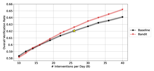
Figure 1: Average overall verification rate over 50 runs for each policy and budget. The shaded region indicates a 95% confidence interval. The star represents the operating point for Keheala.

While we acknowledge that a contextual bandit is only one simple approach to our problem (we will include more sophisticated benchmarks in our numerical analysis in Section 5) it is illustrative to highlight some of its shortcomings, relative to the criteria we had listed above. Setting aside the obvious issue that a contextual bandit relies on online exploration (whereas we would like to learn from offline data), we make three additional observations. First, in general we observe modest improvements. The bandit captures a similar verification rate as the incumbent Keheala policy with 3 fewer interventions per day (relative to the 26 used by Keheala). While meaningful, this is a somewhat marginal improvement. Second, performance can actually deteriorate, relative to the baseline policy, particularly in the most resource-limited cases. As we further discuss in Section 5.5, this is a data scarcity issue: with a small budget, the bandit simply does not collect enough exploration data to learn an improved policy. This is despite the fact that the Thompson sampling algorithm employed had the benefit of a prior learned on approximately half of the data. Third, the contextual bandit is (by design) a myopic approach. In essence, the bandit learns to provide outreach in such a way as to maximize the next day’s self-verification rates, which may be highly suboptimal for the long term. While, we could certainly turn to a reinforcement learning algorithm that attempts to learn an optimal policy by measuring the long run impact of an action, the data requirements of such a policy would increase substantively so that the performance degradation we see for the bandit at low budgets is likely to persist at (much) higher budgets.

In summary, this leaves us in a peculiar spot—whereas more sophisticated RL algorithms could, in principle, learn an optimal policy, we typically do not have the data budget, or the willingness to risk policy degradation due to exploration, to use such approaches. However, simpler RL algorithms (such as the contextual bandit) provide a relatively marginal improvement.

1.2 This Paper

In this paper, we propose and evaluate a new algorithm for intervention optimization problems of the type described above.

Our first contribution is the algorithm itself (Section 3). Our starting point is a formal model of the rich practical setting of interest where we model patient behaviors using a generic Markov Decision Process (MDP)—we refer to this as the ‘full model’. We propose a new approach—inspired by existing techniques—for intervention optimization problems we dub Decomposed Policy Iteration $(\mathsf{DecompPI})$. Loosely, $\mathsf{DecompPI}$ can be thought of as approximating a single step of policy iteration in the high dimensional MDP corresponding to our problem. Taking as input a dataset of interventions and outcomes under an incumbent policy, we estimate the state-action values ($q$-values) of this policy using a prediction algorithm. Then, at each time step, interventions are assigned to the patients who have the largest increase in their $q$-value if they receive an intervention, compared to if they do not. Notably, the $q$-values are decomposed at the patient level, which avoids any dependence on an exponentially sized state space. $\mathsf{DecompPI}$ is a promising practical solution to intervention optimization problems as it is model-free (i.e., does not require access to a model of the environment) and hence it does not rely on positing a particular behavioral model. It also does not rely on online experimentation or updating, as is the case for many RL algorithms.

Our second contribution is to provide surprisingly strong performance guarantees for $\mathsf{DecompPI}$ when applied to a stylized version of the full problem (Section 4). In general, a single step of policy iteration does not provide a meaningful performance guarantee. However, patient dynamics with respect to habitual behavior are not arbitrary. We therefore study the performance of our algorithm when patient behavior is driven by a standard simple model akin to models considered both in the behavioral health (Mate et al. 2020, 2022, Biswas et al. 2021) and marketing literature (Schmittlein et al. 1987). For situations in which user behavior is driven by such models, we establish an approximation ratio of the improvement between an optimal policy and a null policy that does not allocate interventions. Notably, this result is much stronger than a typical approximation guarantee, which compares the absolute performance of a policy to the optimal policy. Specifically, when the baseline policy used to the collect the data is randomized, the approximation ratio of the improvement approaches $1/2$ as the intervention capacity decreases. Since the quantities used by $\mathsf{DecompPI}$ need to be estimated, we prove that our guarantee is robust in the sense that the performance guarantee scales gracefully with respect to errors in these quantities.

Our third contribution is to return to the full model and provide numerical results based on field data (Section 5). Using the validated simulation setup described in Figure 1, we find that $\mathsf{DecompPI}$ would yield the same verification rate as the incumbent Keheala policy with less than half the capacity. Furthermore, $\mathsf{DecompPI}$ outperforms the contextual bandit algorithm (described above) for budgets ranging from 50% to 150% of the original capacity. Importantly, the performance gains are highest in low capacity scenarios—the most likely paradigm for a future large-scale roll-out of the system in resource-limited settings. This is encouraging for digital behavioral health applications, more generally—particularly given how well the policy performs despite only having access to limited data collected during pilot implementation.

2 Literature Review

Our work relates to the expansive streams of literature on reinforcement learning and (approximate) dynamic programming, as well as the applied operations research literature focusing on improving healthcare delivery in resource-limited settings. Methodologically speaking, most existing solution approaches to problems similar to ours can be classified as either (a) developing policies for a known underlying model of behavior or (b) learning a policy using data. We summarize these two streams of work in Sections 2.1 and 2.2, respectively, before discussing prior work on TB treatment as an application area in Section 2.3.

2.1 Known Model

Our model (described in detail in Section 3.1) assumes that every patient behaves according to a Markov decision process (MDP). Even if all the MDP parameters of these models were known exactly, the size of the system state space would be exponential in the number of patients: the size of the state space is $|\mathcal{S}|^{N}$, where $\mathcal{S}$ is the state space for one patient and $N$ is the number of patients. As a result, a direct application of dynamic programming techniques such as backwards induction or policy/value iteration would take exponential time and hence is practically infeasible.

As exact methods are infeasible, one can resort to approximate dynamic programming (ADP) techniques developed for weakly-coupled MDPs (e.g., Meuleau et al. 1998, Adelman and Mersereau 2008, D’Aeth et al. 2023). Specifically, the model we study is a restless bandit: each patient corresponds to an arm, there is a budget on the number of arms that can be ‘pulled’ (given an intervention) at each time step. The state of each arm evolves as a Markov chain, where its transition probabilities depend on the action taken. It is known that finding the optimal policy to a restless bandit is PSPACE-hard (Papadimitriou and Tsitsiklis 1994). There is a large literature on developing algorithms for this problem (e.g., Whittle 1988, Glazebrook and Mitchell 2002, Ansell et al. 2003, Glazebrook et al. 2006, Liu and Zhao 2010, Guha et al. 2010). A commonly used policy is the Whittle’s index (Whittle 1988), which is known to be asymptotically optimal under certain conditions (Weber and Weiss 1990) and has been shown to have good empirical performance (Ansell et al. 2003, Glazebrook and Mitchell 2002, Glazebrook et al. 2006). All of the above methods assume that the model is known, whereas our problem has the further nontrivial complication that the model is unknown.

2.2 Unknown Model

Deriving an optimal policy for an MDP with unknown parameters is corresponds to reinforcement learning (RL), a rapidly expanding area of research (Sutton and Barto 2018). However, a naive application of the RL framework onto our problem results in an exponentially large state space — this correspondingly results in an exponential blowup in the data requirements to deploy generic RL methods such as Q-learning (Jin et al. 2018). Therefore, more tailored approaches are required to fit to this regime.

Greedy and multi-armed bandits.

One approach, as described in the introduction, is to greedily maximize the immediate reward at each time step. For example, in the treatment adherence setting, one can reach out to patients with the highest increase in their probability of adhering in the next day from the intervention. A multi-armed bandit is one natural framework that can be used to learn such a policy. This is the approach used in HeartSteps (Lei et al. 2017, Liao et al. 2020), a program to promote physical activity using real-time data collected from wristband sensors. These papers use a contextual bandit model, where the context represents a user at a particular time step, and they develop a bandit algorithm whose goal is to increase the immediate activity level of the user. Given the vast literature on contextual bandits, there are a wide variety of algorithms that one can easily plug in.

A fundamental downside of this greedy approach is that it does not capture any potential long-term effects of an action—that is, an action may not only impact a patient’s immediate behavior, but their behavior for all future time steps. One way to address this is to specifically model the type of long-term effect it can have. For example, Liao et al. (2020) introduce a ‘dosage’ variable that models the phenomenon that the treatment effect of an action is often smaller when an action was recently given to that patient in the past. Similarly, Mintz et al. (2020) incorporate habituation and recovery dynamics into the bandit framework. However, these approaches captures only particular types of long-term effects that are explicitly modeled, and there could be other, complex factors that affect the downstream behavior of patients.

Our work does not take this greedy approach, and we aim to learn a policy that maximizes long-term rewards, without specifically modeling the type of long-term effect that an action can have. We benchmark against a contextual bandit policy, and we observe that incorporating the long-term effects is critical in the behavioral health setting that we study.

Learning for restless bandits.

A non-greedy approach to this problem corresponds to the restless bandit model in the unknown parameter regime. There is a nascent literature develops learning algorithms in this setting. One approach is to adapt algorithms from the multi-armed bandit literature such as UCB (Wang et al. 2020b) or Thompson Sampling (Jung and Tewari 2019). Recent approaches similarly adapt reinforcement learning methods such as Q-learning (e.g., Fu et al. 2019, Avrachenkov and Borkar 2022). Importantly, these methods are online learning algorithms that require continuous exploration and assume that the state space is known and finite. This literature focuses on providing theoretical guarantees of the proposed algorithms eventually converging to the optimal policy.

Our work differs from the aforementioned literature in a couple of ways. First, we take an offline approach, where we leverage existing data to derive a new policy. This removes the need for exploration, as well as the dependence on a long horizon to obtain an improvement over a baseline policy. Second, our work does not focus on deriving an optimal policy; we derive a practical policy that can be implemented with limited data, and our theoretical results are approximation guarantees to the optimal policy. Lastly, we do not postulate a simple model of patient behavior, and rather, take a model-free approach. For example, Mate et al. (2022) and Biswas et al. (2021) posit a simple MDP with two and three states respectively for each user, where a state represents the engagement level of the user. Aswani et al. (2019) take a slightly different model-based approach in studying weight loss interventions, where they model user behavior via utility functions. Then, the policy is developed based on these posited models. These approaches rely heavily on the correctness of the models, and cannot take other non-modeled factors into account, such as non-stationarity of patient behaviors. Moreover, it is unclear how policies such as the Whittle’s index behave under model misspecification. In contrast, our model-free approach allows us to incorporate as much information as available (at the time) into the ‘state’ of a patient, and our policy then operations under the assumption that patients in similar states will behave similarly. We rely on the prediction algorithm that estimates the state-action values to identify the most relevant features of the state. In Section 4, we use a simple 2-state MDP for the purposes of proving a theoretical guarantee for our policy, but the policy is defined irrespective of the underlying patient behavior model.

2.3 Healthcare systems

Finally, from an application perspective, our work contributes to a growing literature focusing on improving healthcare delivery systems in resource-limited settings. Most related to the paper at hand are recent papers focusing on improving TB outcomes in resource-limited settings. Much of this work has been on the policy level, with Suen et al. (2014) evaluating strategic alternatives for disease control of multi-drug resistant TB (MDR TB) in India and finding that with MDR TB transitioning from treatment-generated to transmission-generated, rapid diagnosis of MDR TB becomes increasingly important. Similarly, Suen et al. (2018) optimize the timing of sequential tests for TB drug resistance, a necessary step for transitioning patients to second-line treatment.

Two papers focus on medication adherence. Suen et al. (2022) tackle the problem of designing patient-level incentives to motivate medication adherence, in situations where adherence is observable but patients have unobserved and heterogeneous preferences for adherence. They first take a modeling approach to design an optimal incentive scheme and then demonstrate that deploying it would be cost effective in the context of TB control in India. Similar to us, Boutilier et al. (2022) focus on a behavioral intervention, demonstrating that data describing patient behavior (e.g., patterns of self-verification of treatment adherence, like in the case of Keheala) can be leveraged to predict short-term behavior as well as long-term outcomes. They use such predictions to assign patients to risk groups and demonstrate empirically that outreach can be effective, even for patients who are classified as at risk. However, they stop short of prescribing an actionable policy for assigning patient outreach, which is the topic of this paper.

3 Full Model and Policy

The first objective of this section is to formally describe the intended problem setting in its full complexity (Section 3.1). We then describe our algorithm (Section 3.2) and discuss the intended usage and design choices of the algorithm (Section 3.3). Given the complexity of the setting described here, we do not present any theoretical performance guarantees using the full model. In Section 4 we will provide theoretical results for a stylized version of the problem while in Section 5 we will revisit the full model and discuss numerical results for a real-life situation.

3.1 Model

There are $N$ patients and $T$ time steps. Each patient $i\in[N]$ is associated with a Markov decision process (MDP) represented by $M_{i}=(\mathcal{S},\mathcal{A},P_{i},R_{i})$. $\mathcal{S}$ is the state space, and let $S_{it}\in\mathcal{S}$ denote the state of patient $i$ at time $t$. The action space is $\mathcal{A}=\{0,1\}$, where we will refer to action $A_{it}=0$ as the null action, and action $A_{it}=1$ as the intervention. $P_{i}(s,s^{\prime},a)=\Pr(S_{i,t+1}=s^{\prime}\;|\;S_{it}=s,A_{it}=a)$ is the probability of transition from state $s$ to $s^{\prime}$ when action $a$ is taken, and $R_{i}(s,s^{\prime},a)$ is the immediate reward from this transition. If $A_{it}=1$, we say that patient $i$ is chosen at time $t$.

Next, we define a system MDP by combining the $N$ patient MDPs and adding a budget $B\geq 0$ on the number of interventions at each time step. That is, $\mathcal{A}_{N}=\{(A_{1},\dots,A_{N})\subseteq\{0,1\}^{N}:\sum_{i=1}^{N}A_{i}\leq B\}$ is the action space for the system MDP. The state space is $\mathcal{S}^{N}$, and a policy $\pi=\{\pi_{t}\;|\;t\in[T]\}$ maps each state to a distribution over the action space $\mathcal{A}_{N}$. At each time $t=1,\dots,T$, the following sequence of events occur:

1. The state $S_{it}\in\mathcal{S}$ is observed for each patient $i\in[N]$.

2. An action $(A_{1t},\dots,A_{Nt})$ is drawn from $\pi_{t}(S_{1t},\dots,S_{Nt})$.

3. For each patient $i$, their next state $S_{i,t+1}$ is realized independently according to their transition probabilities $P_{i}(S_{it},\cdot,A_{it})$. We gain the reward $\sum_{i=1}^{N}R_{i}(S_{it},S_{i,t+1},A_{it})$.

Let $\mathbf{S}_{1}=(S_{11},\dots,S_{N1})$ be the starting state profile. An instance of this problem is represented by $\mathcal{I}=(N,T,(M_{i})_{i\in[N]},B,\mathbf{S}_{1})$.

3.2 Decomposed Policy Iteration

We introduce a natural policy closely related to the ubiquitous policy iteration (PI) algorithm (Howard 1960). As the name suggests, policy iteration is an iterative algorithm that maintains a policy and updates it at each iteration to improve its performance. Our policy, $\mathsf{DecompPI}$, can be thought of as performing one step of policy iteration. In addition, $\mathsf{DecompPI}$ differs from vanilla PI in that the algorithm decomposes to the patient level, which allows us to remove dependence on the exponentially sized state and action space.

3.2.1 Intervention values.

For any policy $\pi$, let $S^{\pi}_{it}$ and $A_{it}^{\pi}$ be the induced random variables corresponding to the state and action, respectively, of patient $i$ at time $t$ under policy $\pi$. Then, we define

$$q_{it}^{\pi}(s,a)=\mathbb{E}_{\pi}\left[\sum_{t^{\prime}=t}^{T}R(S_{it^{\prime}}^{\pi},S_{i,t^{\prime}+1}^{\pi},A_{it^{\prime}}^{\pi})\;\bigg{|}\;S_{it}^{\pi}=s,A_{it}^{\pi}=a\right],$$ (1)

which represents the expected future reward from patient $i$ when running policy $\pi$, conditioned that they were in state $s$ and were given action $a$ at time $t$. In the case where $\Pr(S_{it}^{\pi}=s,A_{it}^{\pi}=a)=0$, we define $q_{it}^{\pi}(s,a)=0$. Next, we define an intervention value, $z^{\pi}_{it}(s)$, to be the difference in the $q^{\pi}_{it}$ values under $a=1$ and $a=0$:

$$z^{\pi}_{it}(s)=q_{it}^{\pi}(s,1)-q_{it}^{\pi}(s,0).$$

$z^{\pi}_{it}(s)$ is the difference in expected total future reward from patient $i$ under policy $\pi$ when the patient is given the intervention, compared to when they are not.

3.2.2 Policy.

Given a base policy $\pi$, $\mathsf{DecompPI}(\pi)$ is the policy that gives the intervention to the patients with the highest positive intervention values, up to the budget constraint. Formally,

$$\mathsf{DecompPI}(\pi)_{t}(S_{1t},\dots,S_{Nt})\in\argmax_{A\in\mathcal{A}_{N}}\sum_{i\in[N]}A_{i}z^{\pi}_{it}(S_{it}).$$

3.3 Intended Usage and Design Choices

Recall that our motivating research question is to leverage a limited dataset collected from a pilot study to learn an effective intervention policy for subsequent deployment. $\mathsf{DecompPI}$ was designed specifically for this setting. The intended usage of $\mathsf{DecompPI}$ therefore follows three steps. First, run a policy $\pi$ and let $\mathcal{D}$ be the dataset of trajectories of states, actions, and rewards. Second, use the dataset $\mathcal{D}$ to compute estimates $\hat{q}_{it}^{\pi}(s,a)$ using a prediction algorithm. Third, deploy $\mathsf{DecompPI}(\pi)$ using the estimated intervention values, $\hat{z}^{\pi}_{it}(s)=\hat{q}_{it}^{\pi}(s,1)-\hat{q}_{it}^{\pi}(s,0)$. Note that the main non-trivial step is the second one, the estimation. $\mathsf{DecompPI}$ was designed in a way to make this step as easy as possible. In particular, $\mathsf{DecompPI}$ can essentially be described by two design choices, both of which are motivated by the goal of easing estimation:

1. It performs one round of policy iteration.

2. It uses $q$-values that are decomposed at the patient level.

We explain both of these design choices below.

3.3.1 Design choice (a): A single iteration.

Given a dataset $\mathcal{D}$ generated from running $\pi$, estimating $q_{it}^{\pi}(s,a)$ corresponds to a prediction problem (also called on-policy evaluation). Prediction is one of the simplest tasks in reinforcement learning, and there exist a myriad techniques that one can use for this task, such as Monte Carlo methods or temporal difference learning (Sutton and Barto 2018, Szepesvári 2022). Because of this significant existing literature on prediction, our work does not focus on analyzing this step. In Section 5, we provide an example of this step using a linear function approximation for the $q$ function.

However, to do more than one round of policy iteration, one needs to learn $q^{\pi^{\prime}}$ for a policy $\pi^{\prime}\neq\pi$. Estimating $q^{\pi^{\prime}}$ from data generated from $\pi$ is an off-policy evaluation problem, which is provably hard; Wang et al. (2020a) show that the sample complexity of off-policy evaluation with a linear function approximation is exponential in the time horizon. Motivated by the hardness of off-policy evaluation, a recent work in the general offline RL literature, Brandfonbrener et al. (2021), also proposes the method of doing one-step of policy iteration from offline data and demonstrates strong empirical results of this approach. Our work is complementary to the empirical findings of Brandfonbrener et al. (2021).

3.3.2 Design choice (b): Decomposition.

The main difference between $\mathsf{DecompPI}$ and one iteration of the usual policy iteration (PI) approach is that $\mathsf{DecompPI}$ operates on the $q$-function, which is specific to an individual patient. PI, in contrast, operates on the state space of the entire system MDP. Specifically, for a state profile $\mathbf{S}=(S_{1},\dots,S_{N})$ and action profile $\mathbf{A}=(A_{1},\dots,A_{N})$, PI operates on the function $Q_{t}^{\pi}(\mathbf{S},\mathbf{A})$ defined as

$$Q_{t}^{\pi}(\mathbf{S},\mathbf{A})=\mathbb{E}_{\pi}\left[\sum_{t^{\prime}=t}^{T}\sum_{i=1}^{N}R(S_{it^{\prime}}^{\pi},S_{i,t^{\prime}+1}^{\pi},A_{it^{\prime}}^{\pi})\;\bigg{|}\;S_{it}^{\pi}=S_{i},A_{it}^{\pi}=A_{i}\;\forall i\in[N]\right].$$ (2)

The advantage of the decomposition (using $q$ rather than $Q$) is in its ease of estimation. Note that the size of the system state and action space is $|\mathcal{S}|^{N}$ and $N\choose B$, respectively, whereas the size of the state and action space for a single patient is $|\mathcal{S}|$ and 2, respectively. Then, if one used a tabular approach to estimating these functions, learning $Q_{t}$ requires estimating $|\mathcal{S}|^{N}{N\choose B}$ quantities, while learning $q_{it}$ for every $i$ requires estimating $2|\mathcal{S}|N$ quantities. The latter is an exponentially fewer number of estimation tasks than the former.

The disadvantage of the decomposition is that since the individual $q$ functions do not take as input the entire system state, it loses information. That is, for a system state $\mathbf{S}=(S_{1},\dots,S_{N})$ and action profile $\mathbf{A}=(A_{1},\dots,A_{N})$, the sum of the $q$-values do not correspond to the $Q$-value: $\sum_{i=1}^{N}q_{it}^{\pi}(S_{i},A_{i})\neq Q_{t}^{\pi}(\mathbf{S},\mathbf{A})$. This introduces a bias in the improvement step of policy iteration. In Appendix A3, we describe an example of how this bias, $\sum_{i=1}^{N}q_{it}^{\pi}(S_{i},A_{i})-Q_{t}^{\pi}(\mathbf{S},\mathbf{A})$, can lead to an undesirable behavior. Therefore, the decomposition improves the ease of estimation, but comes at a cost of losing information. In the next section, where we study a stylized model, we establish a performance guarantee based on the decomposed $q$ values. This guarantee relies on the base policy, $\pi$, to be randomized, and the performance guarantee improves as the number of interventions that $\pi$ gives decreases. Both of these features, randomization and a small number of interventions, aids in reducing the extent of impact of the bias.

4 Theoretical Guarantees for a Representative Stylized Case

The full model, presented in the previous section, describes the intended use case for $\mathsf{DecompPI}$. However, the generality of this model prohibits the ability to establish strong theoretical guarantees. In this section, we therefore introduce a stylized but representative model of our problem setting, where we are surprisingly able to prove strong performance guarantees. We first introduce this stylized model in Section 4.1 and describe the form of $\mathsf{DecompPI}$ in this setting in Section 4.2. We then present our performance guarantees in Section 4.3 and additional robustness results in Section 4.4.

4.1 Two-State MDP Model

The state space is $\mathcal{S}=\{0,1\}$, where 0 and 1 correspond to an undesired and desired state, respectively. Under the null action ($A=0$), $p_{i}$ and $q_{i}$ represent the probability of transitioning from state 0 to 1 and 1 to 0, respectively. The intervention ($A=1$) only changes the probability of transitioning from state 0 to 1, which becomes $p_{i}+\tau_{i}$. We assume that $p_{i},q_{i}\in[0,1/2]$ for all $i$, implying that states are more likely to stay the same than change when there is no intervention. We assume $\tau_{i}\in[0,1-p_{i}]$ for all $i$, hence an intervention can only increase the probability of switching from state 0 to 1, up to a probability of 1. Lastly, the reward is simply equal to the resulting state; i.e., $R_{i}(S,S^{\prime},A)=S^{\prime}$. This represents the goal of maximizing the fraction of time that the patient is in the desired state. The MDP for one patient is specified by the parameters $(p_{i},q_{i},\tau_{i})$, and this MDP is summarized in Figure 2.

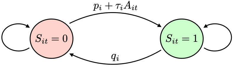
Figure 2: MDP for patient $i$.

This is a special case of the full model from Section 3.1, where we assume the patient MDP takes the simple form described above. All other aspects of the model remain the same. In particular, the system MDP is derived by combining the patient MDPs via a budget constraint and outreach interventions are costly and must therefore be rationed. Note that the set of possible policies is finite, since both the state and action spaces are finite. Therefore, for any instance, there exists an optimal policy $\mathsf{OPT}$ which maximizes the objective, $\mathbb{E}[\sum_{t=1}^{T}\sum_{i=1}^{N}S_{i,t+1}]$.

We believe this simplified version of the system is representative and relevant, both for our specific motivating application and behavioral health operations in general. From the perspective of Keheala (as described in Section 1), the stylized model captures the salient features of patient behavior in the simplest way possible. A dataset collected by an RCT run by Keheala revealed that the best single feature that predicted whether a patient will verify on a given day, is simply whether they verified the day before (80.9% accuracy). Therefore, the states in the model simply represent whether a patient verified the previous day. Next, the main objective of the outreach interventions for Keheala is to target patients who have not been verifying, to encourage them change their behavior. As a result, our model is such that the intervention only impacts the transition from state 0 to state 1.

More broadly, similar Markov models have been used in the literature to model patient behavior. Mate et al. (2020) and Mate et al. (2022) use the same two-state model and applied it to the setting of TB treatment adherence and maternal, health respectively. Biswas et al. (2021) also studies maternal health in which they employ a similar MDP with three states. Even the objective function $\mathbb{E}[\sum_{t=1}^{T}\sum_{i=1}^{N}S_{i,t+1}]$, which captures the platform’s goal of having its users be in the ‘desired’ state, has has been used in the literature (Mate et al. 2020, 2022, Biswas et al. 2021). This type of a two-state Markov model is originally from the literature on communication systems (where it is referred to as a Gilbert-Elliot channel (Gilbert 1960)) but has also been used in marketing (Schmittlein et al. 1987).

4.2 The $\mathsf{DecompPI}$ Policy for the Two-State MDP Model

Our main result pertains to $\mathsf{DecompPI}(\pi)$ for $\pi$ belonging to a class of policies. Specifically, for $\gamma\in(0,1)$, let $\mathsf{RAND}(\gamma)$ be the policy in which at every time step, gives an intervention to every patient in state 0 independently with probability $\gamma$. Denote the intervention values of the policy $\mathsf{RAND}(\gamma)$ by $z^{\gamma}_{it}\triangleq z^{\mathsf{RAND}(\gamma)}_{it}$ We will provide a performance guarantee for the policy $\mathsf{DecompPI}(\gamma)\triangleq\mathsf{DecompPI}(\mathsf{RAND}(\gamma))$.

Our focus is in the regime where $\gamma$ is small (close to 0), and we will see that the theoretical guarantees are stronger when this is the case. This represents a ‘budget-constrained’ regime; the probability of a patient receiving an intervention is small, or equivalently, the number of interventions given is small relative to the number of patients. To give intuition on the policy $\mathsf{DecompPI}(\gamma)$ in this regime, we provide a simple expression for the intervention value in the case where $\gamma\to 0$ and $T=\infty$.

Proposition 4.1

Suppose $T=\infty$. Then, $\lim_{\gamma\to 0}z^{\gamma}_{it}(0)=\tau_{i}/(p_{i}+q_{i})$ for any $i$ and $t$.

A more general version of Proposition 4.1 is proven as Lemma A2.7 in Appendix A2.1. Proposition 4.1 says that when $T=\infty$ and $\gamma\to 0$, $\mathsf{DecompPI}(\gamma)$ orders patients in state 0 by the index $\tau_{i}/(p_{i}+q_{i})$, and intervenes on those with the highest values. The index increases with $\tau_{i}$ and decreases with $p_{i}$ and $q_{i}$, which is intuitive. $\tau_{i}$ is the ‘treatment effect’ of an intervention on the probability that the patient switches from state 0 to 1. The smaller the value of $q_{i}$, the longer the patient will stay in state 1 once they are there, increasing the ‘bang-for-the-buck’ of an intervention. As for $p_{i}$, a larger value means that a patient is likely to move to state 1 without an intervention; hence lower priority is given to those with a large $p_{i}$.

4.3 Performance Guarantee

Let $\mathsf{NULL}$ be the policy that only takes the null action; i.e. $\mathsf{NULL}_{t}(\mathbf{S})=(0,\dots,0)$ for all $\mathbf{S},t$. As a slight abuse of notation, we use $\mathsf{OPT},\mathsf{NULL},\mathsf{RAND}(\gamma)$ and $\mathsf{DecompPI}(\gamma)$ to also denote the expected reward of those policies. We now state our main result, a performance guarantee for the policy $\mathsf{DecompPI}(\gamma)$.

Theorem 4.2 (Main Result)

Given an instance of the two-state model, let $\bar{M}=\max_{i\in[N]}\frac{\tau_{i}(1-p_{i}-q_{i})}{(p_{i}+q_{i})(1-p_{i})}>0$. For any $\gamma\in(0,1)$,

$$\mathsf{DecompPI}(\gamma)-\mathsf{NULL}\;\geq\;\frac{1}{2(1+\gamma\bar{M})}\;(\mathsf{OPT}-\mathsf{NULL}).$$ (3)

Theorem 4.2 provides an approximation guarantee for $\mathsf{DecompPI}(\gamma)$ with respect to the improvement over the null policy. The approximation ratio, $\frac{1}{2(1+\gamma\bar{M})}$ depends on two quantities: $\gamma$ is a parameter of the policy $\mathsf{RAND}(\gamma)$ which is used to compute the intervention values, and $\bar{M}$ is a quantity related to the instance parameters, $\{(p_{i},q_{i},\tau_{i})\}_{i\in[N]}$. For any fixed instance, the approximation ratio improves as $\gamma$ decreases, approaching 1/2 as $\gamma$ goes to 0. Therefore, as $\gamma\to 0$, $\mathsf{DecompPI}(\gamma)$ achieves at least half of the improvement in reward as compared to that of the optimal policy.

With respect to $\bar{M}$, a smaller value implies a stronger guarantee. Since we assume $p_{i},q_{i}\leq 1/2$, $\bar{M}\leq\max_{i\in[N]}\frac{\tau_{i}}{p_{i}+q_{i}}$. For $\bar{M}$ to be small, it must be that $p_{i}+q_{i}$ is bounded away from 0 for all $i$ — specifically, patients must not be completely sticky, where sticky means that they never switch their state, no matter which state they are in.

Theorem 4.2 is significantly stronger than and implies the usual notion of an approximation result, which is the following:

Corollary 4.3 (Weaker result)

For any problem instance of the two-state model, $\mathsf{OPT}\leq\frac{1}{2(1+\gamma\bar{M})}\mathsf{DecompPI}^{*}$.

Because a patient can transition from state 0 to 1 without an intervention (if $p_{i}>0$), the $\mathsf{NULL}$ policy can achieve a significant fraction of $\mathsf{OPT}$. If it was the case that $\mathsf{NULL}$ is more than half of $\mathsf{OPT}$, then Corollary 4.3 would be vacuous. On the other extreme, if an intervention was necessary for all patients to transition to state 1 (i.e. $p_{i}=0$ for all $i$), then it would be that $\mathsf{NULL}=0$, in which case the result of Theorem 4.2 is equivalent to that of Corollary 4.3.

4.4 Robustness under an Approximate Implementation

Note that Theorem 4.2 assumes that the intervention values are known exactly. In practice, these intervention values must be estimated, as discussed in the intended usage in Section 3.3. We show that this result is robust, in the sense that a policy that approximately implements $\mathsf{DecompPI}(\lambda)$ also yields a performance guarantee.

Suppose $\mathsf{ALG}$ is an index policy using indices $z^{\mathsf{ALG}}_{it}(0)$. That is, $\mathsf{ALG}$ assigns interventions to the patients in state 0 with the largest value of $z^{\mathsf{ALG}}_{it}(0)$. Then, we show that if the index values $z^{\mathsf{ALG}}_{it}(0)$ approximate the intervention values $z^{\lambda}_{it}(0)$, then $\mathsf{ALG}$ also admits a performance guarantee.

Theorem 4.4

Suppose $\mathsf{ALG}$ is an index policy that uses index values $z^{\mathsf{ALG}}_{it}(0)$ that satisfies, for all $i$ and $t$,

$$\beta_{1}z_{it}^{\lambda}(0)\leq z^{\mathsf{ALG}}_{it}(0)\leq\beta_{2}z_{it}^{\lambda}(0),$$ (4)

for some $\beta_{1}\leq 1$ and $\beta_{2}\geq 1$. Then,

$$\mathsf{ALG}-\mathsf{NULL}\;\geq\;\frac{\beta_{1}}{\beta_{2}}\cdot\frac{1}{2(1+\gamma\bar{M})}\;(\mathsf{OPT}-\mathsf{NULL}).$$

The proof can be found in Appendix A2.6. This result implies that one does not have to run $\mathsf{DecompPI}$ exactly in order to achieve good performance. In practice, one may estimate the intervention values from data — even if the estimation is not perfect, Theorem 4.4 ensures a performance guarantee.

5 Case Study: TB Treatment Adherence

In this section, we revisit the full problem (introduced in Section 3) and conduct numerical experiments to evaluate the performance of $\mathsf{DecompPI}$ for its intended use case. Our analysis is motivated by our partner organization, Keheala, which operates a digital health platform to support medication adherence among TB patients in highly resource-constraint settings. Here, we first summarize the state of the global TB epidemic and the Keheala behavioral intervention (Section 5.1). We then describe our data sources and the validated simulation model we have developed to test outreach policies (Section 5.2 and Section 5.3). Next, we discuss how our policy, as well as some benchmark policies, can be implemented using Keheala’s data (Section 5.4), before presenting our numerical results (Section 5.5).

5.1 The global TB epidemic and the Keheala intervention

TB remains one of the deadliest communicable diseases in the world, causing 1.6 million deaths in 2021. This is remarkable in light of the fact that effective treatment has been available for over 80 years, with the current WHO guidelines recommending a 6 month regimen of antibiotics for drug-susceptible TB and a more intense regiment for drug-resistant strains (WHO 2022). A key limiting factor for curbing the epidemic is lack of patient adherence to these treatment regiments, which increases the probability of infection spreading, drug resistance, and poor health outcomes (Garfein and Doshi 2019).

Keheala was designed to provide treatment adherence support to TB patients in resource-limited settings. Their platform operates on the Unstructured Supplementary Service Data (USSD) mobile phone protocol, which importantly allows phones without smart capabilities to access the service. Once a patient has enrolled with Keheala, they are meant to self-verify treatment adherence every day, using their mobile phone. In addition, they have access to a range of services. Some are on-demand, for example educational material about TB or leaderboards for verification rates. Others are automatic, such as adherence reminders, which are sent to patients daily (at their pre-determined medication time) in the absence of verification. In addition, the Keheala protocol is to escalate outreach interventions when patients do not self-verify adherence. It states that after one day of non-adherence patients should receive a customized message to encourage resumed adherence and after two days of non-adherence patients should receive a phone call from a support sponsor. While these support sponsors are full-time employees, they are not healthcare professionals. They are members of the local community who have experience with TB treatment and are therefore familiar with the many contributing factors associated with low treatment adherence, such as side-effects, societal stigma against TB patients, and challenges with refilling prescriptions.

The overall effectiveness of Keheala’s combination of services was evaluated in a randomized controlled trial (RCT) in Nairobi, Kenya. The trial demonstrated that Keheala reduced unsuccessful TB treatment outcomes—a composite of loss to follow-up, treatment failure, and death—by roughly two-thirds, as compared to a control group that received the standard of care (Yoeli et al. 2019). Given this success, Keheala’s primary practical objective is to ensure that enrolled patients remain engaged with the platform through adherence verification.

In this paper, we focus on the final level in Keheala’s escalation protocol—support sponsors making phone calls to patients. This part of the outreach was organized through populating a daily list of patients who had not verified treatment adherence for 48 hours. Support sponsors had many responsibilities in operating the platform, but would make phone calls to as many patients on the list as possible on a given day. Since hiring support sponsors is a costly aspect of operating the service, Keheala is interested in implementing a more personalized and targeted approach for prioritizing which patients should receive a phone call on a given day. Being able to maintain a similar performance with fewer support sponsors (or equivalently, serve more patients with the same number of support sponsors) is desirable for any future scale-up of the system.

5.2 Data sources.

Based on the success of the first RCT, the effectiveness of Keheala was further evaluated in a second RCT during 2018-2020. The RCT was conducted in partnership with 902 health clinics distributed across each of Kenya’s eight regions, representing a mix of rural and urban clinics. The study included four treatment arms and enrolled over 15,000 patients. We obtained data for 5,433 patients enrolled in the Keheala intervention arm (other arms aimed to independently test specific components of the Keheala intervention).

As part of the RCT, the study team collected socio-demographic information from all patients. This information includes static covariates such as age, gender, language preferences, location, as well as limited clinical history (see Section A4.1 for a full list). In addition, Keheala collected engagement data about each patient during their enrollment in the service. This includes whether a patient verified on a given day, how many reminders they received, and whether they were contacted by a support sponsor.

After filtering out patients with missing information or not enough data, we conducted all our analysis on 3594 patients. The average patient was enrolled on the platform for 118 days. On an average day, 608 patients were enrolled and 210 of those were eligible for a support sponsor call according to the protocol (i.e., having not verified treatment adherence for the preceding 48 hours). The support sponsors, employed by Keheala, had a range of responsibilities in operating the platform, including making outreach phone call so to the eligible patients. The average number of support sponsors making calls to patients on a given day was 3 and the average number of calls made was 25.5. Hence, in our analysis, we use a budget of $B$ = 26 as our main point of comparison.

5.3 Simulation Model.

We build a simulation model that we use to estimate the counterfactual outcomes of different outreach approaches. The simulator is effectively represented by a single function, $f(s,a)\in[0,1]$, which denotes the probability that a patient in state $s$ with action $a$ verifies in the next time step. This function is used to simulate one step transitions for every patient. We first describe the state space of the patients, describe the exact simulation procedure, and then discuss how we learn $f$ from data and validate the simulator.

5.3.1 Patient state space.

For patient $i$, let $X_{i}\in\mathbb{R}^{13}$ be their static covariates. Let $V_{it}\in\{0,1\}$ denote whether patient $i$ verified at time $t$, and let $A_{it}\in\{0,1\}$ denote whether the patient received the intervention at time $t$. Let $H_{it}=(V_{i1},A_{i1},\dots,V_{i,t-1},A_{i,t-1},V_{it})\in\mathbb{R}^{2t-1}$ be the history of verifications and interventions up to time $t$. We define a condensed history $\tilde{H}_{it}\in\mathbb{R}^{21}$ by summarizing the history $H_{it}$ into 21 features, aiming to capture as much relevant information as possible. The condensed history contains the patient’s recent and overall behavior. For statistics such as the number of times the patient verified and the number of interventions they have received, we aggregate them over the past week, as well as in total. We also include information on their verification and non-verification streaks, as well as how long they have been in the platform. See Section A4.1 for a full list of these features. Then, we define the state of patient $i$ at time $t$ to be $S_{it}=(X_{i},\tilde{H}_{it})\in\mathbb{R}^{34}$.

5.3.2 Simulation procedure.

Given $f$ and an intervention policy $\pi$, we ‘mimic’ the RCT by simulating patient behavior day by day. In total, we simulate $T=700$ time steps, where each $t\in[T]$ corresponds to one day between April 2018 to March 2020. We let $T_{s}(i)$ and $T_{e}(i)$ denote the starting and ending time steps that patient $i$ was enrolled in Keheala. Each patient $i$ is then introduced into the system at time $t=T_{s}(i)$, and removed at time $t=T_{e}(i)$. We use the observed data from the RCT for their first 7 days in the system to initialize their state. Then, in each time period $t$, we let $P_{t}$ be the set of patients that were active in the RCT for more than 7 days. We use some policy $\pi$ for the patients $P_{t}$ to determine who receives sponsor outreach. If a patient $i$ was in state $S_{it}$ at time $t$ and the policy $\pi$ chose action $A_{it}$, we let $V_{i,t+1}$ be 1 with probability $f(S_{it},A_{it})$, and 0 otherwise (and randomness is independent across patients and time steps). Finally, we use $V_{i,t+1}$ to update their state for the next time step.

5.3.3 Estimating the $f$ function.

Using the state space $\mathcal{S}$ as described above, we construct the function $f:\mathcal{S}\times\{0,1\}\to[0,1]$ using data from the RCT. Specifically, we learn the two functions $f(s,0)$ and $f(s,1)$ separately. For $f(s,0)$, we train a gradient boosting classifier on the dataset $\{(S_{it},V_{i,t+1})\}_{i\in N,t\in[T]:A_{it}=0}$, using $V_{it}$ as the outcome variable. For $f(s,1)$, we write the function as $f(s,1)=f(s,0)+\tau(s)$ and we learn $\tau(s)$ using the double machine learning method of estimating heterogeneous treatment effects (Chernozhukov et al. 2018). See Section A4.2 for details on implementing this method.

5.3.4 Train and test split.

Importantly, we use a different set of patients to estimate the $f$ function (and to run our simulations) from the set of patients we use to train our policies. In particular, we randomly split all patients from the RCT into two groups, which we call train and test. We use the test set to estimate the $f$ function that forms the basis for the simulation model. We keep the train set of patients separate and use it to train policies (see Section 5.4, below). This ensures that the policies we evaluate are not learned off of the same dataset that was used for the simulations. The simulation itself uses the test patients, and we duplicated each patient so that we maintain a similar total number of patients as in the original study.

5.3.5 Simulation validation.

We validate the performance of the simulator on a different intervention policy than the simulator was trained on, by leveraging the fact that there was variability in the number of interventions given throughout the RCT. In particular, the average number of interventions given during the first half of the RCT was around double of that of the latter half (45.9 vs. 21.4), and this variation induces a change in the intervention assignment policy. Then, dividing the data into halves produces two datasets that are generated using effectively different intervention policies — that is, the distribution of the observed states of patients are different between the two datasets.

To validate the simulator, we use the method from Section 5.3.3 to learn $f$ using the first dataset, and then validate its performance on the second dataset. Using this procedure, the AUCs on the second dataset for $f(s,0)$ and $f(s,1)$ were 0.918 and 0.745, respectively. We also check the calibration of both of these functions, by grouping the samples into bins based on their predicted probability of verifying the next day, and checking whether their actual verification rates.

We group the samples based on the simulated probability of verification into bins with a 10% range, and we compute the expected calibration error (ECE) (Naeini et al. 2015). For bin $i$, let $o_{i}$ be the true fraction of positive instances in bin $i$, $e_{i}$ be the mean of the predicted probabilities of the instances in bin $i$, and $N_{i}$ be the number of samples in bin $i$. Then, the ECE is defined as

$$\text{ECE}=\frac{1}{N}\sum_{i=1}^{10}N_{i}|o_{i}-e_{i}|,$$ (5)

where $N$ is the total number of samples. The expected calibration error was 0.0066 for $f(s,0)$ and 0.0308 for $f(s,1)$. Figure 3 displays these bins.

These results demonstrate that the simulator has good performance in mimicking patient behavior. As expected, the AUC and the ECE is worse for $f(s,1)$ compared to $f(s,0)$; this is due to the significantly fewer number samples with an intervention in the training data, as well as the increase in variance of doing off-policy estimation. The training data used for $f(s,0)$ had 300K samples, while the one used for $f(s,1)$ had 4.5K samples. For $f(s,1)$, the calibration is slightly off for samples with a high probability of verification (bins 0.7-0.9); however, we note that the 0.7-0.9 bins only contain 11.3% of all samples for $f(s,1)$.

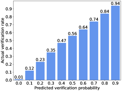
(a) Calibration for $f(s,0)$

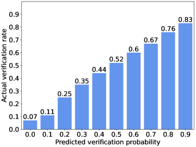
(b) Calibration for $f(s,1)$

Figure 3: Calibration plots for $f(s,0)$ and $f(s,1)$ for simulation validation. We group the samples based on the simulated probability of verification into bins with a 10% range, which we label by the lower number. For example, the 0.3 bin on the x-axis represents the samples whose probability of verification according to $f$ is in $[0.3,0.4)$; hence we should expect the actual number of verifications of those samples to be around 0.35.

5.4 Outreach Policies and Experimental Design

Using the simulation model described above, we compare the performance of three main policies. For each policy, we vary the budget for outreach interventions per day between 10 and 40. As mentioned before, the average number of sponsor outreaches during a given day of the trial was 26. Importantly, we restrict all policies so that they can only provide an outreach to patients who have not verified for at least two days in a row. This is because that was what was done in the RCT, hence there is no data for how an outreach affects behaviors for those who do not meet this criterion. Therefore, we would not be able to accurately evaluate policies that do not follow this restriction.

We note that attaining improved performance with lower outreach capacity is particularly important for the resource-limited setting at hand as it speaks to the performance achievable during a future scale-up of the system, in which the ratio of patients to support sponsors is likely to be much higher.

Below, we describe the four policies implemented, starting with a description of how to implement our $\mathsf{DecompPI}$ policy, before describing the benchmark approaches.

5.4.1 $\mathsf{DecompPI}$ for Keheala.

The first step in operationalizing $\mathsf{DecompPI}$ is defining the state space for each patient. For this, we use the same condensed state space as described in Section 5.3.1, i.e., we define the state of patient $i$ at time $t$ to be $S_{it}=(X_{i},\tilde{H}_{it})\in\mathbb{R}^{34}$ (a full list of these features is included in A4.1). Importantly, we note that all of the features of this state space are observable to Keheala at any time $t$, once a patient has been enrolled on the platform for seven days.

The second step is estimating the $\hat{z}_{it}(S_{it})$ score for each patient at each time period, which is ultimately used to prioritize patients. As before, we let $T_{s}(i)$ and $T_{e}(i)$ be the starting and ending time steps that patient $i$ was enrolled in Keheala. Using this notation, we can represent the future verification rate for patient $i$ at time $t$ by $y_{it}=\frac{1}{T_{\text{e}}(i)-t}\sum_{r=t+1}^{T}V_{ir}$. Then, the data from the RCT can be written in the form $\{(S_{it},a_{it},y_{it})\}_{i\in[N],t\in\{T_{s}(i),\dots,T_{e}(i)\}}$, and we can estimate the function $q_{it}^{\mathsf{Baseline}}(s,a)$ using this data. In our implementation, we use a linear function approximation for the verification rate, assuming the form

$$q_{it}^{\mathsf{Baseline}}(s,a)=\langle\theta_{a},s\rangle\cdot(T_{\text{e}}(i)-t),$$

for each of the two actions $a\in\{0,1\}$. The $\langle\theta_{a},s\rangle$ term represents the future verification rate, and $T_{\text{e}}(i)-t$ represents the number of days left. We note that the state contains information regarding the number of days the patient has been enrolled in Keheala, hence the verification rate is also a function of the time step.

We estimate $\theta_{a}$ using least squares with an $\ell_{2}$ regularizer:

$$\hat{\theta}_{a} \in\argmin_{\theta\in\mathbb{R}^{34}}\bigg{(}\sum_{i\in N}\sum_{t=T_{\text{s}}(i)}^{T_{\text{e}}(i)}\mathbbm{1}(a_{it}=a)(y_{it}-\theta^{\top}S_{it})^{2}+||\theta||^{2}_{2}\bigg{)}.$$ (6)

Finally, we compute a patient’s estimate of their intervention value at time $t$ as

$$\hat{z}_{it}(S_{it})=\langle\hat{\theta}_{1}-\hat{\theta}_{0},S_{it}\rangle\cdot(T_{\text{e}}(i)-t),$$

and the resulting policy is to give the intervention to up to $B$ patients with the highest positive $\hat{z}_{it}(S_{it})$ values.

5.4.2 Bandit.

The bandit policy aims to choose patients with the highest increase in the probability of next-day verification, using a linear contextual bandit model. In terms of the 2-state model from Section 4.1, the goal is to choose patients with the highest value of $\tau$. We essentially use the same state space and linear model as was used for $\mathsf{DecompPI}$, except that the outcome variable is next-day verification, rather than total future verifications. We first learn a prior using the offline data, and then we run a Thompson sampling style policy, which continually updates the policy with online data.

Specifically, we assume the linear form $V_{i,t+1}=\langle\beta_{a},S_{it}\rangle$ for action $a\in\{0,1\}$, with unknown parameters $\beta_{0},\beta_{1}\in\mathbb{R}^{34}$. The prior on $(\beta_{0},\beta_{1})$ is initialized as the output of a least-squares regression using the offline data, the same data that was used to train $\mathsf{DecompPI}$. At each time step, $(\tilde{\beta_{0}},\tilde{\beta_{1}})$ is sampled from the posterior. Then, the policy chooses the $B$ patients with the highest value of $\langle\tilde{\beta_{1}},S_{it}\rangle-\langle\tilde{\beta_{0}},S_{it}\rangle$. After the outcome is observed at each time step, the posterior is updated accordingly. The detailed description on the algorithm can be found in Section A4.3.

We note that this policy makes use of strictly more data than $\mathsf{DecompPI}$, since $\mathsf{DecompPI}$ only uses the offline data. In the results, we confirm that this policy indeed learns myopic rewards correctly. Therefore, this is a very strong benchmark algorithm for optimizing myopic rewards.

5.4.3 Whittle’s index (QWI).

The next benchmark is the Whittle’s index. The advantage of this method compared to the bandit benchmark is that is is non-myopic. However, the downside is that computing the Whittle’s index requires the model to be known. To implement Whittle’s index in our setting where the model is unknown, we leverage the recent work of Avrachenkov and Borkar (2022) who propose a Q-learning approach to learn the Whittle’s index, which we refer to as $\mathsf{QWI}$. $\mathsf{QWI}$ is an online learning method that simultaneously learns the Q-values as well as the Whittle’s index for each state.

There are two main challenges in implementing $\mathsf{QWI}$ in our setting. The first is that the algorithm is an online learning method, and the second is that it requires a finite state space as it learns the Whittle’s index for each state separately. For the first point, we adapt the algorithm from Avrachenkov and Borkar (2022) to an offline setting so that it can use the same data that is used to train $\mathsf{DecompPI}$. Although we could simply run $\mathsf{QWI}$ as a fully online algorithm (without leveraging the offline data), we believe that this would lend an unfair comparison against $\mathsf{DecompPI}$. For the second point, we define a smaller, finite state space so that $\mathsf{QWI}$ can be implemented. Specifically, we incorporate the most relevant information, which we found to be information regarding the patients’ history of verifications as well as the number of past interventions. We use this information to define a state space with 45 states in total. Details on this state space, as well as details of the offline learning method is deferred to Appendix A4.4.

Based on this state space, we learn the Whittle’s index, $\lambda(u)\in\mathbb{R}$, for each state $u$. Then, at each point in time, $\mathsf{QWI}$ chooses the patients in states with the highest Whittle’s index to give the intervention to.

5.4.4 Baseline.

Our baseline policy approximates the heuristic followed by Keheala in the two RCTs that have been implemented. In both cases, the protocol was that patients were added to the support sponsor call queue after not verifying for 48 hours. As a result, the order of patients in the queue is effectively random, determined by a combination of their designated medication time (which prompts automated reminders to take the medicine and verify) and the timing of their self-verification. We approximate the resulting outreach policy by selecting $B$ patients out of all those who have not verified for 48 hours, at random.

5.5 Results

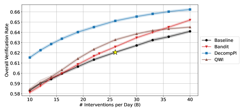
Figure 4: Average overall verification rate over 50 runs for each policy and budget. The shaded region indicates a 95% confidence interval. The star represents the operating point for Keheala.

5.5.1 Overall performance.

The average performance for each budget and policy over 50 runs are shown in Figure 4, which shows that $\mathsf{DecompPI}$ clearly outperforms the other policies over a wide range of budget values. For a practical interpretation of the results, consider Baseline at a budget of 26, the policy and budget that Keheala was operating during the RCT, which results in an overall verification rate of 62.0%. By using less than half of the budget, $B=12$, $\mathsf{DecompPI}$ achieves the same verification rate at 62.2%. As the costliest aspect of Keheala’s system is in hiring staff to provide the interventions, these results imply that they can cut these costs by half to achieve the same outcome.

Additionally, we observe that the improvement of $\mathsf{DecompPI}$ compared to the other policies is especially substantial for smaller budgets. This implies that when the number of patients that can be targeted is small, $\mathsf{DecompPI}$ can correctly identify the set of patients to target that result in the largest gains. This is especially valuable for scaling up the system. Indeed, if Keheala wanted to expand to include more patients without linearly increasing their staff costs, then the ratio of budget to the number of patients would decrease, resulting in the regime where $\mathsf{DecompPI}$ offers major improvements.

The fact that the performance of $\mathsf{Bandit}$ policy improves over $\mathsf{Baseline}$ as the budget increases is caused by the increase in relevant data. Note that the number of interventions is small ($\sim 26$) relative to the total number of patients in the system ($\sim 600$), implying that the number of data points with $A=1$ is much smaller than that of $A=0$. Therefore, the main bottleneck in estimation is learning patient behaviors after receiving an intervention. As the budget increases, the $\mathsf{Bandit}$ has access to more data from patients with an intervention, and hence is able to improve its learning.

$\mathsf{QWI}$ has a slightly inconsistent performance curve relative to the other policies. Its performance is always better than or similar to $\mathsf{Baseline}$, but compared to $\mathsf{Bandit}$, it over-performs in the mid-budget regime, but under-performs as the budget increases. We dive deeper into the types of patients each policy targets in Section 5.5.3, where we provide an explanation for this behavior.

5.5.2 Patient-level verification rates.

The overall number of verifications increases under $\mathsf{DecompPI}$, but how do these rates get impacted at the patient-level? Fixing the budget to be 26, we compute the verification rate of each patient, and we examine the distribution of these patient-level rates. In Figure 5, we plot the difference in the number of patients that had a particular verification rate under $\mathsf{DecompPI}$ versus $\mathsf{Baseline}$. We see that under $\mathsf{DecompPI}$, fewer patients have a low verification rate (less than 40%), and the number of patients with a moderately high verification rate (60%-90%) increases. Overall, this represent a desirable type of shift, where main improvement of $\mathsf{DecompPI}$ comes from an increase in the number of patients with a high verification rate.

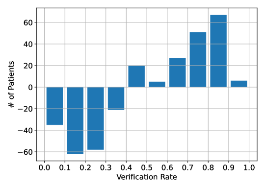
Figure 5: Difference in patient verification rates under $\mathsf{DecompPI}$ compared to $\mathsf{Baseline}$. The bins represent the difference in the number of patients whose overall verification rate is between $0-10\%$, $10-20\%,\dots,90-100\%$. There were 3594 patients in total.

Now, another obvious metric of interest is eventual health outcomes. Unfortunately, it is difficult to determine how a new policy will affect health outcomes since it is not known exactly how increased self-verification of treatment adherence translates into improved health outcomes. What is known is that (a) patients who are enrolled on the Keheala platform have much lower rates of undesired outcomes (e.g., treatment failure) than patients who only receive the standard of care (undesired outcomes drop by about two-thirds, according to Yoeli et al. (2019)) and (b) higher self-verification rates are associated with better outcomes, among patients who are enrolled on the platform (Boutilier et al. 2022). However, making precise statements about how self-verification affects outcomes remains a very interesting open problem.

5.5.3 Description of the targeted patients.

In Table 1, we fix the budget to be 26 and we show statistics regarding the state of the targeted patients for each of the four policies. For example, under $\mathsf{Baseline}$, on average, the patient that received an intervention had a treatment effect of 8.8% with respect to the probability that they will verify the next day. 8.8% is the ‘true’ average treatment effect, in the sense that the numbers that are averaged are taken directly from the simulation model.

Table 1: Average statistics of the state of patients who were given an intervention, across the three policies that were run for $B=26$. (a) is the average value of $\tau(x)$, the increase in probability that the patient verifies the next day when they are given an intervention. (b) is the average $f(x,0)$, the probability that a patient verifies the next day without an intervention. (c) is the average number of remaining days the patient will be on treatment for.

	$\mathsf{Baseline}$	$\mathsf{Bandit}$	$\mathsf{DecompPI}$	$\mathsf{QWI}$
(a) Next-day treatment effect	8.8%	13.2%	10.6%	6.9%
(b) Next-day base probability	18.2%	35.2%	22.2%	12.2%
(c) Days on treatment remaining	68.3	92.4	109.3	69.7

Statistic (a) represents exactly what the $\mathsf{Bandit}$ policy optimizes for, the increase in probability of the patient verifying the next day. The fact that $\mathsf{Bandit}$ yields the highest value confirms that indeed, the policy correctly learns what it is supposed to learn. $\mathsf{DecompPI}$ chooses patients with a higher one-step treatment effect than $\mathsf{Baseline}$, but lower than that of $\mathsf{Bandit}$. Then, the fact $\mathsf{DecompPI}$ outperforms $\mathsf{Bandit}$ in terms of overall verification implies that a myopic strategy of looking only one step ahead is not sufficient. The next two statistics shed light on why this may be.

Statistic (b) represents the probability that the targeted patient would have verified anyway without an intervention, and we see that the $\mathsf{Bandit}$ targets patients with a much higher base probability than the other policies. We plot the entire distribution of this quantity in Figure 6, where we see that $\mathsf{Bandit}$ often targets those with a relatively high base probability ($>45\%$), while $\mathsf{DecompPI}$ targets those with a relatively low base probability ($<15\%$). This may contribute to the improved performance of $\mathsf{DecompPI}$, and reasoning for this can be seen through the 2-state model from Section 4.1, where the base probability corresponds to the parameter $p$. If two patients have the same values of the parameters $q$ and $\tau$ but differing values for $p$, the intervention value is higher when $p$ is smaller (see Proposition 4.1). This is because the patient with a high value of $p$ is more likely to switch to state 1 at the current time step as well as all future time steps. As an extreme example, for a patient with $p=0$, they need an intervention to switch to state 1, whereas a patient with $p>0$ may switch to state 1 (either now or in the future), without an intervention. Therefore, an intervention is more likely to be helpful for those with a smaller base probability, which $\mathsf{DecompPI}$ targets.

On the other hand, $\mathsf{QWI}$ takes the above strategy to an extreme, where it targets those with a very low base probability (12.2%), but on average these patients also do not have a high next-day treatment effect (6.9%). This may explain the inconsistent behavior of $\mathsf{QWI}$ as the budget increases. The strategy of targeting these patients with a low base probability and a low treatment effect is reasonably effective in the mid-budget regime; however, as the budget increases, one may also need to judiciously target other types of patients, which $\mathsf{QWI}$ does not do. Now, one approach that may potentially improve the performance of $\mathsf{QWI}$ is to change the way that the state space is defined. For a policy to target patients in a more fine-grain, personalized manner requires a corresponding finer-grained state space. However, a larger state space would suffer from a larger estimation error given the same size of the dataset. This is one of the main downsides of QWI — the algorithm designer is faced with a non-trivial challenge of defining an appropriate finite-sized state space for the problem at hand.

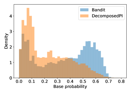
Figure 6: Histogram of the base probability of targeted patients, the probability that the patients would verify without an intervention. This is the entire distribution of the statistic (b) in Table 1 for $\mathsf{Bandit}$ and $\mathsf{DecompPI}$.

Lastly, statistic (c) is the average number of days a targeted patient has remaining on the platform. If an intervention positively affects patients for all of their future time steps, then targeting those with longer time left in the system would result in higher benefits. The results show that $\mathsf{DecompPI}$ targets those with the longest days of treatment left.

5.5.4 Prominent features for $\mathsf{DecompPI}$.

Table A1 displays the five most predictive features of the intervention values that $\mathsf{DecompPI}$ uses to target patients. These features were found by using Lasso regression with a tuned parameter – see Section A4.5 for details on the method used. The results show that the intervention value is lower when the number of previous interventions is higher (first two features), which is intuitive since patients may become fatigued and less receptive when there are too many interventions. The intervention value is lower when the patient’s past verifications is higher (third and fourth features). This is consistent with the analysis in Table 1, where $\mathsf{DecompPI}$ targets those with a smaller next-day base probability of verifying. Lastly, the intervention value increases for patients who are older.

Table 2: The most predictive features of higher intervention values for $\mathsf{DecompPI}$, as well as the sign of their coefficient.

Feature	Sign of Coefficient
Interventions: total number	$-$
Interventions: # previous week	$-$
Verifications: overall percentage	$-$
Verifications: # previous week	$-$
Age	$+$

6 Conclusion and Future Directions

This work tackles an important problem of personalizing and optimizing costly interventions in the context of digital systems for behavioral health. We develop an approach, $\mathsf{DecompPI}$, that learns an intervention policy from an existing dataset collected from a pilot study. $\mathsf{DecompPI}$ is model-free, which avoids the need to specify a model of patient behaviors. Unlike many reinforcement learning methods which often rely on a long horizon to achieve good performance, $\mathsf{DecompPI}$ leverages offline data to immediately provide an effective policy. We provide a theoretical guarantee on a special case of the model that represents the practical setting of interest, and it exhibits strong empirical performance on a validated simulation model of a real-world behavioral health setting.

Limitations and future directions. Lastly, we discuss limitations of the current work that serve as valuable future directions. One gap between our model and the practical application of Keheala is that the ultimate objective of Keheala is to improve eventual health outcomes (i.e., cure patients of TB). There are two major hurdles that need to be addressed in order to fully align with this goal, within the existing infrastructure of Keheala (of using daily adherence information). The first obstacle is the lack of a mapping between treatment adherence patterns to health outcomes. It has been shown that higher verification rates are associated with better outcomes (Boutilier et al. 2022) but it would be valuable to identify more specific and causal relationships (e.g., is it more important for a patient to adhere to their treatment in the earlier phase of their treatment regime compared to later?). Addressing this issue is very specific to TB but would be tremendously valuable not only for optimizing a platform like Keheala, but also for the broader medical research on TB. Second, a problem less specific to TB, is to design policies that can optimize for reward functions which are not necessarily additive for each time step (e.g., maximize the number of patients whose overall verification percentage is over 70%).

Next, there are other interesting extensions to the model and the algorithm that one can consider. With respect to performance guarantees on the stylized model in Section 4, it would be valuable to analyze how the guarantee is impacted by various modeling extensions such as generalizing the MDP (e.g., more states, having interventions impact all states), or extending the class of base policies. From an algorithmic standpoint, valuable extensions include incorporating online samples, and incorporating other practical considerations such as fairness in how the interventions are distributed across patients.

E-companion for “Targeted interventions for TB treatment adherence”

A1 Table of Notation

Table A1: List of notation used in the paper and the proofs in Section A2.

Notation	Meaning
$N$	Number of patients
$T$	Number of time steps
$B$	Budget
$\mathcal{S}$	State space for a single patient
$\mathcal{A}$	Action space for a single patient
$\mathcal{A}^{N}$	Action space for the system
$P_{i}(s,s^{\prime},a)$	Transition probability function for patient $i$
$R_{i}(s,s^{\prime},a)$	Reward function for patient $i$
$S_{it}^{\pi}$	State of patient $i$ at time $t$ under policy $\pi$
$A_{it}^{\pi}$	Action for patient $i$ at time $t$ under policy $\pi$
$q_{it}^{\pi}(s,a)$	Patient-level $q$-value defined in (1)
$z_{it}^{\pi}(s)$	Intervention value used for $\mathsf{DecompPI}(\pi)$
$p_{i},q_{i},\tau_{i}$	Parameters for the 2-state model of Section 4.1
$\gamma$	Probability of an intervention for the policy $\mathsf{RAND}(\gamma)$
$\bar{M}$	Instance-dependent parameter used in Theorem 4.2
$V_{it}$	Whether patient $i$ verifies at time $t$
$P_{it},Q_{it},K_{it},W_{it}$	Bernoulli variables used in the sample path coupling of Section A2.1
$\bar{z}_{it}(s)$	Null intervention values defined as $\lim_{\gamma\to 0}z_{it}^{\gamma}(s)$
$\mathsf{DecompPI}_{0}$	Index policy that ranks patients by the null intervention values
$I_{t}$	Subset of patients in state 0 at time $t$
$D_{t}(I)$	Subset of patients that $\mathsf{DecompPI}_{0}$ would choose out of $I\subseteq[N]$
$\mathsf{ONE}(i,t)$	Policy that chooses patient $i$ once at time $t$
$\tilde{S}_{ir|t}$	State of patient $i$ at time $r$ under $\mathsf{ONE}(i,t)$
$Z_{it}$	Number of times state of patient $i$ differ in $\mathsf{ONE}(i,t)$ compared to $\mathsf{NULL}$, defined in (A8)
$\tau_{i}(t)$	Last time before $t$ that $i$ was in state 0, defined in (A15)

A2 Proof of Theorem 4.2 and Theorem 4.4

We first prove Theorem 4.2, where we break down the proof into four steps, where the bulk of the proof lies in the first two steps. The proof of Theorem 4.4 follows from steps 3 and 4, which we describe in Section A2.6. The proofs of all of the steps make use a specific sample path coupling procedure which we describe in the next subsection.

Step 1.

First, we define null intervention values as $\bar{z}_{it}(s)=\lim_{\gamma\to 0}z^{\gamma}_{it}(s)$. We show that for any algorithm $\mathsf{ALG}$, the difference $\mathsf{ALG}-\mathsf{NULL}$ can be written as a sum of the null intervention values of the patients that were chosen.

Proposition A2.1

For any algorithm $\mathsf{ALG}$,

$$\mathsf{ALG}-\mathsf{NULL}=\mathbb{E}\left[\sum_{t=1}^{T}\sum_{i\in A^{\mathsf{ALG}}_{t}}\bar{z}_{it}(0)\right].$$ (A1)

Step 2.

Then, we define the policy $\mathsf{DecompPI}_{0}$ to be the policy which orders patients in state 0 with respect to the null intervention values, $\bar{z}_{it}(0)$, gives interventions to the $B$ patients with the highest values. We show that this policy achieves at least half of the optimal improvement over $\mathsf{NULL}$.

Proposition A2.2

For any instance of the 2-state model,

$$\mathsf{DecompPI}_{0}-\mathsf{NULL}\;\geq\;\frac{1}{2}\;(\mathsf{OPT}-\mathsf{NULL}).$$ (A2)

Step 3.

Next, we show that if a policy uses an index rule with indices that approximate the null intervention values, this policy also yields a performance guarantee.

Proposition A2.3

Fix $\alpha_{1}\in(0,1]$ and $\alpha_{2}\geq 1$. Let $\mathsf{ALG}$ be an index policy that uses indices $z^{\mathsf{ALG}}_{it}(0)$ that satisfy $\alpha_{1}\bar{z}_{it}(0)\leq z^{\mathsf{ALG}}_{it}(0)\leq\alpha_{2}\bar{z}_{it}(0)$ for all $i$ and $t$. Then,

$$\mathsf{ALG}-\mathsf{NULL}\;\geq\;\frac{\alpha_{1}}{2\alpha_{2}}\;(\mathsf{OPT}-\mathsf{NULL}).$$ (A3)

Step 4.

Lastly, we show that the intervention values $z^{\gamma}_{it}(0)$ satisfy the above, where the corresponding $\alpha$ is a function of both $\gamma$ and the underlying parameters.

Proposition A2.4

Fix a patient $i$, and let $M_{i}=\frac{\tau_{i}(1-p_{i}-q_{i})}{(p_{i}+q_{i})(1-p_{i})}>0$. For any $t\in[T]$, the intervention values $z^{\gamma}_{it}(0)$ and $\bar{z}_{it}(0)$ satisfy the following relationship:

$$\frac{1}{1+\gamma M_{i}}\bar{z}_{it}(0)\;\leq\;z^{\gamma}_{it}(0)\;\leq\;\bar{z}_{it}(0).$$ (A4)

Using Proposition A2.4, we can apply Proposition A2.3 using $\alpha_{1}=1/(1+\gamma M)$ and $\alpha_{2}=1$ for $M=\max M_{i}$, which completes the proof of Theorem 4.2. The proofs of Propositions A2.1-A2.4 can be found in Sections A2.2-A2.5.

Terms and notation.

We define a couple of terms and notation that we will use for the proofs. We say that a patient is ‘chosen’ to mean that the patient received an intervention, and we say that a patient is ‘available’ to mean they are in state 0. Let $I_{t}\subseteq[N]$ be the set of patients that are in state 0 at time $t$. Then, $[N]\setminus I_{t}$ are the patients in state 1 at time $t$. We use $A_{t}\subseteq[N]$ to refer to the subset of patients who are chosen (instead of using the notation $A_{it}\in\{0,1\}$ to denote whether patient $i$ is chosen). Without loss of generality, we assume that $A_{t}\subseteq I_{t}$. This is because giving an intervention to a patient in state 1 has no impact on their transitions. We put $\pi$ in the superscript, $I^{\pi}_{t}$ and $A^{\pi}_{t}$, to refer to the random variables induced by running policy $\pi$.

We now describe the sample path coupling, and then prove each of the above four propositions in the following subsections.

A2.1 Sample path coupling

Fix $\gamma\in(0,1]$. We specify a new set of model dynamics that couples different policies through shared random variables. We will show that these new dynamics are equivalent to the original dynamics specified in Section 4.1.

New dynamics. At each time $t=1,\dots,T-1$, the following occurs:

1. States $S_{it}$ are observed for all patients $i$.

2. A policy selects a subset of patients $A_{t}\subseteq I_{t}$ for an intervention.

   • For the policy $\mathsf{RAND}(\gamma)$, draw $W_{it}\sim\mathsf{Bern}(\gamma)$ independently for each patient $i$. Then, $i\in A_{t}$ if and only if $S_{it}=0$ and $W_{it}=1$.

3. For every patient $i\in[N]$, draw independent, Bernoulli variables $Q_{it}\sim\mathsf{Bern}(q_{i}/(1-p_{i}))$, $P_{it}\sim\mathsf{Bern}(p_{i})$, $K_{it}\sim\mathsf{Bern}(\tau_{i}/(1-p_{i}))$.

4. Patient transitions occur in the following order:

   1. Return to state 0: For each patient $i\in I_{t}(1)$ and $Q_{it}=1$, the patient returns to state 0. Let $I_{t}^{\prime}=I_{t}\cup\{i:Q_{it}=1,i\in I_{t}(1)\}$ be the new set of patients in state 0.

   2. Passive transitions to state 1: For each patient $i\in I_{t}^{\prime}$ and $P_{it}=1$, the patient goes to state 1. Let $I_{t}^{\prime\prime}=I_{t}^{\prime}\setminus\{i:P_{it}=1,i\in I_{t}^{\prime}\}$ be the new set of patients in state 0.

   3. Active transitions to state 1: For each patient $i\in I_{t}^{\prime\prime}\cap A_{t}$ with $K_{it}=1$, the patient goes to state 1. Then, $I_{t+1}=I_{t}^{\prime\prime}\setminus\{i:K_{it}=1,i\in I_{t}^{\prime\prime}\cap A_{t}\}$ are the set of patients in state 0 at the next time step, and $I_{t+1}(1)=[N]\setminus I_{t+1}$.

5. We collect the reward $I_{t+1}(1)$.

Equivalence. We claim that the original model dynamics (from Section 4.1) is equivalent to these new model dynamics. To show this, we need to show that the transition probabilities between states are equal under both models.

In the new model, suppose a patient is in state 0. If they were not chosen, they can only transition to 1 under step (ii), which occurs with probability $p_{i}$. If they were chosen, they can transition to 1 under either step (ii) or (iii). In total, they transition with probability $p_{i}+(1-p_{i})\cdot\tau_{i}/(1-p_{i})=p_{i}+\tau_{i}$. Next, suppose a patient is in state 1. For the patient to transition to state 0, it must be that $Q_{it}=1$ and $P_{it}=0$. This occurs with probability $q_{i}/(1-p_{i})\cdot(1-p_{i})=q_{i}$. Therefore, the transition probabilities between the two models are equal for all patients.

Coupling sample paths of policies. From now on, we assume that all policies are coupled through the variables $P_{it},Q_{it},K_{it}$. This coupling immediately gives us the following properties.

Lemma A2.5

For any policy, if $P_{it}=1$, then $S_{i,t+1}=1$.

Proof.

Suppose $P_{it}=1$ for some $i$ and $t$. In step 4(ii) of the new dynamics, the set $I_{t}^{\prime\prime}$ is defined so that $i\in I_{t}^{\prime\prime}$. In step 4(iii), $I_{t+1}$ is a subset of $I_{t}^{\prime\prime}$, and $I_{t+1}(1)=[N]\setminus I_{t+1}$. Hence $S_{i,t+1}=1$. $\Halmos$

The next property says that if a patient is in state 1 under the $\mathsf{NULL}$ policy, they must also be in state 1 under any other policy.

Lemma A2.6

Let $\mathsf{ALG}$ be any policy. If $S_{it}^{\mathsf{NULL}}=1$, then $S_{it}^{\mathsf{ALG}}=1$. Equivalently, if $S_{it}^{\mathsf{ALG}}=0$, then $S_{it}^{\mathsf{NULL}}=0$.

Proof.

Let $i,t$ be such that $S_{it}^{\mathsf{NULL}}=1$. Let $t^{\prime}=\max\{t^{\prime}<t:P_{it^{\prime}}=1\}$ be the most recent time $P_{it^{\prime}}$ was 1. Since $S_{it}^{\mathsf{NULL}}=1$, $Q_{is}=0$ for every $s\in\{t^{\prime}+1,\dots,t-1\}$. Since $P_{it^{\prime}}=1$, Lemma A2.5 implies $S^{\mathsf{ALG}}_{i,t^{\prime}+1}=1$. Since $Q_{is}=0$ for every $s\in\{t^{\prime}+1,\dots,t-1\}$, $S_{it}^{\mathsf{ALG}}=1$. $\Halmos$

Lastly, using this sample path coupling, we can write an expression for the intervention values $z^{\lambda}_{it}(0)$ and $\bar{z}_{it}(0)$.

Lemma A2.7

The intervention value with respect to $\mathsf{RAND}(\gamma)$ can be written as

$$z^{\lambda}_{it}(0)=\tau_{i}\cdot\mathbb{E}[\min\{\text{Geometric}(p_{i}+q_{i}+\gamma\tau_{i}(1-p_{i}-q_{i})/(1-p_{i})),T-t+1\}].$$ (A5)

Moreover, the null intervention value can be written as

$$\bar{z}_{it}(0)=\tau_{i}\cdot\mathbb{E}[\min\{\text{Geometric}(p_{i}+q_{i},T-t+1\}].$$ (A6)

Proof of Lemma A2.7.

Recall that $z^{\gamma}_{it}(0)=q_{it}^{\mathsf{RAND}(\gamma)}(0,1)-q_{it}^{\mathsf{RAND}(\gamma)}(0,0)$. Let $E_{0}=\{S_{it}=0,A_{it}=0\}$ be the event where patient $i$ is in state 0 at time $t$ and $\mathsf{RAND}(\gamma)$ does not choose the patient and let $E_{1}=\{S_{it}=0,A_{it}=1\}$ be the event where patient $i$ is in state 0 at time $t$ and $\mathsf{RAND}(\gamma)$ does choose the patient.

Conditioned on either $E_{0}$ or $E_{1}$, the distribution of the variables $W_{it^{\prime}}$ for $t^{\prime}>t$ and $P_{it^{\prime}},Q_{it^{\prime}},K_{it^{\prime}}$ for $t^{\prime}\geq t$ are the same, due to independence. Therefore, to compute $z^{\gamma}_{it}(0)$, we consider two hypothetical sample paths for patient $i$, one where $E_{0}$ holds and one where $E_{1}$ holds, but where all future variables are exactly the same. We refer to $S^{0}_{it^{\prime}},S^{1}_{it^{\prime}}\in\{0,1\}$ as the states under the two sample paths respectively at time $t^{\prime}>t$. Let $\tau=\min\{T+1,\min\{t^{\prime}>t:S^{0}_{it^{\prime}}=S^{1}_{it^{\prime}}\}\}$ be the first time after time $t$ that the two states converge, where $\tau=T+1$ if they never converge. The states will always be the same after time $\tau$ due to the sample path coupling. Then, $z^{\gamma}_{it}(0)=\mathbb{E}[\tau]-t-1$.

We now write an expression for $z^{\gamma}_{it}(0)$. For the states to differ at time $t+1$, it must be that $P_{it}=0$ and $K_{it}=1$. After that, the states will converge at time $t^{\prime}+1$ if (i) $P_{it^{\prime}}=1$, (ii) $Q_{it^{\prime}}=1$, or (iii) $W_{it^{\prime}}=1$ and $K_{it^{\prime}}=1$. Let $\Gamma=\min\{t^{\prime}>t:P_{it^{\prime}}=1\}-t$ be the length of time from $t$ until $P_{it^{\prime}}=1$. Let $\Gamma^{\prime}=\min\{t^{\prime}>t:Q_{it^{\prime}}=1\}-t$ be length of time from $t$ until $Q_{it^{\prime}}=1$. Let $\Gamma^{\prime\prime}=\min\{t^{\prime}>t:W_{it^{\prime}}=1,K_{it^{\prime}}=1\}-t$ be length of time from $t$ until $W_{it^{\prime}}=1$ and $K_{it^{\prime}}=1$. Then, $z^{\gamma}_{it}(0)$ can be written as

$$z^{\gamma}_{it}(0)=\Pr(K_{it}=1)\cdot\Pr(P_{it}=1)\cdot\mathbb{E}[\min\{\Gamma,\Gamma^{\prime},\Gamma^{\prime\prime},T-t+1\}]$$

$\min\{\Gamma,\Gamma^{\prime},\Gamma^{\prime\prime}\}$ is a geometric random variable with parameter

$$1-(1-\Pr(P_{it}=1))(1-\Pr(Q_{it}=1))(1-\Pr(W_{it}=1,K_{it}=1))$$

$$= 1-(1-p)(1-q/(1-p))(1-\gamma\tau/(1-p))$$

$$= p+q+\gamma\tau(1-p-q)/(1-p)$$

Therefore,

$$z^{\gamma}_{it}(0)=\tau\cdot\mathbb{E}[\min\{\text{Geometric}(p+q+\gamma\tau(1-p-q)/(1-p)),T-t+1\}].$$

Eq. A6 follows from taking the limit of the above as $\gamma\to 0$, using the dominated convergence theorem. $\Halmos$

A2.2 Step 1: Proof of Proposition A2.1

We start with analyzing the left-hand side, $\mathsf{ALG}-\mathsf{NULL}$. Lemma A2.6 says that whenever $S^{\mathsf{ALG}}_{it}=0$, it must be that $S^{\mathsf{NULL}}_{it}=0$. Therefore, $\mathsf{ALG}-\mathsf{NULL}$ can be written as the number of times when $S^{\mathsf{ALG}}_{it}=1$ while $S^{\mathsf{NULL}}_{it}=0$:

$$\mathsf{ALG}-\mathsf{NULL}=\mathbb{E}\bigg{[}\sum_{t=1}^{T}\mathbbm{1}(S^{\mathsf{ALG}}_{it^{\prime}}=1,S^{\mathsf{NULL}}_{it^{\prime}}=0)\bigg{]}$$ (A7)

Due to the sample path coupling, $S_{it}^{\mathsf{ALG}}\neq S_{it}^{\mathsf{NULL}}$ can only occur if $\mathsf{ALG}$ chose patient $i$ at a prior time step, and the states have been different since then (if the states converged, it will stay the same unless $\mathsf{ALG}$ chose the patient again). Therefore, each time $\mathbbm{1}(S^{\mathsf{ALG}}_{it^{\prime}}=1,S^{\mathsf{NULL}}_{it^{\prime}}=0)$ occurs, it is associated with an intervention by $\mathsf{ALG}$ at a previous time step. Hence, we will instead represent $\mathsf{ALG}-\mathsf{NULL}$ by summing over all interventions given by $\mathsf{ALG}$, and relating each intervention to how long the states $S^{\mathsf{ALG}}_{it^{\prime}}$ and $S^{\mathsf{NULL}}_{it^{\prime}}$ deviate.

Defining counterfactual state. To formalize this notion, we need to define a couple of new quantities that will play a important role in both this step and step 2 of the proof. We define a policy $\mathsf{ONE}(i,t)$ to be the same as the $\mathsf{NULL}$ policy, except that it chooses patient $i$ once at time $t$. Define $\tilde{S}_{ir|t}=S^{\mathsf{ONE}(i,t)}_{ir}$ to be the state of patient $i$ at time $r$ under this policy, which we call the counterfactual state. Then, let $Z_{it}$ be the number of times that the counterfactual state is not equal to the state under $\mathsf{NULL}$:

$$Z_{it} =|\{t^{\prime}\in[T]\;:\;S_{it^{\prime}}^{\mathsf{NULL}}\neq\tilde{S}_{it^{\prime}|t}\}|.$$ (A8)

Note the following properties:

• The two states are always equal before time $t$. ($S_{it^{\prime}}^{\mathsf{NULL}}=\tilde{S}_{it^{\prime}|t}$ for any $t^{\prime}\leq t$.)

• Once the two states converge at some time $t^{\prime}>t$, they will never diverge again since the policies are the same. (If $S_{it^{\prime}}^{\mathsf{NULL}}=\tilde{S}_{it^{\prime}|t}$ for some $t^{\prime}>t$, then the same holds for any $r>t^{\prime}$.)

• The only way that the states can be different is if the state is 0 under $\mathsf{NULL}$ and 1 under $\mathsf{ONE}(i,t)$, due to Lemma A2.6.

Therefore, $Z_{it}$ represents exactly the increase in total reward from patient $i$ caused by the intervention at time $t$, compared to $\mathsf{NULL}$. More specifically, when $S^{\mathsf{NULL}}_{it}=0$, $Z_{it}$ is the number of time steps that the patient was in state 1 right after time $t$, before it transitioned back to state 0 or the state under the $\mathsf{NULL}$ policy also moved to state 1 (or we reached the last time step). The above logic allows us to write out an expression for the expected value of $Z_{it}$, conditioned on $S^{\mathsf{NULL}}_{it}=0$.

Lemma A2.8

$\mathbb{E}\big{[}Z_{it}\;|\;S^{\mathsf{NULL}}_{it}=0\big{]}=\tau_{i}\cdot\mathbb{E}[\min\{\text{Geometric}(p_{i}+q_{i},T-t+1\}]=\bar{z}_{it}(0)$.

Now, we can write $\mathsf{ALG}-\mathsf{NULL}$ as the sum of $Z_{it}$ values at the times when $i$ was chosen:

$$\mathsf{ALG}-\mathsf{NULL} =\mathbb{E}\bigg{[}\sum_{t=1}^{T}\sum_{i\in A_{t}^{\mathsf{ALG}}}Z_{it}\bigg{]}$$ (A9)

$$=\sum_{t=1}^{T}\sum_{i\in[N]}\mathbb{E}\big{[}\mathbbm{1}(i\in A_{t}^{\mathsf{ALG}})Z_{it}\big{]}$$

$$=\sum_{t=1}^{T}\sum_{i\in[N]}\mathbb{E}\big{[}\mathbbm{1}(i\in A_{t}^{\mathsf{ALG}})\big{]}\;\mathbb{E}\big{[}Z_{it}\;|\;i\in A_{t}^{\mathsf{ALG}}\big{]}$$

$$=\sum_{t=1}^{T}\sum_{i\in[N]}\mathbb{E}\big{[}\mathbbm{1}(i\in A_{t}^{\mathsf{ALG}})\big{]}\bar{z}_{it}(0)$$

$$=\mathbb{E}\bigg{[}\sum_{t=1}^{T}\sum_{i\in A_{t}^{\mathsf{ALG}}}\bar{z}_{it}(0)\bigg{]},$$ (A10)

as required.

Proof of Lemma A2.8.

Let $\Gamma_{it}=\min\{t^{\prime}>t:P_{it^{\prime}}=1\}-t$ be the length of time from $t$ until $P_{it^{\prime}}=1$. Let $\Gamma^{\prime}_{it}=\min\{t^{\prime}>t:Q_{it^{\prime}}=1\}-t$ be length of time from $t$ until $Q_{it^{\prime}}=1$. Then,

$$Z_{it}=\mathbbm{1}(S_{it}^{\mathsf{NULL}}=0,P_{it}=0,K_{it}=1)\min\{\Gamma_{it},\Gamma^{\prime}_{it},T-t+1\}.$$ (A11)

The indicator represents the fact that $i$ would not transition to state 1 under $\mathsf{NULL}$ ($P_{it}=0$), but it would transition under $\mathsf{ONE}(i,t)$ ($K_{it}=1$). That is, at time $t+1$, the patient is in state 1 under $\mathsf{ONE}$ but in state 0 under $\mathsf{NULL}$. The $\min\{\Gamma_{it},\Gamma^{\prime}_{it}\}$ term counts how long this is the case. This could end either because patient transitions to state 1 under $\mathsf{NULL}$ (captured by $B_{it}$), or it could be that the patient in $\mathsf{ONE}$ transitions back to state 0 (captured by $L_{it}$).

Note that $\min\{\Gamma_{it},\Gamma^{\prime}_{it}\}$ is a geometric random variable with parameter $1-(1-\Pr(P_{it}=1))(1-\Pr(Q_{it}=1))=p_{i}+q_{i}$. Therefore,

$$\mathbb{E}[Z_{it}\;|\;S_{it}^{\mathsf{NULL}}=0] =\Pr(P_{it}=0)\cdot\Pr(K_{it}=1)\;\mathbb{E}[\min\{\text{Geometric}(p_{i}+q_{i}),T-t+1\}]$$

$$=\tau_{i}\cdot\mathbb{E}[\min\{\text{Geometric}(p_{i}+q_{i}),T-t+1\}].$$

Note that the above expression is the same as the one for $\bar{z}_{it}(0)$ from Lemma A2.7. $\Halmos$

A2.3 Step 2: Proof of Proposition A2.2

We prove a more general and stronger version of Proposition A2.2, which we state as Proposition A2.9.

Define the policy $\mathsf{DecompPI}_{0}$ to be the policy which orders patients in state 0 with respect to the null intervention values, $\bar{z}_{it}(0)$, gives interventions to the $B$ patients with the highest values. Denote by $D_{t}(I_{t}^{\mathsf{ALG}})\subseteq I_{t}^{\mathsf{ALG}}$ the subset of patients that $\mathsf{DecompPI}_{0}$ would choose out of $I_{t}^{\mathsf{ALG}}$, the $B$ patients with the highest null intervention values, $\bar{z}_{it}(0)$. The next result shows that the sum of null intervention values of the patients in $D_{t}(I_{t}^{\mathsf{ALG}})$, will lead to at least half of total sum intervention values for an optimal policy.

Proposition A2.9

For any $\mathsf{ALG}$,

$$\mathsf{OPT}-\mathsf{NULL}\leq 2\mathbb{E}\left[\sum_{t=1}^{T}\sum_{i\in D_{t}(I_{t}^{\mathsf{ALG}})}\bar{z}_{it}(0)\right].$$ (A12)

Note that if $\mathsf{ALG}=\mathsf{DecompPI}_{0}$, then $D_{t}(I_{t}^{\mathsf{ALG}})$ is simply the patients that $\mathsf{DecompPI}_{0}$ chooses at time $t$; in that case, the RHS of (A12) equals the RHS of (A1). Then, by Proposition A2.1, the RHS of (A12) equals $\mathsf{DecompPI}_{0}-\mathsf{NULL}$, which corresponds exactly to the statement of Proposition A2.2. Hence, Proposition A2.9 implies that $\mathsf{DecompPI}_{0}$ achieves at least half of the optimal improvement over $\mathsf{NULL}$.

We now prove Proposition A2.9. This proof makes use of the quantity $Z_{it}$, which was defined in the proof of Proposition A2.1. Fix any policy $\mathsf{ALG}$. Recall that $I^{\mathsf{ALG}}_{t}$ and $I^{*}_{t}$ are the set of patients that are in state 0 under $\mathsf{ALG}$ and $\mathsf{OPT}$ respectively at time $t$. Additionally, $D_{t}(I_{t}^{\mathsf{ALG}})\subseteq I^{\mathsf{ALG}}_{t}$ are the patients that $\mathsf{DecompPI}_{0}$ would choose, out of patients in $I^{\mathsf{ALG}}_{t}$. We first decompose the rewards based on whether or not a patient that was chosen in $\mathsf{OPT}$ was available to be chosen under $\mathsf{ALG}$.

$$\mathsf{OPT}-\mathsf{NULL} =\mathbb{E}\left[\sum_{t=1}^{T}\sum_{i\in A^{*}_{t}}Z_{it}\right]$$

$$=\mathbb{E}\left[\sum_{t=1}^{T}\sum_{i\in A^{*}_{t}\cap I^{\mathsf{ALG}}_{t}}Z_{it}\right]+\mathbb{E}\left[\sum_{t=1}^{T}\sum_{i\in A^{*}_{t}\setminus I^{\mathsf{ALG}}_{t}}Z_{it}\right].$$ (A13)

For the first term in (A13), by definition of $D_{t}(I_{t}^{\mathsf{ALG}})$, we have $\sum_{i\in A^{*}_{t}\cap I^{\mathsf{ALG}}_{t}}\bar{z}_{it}(0)\leq\sum_{i\in D_{t}(I_{t}^{\mathsf{ALG}})}\bar{z}_{it}(0)$. Therefore,

$$\mathbb{E}\left[\sum_{t=1}^{T}\sum_{i\in A^{*}_{t}\cap I^{\mathsf{ALG}}_{t}}Z_{it}\right]=\mathbb{E}\left[\sum_{t=1}^{T}\sum_{i\in A^{*}_{t}\cap I^{\mathsf{ALG}}_{t}}\bar{z}_{it}(0)\right]\leq\mathbb{E}\left[\sum_{t=1}^{T}\sum_{i\in D_{t}(I_{t}^{\mathsf{ALG}})}\bar{z}_{it}(0)\right],$$

where the first equality follows the same reasoning as (A9)-(A10).

Proposition A2.9 then follows from the following result which bounds the second term in (A13). This term represents rewards from patients who are in state 0 under $\mathsf{OPT}$ but not under $\mathsf{ALG}$.

Proposition A2.10

$$\mathbb{E}\left[\sum_{t=1}^{T}\sum_{i\in A^{*}_{t}\setminus I^{\mathsf{ALG}}_{t}}Z_{it}\right]\leq\mathbb{E}\left[\sum_{t=1}^{T}\sum_{i\in A^{\mathsf{ALG}}_{t}}Z_{it}\right]$$ (A14)

A2.3.1 Proof of Proposition A2.10.

The main idea of this result is that for every $Z_{it}$ term that contributes to the LHS of (A14), since that patient is not available under $\mathsf{ALG}$, we have already collected this reward under $\mathsf{ALG}$. We will show a one-to-one mapping from every $Z_{it}$ term on the LHS to a $Z_{i\tau_{i}(t)}$ term on the RHS of (A14).

Let $\mathcal{I}=\{(i,t):i\in A^{*}_{t}\setminus I^{\mathsf{ALG}}_{t},K_{it}=1\}$ be the set of (patient, time) tuples in which patient $i$ is chosen under $\mathsf{OPT}$ but not available under $\mathsf{ALG}$, and moreover, $K_{it}=1$. Note that from (A11), $K_{it}=1$ is a necessary condition for $Z_{it}>0$. Therefore, the LHS of (A14) can be written as

$$\mathbb{E}\left[\sum_{t=1}^{T}\sum_{i\in A^{*}_{t}\setminus I^{\mathsf{ALG}}_{t}}Z_{it}\right]=\mathbb{E}\left[\sum_{(i,t)\in\mathcal{I}}Z_{it}\right].$$

Fix $(i,t)\in\mathcal{I}$. We have that $S_{it}^{\mathsf{ALG}}=1$ (since $i\notin I^{\mathsf{ALG}}_{t}$) and $S_{it}^{\mathsf{OPT}}=0$ (since $i\in A^{*}_{t}$). Define $\tau_{i}(t)<t$ to be the last time that $i$ was in state 0 under $\mathsf{ALG}$:

$$\tau_{i}(t)=\max\{t^{\prime}<t:S_{it^{\prime}}^{\mathsf{ALG}}=0\}.$$ (A15)

That is, under $\mathsf{ALG}$, patient $i$ transitioned from state 0 to state 1 between time $\tau_{i}(t)$ and $\tau_{i}(t)+1$ and stayed in state 1 since. We can show that $\tau_{i}(t)$ satisfies the following property: it must be that $i$ was chosen at time $\tau_{i}(t)$ under $\mathsf{ALG}$, and moreover, $Z_{i\tau_{i}(t)}$ is at least $t-\tau_{i}(t)$.

Claim 1

Let $(i,t)\in\mathcal{I}$. Then, $i\in A^{\mathsf{ALG}}_{\tau_{i}(t)}$, and $Z_{i\tau_{i}(t)}\geq t-\tau_{i}(t)$.

Proof of 1.

Let $(i,t)\in\mathcal{I}$. By definition of $\tau_{i}(t)$, $S_{i,\tau_{i}(t)}^{\mathsf{ALG}}=0$ and $S_{i,\tau_{i}(t)+1}^{\mathsf{ALG}}=1$. To the contrary, suppose $i\notin A_{\tau_{i}(t)}^{\mathsf{ALG}}$. Then, $i$ transitioned to state 1 without being chosen, and therefore $P_{i\tau_{i}(t)}=1$. Then, it must be that $i$ transitions to state 1 under $\mathsf{OPT}$ as well; $S_{i,\tau_{i}(t)+1}^{\mathsf{OPT}}=1$. But since $S_{it}^{\mathsf{OPT}}=0$, $i$ switches back to state 0 before state $t$, which means that this should also happen under $\mathsf{ALG}$ (due to the sample path coupling). This is a contradiction by the definition of $\tau_{i}(t)$. Therefore, $i\in A_{\tau_{i}(t)}^{\mathsf{ALG}}$.

Moreover, under the same reasoning, it must be that $K_{i\tau_{i}(t)}=1$, and that $S_{is}^{\mathsf{NULL}}=0$ for all $s\in\{\tau_{i}(t)+1,\dots,t\}$. Therefore, $Z_{i\tau_{i}(t)}\geq t-\tau_{i}(t)$. $\Halmos$

We next show that the mapping $\tau_{i}$ is one-to-one.

Claim 2

If $(i,t),(i,s)\in\mathcal{I}$ for $t\neq s$, then $\tau_{i}(t)\neq\tau_{i}(s)$.

Proof of 2.

Suppose $t<s$ such that $(i,t),(i,s)\in\mathcal{I}$. That is, under $\mathsf{OPT}$, patient $i$ was chosen both at time $t$ and $s$, and the patient was already in state 1 under $\mathsf{ALG}$ at both of these times. Suppose, for contradiction, $\tau_{i}(t)=\tau_{i}(s)$. This means that under $\mathsf{ALG}$, patient $i$ was chosen at time $\tau_{i}(t)$, and the patient has stayed in state 1 from time $\tau_{i}(t)+1$ until at least time $s$.

$(i,t),(i,s)\in\mathcal{I}$ implies $S^{\mathsf{OPT}}_{it}=S^{\mathsf{OPT}}_{is}=0$. Since $K_{it}=1$, the patient transitioned to state 1 at time $t+1$. Since $S^{\mathsf{OPT}}_{is}=0$, it must be that there exists a $t^{\prime}\in\{t+1,\dots,s-1\}$ such that $Q_{it^{\prime}}=1,P_{it^{\prime}}=0$. But since $S^{\mathsf{ALG}}_{it^{\prime}}=1$, the fact that $Q_{it^{\prime}}=1$ and $P_{it^{\prime}}=0$ implies that $S^{\mathsf{ALG}}_{i,t^{\prime}+1}=0$, which is a contradiction. $\Halmos$

Claims 1 and 2 show that every $(i,t)\in\mathcal{I}$ maps to one term in the RHS of (A14). Therefore, the right hand side of (A14) is at least

$$\mathbb{E}\left[\sum_{t=1}^{T}\sum_{i\in A^{\mathsf{ALG}}_{t}}Z_{it}\right]\geq\mathbb{E}\left[\sum_{(i,t)\in\mathcal{I}}Z_{i\tau_{i}(t)}\right].$$

Then, we are done if we can show

$$\mathbb{E}\left[\sum_{(i,t)\in\mathcal{I}}Z_{it}\right]\leq\mathbb{E}\left[\sum_{(i,t)\in\mathcal{I}}Z_{i\tau_{i}(t)}\right],$$

which we can write as

$$\sum_{t=1}^{T}\sum_{i=1}^{N}\mathbb{E}[Z_{it}\;|\;(i,t)\in\mathcal{I}\;]\Pr((i,t)\in\mathcal{I})\leq\sum_{t=1}^{T}\sum_{i=1}^{N}\mathbb{E}[Z_{i\tau_{i}(t)}\;|\;(i,t)\in\mathcal{I}\;]\Pr((i,t)\in\mathcal{I}).$$ (A16)

The following claim implies Eq. A16 and finishes the proof of Proposition A2.10.

Claim 3

For every $i\in[N]$ and $t\geq 1$,

$$\mathbb{E}[Z_{it}\;|\;(i,t)\in\mathcal{I}\;]\leq\mathbb{E}[Z_{i\tau_{i}(t)}\;|\;(i,t)\in\mathcal{I}\;]$$ (A17)

Proof of 3.

Fix $i,t$. First, we upper bound the LHS of Eq. A17.

$$\mathbb{E}[Z_{it}\;|\;(i,t)\in\mathcal{I}\;] =\mathbb{E}[Z_{it}\;|\;Z_{it}\geq 1,(i,t)\in\mathcal{I}\;]\Pr(Z_{it}\geq 1\;|\;(i,t)\in\mathcal{I})$$

$$\leq\mathbb{E}[Z_{it}\;|\;Z_{it}\geq 1,(i,t)\in\mathcal{I}\;].$$

Note that conditioned on $Z_{it}\geq 1$, $Z_{it}$ is only a function of $(P_{it^{\prime}},Q_{it^{\prime}})_{t^{\prime}>t}$, the ‘future’ with respect to $t$, and the event $\{(i,t)\in\mathcal{I}\}=\{i\in A^{*}_{t}\setminus I^{\mathsf{ALG}}_{t},K_{it}=1\}$ is independent of these future random variables. Therefore, conditioned on $Z_{it}\geq 1$, $Z_{it}$ is independent of $(i,t)\in\mathcal{I}$, and hence

$$\mathbb{E}[Z_{it}\;|\;(i,t)\in\mathcal{I}\;]\leq\mathbb{E}[Z_{it}\;|\;Z_{it}\geq 1].$$ (A18)

Next, consider the RHS of (A17). From 1, $(i,t)\in\mathcal{I}$ implies $Z_{i\tau_{i}(t)}\geq t-\tau_{i}(t)$. Therefore,

$$\mathbb{E}[Z_{i\tau_{i}(t)}\;|\;(i,t)\in\mathcal{I}\;]=\mathbb{E}[Z_{i\tau_{i}(t)}\;|\;(i,t)\in\mathcal{I},Z_{i\tau_{i}(t)}\geq t-\tau_{i}(t)\;].$$

Similar to before, conditioned on $Z_{i\tau_{i}(t)}\geq t-\tau_{i}(t)$, $Z_{it}$ is only a function of $(P_{it^{\prime}},Q_{it^{\prime}})_{t^{\prime}>t}$, the ‘future’ with respect to $t$. Therefore, conditioned on $Z_{i\tau_{i}(t)}\geq t-\tau_{i}(t)$, $Z_{it}$ is independent of $(i,t)\in\mathcal{I}$, and hence

$$\mathbb{E}[Z_{i\tau_{i}(t)}\;|\;(i,t)\in\mathcal{I}\;] =\mathbb{E}[Z_{i\tau_{i}(t)}\;|\;Z_{i\tau_{i}(t)}\geq t-\tau_{i}(t)\;]$$

$$=\sum_{t^{\prime}<t}\Pr(\tau_{i}(t)=t^{\prime}\;|\;Z_{i\tau_{i}(t)}\geq t-\tau_{i}(t))\mathbb{E}[Z_{it^{\prime}}\;|\;Z_{it^{\prime}}\geq t-t^{\prime}]$$

$$\geq\sum_{t^{\prime}<t}\Pr(\tau_{i}(t)=t^{\prime}\;|\;Z_{i\tau_{i}(t)}\geq t-\tau_{i}(t))\mathbb{E}[Z_{it^{\prime}}\;|\;Z_{it^{\prime}}\geq 1].$$

Note that for $s<t$, $\mathbb{E}[Z_{is}|Z_{is}\geq 1]\geq\mathbb{E}[Z_{it}|Z_{it}\geq 1]$. This is because given the equation for $Z_{it}$ in (A11), the only difference between $Z_{it}$ and $Z_{is}$ is that $Z_{it}$ has a smaller maximum value of $T-t$. Therefore,

$$\mathbb{E}[Z_{i\tau_{i}(t)}\;|\;(i,t)\in\mathcal{I}\;] \geq\mathbb{E}[Z_{it}|Z_{it}\geq 1]\sum_{t^{\prime}<t}\Pr(\tau_{i}(t)=t^{\prime}\;|\;Z_{i\tau_{i}(t)}\geq t-\tau_{i}(t))$$

$$=\mathbb{E}[Z_{it}|Z_{it}\geq 1].$$ (A19)

Combining (A19) and (A18) proves the result. $\Halmos$

A2.4 Step 3: Proof of Proposition A2.3

Fix $\alpha_{1},\alpha_{2}$, and let $\mathsf{ALG}$ be a policy that uses indices that satisfies $\alpha_{1}\bar{z}_{it}(0)\leq z^{\mathsf{ALG}}_{it}(0)\leq\alpha_{2}\bar{z}_{it}(0)$. Then, if patient $i$ and $j$ satisfy $z^{\mathsf{ALG}}_{it}(0)\geq z^{\mathsf{ALG}}_{jt}(0)$, then we have $\bar{z}_{it}(0)\geq\frac{\alpha_{1}}{\alpha_{2}}\bar{z}_{jt}(0)$. Therefore, if one chooses patients with the highest values of $z^{\mathsf{ALG}}_{it}(0)$, their null intervention values will be at least an $\alpha_{1}/\alpha_{2}$ factor of the patients that have the highest null intervention values. That is, at any time $t$, we have

$$\sum_{i\in A_{t}^{\mathsf{ALG}}}\bar{z}_{it}(0)\geq\frac{\alpha_{1}}{\alpha_{2}}\sum_{i\in D_{t}(I_{t}^{\mathsf{ALG}}(0))}\bar{z}_{it}(0),$$

where $A_{t}^{\mathsf{ALG}}$ are the patients that $\mathsf{ALG}$ chooses at time $t$, $I_{t}^{\mathsf{ALG}}$ are the patients in state 0 at time $t$ under $\mathsf{ALG}$, and $D_{t}(I_{t}^{\mathsf{ALG}})\subseteq I_{t}^{\mathsf{ALG}}$ are the $B$ patients with the largest null intervention values. Summing over time steps and taking an expectation results in

$$\mathbb{E}\left[\sum_{t=1}^{T}\sum_{i\in A_{t}^{\mathsf{ALG}}}\bar{z}_{it}(0)\right]\geq\alpha\cdot\mathbb{E}\left[\sum_{t=1}^{T}\sum_{i\in D_{t}(I_{t}^{\mathsf{ALG}})}\bar{z}_{it}(0)\right].$$ (A20)

Proposition A2.1 states that the LHS of Eq. A20 is equal to $\mathsf{ALG}-\mathsf{NULL}$. Next, Proposition A2.9 implies that the RHS is at least $\frac{1}{2}(\mathsf{OPT}-\mathsf{NULL})$. Combining yields

$$\mathsf{ALG}-\mathsf{NULL}\geq\frac{\alpha}{2}(\mathsf{OPT}-\mathsf{NULL})$$

as desired.

A2.5 Step 4: Proof of Proposition A2.4

Fix a patient $i$ and time $t$. In this proof, we remove the subscript $i$ on $p$, $q$ and $\tau$ for convenience. Lemma A2.7 gives us an expression for both $z^{\lambda}_{it}(0)$ and $\bar{z}_{it}(0)$:

$$z^{\lambda}_{it}(0) =\tau\cdot\mathbb{E}[\min\{\text{Geometric}(p+q+\gamma\tau(1-p-q)/(1-p)),T-t+1\}]$$ (A21)

$$\bar{z}_{it}(0) =\tau\cdot\mathbb{E}[\min\{\text{Geometric}(p+q,T-t+1\}].$$ (A22)

Since $p+q<1$, $p+q+\gamma\tau(1-p-q)/(1-p))>p+q$, hence $z^{\pi}_{it}(0)/\bar{z}_{it}(0)\leq 1$. Next, to lower bound the ratio $z^{\pi}_{it}(0)/\bar{z}_{it}(0)$, we use the following lemma:

Lemma A2.11

Suppose $X=\text{Geometric}(P)$, $Y=\text{Geometric}(Q)$ with $P>Q$, and let $T>0$ be a positive integer. Then,

$$\frac{\mathbb{E}[\min\{X,T\}]}{\mathbb{E}[\min\{Y,T\}]}\geq\frac{\mathbb{E}[X]}{\mathbb{E}[Y]}.$$

This lemma allows us to lower bound $z^{\pi}_{it}(0)/\bar{z}_{it}(0)$ by considering the expressions (A21) and (A22) without the $\min$ with $T-t+1$. That is, we have

$$\frac{\mathbb{E}[\text{Geometric}(p+q+\gamma\tau(1-p-q)/(1-p))]}{\mathbb{E}[\text{Geometric}(p+q)]} =\frac{1}{1+\gamma\frac{\tau(1-p-q)}{(p+q)(1-p)}}.$$

Using Lemma A2.11 implies

$$z^{\pi}_{it}/\bar{z}_{it} \geq\frac{1}{1+\gamma\frac{\tau(1-p-q)}{(p+q)(1-p)}}.$$

Proof of Lemma A2.11.

Let $X=\text{Geometric}(P)$, $Y=\text{Geometric}(Q)$ with $P>Q$. We can write an explicit expression for $\mathbb{E}[\min\{X,T\}]$ as the following:

$$\mathbb{E}[\min\{X,T\}] =\sum_{k=1}^{T-1}k(1-P)^{k-1}P+T(1-P)^{T-1}$$

$$=-P\frac{d}{dP}\left(\sum_{k=1}^{T-1}(1-P)^{k}\right)+T(1-P)^{T-1}$$

$$=-P\frac{d}{dP}\left(\frac{1-(1-P)^{T}}{P}-1\right)+T(1-P)^{T-1}$$

$$=-P\left(\frac{T(1-P)^{T-1}P-(1-(1-P)^{T})}{P^{2}}\right)+T(1-P)^{T-1}$$

$$=\frac{1}{P}-\frac{(1-P)^{T}}{P}$$

Using this, we get the desired result:

$$\frac{\mathbb{E}[\min\{X,T\}]}{\mathbb{E}[\min\{Y,T\}]} =\frac{\frac{1}{P}-\frac{(1-P)^{T}}{P}}{\frac{1}{Q}-\frac{(1-Q)^{T}}{Q}}$$

$$=\frac{\frac{1}{P}(1-(1-P)^{T})}{\frac{1}{Q}(1-(1-Q)^{T})}$$

$$\geq\frac{1/P}{1/Q}$$

$$=\frac{\mathbb{E}[X]}{\mathbb{E}[Y]},$$

where the inequality follows since $P>Q$. $\Halmos$

A2.6 Proof of Theorem 4.4

This result follows from applying Proposition A2.3 and Proposition A2.4. Let $\mathsf{ALG}$ be a policy that satisfies (4). Then, by Proposition A2.4, we have that the following holds for all $i$ and $t$:

$$\frac{1}{1+\gamma M_{i}}\beta_{1}\bar{z}_{it}(0)\leq z^{\mathsf{ALG}}_{it}(0)\leq\beta_{2}\bar{z}_{it}(0).$$ (A23)

Then, we apply Proposition A2.3 with $\alpha_{1}=\frac{1}{1+\gamma M_{i}}\beta_{1}$ and $\alpha_{2}=\beta_{2}$, and the result follows.

A3 Decomposition Bias Example

We walk through an example where the decomposition of the $q$ values leads $\mathsf{DecompPI}$ to an undesirable policy. Specifically, in this example, we start with $\pi_{0}$ being the optimal policy, but $\mathsf{DecompPI}(\pi_{0})$ is a suboptimal policy. Consider the following instance of the two-state MDP model from Section 4.1. There are $N=3$ patients, where the first two patient has parameters $p_{i}=0,\tau_{i}=0.01,q_{i}=0$ for $i=1,2$, and the third patient has parameters $p_{3}=0,\tau_{3}=0.01,q_{3}=0.1$. When patient 1 or 2 goes to state 1, they stay there indefinitely, while patient 3 does not (since $q_{3}>0$). Since all other parameters are the same, the value of an intervention is strictly higher for patient 1 and 2, versus patient 3.

Suppose all patients start at state 0, and there are $T=5$ time steps. Let $\pi_{0}$ be a policy that assigns at most one intervention per time step defined using the following rules:

• If both patients 1 and 2 are in state 0, assign it to one of them uniformly at random.

• Otherwise, if either patient 1 or 2 is in state 0, assign them an intervention.

• If neither patient 1 or 2 are in state 0, then assign an intervention to patient 3.

Notice that $\pi_{0}$ is the optimal policy. However, $\mathsf{DecompPI}(\pi_{0})$ ends up being a suboptimal policy. At time $t=3$, the intervention value for patient 3 is $z_{33}^{\pi_{0}}(0)=0.029$, whereas the intervention value for patient 1 and patient 2 is $z_{13}^{\pi_{0}}(0)=z_{23}^{\pi_{0}}(0)=0.010$. Therefore, at time $t=3$, the intervention value for patient 3 is higher than that of patient 1 or 2, and hence $\mathsf{DecompPI}(\pi_{0})$ will (suboptimally) prioritize patient 3 at time 3.

The reason for this behavior is that under $\pi_{0}$, the only time that patient 3 receives an intervention at time 3 is in the unlikely event where both patient 1 and 2 are in state 1 at time 3. When this event occurs, since patients 1 and 2 stay in state 1 indefinitely, patient 3 is also guaranteed to receive an intervention at time $t=4$ (if they did not switch to state 1 by then). Then, the $q$-value for patient 3 at time 3, $q^{\pi_{0}}_{33}(s=0,a=1)$, incorporates the fact that they will also receive an intervention at time 4. Therefore, the intervention value, $z_{33}^{\pi_{0}}(0)$ effectively represents the increase in reward when patient 3 is given interventions at both time 3 and 4, and hence is higher than the intervention value for patient 1 and 2. This behavior stems from the fact that $q^{\pi_{0}}_{33}(s=0,a=1)$ does not contain information regarding the fact that under $\pi_{0}$, patient 3 only receives an intervention under a very specific system state.

A4 Details on Keheala Case Study

A4.1 List of features

Static features. For each patient, we include the following static covariates: weight, height, age, sex, language, county, HIV positive, and extrapulmonary TB. There were 6 different counties where we used a one-hot encoding, which resulted in 13 features in total.

Condensed history. For patient $i$ at time $t$, we summarize their history, $H_{it}=(V_{i1},A_{i1},\dots,V_{i,t-1},A_{i,t-1},V_{it})\in\mathbb{R}^{2t-1}$, using the following features:

• Verifications: total so far, total percentage, total last week, X days ago for the last $X\in\{1,\dots,7\}$ days.

• Verification/non-verification streaks (how many days in a row a patient verifies / does not verify): current streak, longest streak

• Interventions: total so far, total last week, X days ago for the last $X\in\{1,2,3\}$ days.

• Number of days on the platform, number of days of treatment left.

This results in 21 features in total for the condensed history. A similar structure of features was used in Boutilier et al. (2022) which analyzed the same dataset.

A4.2 Simulation Model Details

We briefly describe the double ML method of Chernozhukov et al. (2018). Let $Y\in\mathbb{R}$ be the outcome variable, $T\in\{0,1\}$ the treatment, and $X\in\mathbb{R}^{d}$ the observable features. The model makes the following structural assumptions:

$$Y =\tau(X)\cdot T+g(X)+\varepsilon,$$

$$T =f(X)+\eta,$$

where $\mathbb{E}[\varepsilon|X]=0,\mathbb{E}[\eta|X]=0$, and $\mathbb{E}[\varepsilon\cdot\eta|X]=0$. The goal is to estimate the conditional average treatment effect, $\tau(X)$. We estimate two functions:

$$q(X)=\mathbb{E}[Y\;|\;X],\quad f(X)=\mathbb{E}[T\;|\;X].$$

Then, we compute the residuals

$$\tilde{Y}=Y-q(X),\quad\tilde{T}=T-f(X).$$

Lastly, we estimate

$$\hat{\tau}=\argmin_{\tau}\mathbb{E}[(\tilde{Y}-\tau(X)\cdot\tilde{T})^{2}].$$

For the Keheala case study, we used gradient boosting to estimate $q$ and $f$, and we assumed a linear function for $\tau(X)=\theta^{\top}X$.

Lastly, we cap $\hat{\tau}(s)$ so that the resulting function $f(s,1)$ is between 0 and 1. That is, we let $\tau(s)=\max\{\min\{\hat{\tau}(s),1-f(s,0)\},-f(s,0)\}$.

A4.3 Details on the Bandit Algorithm

The pseudocode for the bandit algorithm used in the experiments can be found in Algorithm 1. The bandit is initialized with the offline dataset, the same data that was used to train $\mathsf{DecompPI}$ – the $\mathbf{S}(a)$ and $\mathbf{V}(a)$ that is an input in Algorithm 1 comes from the offline data. The algorithm uses a Thompson Sampling approach, where a parameter is sampled from the posterior, and the intervention is given to those with the highest intervention values with respect to the sampled parameter. In our experiments, we used $\sigma^{2}=1/4$.

Algorithm 1 Thompson Sampling Bandit Policy

1:Budget $B$, $\mathbf{S}(a),\mathbf{V}(a)$ for $a\in\{0,1\}$, noise $\sigma^{2}$.

2:for $t=1,\dots,T$ do

3:     for $a\in\{0,1\}$ do

4:         $\hat{\beta}(a)=(\mathbf{S}(a)^{\top}\mathbf{S}(a))^{-1}\mathbf{S}(a)^{\top}\mathbf{V}(a)$

5:         $\hat{\Sigma}(a)=\sigma^{2}(\mathbf{S}(a)^{\top}\mathbf{S}(a))^{-1}$

6:         $\tilde{\beta}(a)\sim\text{Normal}(\hat{\beta}(a),\hat{\Sigma}(a))$ $\triangleright$ Sample parameter from posterior

7:     end for

8:     for $i=1,\dots,N$ do

9:         $\tilde{z}_{it}=(\tilde{\beta}(1)-\tilde{\beta}(0))^{\top}S_{it}$ $\triangleright$ Sampled intervention values for each patient

10:     end for

11:     Assign interventions to $B$ patients with the largest $\tilde{z}_{it}$ values.

12:     for $i=1,\dots,N$ do $\triangleright$ Update parameters

13:         $V_{i,t+1}=1\text{ if patient $i$ verified at $t+1$, otherwise }0$

14:         if $A_{it}=1$ then

15:              $\mathbf{S}(1)=\text{Append}(\mathbf{S}(1),S_{it})$

16:              $\mathbf{V}(1)=\text{Append}(\mathbf{V}(1),V_{i,t+1})$

17:         else

18:              $\mathbf{S}(0)=\text{Append}(\mathbf{S}(0),S_{it})$

19:              $\mathbf{V}(0)=\text{Append}(\mathbf{V}(0),V_{i,t+1})$

20:         end if

21:     end for

22:end for

A4.4 Details on the QWI algorithm

State space.

We define a patient’s state at a point in time to be a 3-tuple $(u_{1},u_{2},u_{3})$, where $u_{1}$ represents the number of times the patient verified in the last week, $u_{2}$ is the patient’s historical total verification rate, and $u_{3}$ is the number of times that the patient received an intervention in the last week. The values of each of these terms are bucketed into a small number of bins (3 bins for $u_{1}$ and $u_{3}$, 5 bins for $u_{2}$), resulting in 45 states in total. Specifically, the bins for both $u_{1}$ and $u_{2}$ are $0,1$ and $2-7$. For $u_{2}$, the bins are $0-1\%$, $1-5\%$, $5-20\%$, $20-45\%$, and $45-100\%$. The bin values were chosen to balance the number of samples in each bin. Let $\mathcal{U}$ be the set of all states.

Learning the index.

For a given $\lambda\in\mathbb{R}$, we consider a process in which every time action 0 is taken, a reward of $\lambda$ is awarded. We define $Q(u,a;\lambda)$ as the Q-value from state $u$ and action $a$ under this process. Then, the $Q$-values satisfy:

$$Q(u,a;\lambda)=r(u,a)+(1-a)\lambda-\beta+\mathbb{E}_{u^{\prime}\sim P(u,\cdot,a)}[\max_{a^{\prime}}Q(u^{\prime},a^{\prime};\lambda)],$$ (A24)

where $\beta\in\mathbb{R}$ is the optimal reward. Then, the Whittle’s index for state $u$ is the value $\lambda(u)$ that satisfies

$$Q(u,0;\lambda(u))=Q(u,1;\lambda(u)).$$ (A25)

Recall that we have offline samples $\{(u_{i},a_{i},v_{i},\ell_{i},u_{i}^{\prime})\}$, where $v_{i}\in\{0,1\}$ is the outcome of whether the patient verified, $\ell_{i}\in\mathbb{N}$ is the number of days the patient has left, and $u_{i}^{\prime}$ is the next state of the patient. Fix a number $\lambda$, and we will aim to learn $Q(u,a;\lambda)$, which represents the future verification rate. Initialize $Q_{0}(\cdot,\cdot;\lambda)=0$. Let $\mathcal{I}(u,a)=\{i:u_{i}=u,a_{i}=a\}$ be the data points with state $u$ and action $a$. For $t=1,2,\dots$, update the $Q$-values as:

$$Q_{t}(u,a;\lambda)=\frac{1}{|\mathcal{I}(u,a)|}\sum_{i\in\mathcal{I}(u,a)}\frac{1}{\ell_{i}}\big{(}v_{i}+(1-a_{i})\lambda+(\ell_{i}-1)\max_{a^{\prime}}Q_{t-1}(u_{i}^{\prime},a^{\prime})\big{)}.$$ (A26)

Then, for every state $u$, to find the $\lambda(u)$ such that $Q(u,0;\lambda(u))=Q(u,1;\lambda(u))$, we did a grid search across $\lambda$. For each $\lambda$, we ran the above method (A26) over 100 iterations, and found the index that gave the smallest absolute difference between $Q_{100}(u,0;\lambda(u))$ and $Q_{100}(u,1;\lambda(u))$.

A4.5 Details on Prominent Features for $\mathsf{DecompPI}$

We describe how Table A1 was generated. First, we compute $\hat{\theta}_{0}$ using the least square regression in (6). Then, for each sample $(S_{it},a_{it},y_{it})$ where $a_{it}=1$, we create a new target $\tilde{y}_{it}=y_{it}-\hat{\theta}_{0}^{\top}S_{it}$, which simply subtracts off the prediction from the first regression. Then, the intervention value is essentially the regression of $S_{it}$ onto the new target values. Instead of performing the usual least-squares, we first normalize each feature so that they have a standard deviation of 1, and then we perform a Lasso regression (Tibshirani 1996):

$$\tilde{\theta} \in\argmin_{\theta\in\mathbb{R}^{34}}\bigg{(}\sum_{i\in N}\sum_{t=T_{\text{s}}(i)}^{T_{\text{e}}(i)}\mathbbm{1}(a_{it}=1)(\tilde{y}_{it}-\theta^{\top}\tilde{S}_{it})^{2}+\lambda||\theta||^{2}_{1}\bigg{)},$$

where $\tilde{S}$ represent the states after column normalization. We chose the value of $\lambda$ so that the output $\tilde{\theta}$ has five non-zero entries. These are the features and their respective sign of the coefficient that is shown in Table A1.

References

- Adelman and Mersereau (2008) Adelman, Daniel, Adam J Mersereau. 2008. Relaxations of weakly coupled stochastic dynamic programs. Operations Research 56(3) 712–727.
- Ansell et al. (2003) Ansell, PS, Kevin D Glazebrook, José Nino-Mora, M O’Keeffe. 2003. Whittle’s index policy for a multi-class queueing system with convex holding costs. Mathematical Methods of Operations Research 57 21–39.
- Aswani et al. (2019) Aswani, A., P. Kaminsky, Y. Mintz, E. Flowers, Y. Fukuoka. 2019. Behavioral modeling in weight loss interventions. European Journal of Operational Research 272(3) 1058–1072.
- Avrachenkov and Borkar (2022) Avrachenkov, Konstantin E, Vivek S Borkar. 2022. Whittle index based q-learning for restless bandits with average reward. Automatica 139 110186.
- Biswas et al. (2021) Biswas, Arpita, Gaurav Aggarwal, Pradeep Varakantham, Milind Tambe. 2021. Learn to intervene: An adaptive learning policy for restless bandits in application to preventive healthcare. arXiv preprint arXiv:2105.07965 .
- Bosworth et al. (2011) Bosworth, Hayden B, Bradi B Granger, Phil Mendys, Ralph Brindis, Rebecca Burkholder, Susan M Czajkowski, Jodi G Daniel, Inger Ekman, Michael Ho, Mimi Johnson, et al. 2011. Medication adherence: a call for action. American heart journal 162(3) 412–424.
- Boutilier et al. (2022) Boutilier, Justin J, Jónas Oddur Jónasson, Erez Yoeli. 2022. Improving tuberculosis treatment adherence support: the case for targeted behavioral interventions. Manufacturing & Service Operations Management 24(6) 2925–2943.
- Brandfonbrener et al. (2021) Brandfonbrener, David, Will Whitney, Rajesh Ranganath, Joan Bruna. 2021. Offline rl without off-policy evaluation. Advances in neural information processing systems 34 4933–4946.
- Chernozhukov et al. (2018) Chernozhukov, Victor, Denis Chetverikov, Mert Demirer, Esther Duflo, Christian Hansen, Whitney Newey, James Robins. 2018. Double/debiased machine learning for treatment and structural parameters.
- D’Aeth et al. (2023) D’Aeth, Josh C, Shubhechyya Ghosal, Fiona Grimm, David Haw, Esma Koca, Krystal Lau, Huikang Liu, Stefano Moret, Dheeya Rizmie, Peter C Smith, et al. 2023. Optimal hospital care scheduling during the sars-cov-2 pandemic. Management Science .
- Fu et al. (2019) Fu, Jing, Yoni Nazarathy, Sarat Moka, Peter G Taylor. 2019. Towards q-learning the whittle index for restless bandits. 2019 Australian & New Zealand Control Conference (ANZCC). IEEE, 249–254.
- Garfein and Doshi (2019) Garfein, Richard S, Riddhi P Doshi. 2019. Synchronous and asynchronous video observed therapy (vot) for tuberculosis treatment adherence monitoring and support. Journal of clinical tuberculosis and other mycobacterial diseases 17 100098.
- Gilbert (1960) Gilbert, Edgar N. 1960. Capacity of a burst-noise channel. Bell system technical journal 39(5) 1253–1265.
- Glazebrook and Mitchell (2002) Glazebrook, KD, HM Mitchell. 2002. An index policy for a stochastic scheduling model with improving/deteriorating jobs. Naval Research Logistics (NRL) 49(7) 706–721.
- Glazebrook et al. (2006) Glazebrook, Kevin D, Diego Ruiz-Hernandez, Christopher Kirkbride. 2006. Some indexable families of restless bandit problems. Advances in Applied Probability 38(3) 643–672.
- Guha et al. (2010) Guha, Sudipto, Kamesh Munagala, Peng Shi. 2010. Approximation algorithms for restless bandit problems. Journal of the ACM (JACM) 58(1) 1–50.
- Howard (1960) Howard, Ronald A. 1960. Dynamic programming and markov processes. .
- Jin et al. (2018) Jin, Chi, Zeyuan Allen-Zhu, Sebastien Bubeck, Michael I Jordan. 2018. Is q-learning provably efficient? Advances in neural information processing systems 31.
- Jung and Tewari (2019) Jung, Young Hun, Ambuj Tewari. 2019. Regret bounds for thompson sampling in episodic restless bandit problems. Advances in Neural Information Processing Systems 32.
- Lei et al. (2017) Lei, H., A. Tewari, S.A. Murphy. 2017. An actor-critic contextual bandit algorithm for personalized mobile health interventions. arXiv preprint arXiv:1706.09090 .
- Liao et al. (2020) Liao, P., K. Greenewald, P. Klasnja, S. Murphy. 2020. Personalized heartsteps: A reinforcement learning algorithm for optimizing physical activity. Proceedings of the ACM on Interactive, Mobile, Wearable and Ubiquitous Technologies 4(1) 1–22.
- Liu and Zhao (2010) Liu, Keqin, Qing Zhao. 2010. Indexability of restless bandit problems and optimality of whittle index for dynamic multichannel access. IEEE Transactions on Information Theory 56(11) 5547–5567.
- Mate et al. (2020) Mate, Aditya, Jackson Killian, Haifeng Xu, Andrew Perrault, Milind Tambe. 2020. Collapsing bandits and their application to public health intervention. Advances in Neural Information Processing Systems 33 15639–15650.
- Mate et al. (2022) Mate, Aditya, Lovish Madaan, Aparna Taneja, Neha Madhiwalla, Shresth Verma, Gargi Singh, Aparna Hegde, Pradeep Varakantham, Milind Tambe. 2022. Field study in deploying restless multi-armed bandits: Assisting non-profits in improving maternal and child health. Proceedings of the AAAI Conference on Artificial Intelligence, vol. 36. 12017–12025.
- Meuleau et al. (1998) Meuleau, Nicolas, Milos Hauskrecht, Kee-Eung Kim, Leonid Peshkin, Leslie Pack Kaelbling, Thomas L Dean, Craig Boutilier. 1998. Solving very large weakly coupled markov decision processes. AAAI/IAAI. 165–172.
- Mills (2020) Mills, S. 2020. Personalized nudging. Behavioural Public Policy 1–10.
- Mintz et al. (2020) Mintz, Yonatan, Anil Aswani, Philip Kaminsky, Elena Flowers, Yoshimi Fukuoka. 2020. Nonstationary bandits with habituation and recovery dynamics. Operations Research 68(5) 1493–1516.
- Naeini et al. (2015) Naeini, Mahdi Pakdaman, Gregory Cooper, Milos Hauskrecht. 2015. Obtaining well calibrated probabilities using bayesian binning. Proceedings of the AAAI conference on artificial intelligence, vol. 29.
- Papadimitriou and Tsitsiklis (1994) Papadimitriou, Christos H, John N Tsitsiklis. 1994. The complexity of optimal queueing network control. Proceedings of IEEE 9th Annual Conference on Structure in Complexity Theory. IEEE, 318–322.
- Ruggeri et al. (2020) Ruggeri, K., A. Benzerga, S. Verra, T. Folke. 2020. A behavioral approach to personalizing public health. Behavioural Public Policy 1–13.
- Schmittlein et al. (1987) Schmittlein, David C, Donald G Morrison, Richard Colombo. 1987. Counting your customers: Who-are they and what will they do next? Management science 33(1) 1–24.
- Suen et al. (2018) Suen, S., M.L. Brandeau, J.D. Goldhaber-Fiebert. 2018. Optimal timing of drug sensitivity testing for patients on first-line tuberculosis treatment. Health Care Management Science 21(4) 632–646.
- Suen et al. (2014) Suen, Sze-chuan, Eran Bendavid, Jeremy D Goldhaber-Fiebert. 2014. Disease control implications of india’s changing multi-drug resistant tuberculosis epidemic. PloS one 9(3) e89822.
- Suen et al. (2022) Suen, Sze-chuan, Diana Negoescu, Joel Goh. 2022. Design of incentive programs for optimal medication adherence in the presence of observable consumption. Operations Research .
- Sutton and Barto (2018) Sutton, Richard S, Andrew G Barto. 2018. Reinforcement learning: An introduction. MIT press.
- Szepesvári (2022) Szepesvári, Csaba. 2022. Algorithms for reinforcement learning. Springer Nature.
- Tibshirani (1996) Tibshirani, Robert. 1996. Regression shrinkage and selection via the lasso. Journal of the Royal Statistical Society Series B: Statistical Methodology 58(1) 267–288.
- Wang et al. (2020a) Wang, Ruosong, Dean P Foster, Sham M Kakade. 2020a. What are the statistical limits of offline rl with linear function approximation? arXiv preprint arXiv:2010.11895 .
- Wang et al. (2020b) Wang, Siwei, Longbo Huang, John Lui. 2020b. Restless-ucb, an efficient and low-complexity algorithm for online restless bandits. Advances in Neural Information Processing Systems 33 11878–11889.
- Weber and Weiss (1990) Weber, Richard R, Gideon Weiss. 1990. On an index policy for restless bandits. Journal of applied probability 27(3) 637–648.
- Whittle (1988) Whittle, Peter. 1988. Restless bandits: Activity allocation in a changing world. Journal of applied probability 25(A) 287–298.
- WHO (2022) WHO. 2022. Global Tuberculosis Report. World Health Organization and others.
- Yoeli et al. (2019) Yoeli, E., J. Rathauser, S.P. Bhanot, M.K. Kimenye, E. Mailu, E. Masini, P. Owiti, D. Rand. 2019. Digital health support in treatment for tuberculosis. New England Journal of Medicine 381(10) 986–987.