EZtune: A Package for Automated Hyperparameter Tuning in R

Abstract

Statistical learning models have been growing in popularity in recent years. Many of these models have hyperparameters that must be tuned for models to perform well. Tuning these parameters is not trivial. EZtune is an R package with a simple user interface that can tune support vector machines, adaboost, gradient boosting machines, and elastic net. We first provide a brief summary of the the models that EZtune can tune, including a discussion of each of their hyperparameters. We then compare the ease of using EZtune, caret, and tidymodels. This is followed with a comparison of the accuracy and computation times for models tuned with EZtune and tidymodels. We conclude with a demonstration of how how EZtune can be used to help select a final model with optimal predictive power. Our comparison shows that EZtune can tune support vector machines and gradient boosting machines with EZtune also provides a user interface that is easy to use for a novice to statistical learning models or R.

1 Introduction

Statistical learning models provide powerful alternatives to more traditional statistical models, such as regression. However, many of these models have hyperparameters that must be tuned in order to achieve optimal prediction accuracy. Many methods have been proposed for tuning hyperparameters for statistical learning models, but few of these methods are supported with research. The popular R packages [1] tidymodels [2] and caret [3], automatically tune hyperparameters, but they can be prohibitively difficult to implement for a less experienced R user or someone new to machine learning. We introduce a package called EZtune that automatically tunes hyperparameters for support vector machines (SVMs) [4], gradient boosting machines (GBMs) [5], adaboost [6], and elastic net [7]. EZtune has a simple user interface that is accessible to a novice R user, uses a method to tune hyperparameters that is well documented, and its ability to consistently tune an accurate model is backed by research [8]. First, we provide a short introduction to SVMs, boosted trees, and elastic net with a focus on their respective hyperparameters. This is followed by an overview of EZtune, tidymodels, and caret. Next, we compare the performance of EZtune with tidymodels and glmnet [9] for hyperparameter tuning. The No Free Lunch theorem indicates that no one model type outperforms all other models in every situation [10]. Thus, we conclude with a demonstration of how EZtune can be used to tune different support vector machines, gradient boosting machines, and elastic net models to select the model with the best performance.

2 Overview of tuning parameters

The following section briefly summarizes SVMs, boosted trees, and elastic net and identifies the hyperparameters for each model. The focus of each summary is the identification of hyperparameters that require tuning for each model type.

2.1 Support Vector Machines

SVMs use separating hyperplanes to create decision boundaries for classification and regression models [4]. The separating hyperplane is called a soft margin because it allows some points to be on the wrong side of the hyperplane. The cost parameter, $C$, dictates the tolerance for points to be on the wrong side of the margin. A large value of $C$ allows many points to be on the wrong side while smaller values of $C$ have a much lower tolerance for misclassified points. A kernel, $K$, maps the classifier into a higher dimensional space. Hyperplanes are used to classify in the higher dimensional space, which results in non-linear boundaries in the original space. The SVM is modeled as:

$$f(x)=\beta_{0}+\sum_{i\in S}\alpha_{i}K(x,x_{i};\gamma)$$

where, $K$ is a kernel with tuning parameter $\gamma$, $S$ is the set of support vectors (points on the boundary of the margin), and $\alpha_{i}$ is computed using $C$ and the margin. The hyperparameters for SVM classification are $C$ and $\gamma$. Common kernels are polynomial, radial, and linear. tidymodels and caret will tune all three types of kernels whereas EZtune provides automatic tuning only for radial kernels. However, radial kernels work well in most situations.

Support vector regression (SVR) has an additional tuning parameter, $\epsilon$. SVR attempts to find a function, or hyperplane, such that the deviations between the hyperplane and the responses, $y_{i}$, are less than $\epsilon$ for each observation [11]. The cost represents the number of points that can be further than $\epsilon$ away from the hyperplane. Essentially, SVMs try to maximize the number of points that are on the correct side of the margin and SVR tries to maximize the number of points that fall within $\epsilon$ of the margin. The only mathematical restriction for the hyperparameters for SVM and SVR is that they are greater than 0.

2.2 Boosted trees

Boosted trees are part of the family of ensemble methods which combine many weak learners, or classifiers, into a single, accurate, classifier. A weak learner typically does not perform well alone, but combining many weak learners can create a strong classifier [12]. With boosted trees, a weak learning model is constructed using a regression or classification tree with only a few terminal nodes. The misclassified points or residuals from this tree are examined and the information is used to fit a new tree. The model is updated by adding the new tree to the previously fitted trees. The ensemble is iteratively updated in this manner and final predictions are made by a weighted vote of the weak learners.

The primary difference between various boosted tree algorithms is the method used to learn from misclassified observations at each iteration. Adaboost fits a small tree to the training data by applying the same weight to all observations in the training data [6]. The misclassified points are then given greater weight than the correctly classified points and a new tree is computed. The new prediction is the sum of the weighted predictions of all of the previous trees. The process is repeated many times with misclassified points being given greater weight. A new tree is created using the weighted data and it is then added to the previous model. The weak learners are combined using a weighted average approach where the highest weights are given to the best performing weak learners. This results in an additive model where the final predictions are the weighted sum of the predictions made by all of the models in the ensemble [12].

GBMs are boosted trees that use gradient descent to minimize a loss function during the learning process [5]. The loss function can be tailored to the problem being solved. We use the mean squared error (MSE) for regression models and a logarithmic loss for classification problems as the loss functions for the examples in this article. A decision tree is used as the initial weak learner. GBMs recursively fit new trees to the residuals from previous trees and then combine the predictions from all of the trees to obtain a final prediction.

Adaboost and GBMs have a nearly identical set of hyperparameters. Both models require tuning the number of iterations, depth of the trees, and the shrinkage, which controls how fast the trees learn. GBMs have an additional hyperparameter which is the minimum number of observations in a terminal node.

2.3 Elastic net

Elastic net is a linear model that incorporates $\ell_{1}$ and $\ell_{2}$ regularization. Regularization reduces variability in the model with the sacrifice of introducing some bias. The $\ell_{1}$ penalty introduces sparseness into the model. However, using only the $\ell_{1}$ penalty limits the number of variables that can have non-zero coefficients to the number of observations and prevents group selection of variables. That is, if a group of variables are correlated, only one of the variables will typically be selected. Introducing $\ell_{2}$ regularization allows for more non-zero coefficients and encourages correlated groups of variables to be retained in the model. Elastic net estimates the coefficients using the following equation:

$$\hat{\beta}=\underset{\beta}{\operatorname{argmin}}||\boldsymbol{y}-\boldsymbol{X}\beta||^{2}+\lambda_{2}||\beta||_{2}^{2}+\lambda_{1}||\beta||_{1}$$

The parameters $\lambda_{1}$ and $\lambda_{2}$ control the amount of $\ell_{1}$ and $\ell_{2}$ regularization in the model. Ridge regression is a special case of elastic net where $\lambda_{1}=0$. The coefficients shrink toward 0, but none of them will be equal to 0 which results in the retention of all predictors in the model. Similarly, lasso is an elastic net model with $\lambda_{2}=0$ which results in many coefficients being set to 0. Larger values of $\lambda_{1}$ result in more shrinkage of the coefficients.

Elastic net has two hyperparameters: $\alpha$ and $\lambda$. The parameter $\alpha$ is the elastic net tuning parameter and it controls the amount $\ell_{1}$ and $\ell_{2}$ regularization in the model. It is defined as $\alpha=\frac{\lambda_{1}}{\lambda_{1}+\lambda_{2}}$. Note that $\alpha\in[0,1]$, where $\alpha=0$ is the ridge model and $\alpha=1$ is the lasso model. The other tuning parameter, $\lambda$, controls the amount of shrinkage that is performed. Larger values of $\lambda$ result in more shrinkage. The only mathematical restriction on $\lambda$ is that $\lambda\geq 0$.

3 Discussion of available R packages

Several R packages are available that can tune statistical learning models. Packages such as e1071 [13] can tune a single model type. However, we are interested in being able to compare different model types with a simple interface. Thus, we limit this discussion to the most commonly used R packages that can tune different model types: caret, tidymodels, and EZtune.

The caret package [3] is a powerful package that has been available in R for many years. caret is able to tune nearly any model using almost any method. However, this abundant functionality makes caret time consuming to learn and can be overwhelming and inaccessible to a non-expert R user. caret is not used in comparisons in this article because although it is widely used, we feel that the programming and machine learning knowledge needed to use it makes caret a poor candidate for comparison with EZtune.

tidymodels [2] is a suite of packages that can automatically tune many supervised learning models with varying degrees of automation. tidymodels is not as powerful or versatile as caret, but it is much easier to learn and use. tidymodels can tune many different model types and allows the user to tune a model using a grid search or Iterative Bayesian optimization [14]. tidymodels includes functionality that auto-selects reasonable ranges for the grid search, which is helpful for the user who is not an expert in hyperparameters. However, it requires that the user knows what hyperparameters must be tuned and what R packages are used to construct the different models. Although tidymodels is much easier to use than caret, it is still not accessible to a novice R user and takes considerable understanding of the different models and their hyperparameters to learn.

EZtune [8] tunes fewer models than caret or tidymodels, but the user interface is simple and accessible to those who are novice R users or inexperienced with machine learning models. Tuning is done by optimizing the hyperparameter space using either a Hookes-Jeeves algorithm [15] or a genetic algorithm [16]. EZtune does not require any knowledge of the hyperparameters or their properties. The interface is designed to work well within a computational pipeline or R function.

4 Comparison of EZtune with other R packages

This section includes a comparison of EZtune with tidymodels for tuning SVMs and GBMs. tidymodels does not tune elastic net models so we include a comparison of EZtune and glmnet [9] for tuning elastic net. Adaboost is not included in this section because tidymodels does not tune adaboost. The section is intended to showcase the strengths and weaknesses of tidymodels and EZtune and to provide a tutorial on how to use both packages. Many code snippets are included to demonstrate how to use both packages for different model types and tuning methods.

Comparisons are made using both classification and regression models because different models and packages perform differently in each of these settings. Five datasets have a binary response and are used for classification and four datasets have a continuous response variable and are used to compare the regression methods. These datasets were selected because they are publicly available and have been used in previous benchmarking studies. A description of the datasets is in Table 1.

Table 1: List of datasets used to explore hyperparameters.

Data sets	N	Variables	Categorical variables	Continuous variables
Abalone	4177	9	1	7
Boston Housing 2	506	19	1	15
CO2	84	5	3	1
Crime	47	14	1	12
Breast Cancer	699	10	0	9
Pima	768	9	0	8
Sonar	208	61	0	60
Lichen	840	40	2	31
Mullein	12094	32	0	31
Note:
Abalone is from the AppliedPredictiveModeling package [17].
Boston Housing 2, Breast cancer, Pima, and Sonar are from the mlbench package [18].
CO2 is from the datasets package [1].
Crime is from the book Practicing Statistics [19].
Lichen and Mullein are internal to EZtune [8].

Datasets were split into training and test datasets using the rsample package [20] and models were tuned using the training dataset. Tuned models were verified using the test data from the split and the results were compared for each method and dataset. The following code shows how the data were split for all of the binary classification tests. The same methodology was used for the regression datasets except that the strata argument is not used in the initial_split function.

library(mlbench)

library(rsample)

data(Sonar)

sonar_split <- initial_split(Sonar, strata = Class)

sonar_train <- training(sonar_split)

sonar_test <- testing(sonar_split)

sonar_folds <- vfold_cv(sonar_train)

The model was tuned and accuracy or root mean squared error (RMSE) and computation time was recorded for ten trials. The mean computation time and mean accuracy are reported for each dataset and tuning method. EZtune was tested with both the genetic and the Hooke-Jeeves algorithms and with 10-fold cross-validation and the fast method for verification while tuning. The fast method randomly splits the data in half, trains the model with half of the data, and verifies the model with the other half [8]. The GBM and SVM comparisons use tidymodels with both a grid search and Iterative Bayes optimization. The grid comprised five different values for each hyperparameter selected by tidymodels and Iterative Bayes was done using ten iterations. Elastic net was tuned with glmnet using two different methods specified in Section 4.3. Each section includes examples of the code used to perform the computations.

4.1 Results for support vector machines

tidymodels uses the package kernlab [21] and EZtune uses the package e1071 [13] as the engine for the SVM calculations. EZtune only tunes models with a radial kernel, but tidymodels can tune a model with a linear, polynomial, or radial kernel. All comparisons were done with radial kernels to ensure comparability. Cost and $\gamma$ were both tuned for the binary classification models and $\epsilon$ was also tuned for the regression models.

The following code snippet shows how tidymodels was used to tune an SVM for the Sonar data using Iterative Bayes optimization. The model is created by using the svm_rbf function to specify that the model is an SVM and to identify the hyperparameters that will be tuned. This is used in conjunction with set_engine for specifying the underlying engine package for SVM computations and set_mode for defining the model type. The metrics that will be used to tune the model are identified with metric_set. The tuning workflow is then specified with the workflow, add_model, and add_formula functions. Once the model and the workflow are specified, the parameters from the model, the workflow, and the set of performance metrics are used by the function tune_bayes to tune the SVM using Iterative Bayes. The performance results are obtained by refitting the tuned model with final_workflow and then obtaining the metrics from the test dataset with last_fit and collect_metrics. This workflow provides a great deal of flexibility at all stages, but it can be challenging to piece together and identify the inputs to each part.

library(tidymodels)

tune_model <- svm_rbf(cost = tune(), rbf_sigma = tune()) %>%

  set_engine("kernlab") %>%

  set_mode("classification")

mets <- metric_set(accuracy, roc_auc)

model_wf <- workflow() %>%

  add_model(tune_model) %>%

  add_formula(Class ~ .)

model_set <- parameters(model_wf)

best_model <- model_wf %>%

  tune_bayes(resamples = sonar_folds, param_info = model_set,

             initial = 5, iter = 10, metrics = mets) %>%

  select_best("accuracy")

results <- model_wf %>%

  finalize_workflow(best_model) %>%

  fit(data = sonar_train) %>%

  last_fit(sonar_split, metrics = mets) %>%

  collect_metrics()

as.data.frame(results[, c(1, 3)])

The following code snippet demonstrates how EZtune was used to tune an SVM for the Sonar data using a genetic algorithm and 10-fold cross-validation. Note that EZtune can tune the SVM with a single function call to eztune while tidymodels requires calling ten functions to obtain the tuned model. The method for obtaining the performance metrics for the test dataset is also far less complicated and more intuitive for a novice R user than for tidymodels.

library(EZtune)

model <- eztune(x = subset(sonar_train, select = -Class),

                y = sonar_train$Class, method = "svm", optimizer = "ga",

                fast = FALSE, cross = 10)

predictions <- predict(model, sonar_test)

acc <- accuracy_vec(truth = sonar_test$Class, estimate = predictions[, 1])

auc <- roc_auc_vec(truth = sonar_test$Class, estimate = predictions[, 2])

data.frame(Accuracy = acc, AUC = auc)

The mean accuracy and mean computations times in seconds are shown in Table 2 which shows that the best accuracies were obtained from EZtune for all five datasets. It also shows that the shortest computation times for all datasets were achieved by EZtune with the Hooke-Jeeves optimization algorithm and the fast option. Computation times were faster for all of the EZtune runs than for the tidymodels with some EZtune runs being as much as 50 to 100 times faster than the tidymodels runs. The exception is Mullein, the largest dataset, tuned with cross-validation.

Table 2: Mean accuracies and computation times in seconds for ten trials of tuning classification SVMs. The best accuracies and times for each dataset are bolded.

	EZtune				Tidymodels
Data	GA CV	GA fast	HJ CV	HJ fast	Grid	IB
Accuracy
BreastCancer	0.994	0.993	0.996	0.993	0.965	0.965
Lichen	0.900	0.892	0.871	0.886	0.856	0.842
Mullein	0.959	0.949	0.959	0.957	0.884	0.916
Pima	0.833	0.847	0.827	0.822	0.763	0.737
Sonar	0.948	0.959	0.954	0.957	0.814	0.882
Time (seconds)
BreastCancer	9.32	3.47	1.35	0.591	126	88.0
Lichen	59.1	15.7	14.4	3.74	146	92.8
Mullein	47,800	3,550	38,300	1,170	7,380	3,310
Pima	38.2	9.26	5.91	1.38	122	84.3
Sonar	9.54	4.61	2.76	1.56	111	87.7

Support vector regression was done on four datasets. The same methodology was used for the regression model as for the binary classification model, except that $\epsilon$ was tuned in addition to cost and $\gamma$. The code for regression with EZtune is identical to that for binary classification because EZtune automatically make the appropriate adjustments for the type of response variable. tidymodels requires a slight modification to specify whether a model is classification or regression. As with the binary classification SVM trials, the training dataset was used to tune the model with each method and then the model was verified with the test dataset.

The following code snippet shows how the Boston Housing dataset was split for the regression tests.

library(mlbench)

data(BostonHousing2)

bh <- mutate(BostonHousing2, lcrim = log(crim)) %>%

  dplyr::select(-town, -medv, -crim)

bh_split <- initial_split(bh)

bh_train <- training(bh_split)

bh_test <- testing(bh_split)

bh_folds <- vfold_cv(bh_train)

The following code snippet demonstrates how an SVM was tuned for the Boston Housing data using tidymodels with Iterative Bayes optimization. The workflow is similar to the one used for the SVM for binary classification. The primary differences are that the model is specified as a regression model, $\epsilon$ is added as a hyperparameter, and the metrics used to verify the model are RMSE and mean absolute error.

tune_model <- svm_rbf(cost = tune(), rbf_sigma = tune(), margin = tune()) %>%

  set_engine("kernlab") %>%

  set_mode("regression")

mets <- metric_set(rmse, mae)

model_wf <- workflow() %>%

  add_model(tune_model) %>%

  add_formula(cmedv ~ .)

model_set <- parameters(model_wf)

best_model <- model_wf %>%

  tune_bayes(resamples = bh_folds, param_info = model_set,

             initial = 5, iter = 10, metrics = mets) %>%

  select_best("rmse")

results <- model_wf %>%

  finalize_workflow(best_model) %>%

  fit(data = bh_train) %>%

  last_fit(bh_split, metrics = mets) %>%

  collect_metrics()

as.data.frame(results[, c(1, 3)])

The following code snippet demonstrates how an SVM was tuned for the Boston Housing data with a genetic algorithm and 10-fold cross-validation using EZtune. Note that the syntax for using eztune is the same as for the binary classification SVM. This is because eztune uses the response variable to determine if the model is a classification model or a regression model and then adjusts the hyperparameters, tuning regions, and verification metrics accordingly.

model <- eztune(x = subset(bh_train, select = -cmedv), y = bh_train$cmedv,

                method = "svm", optimizer = "ga", fast = FALSE, cross = 10)

predictions <- predict(model, bh_test)

rmse.ez <- rmse_vec(truth = bh_test$cmedv, estimate = predictions)

mae.ez <- mae_vec(truth = bh_test$cmedv, estimate = predictions)

data.frame(RMSE = rmse.ez, MAE = mae.ez)

The RMSE was computed for ten runs of each model type and the mean RMSE is listed for each method and dataset in Table 3 along with the mean computation time for each run. The table shows that the RMSEs for each method are similar, but all of the smallest RMSEs were obtained with EZtune. The shortest computation times were achieved with EZtune using the Hooke-Jeeves algorithm and fast option. The longest computation time was seen with the Abalone data for EZtune with the genetic algorithm and cross-validation. This mirrors what was seen with the binary classification results in Table 2 which also showed that the genetic algorithm with cross-validation on large datasets is computationally slower than the other EZtune and tidymodels options. The accuracies and RMSEs for the cross-validated genetic algorithm are not better than the other options which implies it may not be worth the long computation time for larger datasets.

Table 3: Mean RMSEs and computation times in seconds for ten trials of tuning regression SVMs. The best results for each dataset are bolded.

	EZtune				Tidymodels
Data	GA CV	GA fast	HJ CV	HJ fast	Grid	IB
RMSE
Abalone	2.16	2.15	2.09	2.11	2.11	2.13
BostonHousing	2.82	3.12	3.50	2.94	3.09	2.89
CO2	4.20	3.80	4.44	4.31	4.28	4.79
Crime	26.7	28.9	24.6	26.8	30.2	28.0
Time (seconds)
Abalone	8,410	272	309	26.5	1,980	327
BostonHousing	91.5	4.75	41.0	1.56	426	91.1
CO2	6.99	2.06	1.49	0.442	414	137
Crime	1.93	1.87	0.573	0.436	447	107

4.2 Results for gradient boosting machines

tidymodels uses the package xgboost [22] and EZtune uses the package gbm [23] as the engine for GBM. All four tuning parameters for GBMs were tuned with tidymodels and EZtune. As with SVMs, tidymodels was run with both a grid search and an Iterative Bayes algorithm using the same criteria for grid size and iterations as with SVMs. EZtune was run using the same criteria that was used for the SVM iterations.

The following code snippet shows the code used to tune a GBM for the Sonar data with tidymodels using a grid search.

tune_model <- boost_tree(trees = tune(), tree_depth = tune(),

                         learn_rate = tune(),

                         min_n = tune()) %>%

  set_engine("xgboost") %>%

  set_mode("classification")

mets <- metric_set(accuracy, roc_auc)

model_wf <- workflow() %>%

  add_model(tune_model) %>%

  add_formula(Class ~ .)

best_model <- model_wf %>%

  tune_grid(resamples = sonar_folds, grid = 5^4, metrics = mets) %>%

  select_best("accuracy")

results <- model_wf %>%

  finalize_workflow(best_model) %>%

  fit(data = sonar_train) %>%

  last_fit(sonar_split, metrics = mets) %>%

  collect_metrics()

as.data.frame(results[, c(1, 3)])

The following code snippet demonstrates how a GBM was tuned for the Sonar data using EZtune with Hooke-Jeeves and the fast option.

model <- eztune(x = subset(sonar_train, select = -Class),

                y = sonar_train$Class, method = "gbm", optimizer = "hjn",

                fast = 0.5)

predictions <- predict(model, sonar_test)

acc <- accuracy_vec(truth = sonar_test$Class, estimate = predictions[, 1])

auc <- roc_auc_vec(truth = sonar_test$Class, estimate = predictions[, 2])

data.frame(Accuracy = acc, AUC = auc)

Table 4 shows the mean accuracies and the mean computation times for the ten trials. The table shows that the accuracies for EZtune are notably higher than those for tidymodels with the difference being about 3 percentage points for the Breast Cancer data and as large as 14 percentage points for the Sonar data. The shortest computation times were seen for EZtune with the Hooke-Jeeves algorithm and the fast option for all of the datasets with computation times that were approximately 10 times or more faster than those for the tidymodels Iterative Bayes option. The accuracies for the Hooke-Jeeves fast option were also similar to the optimal accuracy obtained for all of the datasets. The grid search option for tidymodels was much slower than the other models. This is because five options were tested for each hyperparameter. The grid for classification with GBM had 625 tests instead of the 25 needed to tune an SVM for binary classification. With the exception of the Sonar data, Iterative Bayes worked nearly as well as the grid search for tidymodels.

Table 4: Mean accuracies and computation times in seconds for ten trials of tuning classification GBMs. The best results for each dataset are bolded.

	EZtune				Tidymodels
Data	GA CV	GA fast	HJ CV	HJ fast	Grid	IB
Accuracy
BreastCancer	0.991	0.992	0.994	0.995	0.965	0.965
Lichen	0.895	0.898	0.891	0.893	0.844	0.852
Mullein	0.970	0.970	0.967	0.966	0.929	0.922
Pima	0.833	0.823	0.806	0.815	0.742	0.740
Sonar	0.924	0.935	0.934	0.904	0.863	0.794
Time (seconds)
BreastCancer	1,440	79.0	199	13.9	5,540	196
Lichen	4,130	369	853	50.3	11,200	433
Mullein	149,000	7,770	24,600	1,160	194,000	7,970
Pima	935	66.5	210	13.6	5,050	208
Sonar	1,730	79.5	306	17.8	6,170	200

The following code demonstrates how tidymodels was used to tune a GBM on the Boston Housing data using a grid search.

tune_model <- boost_tree(trees = tune(), tree_depth = tune(),

                         learn_rate = tune(), min_n = tune()) %>%

  set_engine("xgboost") %>%

  set_mode("regression")

mets <- metric_set(rmse, mae)

model_wf <- workflow() %>%

  add_model(tune_model) %>%

  add_formula(cmedv ~ .)

best_model <- model_wf %>%

  tune_grid(resamples = bh_folds, grid = 5^4, metrics = mets) %>%

  select_best("rmse")

results <- model_wf %>%

  finalize_workflow(best_model) %>%

  fit(data = bh_train) %>%

  last_fit(bh_split, metrics = mets) %>%

  collect_metrics()

as.data.frame(results[, c(1, 3)])

The following code snippet shows how to tune a GBM for the Boston Housing data using EZtune with Hooke-Jeeves and the fast option.

model <- eztune(x = subset(bh_train, select = -cmedv), y = bh_train$cmedv,

                method = "gbm", optimizer = "hjn", fast = 0.5)

predictions <- predict(model, bh_test)

rmse.ez <- rmse_vec(truth = bh_test$cmedv, estimate = predictions)

mae.ez <- mae_vec(truth = bh_test$cmedv, estimate = predictions)

data.frame(RMSE = rmse.ez, MAE = mae.ez)

Table 5 shows the mean RMSEs and the mean computation times for the regression trials. As with binary classification, the grid search with tidymodels is substantially slower than the other options without meaningful improvements in RMSE. The EZtune fast computations have much shorter computation times than the other methods, with Hooke-Jeeves having the shortest computation times. The best RMSE results for three of the four datasets were achieved by EZtune.

Table 5: Mean RMSEs and computation times in seconds for ten trials of tuning regression GBMs. The the best results for each dataset are bolded.

	EZtune				Tidymodels
Data	GA CV	GA fast	HJ CV	HJ fast	Grid	IB
RMSE
Abalone	2.18	2.14	2.17	2.16	2.13	2.15
BostonHousing	2.63	2.79	2.97	2.48	2.92	3.00
CO2	2.60	2.80	2.48	2.71	2.59	2.55
Crime	25.8	31.2	27.5	22.6	24.1	31.2
Time (seconds)
Abalone	8,110	523	4,180	289	32,800	675
BostonHousing	3,180	171	1,480	64.0	6,840	288
CO2	98.6	6.54	49.9	3.35	3,380	176
Crime	81.3	2.84	41.2	1.20	3,600	128

4.3 Results for elastic net

glmnet [9] can be used to tune elastic net, but it will not tune both $\lambda$ and $\alpha$ simulataneously. Automatic tuning with EZtune is compared to a common tuning method using glmnet. The glmnet method is as follows:

1. For each $\alpha$ in (0, 0.1, 0.2, …, 0.9, 1.0) do the following:

2. Use cv.glmnet to find the $\lambda$ that achieves the best accuracy or RMSE (min-$\lambda$) and the $\lambda$ that produces the the error that is within one standard error of the minimum (1-SE).

3. Select the $\alpha$ and $\lambda$ combination that produces the model with the best accuracy or RMSE. Do this for each $\lambda$ type (min-$\lambda$ and 1-SE).

As with the previous comparisons, the EZtune and the glmnet models are tuned using a trial dataset and then verified using a test dataset. Note that EZtune uses glmnet to simultaneously tune $\lambda$ and $\alpha$ but it uses a Hooke-Jeeves or genetic algorithm to search through the hyperparameter space.

The following code snippet demonstrates how elastic net was tuned on the Sonar data using glmnet. Note that glmnet is particular about how the data are formatted for use in the glmnet and cv.glmnet functions. The explanatory variables must be a matrix which means factor or character variables cannot be directly used in the functions. EZtune is liberal with the way data are passed to the function eztune. It can handle both data.frame and matrix objects and can handle both character and factor variables directly.

library(glmnet)

foldid <- sample(1:10, size = nrow(sonar_train), replace = TRUE)

alpha <- seq(0, 1, 0.1)

alpha_data <- data.frame(alpha = alpha, lambda = NA, loss = NA)

model_cv <- NULL

for (i in 1:length(alpha)) {

  model_cv[[i]] <- cv.glmnet(x = as.matrix(subset(sonar_train, select = -Class)),

                             y = sonar_train$Class, family = "binomial",

                             type.measure = "class")

  alpha_data[i, -1] <- c(model_cv[[i]]$lambda.1se,

                         model_cv[[i]]$cvm[model_cv[[i]]$lambda ==

                                             model_cv[[i]]$lambda.1se])

}

model <- glmnet(x = as.matrix(subset(sonar_train, select = -Class)),

                y = sonar_train$Class, family = "binomial",

                lambda = alpha_data$lambda[alpha_data$loss ==

                                             min(alpha_data$loss)][1],

                alpha = alpha_data$alpha[alpha_data$loss ==

                                           min(alpha_data$loss)][1],

                type.measure = "class")

sonar_test_truth <- as.factor(as.numeric(sonar_test$Class) - 1)

result <- predict(model, as.matrix(subset(sonar_test, select = -Class)),

                  type = "response")

result.r <- as.factor(round(result))

acc <- accuracy_vec(truth = sonar_test_truth, estimate = result.r)

auc <- roc_auc_vec(truth = sonar_test_truth, estimate = result[, 1],

                   event_level = "second")

data.frame(Accuracy = acc, AUC = auc)

The following code snippet shows how EZtune was used to tune and elastic net model using the Hooke-Jeeves algorithm and 10-fold cross-validation. Note that it is much easier to tune an elastic net model with EZtune than with glmnet.

model <- eztune(x = subset(sonar_train, select = -Class),

                y = sonar_train$Class, method = "en", optimizer = "hjn",

                fast = FALSE, cross = 10)

predictions <- predict(model, sonar_test)

acc <- accuracy_vec(truth = sonar_test$Class, estimate = predictions[, 1])

auc <- roc_auc_vec(truth = sonar_test$Class, estimate = predictions[, 2])

data.frame(Accuracy = acc, AUC = auc)

Table 6 shows the mean accuracies and mean computation times for all ten trials. The table shows that no one method produced the best accuracy for all or most of the datasets and that the accuracies were similar. The computation times were much faster for EZtune with the Hooke-Jeeves optimizer and fast option than for the other options. This was also the best option in terms of accuracy for two of the datasets.

Table 6: Mean accuracy and computation times in seconds for ten trials of tuning classification elastic net models. The best results for each dataset are bolded.

	EZtune				Glmnet
Data	GA CV	GA fast	HJ CV	HJ fast	1-SE	Min
Accuracy
BreastCancer	0.959	0.971	0.962	0.971	0.959	0.965
Lichen	0.851	0.848	0.841	0.832	0.855	0.848
Mullein	0.773	0.769	0.781	0.772	0.776	0.778
Pima	0.784	0.773	0.771	0.758	0.766	0.763
Sonar	0.726	0.736	0.774	0.792	0.717	0.745
Time (seconds)
BreastCancer	6.04	2.53	2.37	1.45	3.69	3.69
Lichen	89.7	12.8	75.1	9.90	42.2	42.2
Mullein	1,080	143	1,440	124	680	680
Pima	7.94	2.91	2.55	1.45	2.06	2.06
Sonar	33.6	5.28	5.82	2.86	11.3	11.3

The following code snippet demonstrates how to tune an elastic net model for the Boston Housing data using glmnet.

bh_train$chas <- as.numeric(as.character(bh_train$chas))

bh_test$chas <- as.numeric(as.character(bh_test$chas))

foldid <- sample(1:10, size = nrow(bh_train), replace = TRUE)

alpha <- seq(0, 1, 0.1)

alpha_data <- data.frame(alpha = alpha, lambda = NA, loss = NA)

model_cv <- NULL

for (i in 1:length(alpha)) {

  model_cv[[i]] <- cv.glmnet(x = as.matrix(subset(bh_train, select = -cmedv)),

                             y = bh_train$cmedv, family = "gaussian",

                             type.measure = "mse")

  alpha_data[i, -1] <- c(model_cv[[i]]$lambda.min,

                         model_cv[[i]]$cvm[model_cv[[i]]$lambda ==

                                             model_cv[[i]]$lambda.min])

}

model <- glmnet(x = as.matrix(subset(bh_train, select = -cmedv)),

                y = bh_train$cmedv, family = "gaussian",

                lambda = alpha_data$lambda[alpha_data$loss ==

                                             min(alpha_data$loss)][1],

                alpha = alpha_data$alpha[alpha_data$loss ==

                                           min(alpha_data$loss)][1],

                type.measure = "mse")

result <- predict(model, as.matrix(subset(bh_test, select = -cmedv)),

                  type = "response")

rmse.en <- rmse_vec(truth = bh_test$cmedv, estimate = result[, 1])

mae.en <- mae_vec(truth = bh_test$cmedv, estimate = result[, 1])

data.frame(RMSE = rmse.en, MAE = mae.en)

The following code snippet shows how to tune an elastic net model for the Boston Housing data using EZtune with the genetic algorithm and the fast option.

model <- eztune(x = subset(bh_train, select = -cmedv), y = bh_train$cmedv,

                method = "en", optimizer = "ga", fast = 0.5)

predictions <- predict(model, bh_test)

rmse.ez <- rmse_vec(truth = bh_test$cmedv, estimate = predictions)

mae.ez <- mae_vec(truth = bh_test$cmedv, estimate = predictions)

data.frame(RMSE = rmse.ez, MAE = mae.ez)

Table 7 shows the mean RMSE and computation times for the regression elastic net models. As with binary classification, there is no one method that out performs the others. The table also shows the glmnet method was faster for regression than the other datasets, but all of them were fast.

Table 7: Mean RMSE and computation times in seconds for ten trials of tuning regression elastic net models. The best results for each dataset are bolded.

	EZtune				Glmnet
Data	GA CV	GA fast	HJ CV	HJ fast	1-SE	Min
RMSE
Abalone	2.23	2.19	2.21	2.22	2.30	2.22
BostonHousing	4.87	4.86	4.84	4.77	4.87	4.63
CO2	6.07	7.34	6.53	6.64	6.51	6.01
Crime	24.4	30.2	28.3	27.6	27.9	27.6
Time (seconds)
Abalone	5.71	2.67	2.20	1.42	1.66	1.66
BostonHousing	5.14	2.35	1.97	1.12	0.918	0.918
CO2	5.15	2.45	1.85	1.27	0.737	0.737
Crime	5.13	2.51	1.83	1.16	0.777	0.777

5 Model selection with EZtune

As stated earlier, there is no one model type that out performs other models in all situations [10]. Thus, different model types should be compared when developing a model. EZtune provides an easy interface for comparing different models. Figure 1 shows the mean classification errors and mean computation times for ten models tuned with EZtune, tidymodels, and glmnet for all five of the binary classification datasets. SVM performed better for some datasets and GBM for others. The best type of model also depends on the method that was used tune the model. GBM and SVM performed similarly well for the Breast Cancer data with the SVM performing slightly better for most of the models. In many cases, the GBM and SVM models are comparable. However, for some datasets, one of the models consistently outperforms the others. For example, the model with the lowest classification error for the Sonar data is an SVM tuned with EZtune, while the best model for the Mullein data is a GBM tuned with EZtune. Not only is the model type (GBM or SVM) important, different tuning methods produce models with very different accuracies as is seen with the Lichen, Pima, Abalone, and Boston Housing datasets. The elastic net models have greater classification error than the SVM and GBM in nearly all cases.

Figure 2 shows the RMSE and computation time for the regression models. Figure 1 and Figure 2 show that the elastic net model had a larger error rate than SVM and GBM for all of the datasets with the exception of the Crime dataset. The Crime dataset is very small and hyperparameter tuning is difficult with small datasets [8]. The SVM models performed better for the Abalone data, but the GBM was the better model for the Boston Housing and CO2 datasets.

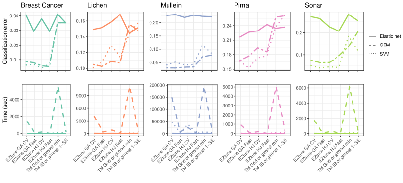
Figure 1: Classification errors and computation times for datasets with a binary response.

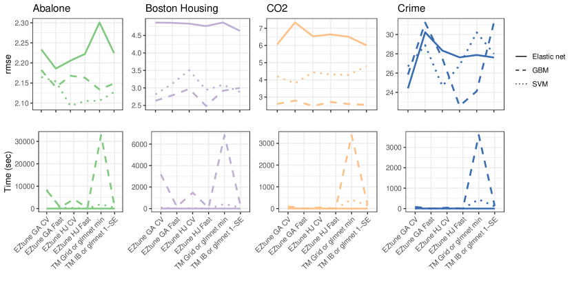
Figure 2: RMSEs and computation times for datasets with a continuous response.

6 Conclusions

Supervised learning models have the ability to increase prediction accuracy if they are tuned well, but tuning such models is not trivial. We discussed the advantages and disadvantages using caret, tidymodels, and EZtune for tuning such models. All of these packages are good options for tuning, but they each have strengths and weaknesses. Experienced R users may prefer the power and flexibility of caret, but that flexibility comes with the price of being difficult to learn and implement, even for experienced R users. Further, tidymodels is a good option for experienced R users who have a solid understanding of hyperparameters and wish to explore a larger set of statistical learning models. In contrast, EZtune is an excellent option for users who want fast and effective hyperparameter tuning for a smaller set of model types without the programming overhead required for other approaches. EZtune is a powerful tuning tool whose simple interface, ability to find a well tuned model, and fast computation time make it an excellent choice for general hyperparameter tuning or incorporation into a larger computational pipeline. Not only is EZtune an approachable option for someone new to statistical learning models, it is an excellent way to become familiar with statistical learning models and their hyperparameters. EZtune can be used to prepare users to interact with tidymodels and caret in the future if they choose to expand their choice of models.

References

- [1] R Core Team. R: A language and environment for statistical computing. R Foundation for Statistical Computing, Vienna, Austria, 2022.
- [2] Max Kuhn and Hadley Wickham. tidymodels: A collection of packages for modeling and machine learning using tidyverse principles, 2020.
- [3] Max Kuhn. caret: Classification and regression training, 2022. R package version 6.0-93.
- [4] Corinna Cortes and Vladimir Vapnik. Support-vector networks. Machine Learning, 20(3):273–297, 1995.
- [5] Jerome H. Friedman. Greedy function approximation: A gradient boosting machine. Annals of Statistics, pages 1189–1232, 2001.
- [6] Yoav Freund and Robert E. Schapire. A decision-theoretic generalization of on-line learning and an application to boosting. Journal of Computer and System Sciences, 55(1):119–139, 1997.
- [7] Hui Zou and Trevor Hastie. Regularization and variable selection via the elastic net. Journal of the royal statistical society: series B (statistical methodology), 67(2):301–320, 2005.
- [8] Jill F. Lundell. Tuning hyperparameters in supervised learning models and applications of statistical learning in genome-wide association studies with emphasis on heritability. PhD thesis, Utah State University, 2019.
- [9] Jerome Friedman, Trevor Hastie, and Robert Tibshirani. Regularization paths for generalized linear models via coordinate descent. Journal of Statistical Software, 33(1):1–22, 2010.
- [10] Chris Schumacher, Michael D. Vose, and L. Darrell Whitley. The no free lunch and problem description length. In Proceedings of the 3rd Annual Conference on Genetic and Evolutionary Computation, pages 565–570. Morgan Kaufmann Publishers Inc., 2001.
- [11] Alex J. Smola and Bernhard Schölkopf. A tutorial on support vector regression. Statistics and Computing, 14(3):199–222, 2004.
- [12] Trevor Hastie, Robert Tibshirani, and Jerome Friedman. The elements of statistical learning: Data mining, inference, and prediction. Springer, New York, NY, USA, 2009.
- [13] David Meyer, Evgenia Dimitriadou, Kurt Hornik, Andreas Weingessel, and Friedrich Leisch. e1071: Misc functions of the department of statistics, probability theory group (Formerly: E1071), TU Wien, 2022. R package version 1.7-12.
- [14] Joao Gama. Iterative bayes. Theoretical Computer Science, 292(2):417–430, 2003.
- [15] Loi Lei Lai and Tze Fun Chan. Distributed generation: Induction and permanent magnet generators. John Wiley & Sons, 2008.
- [16] D. Goldberg. Genetic algorithms in search optimization and machine learning. Addison-Wesley Longman Publishing Company, Boston, MA, USA, 1999.
- [17] Max Kuhn and Kjell Johnson. AppliedPredictiveModeling: Functions and data sets for applied predictive modeling, 2018. R package version 1.1-7.
- [18] David J Newman, SCLB Hettich, Cason L Blake, and Christopher J Merz. UCI repository of machine learning databases, 1998, 1998.
- [19] Shonda Kuiper and Jeffrey Sklar. Practicing statistics: Guided investigations for the second course. Pearson, Boston, MA, USA, 2013.
- [20] Hannah Frick, Fanny Chow, Max Kuhn, Michael Mahoney, Julia Silge, and Hadley Wickham. rsample: General resampling infrastructure, 2022. R package version 1.1.1.
- [21] Alexandros Karatzoglou, Alex Smola, and Kurt Hornik. kernlab : Kernel-based machine learning lab, 2022. R package version 0.9-31.
- [22] Tianqi Chen, Tong He, Michael Benesty, Vadim Khotilovich, Yuan Tang, Hyunsu Cho, Kailong Chen, Rory Mitchell, Ignacio Cano, Tianyi Zhou, Mu Li, Junyuan Xie, Min Lin, Yifeng Geng, and Yutian Li. xgboost: Extreme gradient boosting, 2022. R package version 1.6.0.1.
- [23] Brandon Greenwell, Bradley Boehmke, Jay Cunningham, and GBM Developers. gbm: Generalized Boosted Regression Models, 2022. R package version 2.1.8.1.