X-Shooting ULLYSES: Massive stars at low metallicity

Abstract

Context. The winds of massive stars have a significant impact on stellar evolution and on the surrounding medium. The maximum speed reached by these outflows, the terminal wind speed $v_{\infty}$, is a global wind parameter and an essential input for models of stellar atmospheres and feedback. With the arrival of the ULLYSES programme, a legacy UV spectroscopic survey with the Hubble Space Telescope, we have the opportunity to quantify the wind speeds of massive stars at sub-solar metallicity (in the Large and Small Magellanic Clouds, $0.5Z_{\odot}$ and $0.2Z_{\odot,}$ respectively) at an unprecedented scale.

Aims. We empirically quantify the wind speeds of a large sample of OB stars, including supergiants, giants, and dwarfs at sub-solar metallicity. Using these measurements, we investigate trends of $v_{\infty}$ with a number of fundamental stellar parameters, namely effective temperature ($T_{\rm{eff}}$), metallicity ($Z$), and surface escape velocity $v_{\mathrm{esc}}$.

Methods. We empirically determined $v_{\infty}$ for a sample of 149 OB stars in the Magellanic Clouds either by directly measuring the maximum velocity shift of the absorption component of the C IV $\lambda\lambda$1548-1550 line profile, or by fitting synthetic spectra produced using the Sobolev with exact integration method. Stellar parameters were either collected from the literature, obtained using spectral-type calibrations, or predicted from evolutionary models.

Results. We find strong trends of $v_{\infty}$ with $T_{\rm{eff}}$ and $v_{\mathrm{esc}}$ when the wind is strong enough to cause a saturated P Cygni profile in C IV $\lambda\lambda$1548-1550. We find evidence for a metallicity dependence on the terminal wind speed $v_{\infty}\propto Z^{0.22\pm 0.03}$ when we compared our results to previous Galactic studies.

Conclusions. Our results suggest that $T_{\rm{eff}}$ rather than $v_{\mathrm{esc}}$ should be used as a straightforward empirical prediction of $v_{\infty}$ and that the observed $Z$ dependence is steeper than suggested by earlier works.

1 Introduction

Hot, massive stars ($>8M_{\odot}$) are known to host radiatively driven outflows. The strong ultraviolet (UV) flux of these stars transfers enough momentum outward through scattering with or absorption by UV metal ion line transitions to remove material from the stellar surface (Lucy & Solomon 1970; Castor et al. 1975). These winds are an essential factor in the evolution of the star as they can reduce the stellar mass considerably throughout the stellar lifetime, thereby altering both the evolutionary pathway (Ekström et al. 2012) and the properties of the end products (Langer 2012; Smith 2014).

Typically, two fundamental global parameters are used to describe the winds of massive stars: the mass-loss rate ($\dot{M}$), and the asymptotic or terminal speed of the outflow ($v_{\infty}$) (Puls et al. 2008; Hillier 2020; Vink 2022). When the winds are adiabatic, the wind luminosity ($0.5\dot{M}v_{\infty}^{2}$) determines the efficiency of the wind feedback (Weaver et al. 1977). Ionising radiation from stars (Spitzer 1978; Dale et al. 2012) also plays an important role that often combines in non-linear ways with wind feedback (Geen & de Koter 2022).

Resonance transitions at UV wavelengths of species such as carbon are prime diagnostics of the terminal velocity, especially when the spectral lines remain optically thick at the distances where the wind velocity reaches $v_{\infty}$. The advantage of this is that the terminal wind speed can be measured directly from UV spectroscopy. This measurement is independent of all other stellar parameters because we observe an extended region of zero flux in the P Cygni profile of the resonance line, the farthest extent of which is associated with the maximum velocity of wind material available to block the emergent light (Prinja et al. 1990). We also observe a rapid increase from zero to continuum flux levels at the blue edge of the resonance-line profile. The gradient of the profile edge can be reduced through high-velocity turbulent gas generated by shocks coming from collisions between high-velocity low-density material and low-velocity high-density material and can be used to diagnose the characteristic velocity dispersion of the outflow. The formation of this multi-component wind is inherent to massive stars through the instability associated with radiation line-driving (MacGregor et al. 1979; Carlberg 1980; Owocki & Rybicki 1984; Feldmeier 1995; Driessen et al. 2019).

Absorption troughs of resonance-line profiles may not reach zero flux for all stars. For stars without P Cygni saturation, a wind speed can still be measured from the blue edge of the line profile, but it will then not reflect the terminal wind speed, but rather the maximum observed wind speed at the highest velocity of the absorption profile, or a lower limit to $v_{\infty}$. The wind speeds can also be measured by fitting simplified models, which implement the Sobolev with exact integration method (SEI) from Lamers et al. (1987), and are significantly less computationally expensive than full stellar atmosphere and wind models. There may be some offset between wind speeds that are directly measured from the trough and those obtained through fitting. By applying the SEI fitting method to all stars in the sample, we are able to quantify possible discrepancies between SEI and DM values and comment on the uncertainty of the terminal wind speeds from unsaturated resonance lines.

Line-driven wind theory predicts that the strength of stellar winds changes with metallicity (Puls et al. 2000), so there is a need to empirically quantify the wind strength in environments with metallicities different than that of the Milky Way. Theoretical (Vink et al. 2001; Krtička & Kubát 2018; Björklund et al. 2021) and empirical (Mokiem et al. 2007; Ramachandran et al. 2019) studies have been conducted to quantify the $\dot{M}(Z)$ dependence of OB stars. Empirical studies have shown that it is not straightforward to quantify the $v_{\infty}(Z)$ dependence with observations of massive stars that are currently available because while $v_{\infty}$ has been determined for 250 OB stars (Prinja et al. 1990), the parameter space coverage of stars at low metallicity with prominent, observable UV wind line profiles is limited (Haser 1995; Garcia et al. 2014; Marcolino et al. 2022). As a result of this, the only predictions of $v_{\infty}(Z)$ are theoretical (Leitherer et al. 1992; Krtička & Kubát 2018; Björklund et al. 2021; Vink & Sander 2021), with the most widely used prediction being $\sim{}Z^{0.13}$ from Leitherer et al. (1992). The Hubble Space Telescope (HST) UV Legacy Library of Young Stars as Essential Standards (ULLYSES; Roman-Duval et al. 2020) programme changes this situation, providing UV spectroscopy of a large sample of O, early-B, mid- to late-B supergiant and Wolf-Rayet type stars spanning the upper Hertzsprung-Russell diagram (HRD) in the Large and Small Magellanic Clouds (LMC and SMC). These two satellite galaxies represent environments with metallicities that are substantially lower than that of the Milky Way; the metallicity of the LMC is one-half and that of the SMC is one-fifth of the solar metallicity (Mokiem et al. 2007).

The opportunity arises with this dataset (if sufficient characterisation of the stars is available) to explore trends in the wind speed with fundamental stellar parameters, which might allow for future empirical predictions of the terminal wind speed given other fundamental stellar parameters such as the luminosity and effective temperature. This has been done for Galactic stars and is discussed throughout Sect. 5 (see e.g. Kudritzki & Puls 2000 and references therein). This could help to make a well-educated assumption for $v_{\infty}$ in stellar atmosphere studies that lack a $v_{\infty}$ diagnostic (Bouret et al. 2015). Conversely, these trends could be used to estimate stellar parameters from terminal wind speeds, allowing for calibrations of stellar parameters without extensive atmosphere modelling. This may only be useful when only $v_{\infty}$ is known, however, because a spectral type classification will likely give a better estimation of the stellar parameters. Here we present an analysis of the terminal wind speeds of a sample of 149 OB stars in the LMC and SMC by investigating trends with fundamental stellar parameters including effective temperature, surface escape speed, and metallicity.

The paper is laid out as follows: Section 2 introduces the ULLYSES sample and the associated UV observations obtained with the HST. Section 3 outlines our method for measuring wind speeds and obtaining or estimating other stellar parameters. In Section 4 we present the results of this analysis, including the terminal wind speeds. In Section 5 we discuss the relations between terminal wind speeds and other stellar parameters, and we compare them to similar studies in the Galaxy. Our conclusions are given in Section 6.

2 Sample and observations

The sample used in this work was obtained as part of the ULLYSES programme (Roman-Duval et al. 2020), which aims to secure high-quality UV spectra of massive stars in the LMC and SMC, sampling all spectral sub-types and luminosity classes from O2 to B1.5, as well as supergiants in the range of B2 to B9 with redundancy. This study uses spectra up to the third ULLYSES data release. This includes 67 stars in the LMC and 82 stars in the SMC. The LMC sample comprises 39 OB supergiants, 14 OB giants, and 14 OB dwarfs. The SMC sample includes 39 OB supergiants, 13 OB giants, and 30 OB dwarfs. The distribution of targets by spectral type and luminosity class is shown in Fig. 1. The full list of objects is presented in Tables 2 to 7.

2.1 UV data

The data were obtained with either the Cosmic Origins Spectrograph (COS) or with the Space Telescope Imaging Spectrograph (STIS), using the appropriate grating required to obtain sufficient coverage of relevant diagnostics, depending on the target spectral type. The target signal-to-noise ratio (S/N) differs slightly for each grating; generally, S/N $\approx$ 20-30. This essentially means that the bright targets are observed with STIS and the fainter stars are observed with COS, which offers better sensitivity at the cost of spectral resolution. The COS gratings cover the spectral range from 937 to 1792 Å for O2-O9 stars and 1830 to 2110 Å for B2-B9 stars; the STIS gratings run from 1141 to 2366 Å for O2-B9 stars and from 2275 to 3119 Å for B5-B9 stars (for which only supergiants were observed).

2.2 Stellar parameters

We adopted spectral types, luminosities, and effective temperatures from the ULLYSES metadata, comprised of both literature values and spectral type calibrations (Roman-Duval et al. (2020); full metadata are available on the ULLYSES website, latest access date: 5 April 2022). In order to estimate other stellar parameters, we compared luminosity and effective temperature to the single-star evolution models of Brott et al. (2011) and Köhler et al. (2015) with the Bayesian analysis tool BONNSAI (Schneider et al. 2014). This provides us with evolutionary masses and radii that allow us to compute the initial and current surface escape speeds,

$$v_{\rm{esc}}=(2\mathrm{G}M(1-\Gamma_{\rm{e}})/R)^{1/2},$$ (1)

where G is the gravitation constant, $M$ is the stellar mass, $R$ is the stellar radius, and $\Gamma_{\rm{e}}$ is the Eddington parameter: the ratio of radiative acceleration to local gravitational acceleration, here assuming the radiative component to be purely electron scattering. Throughout this paper, any mention of surface escape speed refers to surface escape speeds reduced by electron scattering, as defined here. We highlight there will be additional uncertainties on the escape speeds used here as stellar evolutionary tracks are shaped by a number of other stellar parameters, such as the rotational velocity and mass-loss rate, which will affect the BONNSAI results. For example, a reduction in mass-loss rate on the main sequence by a factor of 3 or more would introduce a systematic correctional shift to higher evolutionary masses. Moreover, stellar properties such as the mass and radius will vary when different stellar evolutionary codes are used (see e.g. Agrawal et al. 2021).

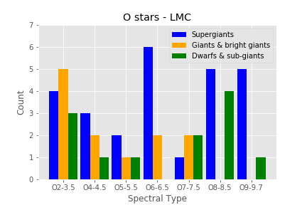
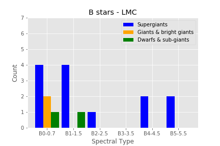
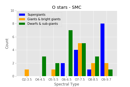
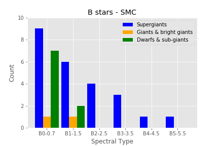
Figure 1: Histogram of the distribution of the stellar sample through spectral type and luminosity class. LMC stars are shown in the first and second panels, which correspond to the O- and B-type stars, respectively. Similarly, SMC stars are presented in the third and fourth panels.

3 Methods

We employed two methods to measure the terminal wind speeds. The initial method, direct measurement (DM), can be used for stars with saturated resonance-line profiles (Prinja et al. 1990). Direct measurement can also be applied to stars with unsaturated profiles, but then only a lower limit on $v_{\infty}$ can be obtained. The second method, SEI modelling, is needed for stars without saturation in their UV resonance-line profiles, although it can also be used for stars with saturated profiles (Lamers et al. 1987). SEI models are further needed to constrain the turbulent velocity of the wind ($v_{\rm{turb}}$). For either method, minimal data processing is required from the ULLYSES high-level science product spectra; only a local normalisation around the spectral line of interest was carried out.

A few caveats must be pointed out. We did not consider the radial velocity of individual stars when fitting the profiles because the lack of isolated absorption line profiles in the UV makes these measurements difficult. We only compensated for the radial velocity associated with the host Magellanic Cloud by applying a Doppler shift to our SEI model before comparing to the observed spectrum, 262 $\rm{km}\,\rm{s^{-1}}$ in the LMC, and 146 $\rm{km}\,\rm{s^{-1}}$ in SMC (McConnachie 2012). An optical follow-up survey with the X-Shooter spectrograph on the European Southern Observatory (ESO) Very Large Telescope (VLT), named X-Shooting ULLYSES (XShootU), will allow for radial velocity measurements that can be applied to the wind speeds afterwards (Vink et al. in prep.). In the meantime, we consider the impact of differences in radial velocity on our measurements of $v_{\infty}$ using preliminary radial velocity measurements for individual stars from the XShootU collaboration. Any necessary corrections due to stellar radial velocities are small because the largest deviations from the systemic velocity of the Cloud correspond to a shift of 100 $\rm{km}\,\rm{s^{-1}}$ in $v_{\infty}$. For the majority of the sample, the corrections are much smaller. Generally, any discrepancies in $v_{\infty}$ due to radial velocity are covered by our error estimates. There are also assumptions made in our SEI model, discussed in Section 3.2, that would cause issues if we attempted to fit the full P Cygni profile. These assumptions have little impact on our results here because we only examined a sub-section of the profile centred around the wavelength of the high-velocity edge of the absorption profile.

We did not check the spectra for signatures of binarity. While undetected companions are possible, they are likely to be of relatively low luminosity and so would only provide weak signatures in the spectra. Companions like this would have a negligible impact on the strong P Cygni wind profiles used in this study.

Several strong resonance profiles are located in the covered wavelength ranges: N v $\lambda\lambda$1239-1243, C iv $\lambda\lambda$1548-1551, and Si iv $\lambda\lambda$1394-1403 in the spectra of O- and early B-type stars, with C ii $\lambda\lambda$1335-1336 and Al iii $\lambda\lambda$1855-1863 appearing in the spectra of B0.7-B2 Ia stars. Unfortunately, the N v line is strongly blended by interstellar Ly$\alpha$ absorption. The separation of the doublet lines in Si iv is 9 Å or 1930 km s^-1. This complicates a reliable determination of the terminal flow speed from the methods applied in this study. As the C ii and Al iii resonance lines appear in only a few stars, we limited our diagnostic in the present work to the strong C iv doublet. The C iv $\lambda\lambda$1548-1551 doublet used in this study is commonly saturated and is therefore a good and consistent diagnostic throughout the ULLYSES sample, but it is also possible to determine terminal wind speeds through other methods and diagnostics, which can be focused on in future studies. For example, a significant number of stars are complemented by archival observations made with the Far Ultraviolet Spectroscopic Explorer (FUSE), including additional diagnostics such as P v 1118-1128 and C iii 977, which may also show saturated or strong P Cygni profiles. Additionally, narrow absorption components (NACs) have been shown to be a good indicator of the terminal wind speed (e.g. Prinja et al. 1990), and a number of well-defined NACs can be seen throughout the ULLYSES spectra.

3.1 Direct measurement

The DM method is facilitated by the fact that for line profiles with extended saturation, the terminal wind speed can be measured directly. We did this by measuring the wavelength of the bluest edge of the P Cygni absorption trough showing zero flux, as established in Prinja et al. (1990). Given the S/N of the observed spectra, discussed in Sect. 2, it can be illustrative to measure the wavelength of minimum absorption within the boundaries of flux variation allowed by the S/N. This velocity of minimum absorption deviates from the directly measured terminal wind speed by 60 km s^-1 on average, but can be as high as 200 km s^-1. Examples of the velocity of minimum absorption can be seen in the lower panels of Fig. 2, which show unsaturated line profiles. The difference between these two measurements is provided as the error on a directly measured terminal wind speed for a saturated profile. We took 100 km s^-1 as a conservative estimate on the uncertainty of the lower limit of the terminal wind speed found from non-saturated line profiles using the DM method.

3.2 SEI modelling

If the C iv $\lambda\lambda$1548-1551 doublet is not saturated, the method used to constrain the wind speed is to reproduce this profile with synthetic spectra. This modelling can be made at relatively low computational expense, using the Sobolev with Exact Integration (SEI) method first developed by Lamers et al. (1987). The SEI code applied in this work builds on the code of Haser et al. (1995) and is presented in Sundqvist et al. (2014). In short, the method combines a computation of the source function with the Sobolev (1960) escape probability method with a formal solution of the radiative transfer equation. The radial distribution of the opacity (or number density) of the ionisation species at hand is parametrised, including chaotic small-scale motions in the flow that cause clumping and porosity effects in both physical and velocity space. We did not use these velocity-porosity modifications because we are only interested in constraining $v_{\infty}$ and $v_{\rm{turb}}$. As we do not aim to reproduce the full morphology of the profile, we limited our input free parameters. We fixed the $\beta$ wind acceleration parameter to unity. This choice impacts the profile morphology close to the line centre, but this region is not assessed in our fit evaluation. We varied only four parameters: the terminal wind speed, the microturbulent velocity $v_{\rm{turb}}$ , and two parameters ($\kappa{}_{0}$ and $\alpha$) describing the line opacity. The latter is formalised as

$$\kappa(v)=\kappa_{0}\left(\frac{v}{v_{\infty}}\right)^{\alpha},$$ (2)

where $\kappa{}_{0}$ is a dimensionless opacity parameter (Hamann 1981). $\kappa{}_{0}$ and $\alpha$ were varied to match the strength of the absorption, therefore their magnitudes are not necessarily physically motivated. However, the turbulent wind speed can be constrained with the gradient of the return to continuum from the high-velocity edge of the absorption profile, and this parameter will affect the terminal wind speed. Generally, we aimed to fit the full blue edge, including this gradient. This means that the wind turbulence included in the SEI model adds to the overall wind speed and $v_{\infty}$ is reduced to compensate for this. As a result, $v_{\infty}$(SEI) is usually lower, causing the difference between $v_{\infty}$(SEI) and $v_{\infty}$(DM). Including this (often supersonic) turbulence in the SEI model essentially acts as broadening the profile function, but this has a similar effect on the emergent line profile as a more physically motivated simulation in terms of multiple non-monotonic velocity fields (shock structure), as suggested by Lucy (1982) and Lucy (1983) (see also Puls et al. 1993). The difference between $v_{\infty}$ as derived from $v_{\infty}$(DM) or from $v_{\infty}$(SEI) also depends on the strength of the line (which is proportional to the wind strength). If the strength is not too large (but large enough to saturate), the broadening by the large $v_{\rm{turb}}$ will not play a very strong role, and the difference will be small. However, when the strength is (very) large, the profile function can contribute also from regions that lie quite far away from line centre, and $v_{\infty}$(DM) becomes larger than $v_{\infty}$(SEI). This is somewhat different compared to a simulation using the wind-shock structure because in the latter case, the high-velocity regime is usually quite thin, so that its contribution remains more limited (unless the high-velocity interclump material is not as thin as usually adopted, see Zsargo et al. 2008; Hawcroft et al. 2021; Brands et al. 2022). The SEI model is optimised using an optimisation routine (curve fit from the SciPy package, Virtanen et al. 2020) based on the Levenberg-Marquardt evaluation criteria. The statistical error from this fitting routine is the $v_{\infty}$(SEI) uncertainty listed in Tables 2 to 7.

4 Results

In this section, we present our measured terminal wind speeds along with stellar parameters from the ULLYSES metadata. Some subjective quality assessment was made during this analysis in order to eliminate stars for which the measurement of the terminal wind speed is unreliable because we did not observe the true terminal wind speed. The profiles are ranked by reliability to determine a terminal wind speed, with a poorer ranking given to stars that either have relatively low S/N spectra in the region of interest or that lack significant wind signatures. The categories are as follows:

1. Best quality: Clear and extended (¿1Å) saturation in the C iv $\lambda\lambda$1548-1551 profile.

2. Good quality: Strong wind signature, showing either a small saturation region or a significant absorption trough, ¿1Å of minimum flux is below the level of half the continuum.

3. Poor quality: Weak wind signature, trough is not significantly separated from continuum (minimum flux is above half of continuum average).

4. Worst quality: No estimate of the wind speed can be made either due to data quality or lack of wind signature.

Examples of line profiles for each category are shown in Figure 2.

In the end, the sample yields 37 stars in the LMC and 16 in the SMC with saturated profiles fulfilling our highest-quality measurement criteria (rank i). This sub-sample was used to measure robust trends with escape speed, temperature, and metallicity, which are presented in Sections 5.1 to 5.3. The larger sample is also considered and discussed in Appendix B.

We list all measurements of terminal wind speed in Tables 2 to 7. When the terminal wind speeds are both measured directly (denoted by $v_{\infty}$(DM)) and using SEI fitting ($v_{\infty}$(SEI)), they generally agree well with each other (Fig. 3). In terminal wind speed measurements of saturated profiles (best-quality rank, green circles in Fig. 3), we find a systematic offset between $v_{\infty}$(SEI) and $v_{\infty}$(DM) because the addition of turbulence reduces $v_{\infty}$(SEI). However, this offset shift occurs more often in the LMC, which may be evidence of the effect discussed in Sect. 3.2, where in the LMC (higher wind densities), the majority of the saturated lines (in green) provide a $v_{\infty}$(DM) ¿ $v_{\infty}$(SEI) because of a non-negligible influence of the high-velocity material. This effect would more or less vanish in the SMC because the high-velocity components affect the SMC less because of the lower wind densities. An opposing offset is present in measurements of the maximum observable wind speed in unsaturated profiles (lower quality rank, e.g. blue triangles in Fig. 3); there are more stochastic discrepancies between the two methods on a case-by-case basis, with indeed some very large discrepancies in lower-quality measurements. For some stars, the point of minimum flux in the profile may be far enough from the blue edge that even within the S/N limit, the edge of the profile is not included in a direct measurement. This means that the offset occurs in the opposite direction ($v_{\infty}$(SEI) ¿ $v_{\infty}$(DM)), as the SEI method attempts to fit the blue edge, which is excluded by direct measurement. The profile of AV26, shown in the second panel of Fig. 2, is an example of this, and the overall trend is clearest in the blue triangles in Fig. 3.

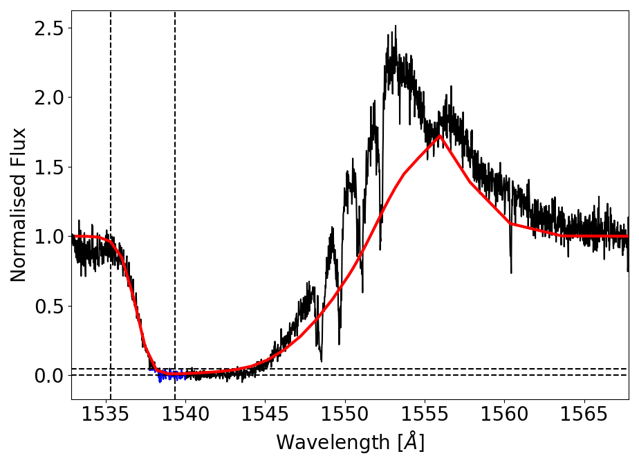
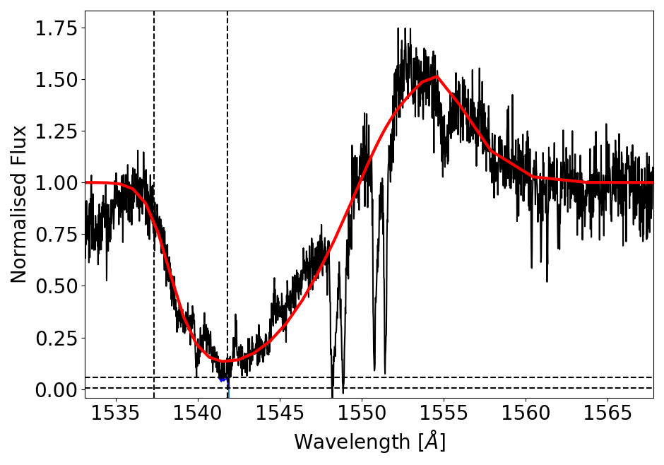
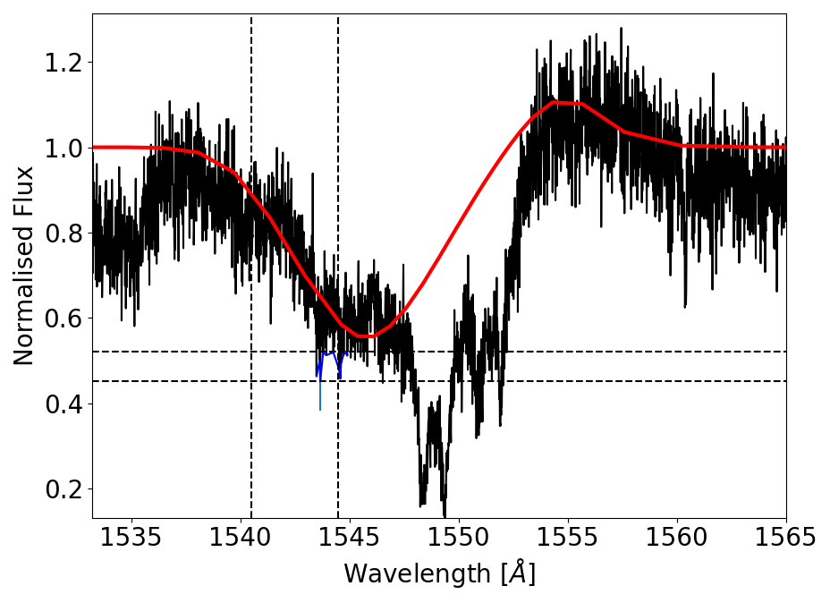
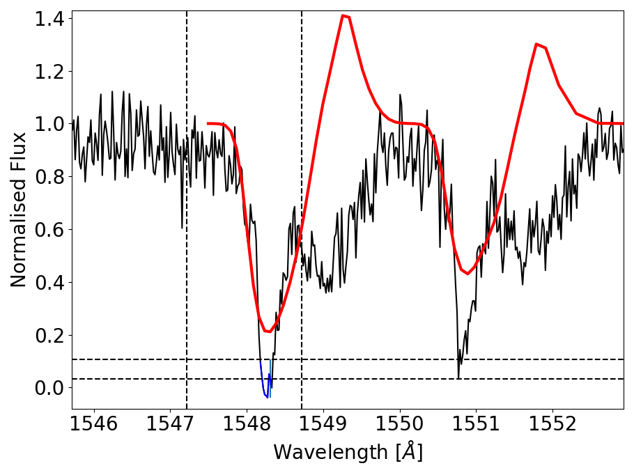
Figure 2: Example of C iv $\lambda\lambda$1548-1550 line profiles for different reliability categories from highest (top panel, rank i) to lowest (bottom panel, rank iv). Two profiles shown in this figure are from LMC stars (Sk –65^∘ 47 and Sk –71^∘ 19), and two are from SMC stars (AzV 26 and AzV 216) from the highest to the lowest panel: Sk –65^∘ 47(O4If), AzV 26 (O6If), Sk –71^∘ 19 (O6III), and AzV 216 (B1III). Black lines are the observed spectra. Red lines are the best-fit SEI model. Vertical dashed black lines highlight the fitting region for the SEI model. Horizontal dashed black lines show the S/N limit on the minimum flux of 0. Blue lines are the minimum flux within the S/N.

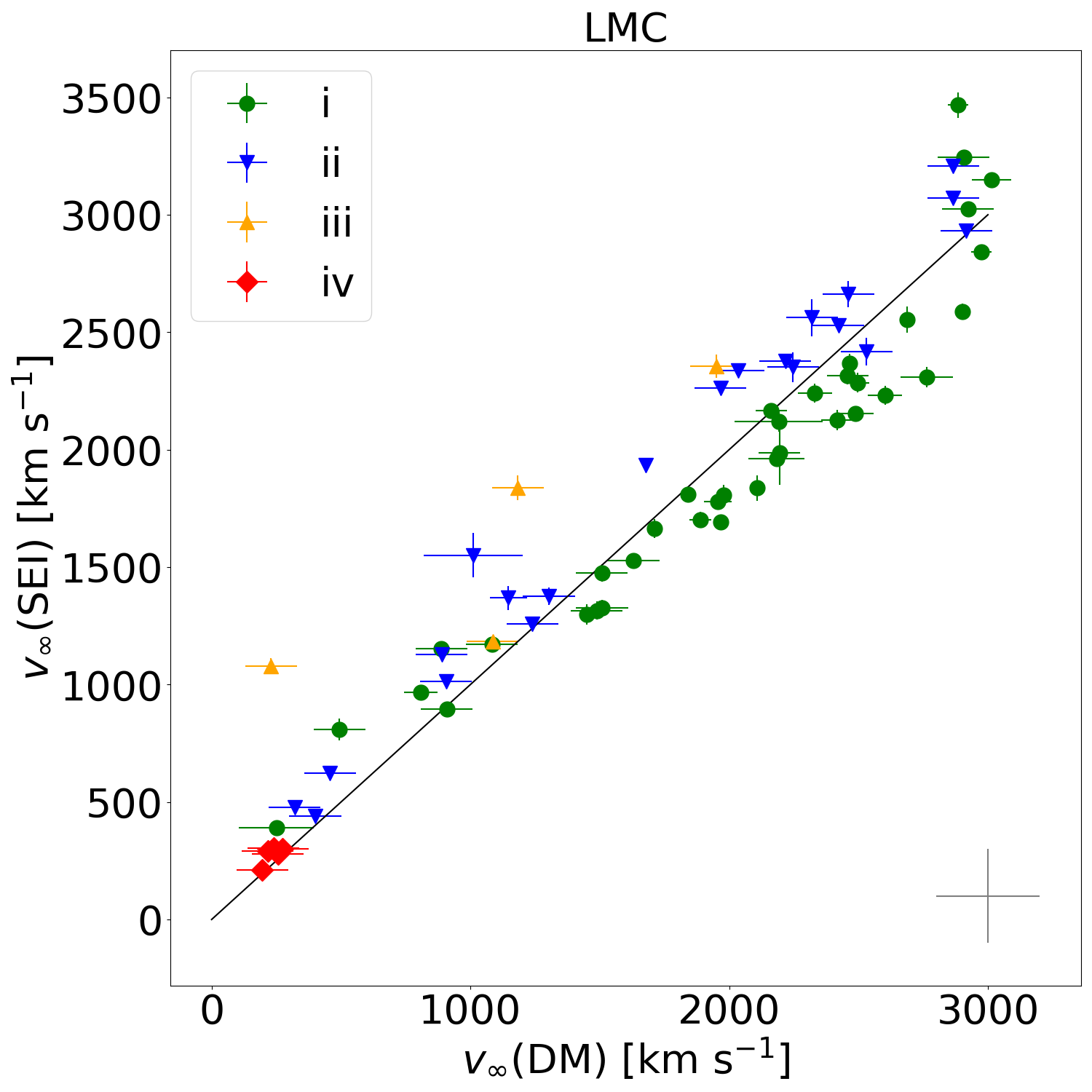
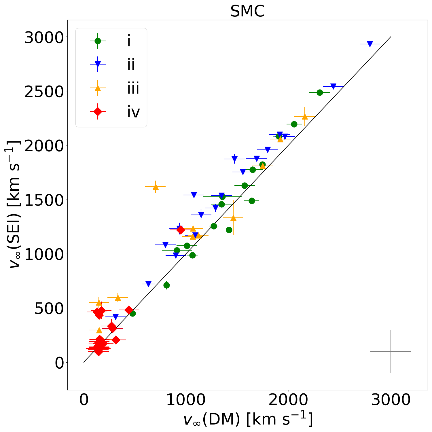
Figure 3: Comparison between terminal wind speed found using direct measurement $v_{\infty}$(DM), against that found using the SEI method $v_{\infty}$(SEI). Upper panel: LMC sample. Lower panel: SMC sample. Symbol shapes and colours indicate different quality categories from best (i) to worst (iv) (see the legend and Sect. 4). The solid black line is a one-to-one relation between $v_{\infty}$(DM) and $v_{\infty}$(SEI). Conservative uncertainties of 200 $\rm{km}\,\rm{s^{-1}}$ on each measurement are visualised through the grey cross in the lower right corner of each panel.

Statistical errors on $v_{\infty}$(SEI) come from our optimisation routine. A more realistic precision for $v_{\infty}$(SEI) is to consider our values accurate to within 100 or 200 $\rm{km}\,\rm{s^{-1}}$ to account for the effect of wind turbulence on the measurement of $v_{\infty}$(SEI). As discussed in Sect. 3.2, the stronger the effect of turbulence, the larger the uncertainty on $v_{\infty}$.

5 Discussion

In this section, we explore the trends of the terminal wind speed with fundamental stellar parameters. The terminal wind speeds used here are those measured using the SEI method. We find that the differences between terminal wind speeds obtained using SEI or DM are not significant or systematic enough to affect these trends or conclusions. We also compare these trends with previous observational studies and applicable theoretical predictions.

The linear trends were assessed with orthogonal distance regression (ODR), taking the errors on both variables into account, with an optimisation routine from the SciPy package applied to the relevant function (Virtanen et al. 2020). For this discussion, we focus on the stars that fulfill our highest-quality measurement criteria. Further discussion is included in Appendix B. We expect some intrinsic scatter on the linear relations due to variability in the winds resulting from the line-deshadowing instability. There will also be scatter, especially at low Z, when different combinations of CNO abundances are accounted for because the outer wind is driven by only a few dozen metal lines (e.g. C, N, and O; see, e.g. Krtička 2006; Puls et al. 2008).

5.1 $v_{\infty}\>$ vs $\>v_{\rm{esc}}$

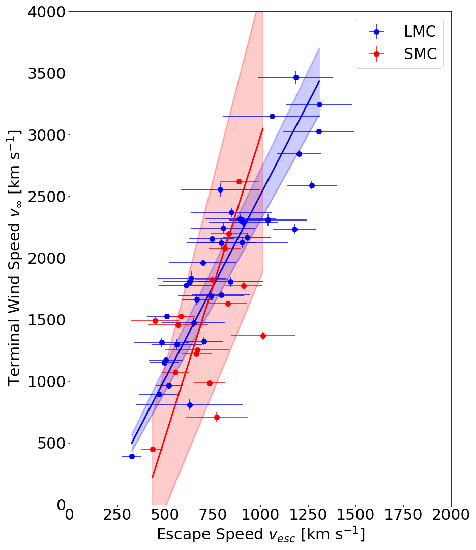
Figure 4: Terminal wind speed vs escape speed for LMC and SMC stars, shown in blue and red, respectively. Terminal wind speeds are measured by fitting SEI models to spectra, and the effective temperature estimates are acquired either through spectral type calibrations or from the literature. Escape speeds are estimated using evolutionary models computed with BONNSAI, given input stellar parameters from the literature or spectral type calibrations.

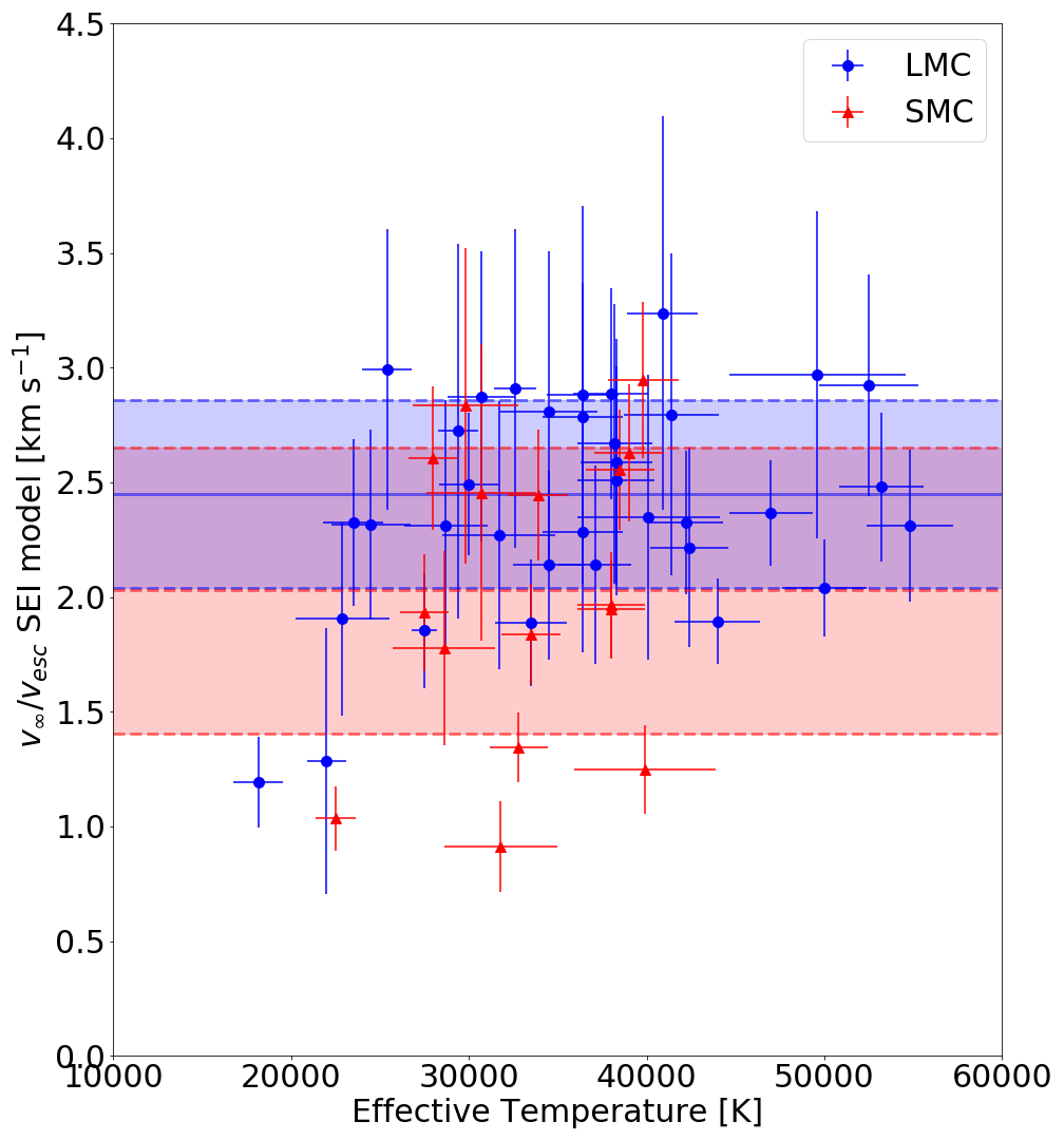
Figure 5: Ratio of the terminal wind speed to the escape speed vs effective temperature for LMC and SMC stars, shown in blue and red, respectively. The terminal wind speeds measured by fitting SEI models to spectra, and the effective temperature estimates are acquired either through spectral type calibrations or from literature.

The terminal wind speed has been predicted to follow strong relations with the surface escape velocity. A straightforward scaling with escape speed is predicted from radiation line driven wind theory, of the form $v_{\infty}=2.25(\alpha/(1-\alpha))v_{\rm{esc}}$ , where $\alpha$ is the main line force multiplier parameter (Kudritzki et al. 1989; Kudritzki & Puls 2000). The most commonly implemented scaling is a constant $v_{\infty}=2.65v_{\rm{esc}}$ that comes from the combination of a number of observational studies (Howarth & Prinja 1989; Prinja et al. 1990; Lamers et al. 1995; Howarth et al. 1997; Prinja & Crowther 1998; Puls et al. 1996; Kudritzki et al. 1999), compiled in Kudritzki & Puls (2000). This scaling was found to apply only at temperatures above 21 kK, and to decrease at lower temperatures. Temperature effects are discussed in the next sub-section. This decrease initially appeared as a step down to another constant (Lamers et al. 1995), and was interpreted as a bistability (Pauldrach & Puls 1990), attributed to a change in ionisation balance (Vink et al. 1999). Further empirical studies suggest a more gradual decrease (Evans et al. 2004; Crowther et al. 2006). Markova & Puls (2008) compiled a number of observational studies, along with new measurements, to investigate this trend, and again found a gradual decrease down to roughly 13 kK. Below this point, any estimates of the terminal wind speed are highly uncertain due to a lack of observations of necessary diagnostics. Our sample contains only a few objects with an effective temperature lower than 25 kK. Thus, we cannot contribute to this discussion here.

The relation we find between the terminal wind speed and the escape speed for the LMC is

$$v_{\infty}=(3.0\pm 0.2)v_{\rm{esc}}-(470\pm 150),RMS=351\>\rm{km\,s}^{-1}.$$ (3)

This gradient is close to the relation of Kudritzki & Puls (2000), based on empirical studies of Galactic objects, and with relatively low scatter. For the SMC, we have

$$v_{\infty}=(4.9\pm 1.1)v_{\rm{esc}}-(1900\pm 780),RMS=700\>\rm{km\,s}^{-1},$$ (4)

although here the scatter is large. Relations between terminal wind speed and surface escape speed in the LMC and SMC are shown in Fig. 4.

We find average values of $v_{\infty}/v_{esc}(LMC)=2.4\pm 0.4$ and $v_{\infty}/v_{esc}(SMC)=2.0\pm 0.6$. The ratio of wind speeds is shown as a function of effective temperature in Fig. 5. These values agree well with the empirical Galactic ratio of terminal wind to escape speed from Kudritzki & Puls 2000, corrected for our predicted reduction in wind speed with metallicity (discussed further in Sect. 5.3). Krtička (2006) and Evans et al. (2004) find $v_{\infty}/v_{esc}=2.3$ and $v_{\infty}/v_{esc}=2.63$ for samples at SMC metallicity, respectively. The ratio from Evans et al. (2004) is determined empirically, while Krtička (2006) used a combination of theoretical predictions and empirical determinations. Markova & Puls (2008) find $v_{\infty}/v_{esc}=3.3\pm 0.7$ from stellar atmosphere fitting of a sample of Galactic supergiants with effective temperatures above 23 kK. Considering the large scatter and exclusion of lower values in the region between 21 kK and 23 kK, this is not a large disagreement with other estimates. Björklund et al. (2021) predicted a ratio higher than empirical studies with large scatter of $v_{\infty}/v_{esc}=3.3\pm 0.8$ for their Galactic models. These authors also find a strong trend of a decreasing ratio with increasing luminosity. Muijres et al. (2012) predicted a decreasing ratio with increasing temperature in their models with averages of $v_{\infty}/v_{esc}$ in a range from 3.1 to 3.6, depending on the modelling technique. However, theoretical predictions of $v_{\infty}/v_{esc}$ only extend to lower temperature limits of around 28 kK (Muijres et al. 2012; Björklund et al. 2021). If there is a flattening of the empirical $v_{\infty}/v_{esc}$ relation above this temperature (which could be argued from Fig. 5), then the theoretical and observational temperature dependences could converge at high temperatures and diverge mainly at lower temperatures. To resolve this, more measurements and predictions of $v_{\infty}$ for stars with temperatures below 28 kK are required, which could be tested against the predictions for B supergiants from Krtička et al. (2021).

It is unclear whether the theoretical predictions of $v_{\infty}/v_{esc}$ (e.g. Björklund et al. 2021, Muijres et al. 2012) are truly larger than observational findings (e.g. Kudritzki & Puls 2000) because the parameter ranges of the two techniques do not fully overlap. However, it is possible that $v_{\infty}$ is overestimated in models because physical processes that serve to alter the acceleration of the outer wind are underestimated. Some studies suggested that low-density winds are hotter on average because radiative cooling is inefficient, such that metals are present in the bulk wind at higher ionisation states (Lucy 2012; Lagae et al. 2021). This would reduce the radiation force and lower the terminal wind speeds in stellar wind models. Moreover, the opposite effect would occur observationally, and we would not see strong wind lines in the typical ionisation states. Therefore, we would find (artificially) low terminal wind speeds in the usual diagnostics. This could explain a number of our quality rank iv measurements of $v_{\infty}$. It may also be that the evolutionary masses used in empirical studies are systematically overestimated (Herrero et al. 1992).

5.2 $v_{\infty}\>$ versus $\>T_{\rm{eff}}$

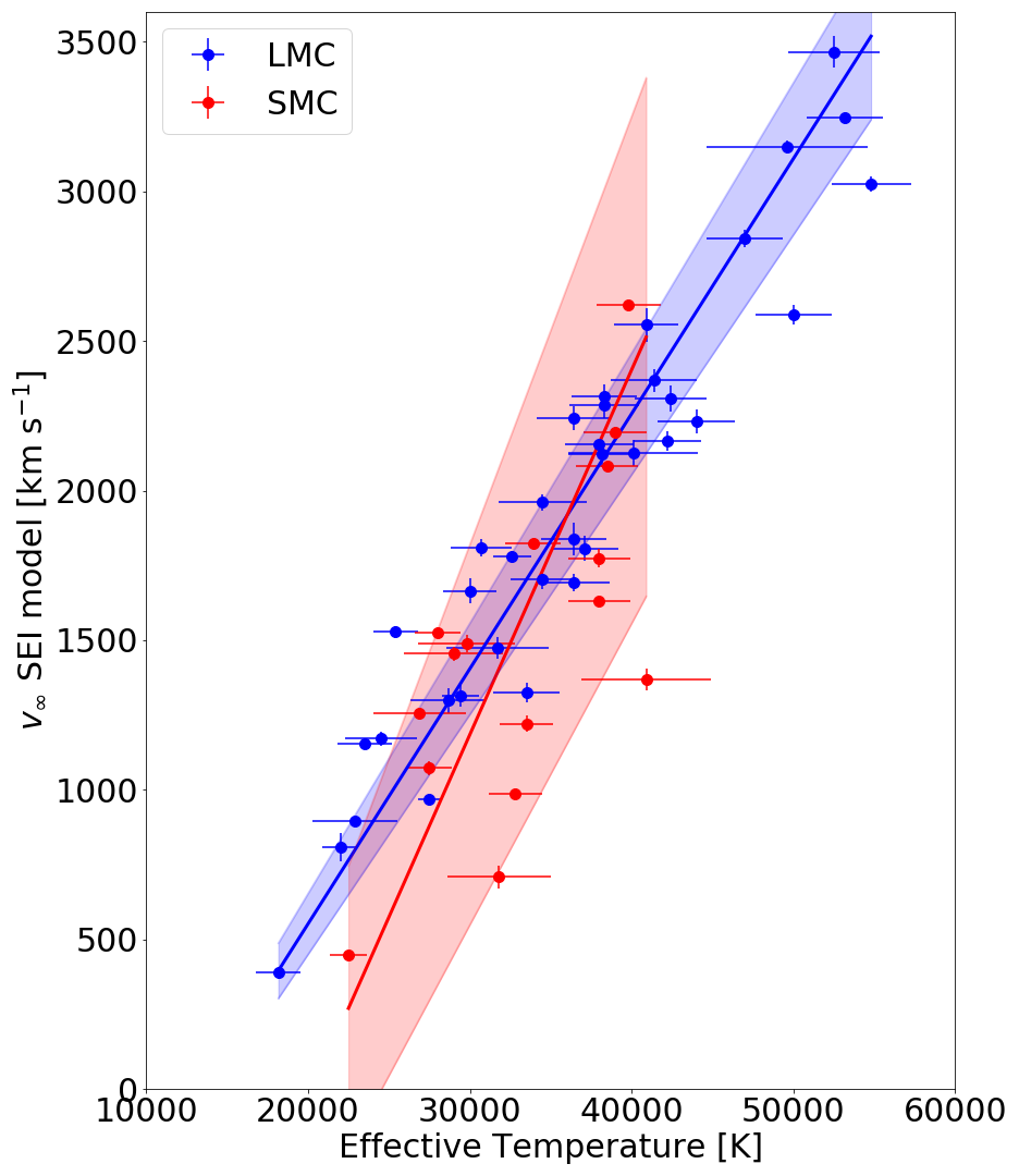
Figure 6: Terminal wind speed vs effective temperature for LMC and SMC stars, shown in blue and red, respectively. The terminal wind speeds are measured by fitting SEI models to spectra, and the effective temperature estimates are acquired either through spectral type calibrations or from the literature.

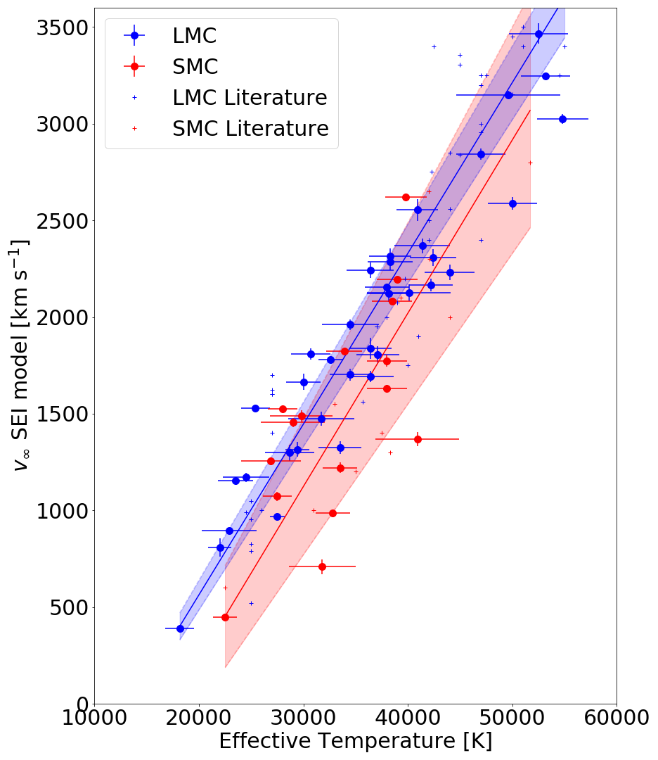
Figure 7: As Fig. 6, but including high-quality measurements of $v_{\infty}$ previously reported in the literature.

Table 1: ODR fit coefficients to relations between $v_{\infty}$ and $T_{\rm{eff}}$ as described in Eq. 5.

Region	a	b	RMS	Sample
	[$10^{-2}$]	[$\rm{km}\,\rm{s^{-1}}$]	[$\rm{km}\,\rm{s^{-1}}$]
LMC	$8.5\pm 0.5$	$1150\pm 170$	237	1
SMC	$12.2\pm 2.1$	$2470\pm 680$	477	1
LMC	$8.8\pm 0.4$	$1200\pm 150$	312	1,2
SMC	$8.9\pm 1.1$	$1560\pm 420$	372	1,2
GAL	$10.2\pm 0.3$	$1300\pm 100$	277	2

• The column ’sample’ indicates whether the fit is based on data from this paper (1) or from the literature (2), or both (1,2). The column ’RMS’ refers to the root mean square error.

We find a clear trend of increasing terminal wind speed with effective temperature. This is shown in Fig. 6 with linear fits of the form

$$v_{\infty}=aT_{\rm{eff}}-b.$$ (5)

The fit coefficients for different sub-samples are presented in Table 1. This general trend is well established, but it is most commonly tied to the escape speed, with which there is also a clear trend, but with slightly larger scatter. Considering the RMS of fits against both parameters, and that the known uncertainties in determining stellar masses and radii are larger than those on temperature, perhaps a more accurate empirical prediction of the terminal wind speed can be made using effective temperature rather than escape speed.

For the SMC, the trend with effective temperature shows a larger dispersion, spanning a limited range of 22-40 kK in temperature. However, the sample comprises only 16 stars, less than half of the equivalent LMC sample. As a result, the uncertainty is much larger than that found for the LMC. We can double the sample size by including stars from ULLYSES with slightly lower quality measurements (see Appendix B). However, only a few points are added above 40 kK when these stars are included, and we do not measure the true terminal wind speed, only a lower limit. We also find different slopes with much higher RMS when we include lower quality measurements in the LMC sample, which suggests that the trends found using these measurements are less reliable.

The temperature coverage in the SMC can be extended by adding equally high-quality measurements from literature samples compiled in Garcia et al. (2014), and additional measurements from Bouret et al. (2021). The high temperature coverage is provided by essentially one star (NGC346 MPG 355) that is included in the ULLYSES sample, but does not show saturation in the C iv $\lambda\lambda$1548-1551 and so is not included in our highest-quality rank sub-sample. However, this star does show saturation in the N v $\lambda\lambda$1239-1243 profile, which is fitted in Bouret et al. (2021), therefore we chose to include this literature measurement. Furthermore, the measured terminal wind speeds for this star in this work and Bouret et al. (2021) agree to within 150 km s^-1. Adding literature values from Garcia et al. (2014) to the LMC sample does not significantly impact the slope. This suggests that adding literature values for the SMC should serve only to reduce the uncertainty on our trend as the literature values add coverage at high effective temperature. When considering the literature sample of the SMC, we find a gradient similar to the LMC. The effect of including literature values is shown in Fig. 7. We note that the majority of the stars included in the highest-quality ranks, and so used to determine these relations, are supergiants. For example, in Fig. 6, the LMC sample comprises 70% luminosity class I stars, 20% class II-III and 10% class V. This means that these results mainly apply to stars with denser winds.

We may find a physical motivation of the dependence of the terminal wind speed on temperature by considering the mass-luminosity relation. As discussed in Sect. 5.1, we expect $v_{\infty}\propto v_{\rm{esc}}$ and $v_{\rm{esc}}\propto(M/R)^{0.5}$ , as shown in Eqn. 1. Using these relations and a mass-luminosity relation of the nature $L\propto M^{\alpha}$, we find $v_{\infty}\propto v_{\rm{esc}}\propto(L^{1/\alpha}/R)^{0.5}$. If we then substitute the luminosity for the Stefan-Boltzmann law ($L\propto R^{2}T_{\rm{eff}}^{4}$), we find that $v_{\infty}\propto((R^{2}T^{4})^{1/\alpha}/R)^{0.5}$. This results in a relation between terminal wind speed and temperature that becomes linear ($v_{\infty}\propto T_{\rm{eff}}$) when $\alpha\sim 2$. This offers some qualitative evidence for a relation of the terminal wind speed and temperature, although it is thought that the $\alpha$ exponent is slightly larger for more massive stars (Eker et al. 2015 find $\alpha\sim 2.7$ for main-sequence stars between 7 and 32 $M_{\odot}$).

5.3 $v_{\infty}\>$ versus $\>Z$

Leitherer et al. (1992) offered a theoretical power-law index for the terminal wind speed of the form $v_{\infty}\propto Z^{0.13}$ considering radiative transfer models of massive stars ($>15\,M_{\odot{}}$) covering a wide metallicity range $0.01\,Z_{\odot}\leq Z<3.0\,Z_{\odot}$. This dependence becomes $v_{\infty}\propto Z^{0.15}$ when the $Z$ range is restricted to $0.1\,Z_{\odot}\leq Z<3.0\,Z_{\odot}$. Further theoretical predictions for $v_{\infty}$ come from Krtička (2006), Vink & Sander (2021) and Björklund et al. (2021). Krtička (2006) offered the relation $v_{\infty}\sim Z^{0.06}$, although this prediction comes from comparing around 20 theoretical models at two metallicity points, $Z=0.2\,Z_{\odot}$ and $Z=0.3\,Z_{\odot}$. Using the Monte Carlo approach from Müller & Vink (2008) to predict terminal velocities and mass-loss rates, Vink & Sander (2021) obtained $v_{\infty}\propto Z^{0.19}$ for $0.033\,Z_{\odot}\leq Z<3\,Z_{\odot}$. Björklund et al. (2021) predicted $v_{\infty}\propto Z^{-0.10\pm 0.18}$. However, these authors also discussed issues with their predictions of terminal wind speed. We note further that these are average values. Björklund et al. (2021) reported that the $v_{\infty}/v_{esc}$ dependence is affected by the luminosity of stars considered, which also affects the metallicity dependence. The metallicity dependence of $v_{\infty}$ has been investigated empirically by Garcia et al. (2014). Their study included stars in the Galaxy, M31, M33, LMC, and SMC by compiling a number of studies that were then compared and extended further to IC 1613, which is suggested to have a very low metallicity ($\leq 0.1\,Z_{\odot}$). Altogether, these authors suggest a more complex metallicity dependence. For this study, we did not include M31, M33, or IC 1613 because the sample sizes are small, but we searched through the literature for $v_{\infty}$ measurements at Galactic metallicity.

We found a suitable Galactic sample from the stars with saturated wind line profiles in Prinja et al. (1990). In that paper, spectral types were determined or taken from previous references, and stellar parameters come from spectral type calibrations in Howarth & Prinja (1989). We used the measurements of $v_{\infty}$ from Prinja et al. (1990), but we used the stellar parameters from Holgado et al. (2020). Approximately 95% of the stars with saturated C iv $\lambda\lambda$1548-1551 profiles from Prinja et al. (1990) are included in Holgado et al. (2020). The stellar parameters of 70% of these stars were determined with quantitative spectroscopy, the others are identified as double-lined spectroscopic binaries, and Holgado et al. (2020) therefore did not present spectroscopic fits to these stars. We use this sub-sample of 66 stars with measurements of $v_{\infty}$ from Prinja et al. (1990) and effective temperatures from Holgado et al. (2020) in this section. In Appendix D we use the full Prinja et al. (1990) sample by updating spectral types using the Galactic O Star Spectroscopic Survey (GOSSS; Sota et al. 2011, 2014; Maíz Apellániz et al. 2016 and using these types to determine stellar parameters from the calibrations of Martins et al. (2005). We do not find a significant difference in the terminal wind speed with metallicity dependence for either Galactic sub-sample. There are also a number of B supergiants in the Prinja sample; these stars have no equivalent catalogue, therefore we confirmed the spectral types against various literature sources and updated them when the spectral type was revised in the subsequent literature. To determine stellar parameters for these stars, we used the spectral type calibration from McEvoy et al. (2015), who used Crowther et al. (2006) in the Galaxy. For the few B giants and dwarfs, we used the calibration of Dufton et al. (2006). The caveat then is that the effective temperatures for B stars in the relation still come from spectral type calibrations and could cause a systematic offset between the temperatures of the B and O stars. The consistency between B supergiant temperature calibrations from Markova & Puls (2008) (which agree very well with those from Crowther et al. 2006) and O star parameters, either from Martins et al. (2005) calibrations or Holgado et al. (2020), has been quantified by Berlanas et al. (2018). These authors concluded that the Holgado et al. (2020) parameters are preferred because the Martins et al. (2005) calibrations give low effective temperatures for late-O stars. This is also discussed in Simón-Díaz & Herrero (2014). Therefore, we also chose to use the O star parameters from Holgado et al. (2020) over the calibrations from Martins et al. (2005). We did not separate the sample into luminosity class in this section, but the effect of doing this is minimal. Therefore, the breakdown by luminosity class is presented in Appendix C. The effect of including other Galactic samples (Groenewegen et al. 1989; Crowther et al. 2006) is minimal and is presented in Appendix D.

To quantify the relation between $v_{\infty}$ and metallicity, we combined the highest-quality measurements in the Galaxy, LMC, and SMC, along with the appropriate LMC and SMC literature measurements discussed in Sect. 5.2, and applied a multi-dimensional linear fit to $v_{\infty}$ as a function of $T_{\rm{eff}}$ and $Z$. This yielded

$$v_{\infty}=\left[9.2(\pm 0.3)10^{-2}T_{\rm{eff}}-1040(\pm 100)\right]Z^{(0.22\pm 0.03)},$$ (6)

giving a final dependence of terminal wind speed on metallicity of the form $v_{\infty}\propto Z^{0.22\pm 0.03}$. With an $RMS=305$ km s^-1, we are able to reliably predict $v_{\infty}$ within a reasonable margin, offering an improvement on the uncertainty in stellar atmosphere and feedback modelling when $v_{\infty}$ diagnostics are unavailable. The relation between terminal wind speed and effective temperature for the Galaxy, LMC, and SMC is shown in Fig. 8.

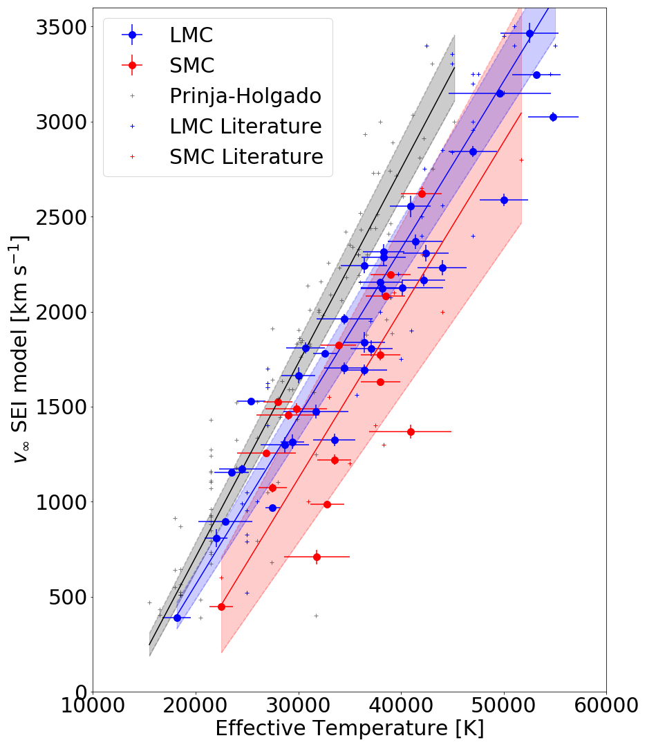
Figure 8: As Figure 6, but including the literature sample for Galactic OB stars to illustrate the metallicity dependence of the terminal wind speed.

6 Conclusions

We have empirically determined the terminal wind speeds for all OB type stars in the ULLYSES Data Release 3 sample. For stars with saturated C IV $\lambda\lambda$1148-1150 line profiles, we directly measured the terminal wind speed. For those with unsaturated C IV $\lambda\lambda$1148-1150 profiles, we measured the maximum observable wind speed, marking a lower limit on the terminal wind speed. We also estimated the terminal wind speed by performing a fitting routine using synthetic line profiles, computed with the SEI method. We compared the wind speeds to fundamental stellar properties, including effective temperatures collected and provided by the ULLYSES project. We also estimated a number of stellar properties that are not provided in the ULLYSES metadata using a comparison with single-star evolutionary tracks. Finally, we compared our findings with compiled literature studies using similar techniques to those implemented here. We note that these conclusions are primarily drawn from stars with relatively dense winds. An application of these relations to stars with lower density winds (e.g. very low mass-loss rates) is therefore debatable. Our results are listed below.

We find a linear relation between terminal wind speed and escape speed for current surface escape speeds. This trend is theoretically motivated by (semi-)analytical solutions for radiation-driven winds for OB stars (Kudritzki et al. 1989).

The average values of the ratio of the terminal wind speed to the surface escape speed are $v_{\infty}/v_{esc}=2.4\pm 0.4$ in the LMC and $v_{\infty}/v_{esc}=2.0\pm 0.6$ in the SMC. These values agree with previous empirical estimates above 21 kK (Kudritzki & Puls 2000) when they are corrected for a metallicity dependence $\sim Z^{0.2}$. However, the scatter around these averages is large, with $RMS=278$ km s^-1 in the LMC and $RMS=498$ km s^-1 in the SMC. We are unable to comment on the dependence of this ratio for temperatures below 21 kK because there are only a few stars in this sample with a low effective temperature.

We also find a trend of the terminal wind speed with the temperature, showing less scatter than the trend of the terminal wind speed with the escape speed. In the LMC, we find a dispersion on the trend with the temperature of $RMS=237$ km s^-1, compared to $RMS=351$ km s^-1 with the escape speed. In the SMC, we find $RMS=477$ km s^-1 on the temperature trend, and $RMS=700$ km s^-1 with the escape speed. Altogether, this suggests that we obtain the most reliable estimation of the terminal wind speed from the effective temperature.

Finally, we find a trend of the terminal wind speed with metallicity of $v_{\infty}\propto Z^{0.22\pm 0.03}$, with $RMS=305$ km s^-1. This is somewhat steeper than the theoretical prediction of $v_{\infty}\propto Z^{0.13}$ from Leitherer et al. (1992), but agrees with the recent calculations by Vink & Sander (2021).

Appendix A Measured terminal wind speeds

Here we present the measured terminal wind speeds along with spectral types and stellar parameters as described in Sect. 4.

Table 2: Stellar parameters and spectral types from ULLYSES metadata along with terminal wind speeds for supergiants in the LMC.

ID	Sp. Type	log$(\frac{L}{L_{\odot}})$	$\Delta$L	$T_{\rm{eff}}$	$\Delta T_{\rm{eff}}$	$v_{\infty}$(DM)	$\Delta v$	$v_{\infty}$(SEI)	$\Delta v$	$v_{\rm{turb}}$	$\Delta v$	$M_{\rm{evol}}$	$\Delta M_{\rm{evol}}$	$v_{\mathrm{esc}}$	$\Delta v_{\mathrm{esc}}$	Q	Alias	Ref
		[dex]		[kK]		[$\rm{km}\rm{s^{-1}}$]		[$\rm{km}\rm{s^{-1}}$]		[$\rm{km}\rm{s^{-1}}$]		[$M_{\odot}$]		[$\rm{km}\rm{s^{-1}}$]
Sk –67∘ 22	O2 If*/WN5	5.8	0.1	50	2.4	2900	20	2590	30	430	30	61	8	1480	130	i	BAT99-12	18
BAT99-105	O2 If*	6.56	0.1	47.3	2.4	2920	100	2930	30	300	20	153	43	1500	240	ii	Mk 42	19
VFTS 482	O2.5 If*/WN6	6.4	0.1	42.2	2.1	2420	100	2530	30	560	30	111	22	1220	160	ii	Mk 39, BAT99-99	19
VFTS 180	O3 If*	5.92	0.1	42.2	2.1	2160	60	2170	30	180	20	57	8	1180	120	i	BAT99-93, ST92 1-78	19
Sk –65∘ 47	O4 If	5.98	0.2	40.5	2.7	2180	110	1960	30	430	20	37	9	910	170	i		15
Sk –71∘ 46	O4 If	6.1	0.1	38	2.1	2490	70	2160	10	540	0	68	11	1030	120	i	NGC206 FS 214	23
Sk –67∘ 167	O4 Inf+	5.87	0.2	40.1	4.0	2420	60	2130	40	530	50	47	11	1180	240	i		1
ST92 4-18	O5 If	5.61	0.2	38.3	2.0	2460	80	2320	40	280	30	34	6	1080	180	i	W61 4-4	1
LMCE078-1	O6 Ifc	5.6	0.2	36.4	2.2	2330	70	2240	40	560	40	32	6	980	170	i		1
Sk –67∘ 111	O6 Ia(n)fpv	5.74	0.2	36.4	2.3	1970	20	1690	30	350	30	37	8	960	170	i		1
Sk –70∘ 115	O6 If	6.02	0.2	36.4	2.0	2110	10	1840	50	460	50	50	13	950	180	i	HDE 270145	1
Sk –69∘ 104	O6 Ib(f)	5.94	0.2	36.4	2.1	2460	100	2660	60	520	40	47	11	990	180	ii	HDE 269357	1
Sk –65∘ 22	O6 Iaf+	5.86	0.1	33.5	2.0	1510	100	1330	30	330	30	48	6	900	100	i		2
Sk –69∘ 50	O7(n)(f)p	5.5	0.2	36.1	2.0	1890	40	1700	30	420	30	28	5	930	150	i		1
Sk –67∘ 168	O8 I(f)p	5.84	0.2	32.6	1.2	1960	50	1780	20	380	20	39	10	830	150	i	HDE 269702	1
LH 9-34	O8.5 Iaf	5.67	0.2	31.7	3.2	1510	100	1470	40	370	30	32	7	830	170	i	PGMW 1363, BI 37	1
Sk –67∘ 107	O9 Ib(f)	5.61	0.2	30.7	1.9	1840	10	1810	30	420	30	30	7	780	140	i		1
Sk –69∘ 279	O9.2 Iaf	5.54	0.1	29.5	1.7	460	100	620	10	150	10	32	4	770	80	ii		25
Sk –71∘ 41	O9.7 Iab	5.5	0.1	30	1.7	1710	30	1660	40	360	40	30	3	780	80	i	NGC206 FS 134	23
Sk –67∘ 5	O9.7 Ib	6.04	0.2	29.4	1.2	1490	100	1320	40	330	40	49	14	750	140	i	HDE 268605	1
VFTS 87	O9.7 Ib-II	5.29	0.2	30.5	2.9	1010	190	1550	100	390	120	21	3	850	180	ii		22
Sk –68∘ 135	ON9.7 Ia+	5.97	0.1	27.5	0.7	810	60	970	20	240	20	52	7	710	70	i	HDE 269896	3
Sk –68∘ 52	B0 Ia	5.76	0.1	24.5	2.2	1080	100	1170	20	290	20	39	5	640	90	i	HDE 269050	3
Sk –68∘ 155	B0.5 I	5.51	0.2	25.4	1.4	1630	100	1530	0	380	20	25	5	620	100	i		1
Sk –68∘ 140	B0.7 Ib–IabNwk	5.64	0.1	23.5	1.7	890	100	1150	0	230	0	33	4	610	80	i	VFTS 696	20
Sk –66∘ 35	BC1 Ia	5.73	0.1	22	1.1	490	100	810	50	200	30	37	9	810	280	i	HDE 268723	21
Sk –68∘ 129	B1 I	5.25	0.2	22.2	2.2	1300	100	1380	40	340	30	23	5	620	130	ii	W61 27-56	1+
Sk –67∘ 2	B1 Ia+	5.92	0.1	19.92	2.4	320	100	480	20	120	10	51	8	490	80	ii	HDE 270754	21
Sk –67∘ 14	B1.5 Ia	5.74	0.1	22.89	2.6	910	100	900	10	220	10	37	5	600	100	i	HDE 268685	21
Sk –68∘ 26	BC2 Ia	5.71	0.1	18.16	1.4	250	140	390	0	100	0	38	4	430	50	i		24
Sk –69∘ 140	B4 I	4.73	0.2	15	1.9	890	100	1130	10	160	10	11	2	540	60	ii		1
Sk –70∘ 16	B4 I	4.62	0.2	15	2.4	910	100	1010	10	110	10	11	2	580	70	ii		1
NGC2004 ELS 3	B5 Ia	5.1	0.2	14.45	1.6	400	100	440	10	110	10	41	9	1080	180	ii	R 109	12
Sk –68∘ 8	B5 Ia+	5.54	0.2	14.2	2.4	270	100	300	0	20	0	40	4	410	110	iv	HDE 268729	1

• Reference 1 indicates the stellar parameters come from spectral type calibrations. The addition of the plus sign indicates this star was not in the original ULLYSES sample, but has been added from archival spectra. Further numbers indicate the source of the stellar parameters from 2 Crowther et al. 2002, 3 Evans et al. 2004, 4 Walborn et al. 2004, 5 Trundle et al. 2004, 6 Massey et al. 2004, 7 Trundle & Lennon 2005, 8 Dufton et al. 2005, 9 Massey et al. 2005, 10 Hunter et al. 2005, 11 Heap et al. 2006, 12 Trundle et al. 2007, 13 Hunter et al. 2007, 14 Massey et al. 2009, 15 Rivero González et al. 2012, 16 Massey et al. 2013, 17 Bouret et al. 2013, 18 Hainich et al. 2014, 19 Bestenlehner et al. 2014, 20 McEvoy et al. 2015, 21 Urbaneja et al. 2017, 22 Ramírez-Agudelo et al. 2017, 23 Ramachandran et al. 2018, 24 Urbaneja et al. 2018, 25 Gvaramadze et al. 2018, 26 Castro et al. 2018, 27 Dufton et al. 2019, 28 Mahy et al. 2020, 29 Bouret et al. 2021, and 30 Pauli et al. 2022

Table 3: Stellar parameters and spectral types from ULLYSES metadata along with terminal wind speeds for giants and bright giants in the LMC.

ID	Sp. Type	log$(\frac{L}{L_{\odot}})$	$\Delta$L	$T_{\rm{eff}}$	$\Delta T_{\rm{eff}}$	$v_{\infty}$(DM)	$\Delta v$	$v_{\infty}$(SEI)	$\Delta v$	$v_{\rm{turb}}$	$\Delta v$	$M_{\rm{evol}}$	$\Delta M_{\rm{evol}}$	$v_{\mathrm{esc}}$	$\Delta v_{\mathrm{esc}}$	Q	Alias	Ref
		[dex]		[kK]		[$\rm{km}\,\rm{s^{-1}}$]		[$\rm{km}\,\rm{s^{-1}}$]		[$\rm{km}\,\rm{s^{-1}}$]		[$M_{\odot}$]		[$\rm{km}\,\rm{s^{-1}}$]
Sk –67∘ 211	O2 III(f*)	6.34	0.1	52.5	2.8	2880	40	3470	50	870	100	118	23	1650	200	i	HDE 269810	4
Sk –66∘ 172	O2 III(f*)+OB	6.08	0.2	49.6	5.0	3010	80	3150	20	190	10	67	19	1410	250	i		1+
LH 114-7	O2 III(f*)+OB	5.65	0.2	49.6	2.4	2870	100	3210	20	220	20	54	12	1440	190	ii		1
VFTS 267	O3 III–I(n)f*	5.96	0.1	44.1	2.2	2530	100	2420	60	600	50	62	8	1270	140	ii		22
W61 28-23	O3.5 III(f*)	5.65	0.1	47	2.4	2970	40	2840	30	290	30	50	6	1370	120	i		15
FMB2009 88	O4 III—(f)	5.71	0.2	42.4	2.2	2760	100	2310	40	580	40	41	8	1270	200	i	FMB2009 88	1
Sk –67∘ 108	O4–5 III	5.94	0.2	41.4	2.7	2470	10	2370	40	590	40	49	12	1150	210	i		1
N11 ELS 38	O5 III(f+)	5.67	0.2	40.5	2.2	2500	50	2290	40	570	40	32	6	1080	180	i	PGMW 3100	15
N11 ELS 18	O6 II(f+)	5.76	0.2	38.2	2.1	2190	170	2120	40	530	40	38	8	1020	180	i	PGMW 3053	1
VFTS 440	O6–6.5 II(f)	5.63	0.2	33.8	3.5	2190	80	1990	130	500	140	248	90	1140	260	i	Mk 47	22
Sk –71∘ 19	O6 III	5.1	0.2	38.2	1.7	1180	100	1840	50	460	90	25	3	1180	130	iii		1
Sk –71∘ 50	O6.5 III	5.57	0.2	37.1	2.1	1980	10	1810	40	300	40	32	6	1010	170	i		1
Sk –68∘ 16	O7 III	5.68	0.2	36.1	2.0	2220	100	2380	20	220	20	34	7	970	170	ii		1
BI 272	O7 II	5.47	0.2	36.1	2.0	220	100	290	20	70	20	29	5	1020	170	iv		1
LMC X-4	O8 III	5.02	0.2	34	1.3	230	100	1080	30	160	50	21	2	1110	150	iii		1
Sk –67∘ 106	O8 III(f)	5.9	0.2	34	1.2	1680	10	1930	30	390	20	29	6	890	140	ii	HDE 269525	1
BI 173	O8 II	5.6	0.1	34.5	1.2	2320	100	2560	80	640	60	36	4	900	80	ii		14
Sk –67∘ 101	O8 II(f)	5.62	0.2	34	1.2	2250	100	2350	60	460	50	31	7	890	150	ii		1
Sk –70∘ 79	B0 III	5.63	0.2	28.7	2.4	1450	0	1300	40	260	40	30	7	710	130	i		1
LH 9-89	B0 IIIn	5.05	0.1	26.7	1.9	1240	100	1260	10	140	10	20	2	740	80	ii	N11 ELS 33	15

Table 4: Stellar parameters and spectral types from ULLYSES metadata along with terminal wind speeds for dwarfs and sub-giants in the LMC.

ID	Sp. Type	log$(\frac{L}{L_{\odot}})$	$\Delta$L	$T_{\rm{eff}}$	$\Delta T_{\rm{eff}}$	$v_{\infty}$(DM)	$\Delta v$	$v_{\infty}$(SEI)	$\Delta v$	$v_{\rm{turb}}$	$\Delta v$	$M_{\rm{evol}}$	$\Delta M_{\rm{evol}}$	$v_{\mathrm{esc}}$	$\Delta v_{\mathrm{esc}}$	Q	Alias	Ref
		[dex]		[kK]		[$\rm{km}\,\rm{s^{-1}}$]		[$\rm{km}\,\rm{s^{-1}}$]		[$\rm{km}\,\rm{s^{-1}}$]		[$M_{\odot}$]		[$\rm{km}\,\rm{s^{-1}}$]
VFTS 72	O2 V–III(n)((f*))	5.97	0.1	54.8	2.5	2920	100	3020	20	320	20	78	16	1570	190	i	BI 253	15
BI 237	O2 V((f*))	5.83	0.1	53.2	2.4	2910	100	3240	10	240	10	68	13	1520	170	i		15
N11 ELS 60	O3 V((f*))	5.63	0.1	48	2.4	2870	100	3070	20	180	20	50	7	1410	120	ii	PGMW 3058	15
W61 28-5	O4 V((f+))	5.51	0.1	44	2.4	2600	70	2230	40	530	40	41	5	1320	110	i		15
PGMW 3120	O5.5 V((f*))	5.99	0.2	40.9	2.0	2690	20	2550	60	490	50	50	13	1120	210	i		1
Sk –66∘ 19	O7 V	5.30	0.2	37.9	3.8	1150	70	1370	50	340	40	27	5	1190	200	ii	N11 ELS 2	1+
Sk –67∘ 118	O7 V	5.69	0.2	37.9	1.8	1950	100	2360	50	560	50	36	7	1040	180	iii		1
N11 ELS 13	O8 V	5.74	0.2	35.9	1.6	1970	100	2260	30	280	30	37	9	920	160	ii	BI 42, PGMW 3223	1
Sk –67∘ 191	O8 V	5.39	0.2	35.9	1.5	2040	100	2340	20	260	20	27	4	990	150	ii		1
BI 184	O8Ve	5.28	0.1	34	1.7	200	100	210	0	50	0	27	2	940	90	iv	NGC206 FS 119	23
VFTS 66	O9 V+B0.2 V	4.54	0.1	32.8	1.5	260	100	280	0	70	10	17	1	1070	70	iv		28
HV 5622	B0 V	4.59	0.2	30.5	2.8	1090	100	1180	10	70	10	15	2	1020	140	iii		1
NGC206 FS 170	B1 IV	4.55	0.1	24.0	1.5	240	100	300	0	70	0	13	1	700	70	iv		23

Table 5: Stellar parameters and spectral types from ULLYSES metadata along with terminal wind speeds for supergiants in the SMC.

ID	Sp. Type	log$(\frac{L}{L_{\odot}})$	$\Delta$L	$T_{\rm{eff}}$	$\Delta T_{\rm{eff}}$	$v_{\infty}$(DM)	$\Delta v$	$v_{\infty}$(SEI)	$\Delta v$	$v_{\rm{turb}}$	$\Delta v$	$M_{\rm{evol}}$	$\Delta M_{\rm{evol}}$	$v_{\mathrm{esc}}$	$\Delta v_{\mathrm{esc}}$	Q	Alias	Ref
		[dex]		[kK]		[$\rm{km}\,\rm{s^{-1}}$]		[$\rm{km}\,\rm{s^{-1}}$]		[$\rm{km}\,\rm{s^{-1}}$]		[$M_{\odot}$]		[$\rm{km}\,\rm{s^{-1}}$]
AzV 26	O6 I(f)	6.14	0.2	38.0	3.6	1540	100	2150	40	480	40	41	8	1000	180	ii	Sk 18	16+
AzV 15	O6.5 I(f)	5.83	0.1	39.0	2.0	2340	70	2340	10	140	10	48	5	1050	90	i	Sk 10	29
AzV 220	O6.5f?p	5.20	0.2	37.5	3.5	1540	100	1930	60	480	140	18	3	1100	150	iii	NGC346 1019	11
AzV 232	O7 Iaf+	5.89	0.1	33.5	1.7	1550	30	1310	30	310	30	48	5	880	80	i	Sk 80	29
AzV 83	O7 Iaf+	5.54	0.1	32.8	1.6	1190	50	1030	20	250	20	33	4	860	80	i		29
2dFS 163	O8 Ib(f)	4.82	0.2	32.6	3.3	1190	100	1170	10	180	10	17	3	1080	170	ii		1
AzV 479	O9 Ib	5.82	0.2	29.0	3.1	1400	100	1620	20	430	20	35	8	800	160	i	Sk 155	1
AzV 372	O9.5 Iabw	5.62	0.1	28.0	1.4	1480	190	1510	20	280	10	35	4	710	70	i	Sk 116	3
AzV 287	O9.5 I	6.16	0.2	29.8	3.0	1540	70	1620	30	420	30	52	7	820	130	i	Sk 101	1+
AzV 456	O9.5 Ib	5.81	0.1	29.5	1.5	1660	100	1610	0	140	10	44	5	760	80	ii	Sk 143	3
AzV 70	O9.5 Iw	5.68	0.1	28.5	1.4	2010	100	2010	20	180	20	37	4	740	80	ii	Sk 35	3
AzV 317	B0 Iw	5.40	0.2	26.9	2.9	1540	50	1380	20	250	20	22	4	820	170	i	Sk 107	26
AzV 215	B0 Ib	5.63	0.1	27.0	1.4	1540	100	1540	40	230	30	35	4	680	70	ii	Sk 76	5
AzV 235	B0 Iaw	5.72	0.1	27.5	1.4	1520	100	1430	50	440	50	37	5	690	70	ii	Sk 82	3
AzV 16	B0[e]	5.75	0.2	27.2	2.7	360	10	380	50	150	30	32	7	700	140	iv	Sk 11, R4	1
AzV 488	B0.5 Iaw	5.74	0.1	27.5	1.4	1250	100	1200	20	250	20	39	5	700	70	i	Sk 159	3
AzV 104	B0.5 Ia	5.31	0.1	27.5	1.4	310	100	600	40	170	30	24	2	700	70	iii		7
AzV 242	B0.7 Iaw	5.67	0.1	25.0	1.3	1120	100	1120	20	200	10	35	4	620	60	ii	Sk 85	7
AzV 266	B1 I	5.09	0.1	18.2	0.9	1330	100	1340	10	60	10	16	1	570	40	iv	Sk 95	26
Sk 191	B1.5 Ia	5.77	0.1	22.5	1.1	630	10	620	10	160	20	39	4	550	60	i		5
AzV 210	B1.5 Ia	5.41	0.1	20.5	1.0	810	60	860	30	140	20	26	3	580	60	ii	Sk 73	5
AzV 78	B1.5 Ia+	5.92	0.2	21.5	2.1	440	100	590	10	150	20	48	6	530	80	ii	Sk 40, R9, HD5045	5+
AzV 18	B2 Ia	5.44	0.1	19.0	1.0	430	100	460	20	180	30	42	4	480	70	iv	Sk 13	5
AzV 393	B2 Ia	5.80	0.2	19.0	1.9	320	100	330	10	80	10	45	5	500	80	iv	Sk 124	1
AzV 472	B2 Ia	5.31	0.2	19.0	2.1	150	100	200	20	80	30	18	4	600	120	iv	Sk 150	1, 8
NGC330 ROB B22	B2 IIe	4.72	0.2	21.2	1.9	150	100	120	10	50	10	10	1	630	80	iv		1+
NGC330 ELS 4	B2.5 Ib	4.77	0.1	17.0	0.9	540	100	300	60	120	50	12	1	570	20	iv		12
AzV 362	B3 Ia	5.50	0.1	14.0	0.7	290	100	290	10	120	30	49	1	330	30	iv	Sk 114	5
NGC330 ELS 2	B3 Ib	4.73	0.1	15.0	0.7	550	100	580	10	20	10	-	-	-	-	iv		5
AzV 234	B3 Iab	4.91	0.1	15.7	0.8	290	100	280	10	110	20	-	-	-	-	iv	Sk 81	27
AzV 324	B4 Iab	4.89	0.2	14.6	1.5	310	100	310	10	120	30	-	-	-	-	iv		1
AzV 22	B5 Ia	5.04	0.1	14.5	0.7	300	10	300	20	120	20	-	-	-	-	iv		5

Table 6: Stellar parameters and spectral types from ULLYSES metadata along with terminal wind speeds for giants and bright giants in the SMC.

ID	Sp. Type	log$(\frac{L}{L_{\odot}})$	$\Delta$L	$T_{\rm{eff}}$	$\Delta T_{\rm{eff}}$	$v_{\infty}$(DM)	$\Delta v$	$v_{\infty}$(SEI)	$\Delta v$	$v_{\rm{turb}}$	$\Delta v$	$M_{\rm{evol}}$	$\Delta M_{\rm{evol}}$	$v_{\mathrm{esc}}$	$\Delta v_{\mathrm{esc}}$	Q	Alias	Ref
		[dex]		[kK]		[$\rm{km}\,\rm{s^{-1}}$]		[$\rm{km}\,\rm{s^{-1}}$]		[$\rm{km}\,\rm{s^{-1}}$]		[$M_{\odot}$]		[$\rm{km}\,\rm{s^{-1}}$]
NGC346 MPG 355	O2 III(f*)	6.04	0.1	51.7	2.6	3120	100	3120	30	200	20	57	3	1520	140	ii		17
AzV 80	O4–6(n)fp	5.80	0.1	38.0	1.9	1700	100	1810	20	120	10	47	5	1030	100	i		11
AzV 75	O5 IIIf+	5.94	0.1	38.5	1.9	2160	50	2150	10	860	140	55	4	1070	80	i	Sk 38	29
AzV 95	O7 III((f))	5.46	0.1	38.0	1.9	1950	100	1940	30	780	140	33	3	1040	100	i		29
AzV 207	O7 III((f))	5.34	0.1	37.0	1.9	1440	100	1470	20	590	120	29	3	1020	90	iii		6
AzV 440	O7.5 III	5.28	0.1	37.0	1.9	1240	100	1280	10	510	120	28	2	1030	90	iii		9
AzV 69	OC7.5 III((f))	5.61	0.1	33.9	1.7	1870	20	1990	10	260	30	36	4	890	90	i	Sk 34	29
AzV 47	O8 III((f))	5.44	0.1	35.0	1.8	2210	100	2220	20	110	10	31	3	940	90	iii		29
AzV 454	O8.5 III	5.56	0.2	32.9	3.3	1550	100	490	30	200	30	24	4	900	170	ii	Sk 142	1+
AzV 321	O9 IInp	5.28	0.2	31.8	3.2	950	30	920	40	20	10	23	4	870	160	i		1
AzV 307	O9 III	5.15	0.1	30.0	1.5	150	100	300	20	120	20	22	2	810	70	iii		29
AzV 6	O9 III	5.81	0.2	31.8	3.2	150	10	550	50	220	20	34	8	850	180	iii		1
AzV 327	O9.5 II-Ibw	5.54	0.1	30.0	1.5	1600	100	1580	50	570	50	32	4	770	70	ii		29
AzV 423	O9.5 II(n)	5.34	0.1	28.2	1.4	1660	100	1660	10	130	10	26	3	730	70	ii	Sk 132	26
AzV 170	O9.7 III	5.14	0.2	30.5	2.9	170	100	470	80	320	190	15	2	930	170	iv		29
Sk 173	B0.7 IIe	5.00	0.1	24.0	1.2	150	100	170	20	70	30	17	2	640	50	iv		23
AzV 224	B1 III	4.92	0.2	24.0	2.4	260	100	270	20	20	10	15	2	670	100	iv		1
AzV 175	B1 IIw	5.24	0.2	24.0	2.4	300	100	330	70	130	40	17	4	600	110	iv	Sk 64	1
AzV 216	B1 III	5.00	0.2	26.0	2.9	140	10	150	10	60	10	16	3	850	160	iv		5

Table 7: Stellar parameters and spectral types from ULLYSES metadata along with terminal wind speeds for dwarfs and sub-giants in the SMC. The full ID of OGLE* is OGLE-J004942.75-731717.7. The full ID of MOA* is MOA-J010321.3-720538.

ID	Sp. Type	log$(\frac{L}{L_{\odot}})$	$\Delta$L	$T_{\rm{eff}}$	$\Delta T_{\rm{eff}}$	$v_{\infty}$(DM)	$\Delta v$	$v_{\infty}$(SEI)	$\Delta v$	$v_{\rm{turb}}$	$\Delta v$	$M_{\rm{evol}}$	$\Delta M_{\rm{evol}}$	$v_{\mathrm{esc}}$	$\Delta v_{\mathrm{esc}}$	Q	Alias	Ref
		[dex]		[kK]		[$\rm{km}\,\rm{s^{-1}}$]		[$\rm{km}\,\rm{s^{-1}}$]		[$\rm{km}\,\rm{s^{-1}}$]		[$M_{\odot}$]		[$\rm{km}\,\rm{s^{-1}}$]
AzV 476	O2–3 V+OB	5.71	0.1	39.8	2.0	2620	100	2620	0	140	0	43	5	1070	100	i		26
AzV 388	O4 V	5.54	0.1	43.1	2.2	2160	100	2180	30	130	20	39	4	1250	120	ii		17
AzV 177	O4 V((f))	5.17	0.2	43.9	4.4	1540	100	2670	10	80	10	28	5	1240	160	ii		17
NGC346 ELS 7	O4 V((f))	5.51	0.1	42.1	2.1	2550	100	2560	90	340	60	37	4	1190	110	iii	NGC346 MPG 324	17
OGLE*	O4–7 V((f))e	5.46	0.2	40.9	4.0	1540	140	1370	30	340	20	27	5	1190	170	i		1+
AzV 480	O4–7 Ve	5.80	0.2	40.9	4.4	160	100	200	30	80	10	36	7	1300	190	iv		1+
AzV 377	O5 V((f))	5.54	0.1	45.5	2.3	150	10	140	10	30	10	42	5	1370	120	iv		6
NGC346 MPG 342	O5–6 V(f)	5.63	0.2	39.9	4.2	1540	100	1660	160	410	90	39	8	1280	220	iii		1+
NGC346 MPG 368	O5.5 V((f+))	5.38	0.1	39.3	2.0	2240	100	2210	20	130	20	31	3	1100	100	ii		17
AzV 243	O6 V	5.59	0.1	39.6	2.0	2110	100	2110	10	150	10	38	4	1080	100	ii	Sk 84	17
2DFS-5066	O6 V((f))	5.52	0.2	39.9	4.0	1540	100	1940	10	80	10	29	5	1220	190	iii		1+
MOA*	O6 V+O4–5III	5.40	0.2	41.0	4.0	1540	100	1880	10	70	10	34	7	1220	220	ii	[MWD2000] H53-47	1+
NGC346 ELS 28	OC6 Vz	5.15	0.1	39.6	2.0	230	100	240	10	60	10	27	2	1210	100	iv	NGC346 MPG 113	17
AzV 446	O6.5 V	5.25	0.1	39.7	2.0	330	100	310	0	40	10	29	3	1170	110	iv		17
NGC346 MPG 602	O6.5 V((f))	5.18	0.2	38.9	3.8	280	20	180	30	70	20	22	4	1190	160	iv	NGC346 1026	1+
NGC346 ELS 51	O7 Vz	4.80	0.1	38.7	1.9	230	100	280	10	70	0	22	2	1200	80	iv	NGC346 MPG 523	17
NGC346 MPG 396	O7 V	5.22	0.2	37.9	3.8	270	10	180	20	70	20	23	4	1140	150	iv		1+
NGC346 MPG 487	O8 V	5.12	0.2	38.5	3.6	160	10	280	20	70	20	22	4	1180	210	iv		17+
NGC346 ELS 50	O8 Vn	4.64	0.1	36.3	1.8	150	10	150	10	80	30	19	2	1150	70	iv	NGC346 MPG 299	17
AzV 267	O8 V	4.90	0.1	35.7	1.8	1300	100	1300	20	110	10	21	2	1080	90	iii		17
NGC346 ELS 22	O9 V	4.89	0.2	34.8	3.4	260	10	160	10	60	10	16	2	1070	130	iv	NGC346 MPG 682	17+
AzV 326	B0 IV	4.81	0.1	32.4	1.6	470	100	360	20	80	20	18	1	970	90	iii		17
AzV 189	B0 IV	4.81	0.1	32.3	1.6	360	100	340	10	80	20	18	1	960	90	iv		17
NGC346 ELS 26	B0 IV (Nstr)	4.93	0.1	31.0	1.6	230	120	360	20	90	40	19	1	870	80	iv	NGC346 MPG 12	17
NGC346 ELS 43	B0 V	4.71	0.1	33.0	1.7	230	100	260	10	60	10	17	1	1020	90	iv	NGC346 MPG 11	13
AzV 43	B0.2 V	5.13	0.1	28.5	1.4	1300	100	1320	10	70	10	21	2	760	70	ii		17
AzV 304	B0.5 V	4.86	0.2	27.5	2.8	330	100	300	10	70	20	14	2	880	160	iv		1, 10
NGC330 ROB A1	B0.5 Ve	4.86	0.2	28.6	2.9	270	20	160	20	20	10	14	2	990	160	iv		1+
2DFS-3694	B1 IV	4.69	0.1	24.0	1.2	360	100	330	20	10	0	14	1	660	50	iv		23
NGC346 ELS 35	B1 V	4.69	0.2	27.3	2.7	320	100	300	10	40	10	13	2	910	160	iv		1

Appendix B Trends with lower-quality measurements

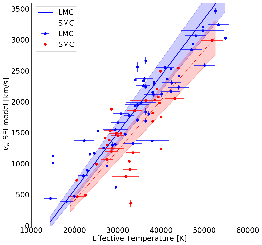
Figure 9: As Figure 6 but including $v_{\infty}$ measurements up to quality rank ii.

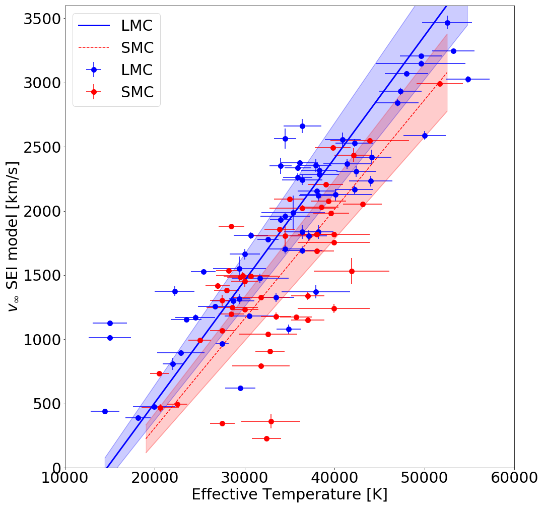
Figure 10: As Figure 6, but including $v_{\infty}$ measurements up to quality rank iii.

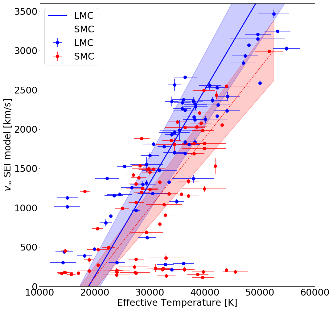
Figure 11: As Figure 6, but including $v_{\infty}$ measurements up to quality rank iv.

Here we present the same analysis as in Sect. 5.2, but now including measurements of poorer quality ranks. The inclusion of each consecutive decreasing rank is shown in Figs. 9 to 11. Including rank ii measurements increases the slopes in both environments, but both agree with rank i findings within the errors. This might indicate that including wind speed measurements from unsaturated profiles, which are lower than the true $v_{\infty}$ , has a systematic effect on the slope. This effect is exacerbated when adding rank iii measurements, which may be even farther from the true $v_{\infty}$. In a few cases, the $v_{\infty}$ lies far above the slope. The spectral types collected from the literature for these stars may not be correct. Updating spectral types for the ULLYSES sample is beyond the scope of this study. Rank iv measurements are for stars with little to no wind signatures, a large portion of which can be seen in Fig. 11 to have high temperatures. This is likely linked to the weak-wind problem where we are unable to diagnose $v_{\infty}$ from UV resonance lines. Therefore, there is little motivation to include these measurements when investigating $v_{\infty}$. In Sect. 5.2 we only used quality rank i measurements, that is, saturated line profiles.

Appendix C Trends by luminosity class

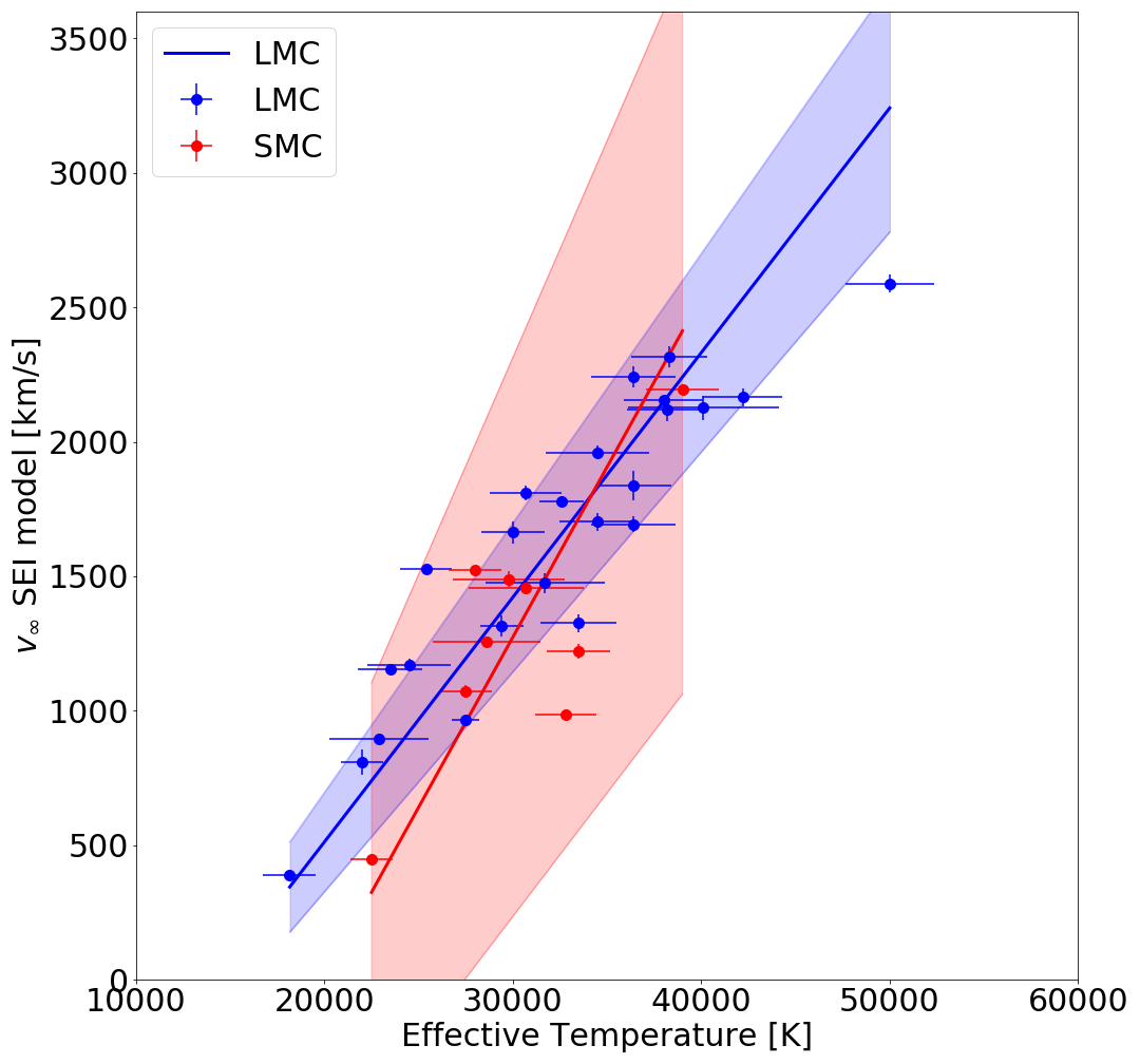
Figure 12: As Figure 6, but showing only $v_{\infty}$ measurements for supergiant stars.

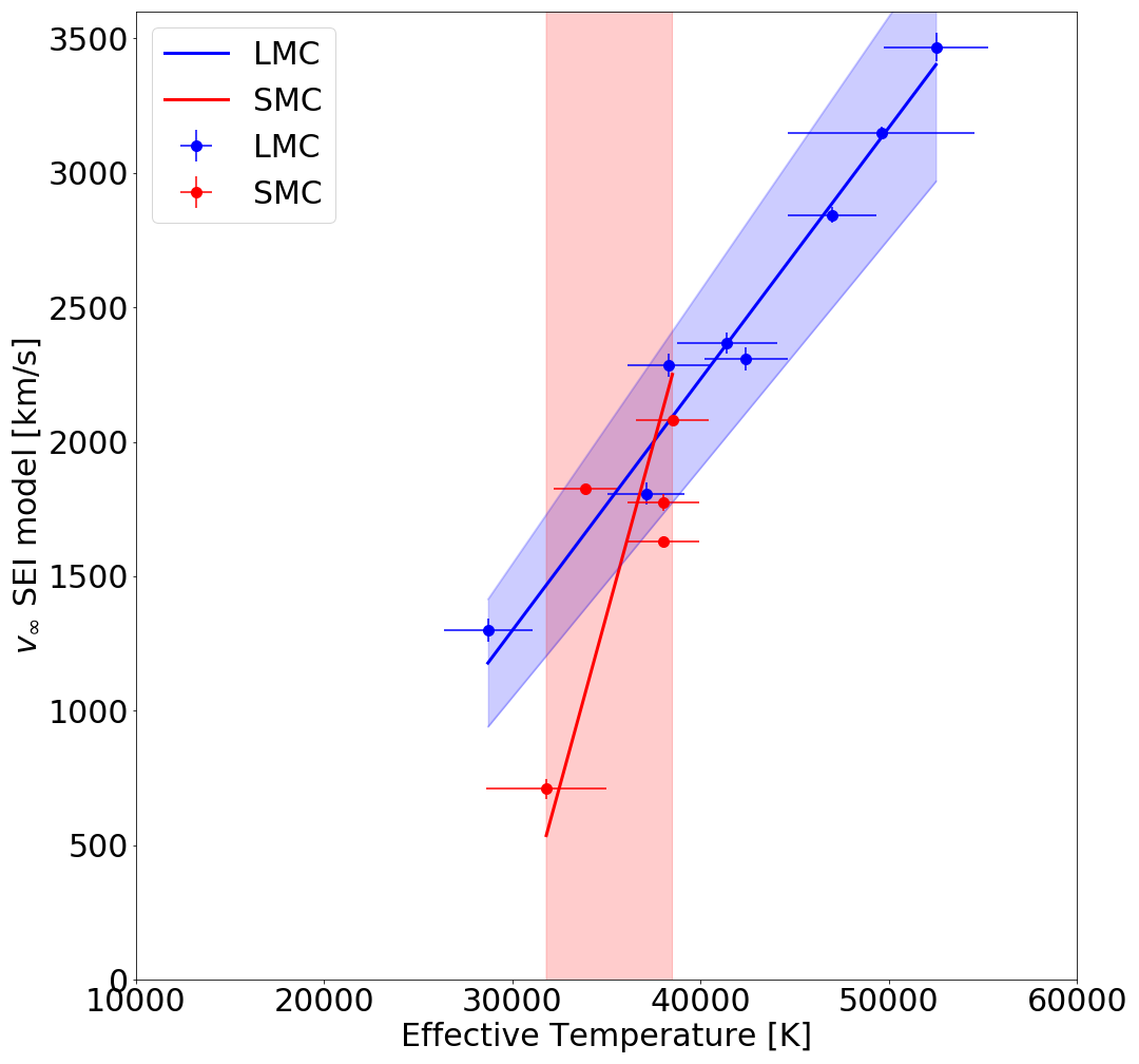
Figure 13: As Figure 6, but showing only $v_{\infty}$ measurements for giant stars.

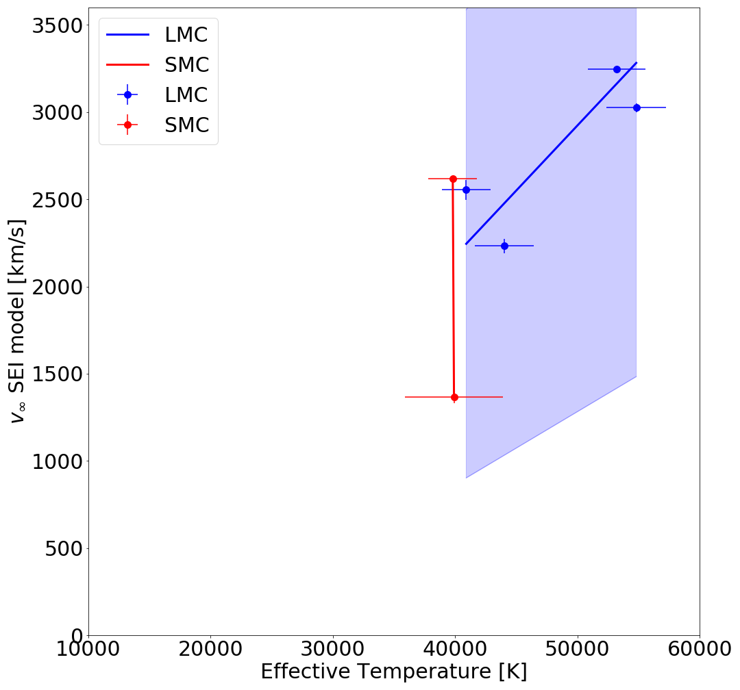
Figure 14: As Figure 6, but showing only $v_{\infty}$ measurements for dwarf stars.

Here we show the effect of analysing the sample split by luminosity class. The sub-samples for supergiants alone (luminosity class I) in the LMC and SMC are shown in Fig. 12. The sub-samples for giants and bright giants alone (luminosity class III) in the LMC and SMC are shown in Fig. 13. The sub-samples for dwarfs and sub-dwarfs alone (luminosity class V) in the LMC and SMC are shown in Fig. 14. For the LMC, the slopes are not affected sufficiently to motivate analysing the trends by luminosity class. The low number of high-quality measurements prevent this comparison in the SMC.

Appendix D Galactic samples

Table 8: ODR fit coefficients to relations between $v_{\infty}$ and $T_{\rm{eff}}$ as described in Eq. 3.

Region	a	b	RMS	Sample
	[$10^{-2}$]	[$\rm{km}\,\rm{s^{-1}}$]	[$\rm{km}\,\rm{s^{-1}}$]
LMC	$9.2\pm 0.6$	$1270\pm 200$	385	LMC-ii
SMC	$9.9\pm 1.1$	$1630\pm 350$	452	SMC-ii
LMC	$9.5\pm 0.7$	$1400\pm 230$	407	LMC-iii
SMC	$12.6\pm 1.8$	$2600\pm 560$	594	SMC-iii
LMC	$11.8\pm 1.1$	$2240\pm 380$	645	LMC-iv
SMC	$11.7\pm 1.6$	$2190\pm 420$	987	SMC-iv
LMC	$9.1\pm 0.9$	$1310\pm 280$	268	LMC-I
SMC	$12.6\pm 3.5$	$2520\pm 1010$	346	SMC-I
LMC	$9.3\pm 0.8$	$1500\pm 340$	118	LMC-III
SMC	$25.6\pm 21.6$	$7600\pm 7920$	443	SMC-III
LMC	$7.5\pm 3.3$	$810\pm 160$	238	LMC-V
SMC	n/a	n/a	n/a	SMC-V
GAL	$9.8\pm 0.3$	$1230\pm 960$	326	G
GAL	$10.2\pm 0.4$	$1340\pm 120$	291	H
GAL	$10.2\pm 0.3$	$1300\pm 100$	278	M

• The column ’sample’ indicates the metallicity environment and whether the slope is measured for a poorer quality rank (lower case roman numerals) or limited to a specific luminosity class (upper case roman numerals).

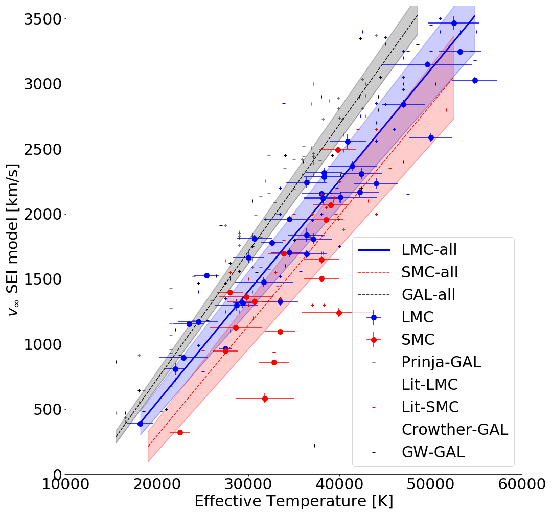
Figure 15: As Figure 8, but also including Galactic samples from Groenewegen et al. (1989) and Crowther et al. (2006).

We present the inclusion of the Groenewegen et al. (1989) and Crowther et al. (2006) samples in the Galactic relation. This is sample G in Table 8. The slope of the relation including these samples agrees slightly better with our findings in the LMC and SMC, but the quality of the $v_{\infty}$ measurements in these studies is difficult to verify.

As discussed in Sect. 5.3, we updated the stellar parameters of the Galactic O star sample with results obtained through quantitative spectroscopy. The work of Holgado et al. (2020) provides best-fit parameters from quantitative spectroscopy of optical spectra using FASTWIND models. The sample of Holgado et al. (2020) comprises more than 400 stars from the Galactic O star catalogue and includes 93% of the Prinja et al. (1990) sample with saturated C IV $\lambda\lambda$1548-1550 profiles. Only 72% of the stars have spectroscopic best-fit solutions, however, because 20 objects were identified as double-line spectroscopic binaries (SB2). For the purpose of updating the stellar parameters for this study, we used effective temperatures from Holgado et al. (2020) when available and excluded SB2 stars from the sample. This is presented as sample H in Table 8. As there is no UV component to the Holgado et al. (2020) study, we used the terminal wind speeds found Prinja et al. (1990). We also tested the effect of using the full Prinja et al. (1990) O star sample with saturated wind profiles. In this case, we used the full Prinja et al. (1990) sample by updating spectral types using the Galactic O Star Spectroscopic Survey (GOSSS; Sota et al. 2011, 2014; Maíz Apellániz et al. 2016) and used them to determine stellar parameters from the observational temperature calibrations of Martins et al. (2005). This is sample M in Table 8. The result of this is an overall slight upward revision of the terminal wind speed for a given effective temperature, as shown in Fig. 16, resulting in a slightly steeper metallicity dependence of $v_{\infty}\propto Z^{0.24\pm 0.03}$, which is not significantly different from the relation found using the effective temperatures from Holgado et al. (2020).

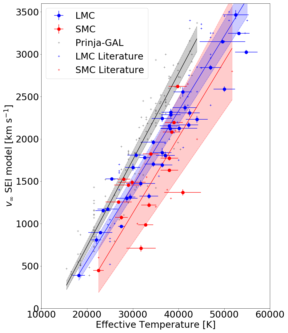
Figure 16: As Figure 8, but using the full Galatic O star sample with saturated wind profiles from Prinja et al. (1990).