Neural Pre-Processing: A Learning Framework for End-to-end Brain MRI Pre-processing

Abstract

Head MRI pre-processing involves converting raw images to an intensity-normalized, skull-stripped brain in a standard coordinate space. In this paper, we propose an end-to-end weakly supervised learning approach, called Neural Pre-processing (NPP), for solving all three sub-tasks simultaneously via a neural network, trained on a large dataset without individual sub-task supervision. Because the overall objective is highly under-constrained, we explicitly disentangle geometric-preserving intensity mapping (skull-stripping and intensity normalization) and spatial transformation (spatial normalization). Quantitative results show that our model outperforms state-of-the-art methods which tackle only a single sub-task. Our ablation experiments demonstrate the importance of the architecture design we chose for NPP. Furthermore, NPP affords the user the flexibility to control each of these tasks at inference time. The code and model are freely-available at https://github.com/Novestars/Neural-Pre-processing.

1 Introduction

Brain magnetic resonance imaging (MRI) is widely-used in clinical practice and neuroscience. Many popular toolkits for pre-processing brain MRI scans exist, e.g., FreeSurfer [9], FSL [25], AFNI [5], and ANTs [3]. These toolkits divide up the pre-processing pipeline into sub-tasks, such as skull-stripping, intensity normalization, and spatial normalization/registration, which often rely on computationally-intensive optimization algorithms.

Recent works have turned to machine learning-based methods to improve pre-processing efficiency. These methods, however, are designed to solve individual sub-tasks, such as SynthStrip [15] for skull-stripping and Voxelmorph [4] for registration. Learning-based methods have advantages in terms of inference time and performance. However, solving sub-tasks independently and serially has the drawback that each step’s performance depends on the previous step. In this paper, we propose a neural network-based approach, which we term Neural Pre-Processing (NPP), to solve three basic tasks of pre-processing simultaneously.

NPP first translates a head MRI scan into a skull-stripped and intensity-normalized brain using a translation module, and then spatially transforms to the standard coordinate space with a spatial transform module. As we demonstrate in our experiments, the design of the architecture is critical for solving these tasks together. Furthermore, NPP offers the flexibility to turn on/off different pre-processing steps at inference time. Our experiments demonstrate that NPP achieves state-of-the-art accuracy in all the sub-tasks we consider.

2 Methods

2.1 Model

As shown in Fig. 1, our model contains two modules: a geometry-preserving translation module, and a spatial-transform module.

2.1.1 Geometry-preserving Translation Module.

This module converts a brain MRI scan to a skull-stripped and intensity normalized brain. We implement it using a U-Net style [23] $f_{\theta}$ architecture (see Fig. 1), where $\theta$ denotes the model weights. We operationalize skull stripping and intensity normalization as a pixel-wise multiplication of the input image with a scalar multiplier field $\chi$, which is the output of the U-Net $f_{\theta}$:

$$T_{\theta}(x)=f_{\theta}(x)\otimes x,$$ (1)

where $\otimes$ denotes the element-wise (Hadamard) product.

Such a parameterization allows us to impose constraints on $\chi$. In this work, we penalize high-frequencies in $\chi$, via the total variation loss described below. Another advantage of $\chi$ is that it can be computed at a lower resolution to boost both training and inference speed, and then up-sampled to the full resolution grid before being multiplied with the input image. This is possible because the multiplier $\chi$ is spatially smooth. In contrast, if we have $f_{\theta}$ directly compute the output image, doing this at a lower resolution means we will inevitably lose high frequency information. In our experiments, we take advantage of this by having the model output the multiplicative field at a grid size that is 1/2 of the original input grid size along each dimension.

2.1.2 Spatial Transformation Module.

Spatial normalization is implemented as a variant of the Spatial Transformer Network (STN) [17]; in our implementation, the STN outputs the 12 parameters of an affine matrix $\Phi_{aff}$. The STN takes as input the bottleneck features from the image translation network $f_{\theta}$ and feeds it through a multi-layer perceptron (MLP) that projects the features to a 12-dimensional vector encoding the affine transformation matrix. This affine transformation is in turn applied to the output of the image translation module $T_{\theta}(x)$ via a differentiable resampling layer [17].

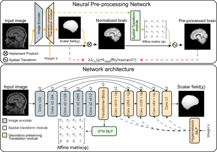
Figure 1: (Top) An overview of Neural Pre-processing. (Bottom) The network archiecture of Neural Pre-processing

2.2 Loss Function

The objective to minimize is composed of two terms. The first term is a reconstruction loss $L_{rec}$. In this paper, we use SSIM [29] for $L_{rec}$. The second term penalizes $T_{\theta}$ from making high-frequency intensity changes to the input image, encapsulating our prior knowledge that skull-stripping and MR bias field correction involve a pixel-wise product with a spatially smooth field. In this work, we use a total variation penalty [22] $L_{TV}$ on the multiplier field $\chi$, which promotes sparsity of spatial gradients in $\chi$. The final objective is:

$$\operatorname*{arg\,min}_{\theta}L_{rec}(T_{\theta}(x)\circ\Phi_{aff},x_{gt})+\lambda L_{TV}(\chi),$$ (2)

where $x_{gt}$ is the pre-processed ground truth images, $\lambda\geq 0$ controls the trade-off between the two loss terms, and $\circ$ denotes a spatial transformation.

2.2.1 Conditioning on $\lambda$.

Classically, hyperparameters like $\lambda$ are tuned on a held-out validation set - a computationally-intensive task which requires training multiple models corresponding to different values of $\lambda$. To avoid this, we condition on $\lambda$ in $f_{\theta}$ by passing in $\lambda$ as an input to a separate MLP $h_{\phi}(\lambda)$ (see Fig. 1), which generates a $\lambda$-conditional scale and bias for each channel of the decoder layers. $h_{\phi}$ can be interpreted as a hypernetwork [12, 28, 14] which generates a conditional scale and bias similar to adaptive instance normalization (AdaIN) [16].

Specifically, for a given decoder layer with $C$ intermediate feature maps $\{z_{1},...,z_{C}\}$, $h_{\phi}(\lambda)$ generates the parameters to scale and bias each channel $z_{c}$ such that the the channel values are computed as:

$$\hat{z}_{c}={\alpha_{c}z_{c}}+\beta_{c},$$ (3)

for $c\in\{1,...,C\}$. Here, $\alpha_{c}$ and $\beta_{c}$ denote the scale and bias of channel $c$, conditioned on $\lambda$. This is repeated for every decoder layer, except the final layer.

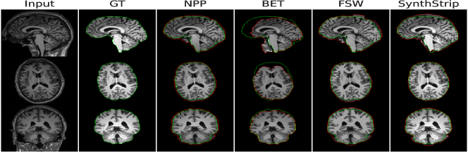
Figure 2: Representative slices for skull-stripping. From top to bottom: coronal, axial and sagittal views. Green and red contours depict ground truth and estimated brain masks, respectively.

3 Experiments

3.0.1 Training details.

We created a large-scale dataset of 3D T1-weighted (T1w) brain MRI volumes by aggregating 7 datasets: GSP [13], ADNI [21], OASIS [20], ADHD [24], ABIDE [30], MCIC [11], and COBRE [1]. The whole training set contains 10,083 scans. As ground-truth target images, we used FreeSurfer generated skull-stripped, intensity-normalized and affine-registered (to so-called MNI atlas coordinates) images.

We train NPP with ADAM [19] and a batch size of 2, for a maximum of 60 epochs. The initial learning rate is 1e-4 and then decreases by half after 30 epochs. We use random gamma transformation as a data augmentation technique, with parameter log gamma (-0.3,0.3). We randomly sampled $\lambda$ from a log-uniform distribution on $(-3,1)$ for each mini-batch.

3.0.2 Architecture Details.

$f_{\theta}$ is a U-Net-style architecture containing an encoder and decoder with skip connections in between. The encoder and decoder have 5 levels and each level consists of 2 consecutive 3D convolutional layers. Specifically, each 3D convolutional layer is followed by an instance normalization layer and LeakyReLU (negative slope of 0.01). In the bottleneck, we use three transformer blocks to enhance the ability of capturing global information [27]. Each transformer block contains a self-attention layer and a MLP layer. For the transformer block, we use patch size 1x1x1, 8 attention heads, and an MLP expansion ratio of 1. We perform tokenization by flattening the 3D CNN feature maps into a 1D sequence.

The hypernetwork, $h_{\phi}$, is a 3-layer MLP with hidden layers 512, 2048 and 496. The STN MLP is composed of a global average pooling layer and a 2-layer MLP with hidden layers of size 256 and 12. The 2-layer MLP contains: linear(256 channels); ReLU; linear(12 channels); Tanh. Note an identity matrix is added to the output affine matrix.

Method	SS	IN	SN	GPU	CPU
SynthStrip	16.5	-	-
BET	9.1	262.2	-
Freesurfer	747.2	481.5	671.6
NPP (Ours)	2.94

Table 1: Supported sub-tasks and average runtime for each method. Skull-stripping (SS), intensity normalization (IN) and spatial normalization (SN). Units are sec, bold is best.

Method	Rec SSIM	Rec PSNR	Bias SSIM	Bias PSNR
FSL	98.5	34.2	92.5	39.2
FS	98.9	35.7	92.1	39.3
NPP	99.1	36.2	92.7	39.4

Table 2: Performance on intensity normalization. Higher is better, bold is best.

3.0.3 Baselines.

We chose three popular and widely-used tools, SynthStrip [15], FSL [25], and FreeSurfer [9], as baselines. SynthStrip (SS) is a learning-based skull-stripping method, while FSL and FreeSurfer (FS) is a cross-platform brain processing package containing multiple tools. FSL’s Brain Extraction Tool (BET) and FMRIB’s Automated Segmentation Tool are for skull stripping and MR bias field correction, respectively. FS uses a watershed method for skull-stripping, a model-based tissue segmentation for intensity normalization and bias field correction.

3.1 Runtime analyses

The primary advantage of NPP is runtime. As shown in Table 2, for images with resolution $256\times 256\times 256$, NPP requires less than 3 sec on a GPU and less than 8 sec on a CPU for all three pre-processing tasks. This is in part due to the fact that the multiplier field can be computed at a lower resolution (in our case, on a grid of $128\times 128\times 128$). The output field is then up-sampled with trilinear interpolation before being multiplied with the input image. In contrast, SynthStrip needs 16.5 sec on a GPU for skull stripping. FSL’s optimized implementation takes about 271.3 sec per image for skull stripping and intensity normalization, whereas FreeSurfer needs more than 10 min.

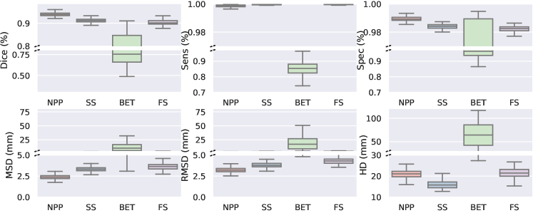
Figure 3: Skull-stripping performance on various metrics. (Top) Higher is better. (Bottom) Lower is better.

3.2 Pre-processing Performance

We empirically validate the performance of NPP for the three tasks we consider: skull-stripping, intensity normalization, and spatial transformation.

3.2.1 Evaluation Datasets.

For skull-stripping, we evaluate on the Neuralfeedback skull-stripped repository (NFSR) [7] dataset. NFSR contains 125 manually skull-stripped T1w images from individuals aged 21 to 45, and are diagnosed with a wide range of psychiatric diseases. The definition of the brain mask used in NFSR follows that of FS. For intensity normalization, we evaluate on the test set (N=856) from the Human Connectome Project (HCP). The HCP dataset includes T1w and T2w brain MRI scans which can be combined to obtain a high quality estimate of the bias field [26, 10]. For spatial normalization, we use T1w MRI scans from the Parkinson’s Progression Markers Initiative (PPMI). These images were automatically segmented using Freesurfer into anatomical regions of interest (ROIs) [6].

3.2.2 Metrics.

For skull-stripping, we quantify performance using the Dice overlap coefficient (Dice), Sensitivity (Sens), Specificity (Spec), mean surface distance (MSD), residual mean surface distance (RMSD), and Hausdorff distance (HD), as defined elsewhere [18]. For intensity normalization, we evaluate the intensity-normalized reconstruction (Rec) and estimated bias image (Bias, which is equal to the multiplier field $\chi$) to the ground truth images, using PSNR and SSIM. For spatial normalization, we quantify performance by the Dice score between the spatially transformed segmentations (resampled using the estimated affine transformation) and the probabilistic labels of the target atlas.

3.2.3 Results.

Fig 2 and Fig 3 shows skull-stripping performance for all models. We observe that the proposed method outperforms all traditional and learning-based baselines on Dice, Spec, and MSD/RMSD. Importantly, NPP achieved 93.8% accuracy and 2.7% improvement on Dice and 2.39mm MSD. Especially for MSD, NPP is 28% better than the second-best method, SynthStrip. We further observe that BET commonly fails, which has also been noted in the literature [8].

Table 2 shows the quantitative results of FSL, FS and NPP(see visualization results in Supplementary S1). NPP outperforms the baselines on all metrics. From Table 2, we see that FreeSurfer’s reconstruction is better than BET’s, but the bias field estimates are relatively worse. We can appreciate this in the figure in Supplementary S1, as we observe that FS’s bias field estimate (f) contains too much high-frequency anatomical detail.

Fig. 4 (b) shows boxplots of Dice scores for NPP and FreeSurfer, for each ROI. Compared to FS, NPP achieves consistent improvement on all ROIs measured. Fig. 4 (a) shows representative slices for spatial normalization.

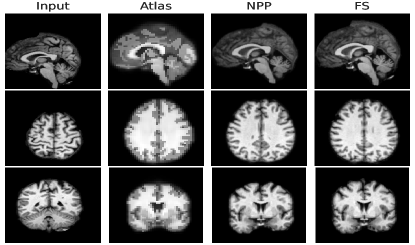
(a)

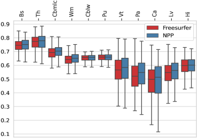
(b)

Figure 4: (a) Representative examples for spatial normalization. Rows depict sagittal, axial and coronal view. For each view, from left to right: input image, atlas, NPP results, and FreeSurfer results. (b) Boxplots illustrating Dice scores of each anatomical structure for NPP and FreeSurfer in the atlas-based registration with the PPMI dataset. We combine left and right hemispheres of the brain into one structure for visualization.

Table 3: Ablation study results of different $\lambda$. Bold is best.

Method	RecSSIM	Bias SSIM
NPP, $\lambda=10$	96.38 $\pm$ 1.29	96.02 $\pm$ 1.29
NPP, $\lambda=1$	99.07 $\pm$ 0.61	98.09 $\pm$ 0.62
NPP, $\lambda=0.1$	99.25 $\pm$ 0.52	98.40 $\pm$ 0.40
NPP, $\lambda=0.01$	99.24 $\pm$ 0.51	98.22 $\pm$0.39
NPP, $\lambda=0.001$	99.22 $\pm$ 0.52	98.13 $\pm$ 0.40

Table 4: Comparison with ablated models. Bold is best.

Method	Rec SSIM
Naive U-Net	84.12 $\pm$ 3.34
U-Net+STN	84.87$\pm$ 3.04
UMIRGPIT	84.26 $\pm$ 3.02
NPP, $\lambda=0.1$	99.25 $\pm$ 0.52

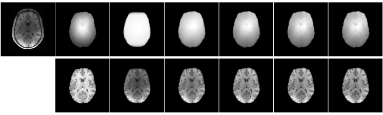
Figure 5: (Top) From left to right, raw input image, ground truth bias field, estimated multiplier fields from NPP for different values of $\lambda={10,1,0.1,0.01,0.001}$. (Bottom) From left to right, ground truth, outputs from NPP for different values of $\lambda$.

3.3 Ablation

As ablations, we compare the specialized architecture of NPP against a naive U-Net trained to solve all three tasks at once. Additionally, we implemented a different version of our model where the U-Net directly outputs the skull-stripped and intensity-normalized image, which is in turn re-sampled with the STN. In this version, we did not have the scalar multiplication field and thus our loss function did not include the total variation term. We call this version U-Net+STN. As another alternative, we trained the U-Net+STN architecture via UMIRGPIT [2], which encourages the translation network (U-Net) to be geometry-preserving by alternating the order of the translation and registration. We note again that for all these baselines, we used the same architecture as $f_{\theta}$, but instead of computing the multiplier field $\chi$, $f_{\theta}$ computes the final intensity-normalized and spatially transformed image directly. The objective is the reconstruction loss $L_{rec}$. All other implementation details were the same as NPP. For evaluation, we use the test images from the HCP dataset.

Results: Tables 4 and 4 lists the SSIM values for the estimated reconstruction and bias fields, for different ablations and NPP with a range of $\lambda$ values. We observe that there is a sweet spot around $\lambda=0.1$, which underscores the importance of considering different hyperparameter settings and affording the user to optimize this at test time. All ablation results are poor, supporting the importance of our architectural design. Fig. 5 shows some representative results for a range of $\lambda$ values.

4 Conclusion

In this paper, we propose a novel neural network approach for brain MRI pre-processing. The proposed model, called NPP, disentangles geometry-preserving translation mapping (which includes skull stripping and bias field correction) and spatial transformation. Our experiments demonstrate that NPP can achieve state-of-the-art results for the major tasks of brain MRI pre-processing.

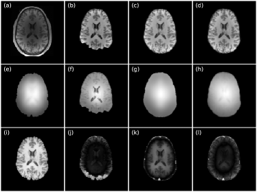
Figure 6: Representative slices of intensity normalization performance on HCP T1w brain images. (a) input image; (b-d) intensity normalized outputs from FreeSurfer, FSL, and NPP with $\lambda=0.1$; (e) ground truth bias field; (f-h) bias fields estimated by the corresponding methods; (i) ground-truth intensity normalized image; (j-l) prediction error maps corresponding to (b-d).

References

- [1] Aine, C.J., Bockholt, H.J., Bustillo, J.R., Cañive, J.M., Caprihan, A., Gasparovic, C., Hanlon, F.M., Houck, J.M., Jung, R.E., Lauriello, J., Liu, J., Mayer, A.R., Perrone-Bizzozero, N.I., Posse, S., Stephen, J.M., Turner, J.A., Clark, V.P., Calhoun, V.D.: Multimodal neuroimaging in schizophrenia: Description and dissemination. Neuroinformatics 15, 343–364 (10 2017)
- [2] Arar, M., Ginger, Y., Danon, D., Bermano, A.H., Cohen-Or, D.: Unsupervised multi-modal image registration via geometry preserving image-to-image translation. In: Proceedings of the IEEE/CVF conference on computer vision and pattern recognition. pp. 13410–13419 (2020)
- [3] Avants, B.B., Epstein, C.L., Grossman, M., Gee, J.C.: Symmetric diffeomorphic image registration with cross-correlation: Evaluating automated labeling of elderly and neurodegenerative brain. Medical Image Analysis 12, 26–41 (2 2008)
- [4] Balakrishnan, G., Zhao, A., Sabuncu, M.R., Guttag, J., Dalca, A.V.: Voxelmorph: A learning framework for deformable medical image registration. IEEE Transactions on Medical Imaging 38, 1788–1800 (8 2019)
- [5] Cox, R.W.: Afni: software for analysis and visualization of functional magnetic resonance neuroimages. Computers and Biomedical research 29(3), 162–173 (1996)
- [6] Dalca, A.V., Guttag, J., Sabuncu, M.R.: Anatomical priors in convolutional networks for unsupervised biomedical segmentation. In: Proceedings of the IEEE Conference on Computer Vision and Pattern Recognition. pp. 9290–9299 (2018)
- [7] Eskildsen, S.F., Coupé, P., Fonov, V., Manjón, J.V., Leung, K.K., Guizard, N., Wassef, S.N., Østergaard, L.R., Collins, D.L.: Beast: Brain extraction based on nonlocal segmentation technique. NeuroImage 59, 2362–2373 (2 2012)
- [8] Ezhilarasan, K., Praveenkumar, S., Somasundaram, K., Kalaiselvi, T., Magesh, S., Kiruthika, S., Jeevarekha, A.: Automatic brain extraction from mri of human head scans using helmholtz free energy principle and morphological operations. Biomedical Signal Processing and Control 64, 102270 (2021)
- [9] Fischl, B.: Freesurfer. Neuroimage 62(2), 774–781 (2012)
- [10] Glasser, M.F., Sotiropoulos, S.N., Wilson, J.A., Coalson, T.S., Fischl, B., Andersson, J.L., Xu, J., Jbabdi, S., Webster, M., Polimeni, J.R., Essen, D.C.V., Jenkinson, M.: The minimal preprocessing pipelines for the human connectome project. NeuroImage 80, 105–124 (10 2013)
- [11] Gollub, R.L., Shoemaker, J.M., King, M.D., White, T., Ehrlich, S., Sponheim, S.R., Clark, V.P., Turner, J.A., Mueller, B.A., Magnotta, V., O’Leary, D., Ho, B.C., Brauns, S., Manoach, D.S., Seidman, L., Bustillo, J.R., Lauriello, J., Bockholt, J., Lim, K.O., Rosen, B.R., Schulz, S.C., Calhoun, V.D., Andreasen, N.C.: The mcic collection: A shared repository of multi-modal, multi-site brain image data from a clinical investigation of schizophrenia. Neuroinformatics 11, 367–388 (7 2013)
- [12] Ha, D., Dai, A., Le, Q.V.: Hypernetworks (9 2016), http://arxiv.org/abs/1609.09106
- [13] Holmes, A.J., Hollinshead, M.O., O’Keefe, T.M., Petrov, V.I., Fariello, G.R., Wald, L.L., Fischl, B., Rosen, B.R., Mair, R.W., Roffman, J.L., Smoller, J.W., Buckner, R.L.: Brain genomics superstruct project initial data release with structural, functional, and behavioral measures. Scientific Data 2 (7 2015)
- [14] Hoopes, A., Hoffmann, M., Fischl, B., Guttag, J., Dalca, A.V.: Hypermorph: Amortized hyperparameter learning for image registration (1 2021), http://arxiv.org/abs/2101.01035
- [15] Hoopes, A., Mora, J.S., Dalca, A.V., Fischl, B., Hoffmann, M.: Synthstrip: skull-stripping for any brain image. NeuroImage 260, 119474 (2022)
- [16] Huang, X., Belongie, S.: Arbitrary style transfer in real-time with adaptive instance normalization. In: Proceedings of the IEEE international conference on computer vision. pp. 1501–1510 (2017)
- [17] Jaderberg, M., Simonyan, K., Zisserman, A., et al.: Spatial transformer networks. Advances in neural information processing systems 28 (2015)
- [18] Jadon, S.: A survey of loss functions for semantic segmentation. In: 2020 IEEE Conference on Computational Intelligence in Bioinformatics and Computational Biology (CIBCB). pp. 1–7. IEEE (2020)
- [19] Kingma, D.P., Ba, J.: Adam: A method for stochastic optimization (12 2014), http://arxiv.org/abs/1412.6980
- [20] Marcus, D.S., Fotenos, A.F., Csernansky, J.G., Morris, J.C., Buckner, R.L.: Open access series of imaging studies: longitudinal mri data in nondemented and demented older adults. Journal of cognitive neuroscience 22(12), 2677–2684 (2010)
- [21] Mueller, S.G., Weiner, M.W., Thal, L.J., Petersen, R.C., Jack, C., Jagust, W., Trojanowski, J.Q., Toga, A.W., Beckett, L.: The alzheimer’s disease neuroimaging initiative. Neuroimaging Clinics 15(4), 869–877 (2005)
- [22] Osher, S., Burger, M., Goldfarb, D., Xu, J., Yin, W.: An iterative regularization method for total variation-based image restoration. Multiscale Modeling and Simulation 4, 460–489 (2005)
- [23] Ronneberger, O., Fischer, P., Brox, T.: U-net: Convolutional networks for biomedical image segmentation. In: Medical Image Computing and Computer-Assisted Intervention–MICCAI 2015: 18th International Conference, Munich, Germany, October 5-9, 2015, Proceedings, Part III 18. pp. 234–241. Springer (2015)
- [24] Sibley, M.H., Coxe, S.J.: The adhd teen integrative data analysis longitudinal (tidal) dataset: Background, methodology, and aims. BMC Psychiatry 20 (7 2020)
- [25] Smith, S.M., Jenkinson, M., Woolrich, M.W., Beckmann, C.F., Behrens, T.E., Johansen-Berg, H., Bannister, P.R., Luca, M.D., Drobnjak, I., Flitney, D.E., Niazy, R.K., Saunders, J., Vickers, J., Zhang, Y., Stefano, N.D., Brady, J.M., Matthews, P.M.: Advances in functional and structural mr image analysis and implementation as fsl. vol. 23 (2004)
- [26] Song, W., Zeng, C., Zhang, X., Wang, Z., Huang, Y., Lin, J., Wei, W., Qu, X.: Jointly estimating bias field and reconstructing uniform mri image by deep learning. Journal of Magnetic Resonance 343 (10 2022)
- [27] Vaswani, A., Shazeer, N., Parmar, N., Uszkoreit, J., Jones, L., Gomez, A.N., Kaiser, Ł., Polosukhin, I.: Attention is all you need. Advances in neural information processing systems 30 (2017)
- [28] Wang, A.Q., Dalca, A.V., Sabuncu, M.R.: Computing multiple image reconstructions with a single hypernetwork. Machine Learning for Biomedical Imaging 1 (2022)
- [29] Wang, Z., Bovik, A.C., Sheikh, H.R., Simoncelli, E.P.: Image quality assessment: From error visibility to structural similarity. IEEE Transactions on Image Processing 13, 600–612 (4 2004)
- [30] de Wilde, A., van Maurik, I.S., Kunneman, M., Bouwman, F., Zwan, M., Willemse, E.A., Biessels, G.J., Minkman, M., Pel, R., Schoonenboom, N.S., et al.: Alzheimer’s biomarkers in daily practice (abide) project: rationale and design. Alzheimer’s & Dementia: Diagnosis, Assessment & Disease Monitoring 6, 143–151 (2017)