Robust Exponential Runge–Kutta Embedded Pairs

Abstract

Exponential integrators are explicit methods for solving ordinary differential equations that treat linear behaviour exactly. The stiff-order conditions for exponential integrators derived in a Banach space framework by Hochbruck and Ostermann are solved symbolically by expressing the Runge–Kutta weights as unknown linear combinations of phi functions. Of particular interest are embedded exponential pairs that efficiently generate both a high- and low-order estimate, allowing for dynamic adjustment of the time step. A key requirement is that the pair be robust: if the nonlinear source function has nonzero total time derivatives, the order of the low-order estimate should never exceed its design value. Robust exponential Runge–Kutta (3,2) and (4,3) embedded pairs that are well-suited to initial value problems with a dominant linearity are constructed.

65L04, 65L06, 65M22

1 Introduction

Nonlinear initial value problems arise frequently in science and engineering applications. In contrast with linear first-order ordinary differential equations, which may be readily solved with the introduction of an appropriate integrating factor, the solution of nonlinear initial-value problems typically requires numerical approximation.

Many dynamical equations contain both linear and nonlinear effects. In the limit when the linear time scale becomes much shorter than the nonlinear time scale, it is desirable to solve for the evolution exactly, for both accuracy and numerical stability. For such problems, it may at first seem sufficient to simply incorporate the linearity into an integrating factor; in the absence of the nonlinearity, the resulting algorithm would then be exact. However, such integrating factor methods do not solve nonlinear problems accurately, even on the linear time scale, since the implicit treatment of the linear term introduces an integrating factor (which varies on the linear time scale) into the explicitly computed nonlinearity. Fortunately there exist better methods, known as exponential integrators, that are well-suited to such problems: exponential integrators of order $p$ are exact whenever the nonlinear term is a polynomial in time of degree less than $p$.

Consider an initial value problem of the form

(1) $$\frac{dy}{dt}=f(t,y(t))=F(t,y(t))-Ly,\qquad y(0)=y_{0},$$

where $y$ is a vector, $F$ is an analytic function, and $L$ is a constant matrix, with initial condition $y_{0}$. One can compute a numerical approximation of a future estimate $y_{n+1}$ for $n\geq 0$ using an explicit $s$-stage Runge–Kutta (RK) method:

(2) $$y_{n}^{i+1}=y_{n}^{0}+h\sum_{j=0}^{i}a_{ij}f(t_{n}+c_{j}h,y_{n}^{j})\quad i=0,\dots,s-1,$$

where $y_{0}^{0}=y_{0}$, $y_{n+1}=y_{n}^{s}$, $h$ is the time step, $t_{n}=nh$, the scalar constants $a_{ij}$ are the Runge–Kutta weights, and $c_{j}$ are the step fractions for stage $j$. For $n\geq 1$, $y_{n}^{0}=y_{n-1}^{s}$ is the approximation of the solution at time $nh$, also denoted by $y_{n}$. The weights can be organized into a Butcher tableau (Table 1).

$$\begin{array}[]{c|cccccc}0\\ c_{1}&a_{00}\\ c_{2}&a_{10}&a_{11}\\ \vdots&\vdots&\vdots&\ddots\\ c_{s-1}&a_{(s-2)0}&\cdots&\cdots&a_{(s-2)(s-2)}\\ \hline\cr 1&a_{(s-1)0}&\cdots&\cdots&a_{(s-1)(s-1)}\\ \end{array}$$

Table 1: General Runge–Kutta tableau.

For problems where the linear time scale is much shorter than the nonlinear time scale, explicit Runge–Kutta methods require a very small time step to maintain stability and accuracy. This behaviour is often called numerical stiffness and is defined precisely in [23] and references therein. Exponential Runge–Kutta (ERK) integrators are explicit methods that are designed for linearly stiff differential equations. They have a similar structure to explicit Runge–Kutta methods, except that the weights $a_{ij}$ are now matrix functions of $L$:

(3) $$y_{n}^{i+1}=e^{-hL}y_{n}^{0}+h\sum_{j=0}^{i}a_{ij}(-hL)F(t_{n}+c_{j}h,y_{n}^{j})\quad i=0,\dots,s-1.$$

We describe these methods in Section 2 and introduce in Section 3 computationally viable embedded exponential pairs that can be used for adaptive time stepping of practical problems in science and engineering.

We conclude the paper with some numerical examples and applications in Section 4.

2 Exponential Integrators

In the scalar case, the global error of the explicit Euler method grows uncontrollably when $F(t,y)=0$ and $L\tau>2$. The failure of explicit methods when $L$ is large is often ascribed in the literature to numerical stiffness [15]. First introduced by Certaine in 1960 [6], exponential integrators avoid stiffness arising from the linear term by treating it exactly.

By defining $G(t)=F(t,y(t))$, the integrating factor $I(t)=e^{tL}$, and $Y(t)=I(t)y(t)$, we can transform (1) to

(4) $$\frac{dY}{dt}=I(t)G(t),\quad Y(0)=y_{0}.$$

Discretizing in the $t$ variable directly leads to integrating factor methods. However, the change of variable $I\,dt=L^{-1}\,dI$ transforms (4) to

(5) $$\frac{dY}{dI}=L^{-1}G(L^{-1}\log(I)).$$

Letting $t=t_{n}+\tau$, we can Taylor expand $G(t_{n}+\tau)$ about $t_{n}$:

(6) $$G(t_{n}+\tau)=\sum_{k=0}^{\infty}\frac{\tau^{k}}{k!}G^{(k)}(t_{n}),$$

so that (5) becomes

(7) $$\frac{dY}{dI}=L^{-1}\sum_{k=0}^{\infty}\frac{{\left(L^{-1}\log(Ie^{-t_{n}L})\right)}^{k}}{k!}G^{(k)}(t_{n}).$$

On integrating from $I(t_{n})$ to $I(t_{n}+h)$, we obtain

(8) $$Y(t_{n}+h)=Y(t_{n})+L^{-1}\sum_{k=0}^{\infty}G^{(k)}(t_{n})\frac{1}{k!}\int_{I(t_{n})}^{I(t_{n}+h)}{\left(L^{-1}\log(\tilde{I}e^{-t_{n}L})\right)}^{k}\,d\tilde{I}.$$

We can change the integration variable from $\tilde{I}$ to $\bar{I}=I(-t_{n})\tilde{I}$ to obtain

(9) $$Y(t_{n}+h)=Y(t_{n})+L^{-1}\sum_{k=0}^{\infty}G^{(k)}(t_{n})\frac{1}{k!}\int_{1}^{I(h)}{\left(L^{-1}\log\bar{I}\right)}^{k}I(t_{n})\,d\bar{I}$$

and then transform back to the original variables, noting $\bar{I}=e^{\tau L}$:

(10) $$e^{(t_{n}+h)L}y(t_{n}+h)=e^{t_{n}L}y(t_{n})+L^{-1}\sum_{k=0}^{\infty}G^{(k)}(t_{n})\frac{1}{k!}\int_{0}^{h}\tau^{k}e^{t_{n}L}Le^{\tau L}\,d\tau.$$

This result simplifies to

(11) $$y(t_{n}+h)=e^{-hL}y(t_{n})+e^{-hL}\sum_{k=0}^{\infty}G^{(k)}(t_{n})\int_{0}^{h}\frac{\tau^{k}}{k!}e^{\tau L}\,d\tau.$$

We can make this representation of the solution more compact by defining $\varphi_{0}(x)=e^{x}$ and

(12) $$\varphi_{k}(-hL)=\frac{1}{h^{k}}\int_{0}^{h}\frac{\tau^{k-1}}{(k-1)!}e^{-(h-\tau)L}\,d\tau\text{ for }k\in{\mathbb{N}}.$$

Integrating (12) by parts leads to an inductive relation for the $\varphi_{k}$ functions:

(13) $$\varphi_{k}(0) =\frac{1}{k!},$$

(14) $$\varphi_{0}(x) =e^{x},$$

(15) $$\varphi_{k+1}(x) =\frac{\varphi_{k}(x)-\frac{1}{k!}}{x}\text{ for }k\geq 0.$$

The exact solution to (1) then becomes

(16) $$y(t_{n}+h)=e^{-hL}y(t_{n})+\sum_{k=0}^{\infty}h^{k+1}\varphi_{k+1}G^{(k)}(t_{n}),$$

which agrees with equation (4.6) of Ref. [12], which Hochbruck and Ostermann then use to derive order conditions for stiff differential equations. In the literature, (16) is typically obtained with the variation-of-constants method:

(17) $$y(t_{n}+h)=e^{-hL}y(t_{n})+e^{-hL}\int_{0}^{h}e^{\tau L}F(t_{n}+\tau,y(t_{n}+\tau))\,d\tau.$$

Since this is the exact solution of (1), the task of coming up with an exponential Runge–Kutta method becomes equivalent to approximating the infinite sum in (16) or the integral in (17). The simplest approximation of the integral in (17) takes $F$ to be constant:

$$y(t_{n}+h) =e^{-hL}y(t_{n})+e^{-hL}\int_{0}^{h}e^{\tau L}F(t_{n},y(t_{n}))\,d\tau$$

$$=e^{-hL}y_{n}+\frac{e^{-hL}-1}{-L}F(t_{n},y_{n})$$

$$=\varphi_{0}(-hL)y_{n}+h\varphi_{1}(-hL)F(t_{n},y_{n}).$$

The above approximation is called the exponential Euler method; it reduces to the explicit Euler method in the classical limit $L\to 0$.

The exponential Euler method solves (1) exactly whenever $F(t,y)$ is constant. In contrast, the integrating factor Euler method (IF Euler),

(18) $$y(t_{n}+h)=e^{-hL}(y_{n}+hF(t_{n},y_{n})),$$

which has been widely applied to stiff problems, is exact only when $F(t,y)=0$ and does not preserve fixed points of the original ordinary differential equation [14, 7, 3], as shown in Figure 2, where we compare various Euler methods (explicit, implicit, integrator factor, and exponential), for $F(t,y)=1/y$, with $y_{0}=1$. The orders of these methods at $t=1$ are demonstrated in Figure 2.

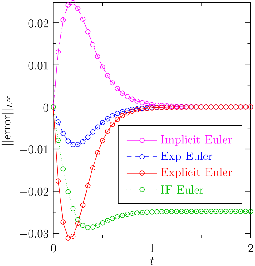
Figure 1: Evolution of the error for $dy/dt=1/y-Ly$ using the explicit, implicit, integrating factor, and exponential Euler methods with $h=0.05$.

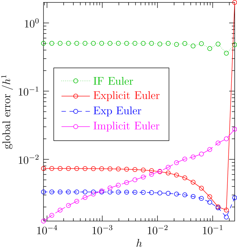
Figure 2: Error vs. timestep for $dy/dt=1/y-Ly$ using the explicit, implicit, integrating factor, and exponential Euler methods at $t=1$.

Just like in the classical case, there exist high-order exponential integrator methods. Cox and Matthews [7] attempted to approximate the integral in (17) with polynomials of degree higher than one and subsequently claimed to have derived a fourth-order scheme that they called ETD4RK. For the sake of bringing consistency to the names of methods by different authors, we denote it ERK4CM and give its Butcher tableau in Table 2.

$$\begin{array}[]{c|cccc}0\\ \frac{1}{2}&\frac{1}{2}\varphi_{1}{\left(-\frac{hL}{2}\right)}\\ \frac{3}{4}&0&\frac{1}{2}\varphi_{1}{\left(-\frac{hL}{2}\right)}\\ 1&\frac{1}{2}\varphi_{1}{\left(-\frac{hL}{2}\right)}\Bigl{(}\varphi_{0}{\left(-\frac{hL}{2}\right)}-1\Bigr{)}&0&\varphi_{1}{\left(-\frac{hL}{2}\right)}\\ \hline\cr 1&\varphi_{1}-3\varphi_{2}+4\varphi_{3}&2\varphi_{2}-4\varphi_{3}&2\varphi_{2}-4\varphi_{3}&4\varphi_{3}-\varphi_{2}\end{array}$$

Table 2: ERK4CM tableau, where $\varphi_{i}=\varphi_{i}(-hL)$.

Krogstad [14] takes a different route than Cox and Matthews. Instead of approximating the integral in (17), he truncates the series in (16) in a way that allows for control of the remainder. He discovered an improved version of ERK4CM that he claims is fourth order and denotes by ETDRK4-B. We denote Krogstad’s method by ERK4K and give its Butcher tableau in Table 3.

$$\begin{array}[]{c|cccc}0\\ \frac{1}{2}&\frac{1}{2}\varphi_{1}{\left(-\frac{hL}{2}\right)}\\ \frac{1}{2}&\frac{1}{2}\varphi_{1}{\left(-\frac{hL}{2}\right)}-\varphi_{2}{\left(-\frac{hL}{2}\right)}&\varphi_{2}{\left(-\frac{hL}{2}\right)}\\ 1&\varphi_{1}-2\varphi_{2}&0&2\varphi_{2}\\ \hline\cr 1&\varphi_{1}-3\varphi_{2}+4\varphi_{3}&2\varphi_{2}-4\varphi_{3}&2\varphi_{2}-4\varphi_{3}&4\varphi_{3}-\varphi_{2}\end{array}$$

Table 3: ERK4K tableau, where $\varphi_{i}=\varphi_{i}(-hL)$.

Not long after Krogstad introduced ERK4K, Hochbruck and Ostermann [12] published a rigorous framework for deriving exponential integrators. They argued that simply trying to approximate the integral in (17) was not enough to guarantee that the methods would retain their order for all stiff problems. As counterexamples, they presented a problem (Fig. 4) for which ERK4CM exhibits order two (instead of the claimed order four) and ERK4K exhibits order three (instead of the claimed order four). It became apparent that there is a concrete distinction between the order conditions for classical and exponential Runge–Kutta methods. In their Theorem 4.7, Hochbruck and Ostermann derive stiff-order conditions (Table 4) up to order four that describe sufficient conditions for an exponential RK method to not suffer a stiff-order reduction.

The operators $J$ and $K$ appearing in the order conditions in Table 4 are discretizations of the bounded operators

(19) $$J_{n}=\frac{\partial F}{\partial y}(t_{n},y(t_{n})),\quad K_{n}=\frac{\partial^{2}F}{\partial t\partial y}(t_{n},y(t_{n})).$$

In the case of a single stiff ordinary differential equation, $J$ and $K$, as well as the weights of the method, are scalars, so that $J$ and $K$ cancel from the stiff-order equations. If we want a method to retain its order even when solving arbitrary systems of stiff equations, we need to be more careful. In this case, the operators $J$ and $K$ are matrices. Moreover, the weights $a_{ij}$ of the method are simply linear combinations of $\varphi_{k}$ functions evaluated at scalar multiples of the matrix $L$. Therefore, the operators $J$ and $K$ do not necessarily commute with each other and also do not necessarily commute with the matrix weights $a_{ij}$. This has to be taken into consideration when solving the stiff conditions to construct exponential Runge–Kutta methods. This delicacy is in fact not restricted to exponential integrators: the same issue arises when solving order conditions for classical Runge–Kutta methods. Butcher gives an example of a classical RK method that has order five for nonstiff scalar problems, but only order four when solving nonstiff vector problems [4].

It is worth noting at this point that although Theorem 4.7 in Ref. [12] is sufficient for an ERK method to retain its order for all stiff problems, it has not been proven to be necessary. Nevertheless, Hochbruck and Ostermann show which stiff-order conditions are violated by ERK4CM, ERK4K, and some other previously discovered methods. They proceed to show that there is no method with four stages that satisfies their stiff-order conditions up to and including order four. Hence, they introduce a new method that is stiff-order four, but has five stages. They refer to this method as RK($5.19$), but for the sake of consistency we denote this method ERK4HO5 and give its Butcher tableau in Table 5.

$$\begin{array}[]{|c|c|c|c|c|}\hline\cr\text{No.}&\text{order}&\text{order condition}\\ \hline\cr 1&1&\psi_{1}(-hL)=0\\ \hline\cr 2&2&\psi_{2}(-hL)=0\\ 3&2&\psi_{1,i}(-hL)=0\\ \hline\cr 4&3&\psi_{3}(-hL)=0\\ 5&3&\sum_{i=1}^{s-1}a_{(s-1)i}J\psi_{2,i}(-hL)=0\\ \hline\cr 6&4&\psi_{4}(-hL)=0\\ 7&4&\sum_{i=1}^{s-1}a_{(s-1)i}J\psi_{3,i}(-hL)=0\\ 8&4&\sum_{i=1}^{s-1}a_{(s-1)i}J\sum_{j=1}^{i-1}a_{ij}(-hL)J\psi_{2,i}(-hL)=0\\ 9&4&\sum_{i=1}^{s-1}a_{(s-1)i}c_{i}K\psi_{2,i}(-hL)=0\\ \hline\cr\end{array}$$

$$\psi_{j,i}(-hL) =\varphi_{j}(-c_{i}hL)c_{i}^{j}-\sum_{k=0}^{i-1}a_{ik}(-hL)\frac{c_{k}^{j-1}}{(j-1)!}$$

$$\psi_{j}(-hL) =\varphi_{j}(-hL)-\sum_{k=0}^{s-1}a_{(s-1)k}(-hL)\frac{c_{k}^{j-1}}{(j-1)!}$$

Table 4: Stiff-order conditions.

$$\begin{array}[]{c|ccccc}0\\ \frac{1}{2}&\frac{1}{2}\varphi_{1}{\left(-\frac{hL}{2}\right)}\\ \frac{1}{2}&\frac{1}{2}\varphi_{1}{\left(-\frac{hL}{2}\right)}-\varphi_{2}{\left(-\frac{hL}{2}\right)}&\varphi_{2}{\left(-\frac{hL}{2}\right)}\\ 1&\varphi_{1}-2\varphi_{2}&\varphi_{2}&\varphi_{2}\\ \frac{1}{2}&\frac{1}{2}\varphi_{1}{\left(-\frac{hL}{2}\right)}-2a_{31}-a_{33}&a_{31}&a_{31}&\frac{1}{4}\varphi_{2}{\left(-\frac{hL}{2}\right)}-a_{31}\\ \hline\cr 1&\varphi_{1}-3\varphi_{2}+4\varphi 3&0&0&-\varphi_{2}+4\varphi_{3}&4\varphi_{2}-8\varphi_{3}\\ \end{array}$$

$$\varphi_{i} =\varphi_{i}(-hL),$$

$$a_{31} =\frac{1}{2}\varphi_{2}{\left(-\frac{hL}{2}\right)}-\varphi_{3}+\frac{1}{4}\varphi_{2}-\frac{1}{2}\varphi_{3}{\left(-\frac{hL}{2}\right)}.$$

Table 5: ERK4HO5 tableau.

We have implemented a Mathematica script [22] that checks the stiff order of a method, assuming that we want the method to retain its stiff order when applied to vector problems. We use noncommutative algebra in order to prevent Mathematica from reducing the operators $J$ and $K$. We verified that the method ERK4K does not satisfy condition seven and eight in Table 4 and hence can exhibit an order reduction to three in the worst case, confirming the findings of [12].

Stiff-order conditions up to order four form a foundation for the derivation of stiff-order conditions up to order five, tabulated in Table 6 [16]. Here, the operators $J$ and $K$ are the same as in Table 4, and $W$ is a discretization of the bounded operator

(20) $$W_{n}=\frac{\partial^{3}F}{\partial t\partial y^{2}}(t_{n},y(t_{n})).$$

Since the bilinear map $B$ is arbitrary, in our implementation of these conditions, we choose to satisfy condition $17$ in Table 6 by requiring either $a_{(s-1)i}=0$ or $\psi_{2,i}(-hL)=0$ for $1\leq i\leq s-1$.

$$\begin{array}[]{|c|c|c|c|c|}\hline\cr\text{No.}&\text{order}&\text{order condition}\\ \hline\cr 10&5&\psi_{5}(-hL)=0\\ 11&5&\sum_{i=1}^{s-1}a_{(s-1)i}J\psi_{4,i}(-hL)=0\\ 12&5&\sum_{i=1}^{s-1}a_{(s-1)i}J\sum_{j=1}^{i-1}a_{ij}(-hL)J\psi_{3,j}(-hL)=0\\ 13&5&\sum_{i=1}^{s-1}a_{(s-1)i}J\sum_{j=1}^{i-1}a_{ij}(-hL)J\sum_{k=1}^{j-1}a_{jk}(-hL)J\psi_{2,k}(-hL)=0\\ 14&5&\sum_{i=1}^{s-1}a_{(s-1)i}J\sum_{j=1}^{i-1}a_{ij}(-hL)c_{j}K\psi_{2,j}(-hL)=0\\ 15&5&\sum_{i=1}^{s-1}a_{(s-1)i}c_{i}K\psi_{3,i}(-hL)=0\\ 16&5&\sum_{i=1}^{s-1}a_{(s-1)i}c_{i}K\sum_{j=1}^{i-1}a_{ij}(-hL)J\psi_{2,j}(-hL)=0\\ 17&5&\sum_{i=1}^{s-1}a_{(s-1)i}B(\psi_{2,i}(-hL),\psi_{2,i}(-hL))=0\\ 18&5&\sum_{i=1}^{s-1}a_{(s-1)i}c_{i}^{2}W\psi_{2,i}(-hL)=0\\ \hline\cr\end{array}$$

$$\psi_{j,i}(-hL) =\varphi_{j}(-c_{i}hL)c_{i}^{j}-\sum_{k=0}^{i-1}a_{ik}(-hL)\frac{c_{k}^{j-1}}{(j-1)!},$$

$$\psi_{j}(-hL) =\varphi_{j}(-hL)-\sum_{k=0}^{s-1}a_{(s-1)k}(-hL)\frac{c_{k}^{j-1}}{(j-1)!}.$$

Table 6: Stiff-order conditions.

3 Embedded exponential pairs

Even when $y$ is a vector and $L$ is a matrix, the weights of classical Runge–Kutta methods are scalars, while the weights of exponential integrator methods are linear combinations of matrix $\varphi_{k}$ functions that depend on the step size $h$ and the matrix $L$. This means that we need to re-evaluate the $\varphi_{k}$ functions whenever $h$ changes. Since the $\varphi_{k}$ functions involve exponentials of matrices, variable time stepping is often seen as an expensive operation when $L$ is a general matrix [13]. If $L$ is diagonal, however, the exponential matrix can obviously be computed efficiently. Moreover, when $L$ is diagonalizable (e.g. if $L$ is normal) a one-time diagonalization can be used to provide efficient evaluations of the $\varphi_{k}$ functions for all subsequent values of $h$. Alternatively, Krylov subspace methods [17] can be used to efficiently evaluate the matrix-vector products that arise in exponential Runge–Kutta integrators. In designing an integrator, one should keep in mind that choosing many distinct step fractions $c_{i}$ requires the evaluation of many $\varphi_{k}$ functions.

Two embedded ERK methods were introduced by Whalen: one $(4,3)$ method denoted ETD34 and one $(5,3)$ method denoted ETD35 [18]. However, the fourth-order approximation in ETD34 is the Krogstad method, whose actual stiff order is $3$. The same holds true for the fifth-order approximation in ETD35; it is of classical order five but only of stiff-order three. Bowman et al. constructed a stiff $(3,2)$ pair ERKBS32, given in Table 7, by adding an extra stage to a special case of a stiff third-order method from [12] to obtain a stiff-order two error estimate, such that the resulting scheme reduces to the classical Bogacki–Shampine pair when $L=0$ [2].

$$\begin{array}[]{c|cccc}0\\ \frac{1}{2}&\frac{1}{2}\varphi_{1}{\left(-\frac{hL}{2}\right)}\\ \frac{3}{4}&\frac{3}{4}\varphi_{1}{\left(-\frac{3hL}{4}\right)}-a_{11}&\frac{9}{8}\varphi_{2}{\left(-\frac{3hL}{4}\right)}+\frac{3}{8}\varphi_{2}{\left(-\frac{hL}{2}\right)}\\ \hline\cr 1&\varphi_{1}-a_{21}-a_{22}&\frac{1}{3}\varphi_{1}&\frac{4}{3}\varphi_{2}-\frac{2}{9}\varphi_{1}\\ 1&\varphi_{1}-\frac{17}{12}\varphi_{2}&\frac{1}{2}\varphi_{2}&\frac{2}{3}\varphi_{2}&\frac{1}{4}\varphi_{2}\end{array}$$

Table 7: ERKBS32 tableau, where $\varphi_{i}=\varphi_{i}(-hL)$.

More recently, Ding and Kang introduced four embedded ERK methods [8]. The first two are built on the Cox and Matthews method, denoted ERK4(3)3(2), and the Krogstad method, denoted ERK4(3)3(3), respectively; hence each of them evidently suffer from order reduction of the higher-order approximation. The third embedded ERK method, denoted ERK4(3)4(3) in [8], is based on the five-stage method of the stiff-order four ERK4HO5 method. A stiff-order three method is appended to ERK4HO5, resulting in a stiff $(4,3)$ pair. We denote this pair, given in Table 8, as ERK43DK.

$$\begin{array}[]{c|ccccc}0\\ \frac{1}{2}&\frac{1}{2}\varphi_{1}{\left(-\frac{hL}{2}\right)}\\ \frac{1}{2}&\frac{1}{2}\varphi_{1}{\left(-\frac{hL}{2}\right)}-\varphi_{2}{\left(-\frac{hL}{2}\right)}&\varphi_{2}{\left(-\frac{hL}{2}\right)}\\ 1&\varphi_{1}-2\varphi_{2}&\varphi_{2}&\varphi_{2}\\ \frac{1}{2}&\frac{1}{2}\varphi_{1}{\left(-\frac{hL}{2}\right)}-2a_{31}-a_{33}&a_{31}&a_{31}&\frac{1}{4}\varphi_{2}{\left(-\frac{hL}{2}\right)}-a_{31}\\ \hline\cr 1&\varphi_{1}-3\varphi_{2}+4\varphi 3&0&0&-\varphi_{2}+4\varphi_{3}&4\varphi_{2}-8\varphi_{3}\\ 1&a_{40}&\frac{1}{2}a_{44}&\frac{1}{2}a_{44}&a_{43}&0\end{array}$$

$$\varphi_{i} =\varphi_{i}(-hL),$$

$$a_{31} =\frac{1}{2}\varphi_{2}{\left(-\frac{hL}{2}\right)}-\varphi_{3}+\frac{1}{4}\varphi_{2}-\frac{1}{2}\varphi_{3}{\left(-\frac{hL}{2}\right)}.$$

Table 8: ERK43DK tableau.

The fourth embedded pair is a stiff $(5,4)$ pair based on a stiff fifth-order method introduced by Luan and Ostermann [16]. This $(5,4)$ pair is denoted by the original authors as ERK5(4)5(4), but for the sake of consistency we will denote it ERK54DK.

Exponential integrator methods that converge in the classical limit $L\to 0$ to a well studied Runge–Kutta method are attractive. That is why it is unfortunate that the Krogstad method, which reduces to RK4 in the classical limit, does not have stiff-order four [12]. This fact implies that there is not a one-to-one correspondence between RK and ERK methods. Luan and Ostermann [16] showed that eight stages are sufficient to achieve stiff-order five. Assuming that their stiff order conditions are necessary, it appears that an ERK version of classical $(5,4)$ methods such as [10, 9, 5] is impossible.

However, the situation might be better than it at first appears. Usually, to get a classical embedded RK pair such as the five-stage (4,3) method in Ref [1], one adds an extra stage to a classical integrator to obtain an additional lower-order estimate. Since five is apparently the minimal number of stages required to achieve stiff-order four, we can try to use the extra stage to provide an error estimate at no extra cost. Specifically we seek an embedded ERK method that gives a stiff third-order approximation in the fourth stage and a stiff fourth-order approximation in the fifth stage. For comparison, the $(4,3)$ stiff pair by Ding and Kang has a total of six stages [8]. We eliminate the need for a sixth stage by constraining the second-last stage of the high-order method to be third order, yielding a $(4,3)$ stiff pair with only five stages, just like in the classical case. In order to obtain such an embedded method, we need to solve the system of equations coming from the stiff-order conditions. We express each weight of the method as a linear combination of all possible $\varphi_{k}(-c_{j}hL)$ functions. By requiring the stiff-order conditions to hold, we are imposing restrictions on the coefficients of the $\varphi_{k}$ functions in each weight. These restrictions form a system of equations that can be solved symbolically. The system of restrictions and number of free parameters becomes relatively large (especially as we add stages and if we require all of the $c_{i}$s to be different). Provided the symbolic engine can solve the resulting system of restrictions, it is beneficial if the method has as many free parameters as possible. We will focus on two main areas of optimization. First and foremost, we want the third-order method to never be fourth order for any problem, because then we would have two fourth-order methods, which would cause the step-size adjustment algorithm to fail. An example of such a failure is seen in Figure 4 for the problem described by (26).

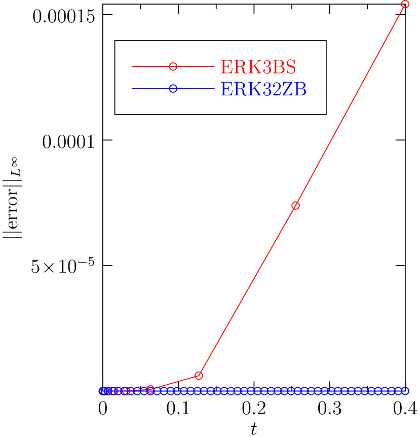
Figure 3: Evolution of the error for (26).

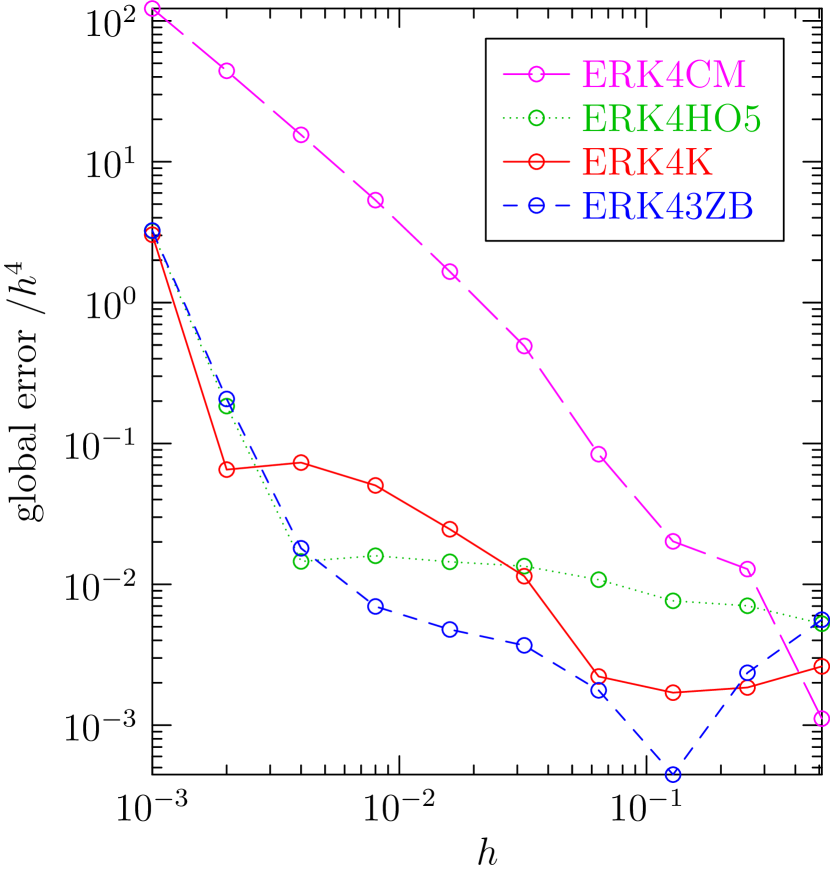
Figure 4: Error vs. timestep in solving (24) with ERK4K, ERK4CM, ERK4HO5, and ERK43ZB at $t=1$.

We say that an adaptive pair is robust if the order of the low-order method is never equal to the order $n$ of the high-order method for any function $G(t)$ with a nonzero $k$th derivative for some $k\in\{0,\ldots n-1\}$.

To construct a robust pair, we recall that each ERK method that satisfies the stiff-order conditions reduces to a Runge–Kutta method that satisfies the classical order conditions of the same order. However, this does not mean that the conditions for an ERK method to be robust reduce when $L=0$ to the conditions for a classical method to be robust. To see this, consider the conditions from Table 4 for a method with four stages to not be stiff-order three:

(21a) $$\frac{a_{31}c_{1}^{2}}{2}+\frac{a_{32}c_{2}^{2}}{2}+\frac{a_{33}c_{3}^{2}}{2} \neq\frac{1}{6},$$

(21b) $$c_{1}^{2}a_{31}J\varphi_{2}(-c_{1}hL)+c_{2}^{2}a_{32}J\varphi_{2}(-c_{2}hL)+c_{3}^{2}a_{33}J\varphi_{2}(-c_{3}hL)$$

$$-c_{1}a_{32}Ja_{11}(-hL)-c_{1}a_{33}Ja_{21}(-hL)-c_{2}a_{33}Ja_{22}(-hL) \neq 0,$$

where, consistent with the weak formulation of  Hochbruck and Ostermann [12], the weight factors $a_{3j}$ are evaluated at $0$. The reason that the ERKBS32 method is not robust is that the equality version of (21b) in fact holds for all $hL$ and any analytic function $f$ (i.e. arbitrary $J$). Since this degeneracy persists for all values of $h$, an adaptive time-stepping method will always fail, no matter how much the time step is adjusted. To guarantee that the second-order estimate will never be third-order for sufficiently small $h$, it is sufficient to ensure as $hL\to 0$ that

(22a) $$\frac{a_{31}c_{1}^{2}}{2}+\frac{a_{32}c_{2}^{2}}{2}+\frac{a_{33}c_{3}^{2}}{2} \neq\frac{1}{6},$$

(22b) $$\frac{1}{2}c_{1}^{2}a_{31}+\frac{1}{2}c_{2}^{2}a_{32}+\frac{1}{2}c_{3}^{2}a_{33}-c_{1}a_{32}a_{11}-c_{1}a_{33}a_{21}-c_{2}a_{33}a_{22} \neq 0.$$

But these are not the same as the classical robustness conditions:

(23a) $$\frac{a_{31}c_{1}^{2}}{2}+\frac{a_{32}c_{2}^{2}}{2}+\frac{a_{33}c_{3}^{2}}{2} \neq\frac{1}{6},$$

(23b) $$\frac{1}{6}-c_{1}a_{32}a_{11}-c_{1}a_{33}a_{21}-c_{2}a_{33}a_{22} \neq 0.$$

For example, if conditions (23) are respected, it is possible that (22b) is violated, which when $L=0$ could lead to the low-order ERK method being third order for some functions $f$. To enforce an ERK method to never be third order, one must respect (22). In the optimization step we therefore need to ensure that the third-order estimate does not satisfy any of the third-order stiff conditions evaluated at $L=0$.

Since we will be advancing the solution using the third-order method, we would like to minimize its error. To achieve this, we perform a second optimization: we want the third-order method to be as close as possible to weakly satisfying the stiff-order four conditions in [12]. Moreover, we also need to ensure that the third-order method, which satisfies the stiff-order three conditions weakly, is as close as possible to satisfying them strongly. This is done in a supplementary Mathematica script [22], which generates the robust exponential $(3,2)$ pair ERK32ZB displayed in Table 9.

Similarly, we constructed a robust exponential $(4,3)$ pair ERK43ZB, displayed in Table 10, by ensuring that the fourth-order method is as close as possible to weakly satisfying the stiff-order five conditions in [16] and as close as possible to satisfying the stiff-order four conditions strongly. As one can imagine, enforcing these demands is not as straightforward as when optimizing classical RK methods. The difficulty lies in the fact that we need to take special care of the arbitrary operators $J$, $K$, $W$, and the bilinear mapping $B$ that appear in some of the stiff-order conditions.

$$\begin{array}[]{c|cccccc}0\\ \frac{1}{2}&\frac{1}{2}\varphi_{1}{\left(-\frac{hL}{2}\right)}\\ \frac{3}{4}&\frac{3}{4}\varphi_{1}{\left(-\frac{3hL}{4}\right)}-a_{11}&\frac{9}{8}\varphi_{2}(-\frac{3hL}{4})+\frac{3}{8}\varphi_{2}(-\frac{hL}{2})\\ \hline\cr 1&\varphi_{1}-a_{21}-a_{22}-a_{23}&\frac{3}{4}\varphi_{2}-\frac{1}{4}\varphi_{3}&\frac{5}{6}\varphi_{2}+\frac{1}{6}\varphi_{3}\\ 1&a_{30}&a_{31}&a_{32}&a_{33}\end{array}$$

$$\varphi_{i} =\varphi_{i}(-hL)$$

$$a_{30} =\frac{29}{18}\varphi_{1}+\frac{7}{6}\varphi_{1}{\left(-\frac{3hL}{4}\right)}+\frac{9}{14}\varphi_{1}{\left(-\frac{hL}{2}\right)}+\frac{3}{4}\varphi_{2}$$

$$+\frac{2}{7}\varphi_{2}{\left(-\frac{3hL}{4}\right)}+\frac{1}{12}\varphi_{2}{\left(-\frac{hL}{2}\right)}-\frac{8083}{420}\varphi_{3}+\frac{11}{30}\varphi_{3}{\left(-\frac{hL}{2}\right)}$$

$$a_{31} =-\frac{1}{9}\varphi_{1}-\frac{1}{6}\varphi_{1}{\left(-\frac{3hL}{4}\right)}-\frac{1}{2}\varphi_{2}$$

$$-\frac{1}{7}\varphi_{2}{\left(-\frac{3hL}{4}\right)}-\frac{1}{3}\varphi_{2}{\left(-\frac{hL}{2}\right)}+\frac{1}{6}\varphi_{3}+\frac{1}{6}\varphi_{3}{\left(-\frac{hL}{2}\right)}$$

$$a_{32} =\frac{2}{3}\varphi_{1}-\frac{1}{2}\varphi_{1}{\left(-\frac{3hL}{4}\right)}-\frac{1}{7}\varphi_{1}{\left(-\frac{hL}{2}\right)}+\frac{1}{3}\varphi_{2}$$

$$-\frac{1}{7}\varphi_{2}{\left(-\frac{3hL}{4}\right)}-\frac{1}{5}\varphi_{3}{\left(-\frac{hL}{2}\right)}$$

$$a_{33} =-\frac{7}{6}\varphi_{1}-\frac{1}{2}\varphi_{1}{\left(-\frac{3hL}{4}\right)}-\frac{1}{2}\varphi_{1}{\left(-\frac{hL}{2}\right)}-\frac{7}{12}\varphi_{2}$$

$$+\frac{1}{4}\varphi_{2}{\left(-\frac{hL}{2}\right)}+\frac{2671}{140}\varphi_{3}-\frac{1}{3}\varphi_{3}{\left(-\frac{hL}{2}\right)}$$

Table 9: ERK32ZB tableau.

$$\begin{array}[]{c|cccccc}0\\ \frac{1}{6}&\frac{1}{6}\varphi_{1}{\left(-\frac{hL}{6}\right)}\\ \frac{1}{2}&\frac{1}{2}\varphi_{1}{\left(-\frac{hL}{2}\right)}-a_{11}&a_{11}\\ \frac{1}{2}&\frac{1}{2}\varphi_{1}{\left(-\frac{hL}{2}\right)}-a_{21}-a_{22}&a_{21}&a_{22}\\ \hline\cr 1&\varphi_{1}-a_{31}-a_{32}-a_{33}&a_{31}&a_{32}&a_{33}\\ 1&\varphi_{1}-\frac{67}{9}\varphi_{2}+\frac{52}{3}\varphi_{3}&8\varphi_{2}-24\varphi_{3}&\frac{26}{3}\varphi_{3}-\frac{11}{9}\varphi_{2}&a_{43}&a_{44}\end{array}$$

$$\varphi_{i} =\varphi_{i}(-hL)$$

$$a_{11} =\frac{3}{2}\varphi_{2}{\left(-\frac{hL}{2}\right)}+\frac{1}{2}\varphi_{2}{\left(-\frac{hL}{6}\right)}$$

$$a_{21} =\frac{19}{60}\varphi_{1}+\frac{1}{2}\varphi_{1}{\left(-\frac{hL}{2}\right)}+\frac{1}{2}\varphi_{1}{\left(-\frac{hL}{6}\right)}$$

$$+2\varphi_{2}{\left(-\frac{hL}{2}\right)}+\frac{13}{6}\varphi_{2}{\left(-\frac{hL}{6}\right)}+\frac{3}{5}\varphi_{3}{\left(-\frac{hL}{2}\right)}$$

$$a_{22} =-\frac{19}{180}\varphi_{1}-\frac{1}{6}\varphi_{1}{\left(-\frac{hL}{2}\right)}-\frac{1}{6}\varphi_{1}{\left(-\frac{hL}{6}\right)}$$

$$-\frac{1}{6}\varphi_{2}{\left(-\frac{hL}{2}\right)}+\frac{1}{9}\varphi_{2}{\left(-\frac{hL}{6}\right)}-\frac{1}{5}\varphi_{3}{\left(-\frac{hL}{2}\right)}$$

$$a_{33} =\varphi_{2}+\varphi_{2}{\left(-\frac{hL}{2}\right)}-6\varphi_{3}-3\varphi_{3}{\left(-\frac{hL}{2}\right)}$$

$$a_{31} =3\varphi_{2}-\frac{9}{2}\varphi_{2}{\left(-\frac{hL}{2}\right)}-\frac{5}{2}\varphi_{2}{\left(-\frac{hL}{6}\right)}+6a_{33}+a_{21}$$

$$a_{32} =6\varphi_{3}+3\varphi_{3}{\left(-\frac{hL}{2}\right)}-2a_{33}+a_{22}$$

$$a_{43} =\frac{7}{9}\varphi_{2}-\frac{10}{3}\varphi_{3},\qquad a_{44}=\frac{4}{3}\varphi_{3}-\frac{1}{9}\varphi_{2}$$

Table 10: ERK43ZB tableau.

As we have already stated, ERK43ZB is a stiff-order four method with a second-last stage yielding a stiff-order three estimate that is guaranteed to never be of higher order. Moreover, the fourth-order estimate in ERK43ZB has minimal error. This has been achieved by minimizing the $L^{2}$ norm of a vector $E_{5}$ whose entries are the coefficients of every term involving $J$, $K$, $W$, the bilinear mapping $B$, $\varphi_{k}(-c_{j}hL)$, and any combination of these operators. For the method ERK43ZB, $E_{5}=1.43838$. By comparison, ERK4HO5 has $E_{5}=6.67545$. This does not mean that the fourth-order estimate in ERK43ZB will do better than ERK4HO5 for every example, but typically it will be more accurate. As pointed out by [9], there is no need to perform such an optimization for the lower-order estimate since it is only used for step-size control.

Accuracy of the higher-order method is not the only front where the embedded ERK method given by [8] falls behind. It is not hard to see that the third-order estimate in ERK43DK weakly satisfies stiff-order condition $6$ in Table 4. Hence, there will exist discretizations for which both estimates will provide a fourth-order approximation to the solution, as seen in Figure 6. This will lead to problems with step-size adjustment, as seen in Figure 6. The same issue arises with the other stiff pair in [8]: the fourth-order estimate in ERK54DK weakly satisfies stiff-order condition $10$ in Table 6. This is also easy to see, noting the similarity between the last stage of the fifth-order method and the last stage of the fourth-order method. There could be further stiff-order five conditions that the fourth-order ERK54DK estimate satisfies, but this is enough to show that this embedded method will also cause step-size adjustment difficulties for some problems. In contrast, by construction, the ERK43ZB method does not suffer from any of these issues. We demonstrate the new embedded exponential pair ERK43ZB for a turbulence shell model in Figure 8.

4 Examples and applications

We now compare popular exponential integrators with our proposed integrator ERK43ZB on the matrix problem in Example 6.2 of [12]:

(24) $$\frac{\partial y}{\partial t}(x,t)-\frac{\partial^{2}y}{\partial x^{2}}(x,t)=\int_{0}^{1}y(\bar{x},t)\,d\bar{x}+\Phi(x,t),$$

for $x\in[0,1]$ and $t\in[0,1]$, subject to homogeneous Dirichlet boundary conditions. The function $\Phi$ is chosen by substituting in the equation the exact solution which is taken to be

(25) $$y(x,t)=x(1-x)e^{t}.$$

This problem can be transformed to a system of ordinary differential equations by performing a centered spatial discretization of the Laplacian term. Hochbruck and Ostermann [12] used the discretized version of (24) with $200$ spatial grid points to demonstrate the order reduction of the Krogstad method ERK4K and the Cox and Matthews method ERK4CM. We replicate their results, while adding the error produced by ERK43ZB, in Figure 4. As in [12], we calculated the matrix $\varphi_{k}$ functions with the help of Padé approximants. The plots show the $L^{2}$-norm of the error at the time $t=1$. They appear different from the plots in the original paper only because we divided the error by $h^{4}$ (since the methods in consideration are supposed to be fourth order), allowing us to examine the constant $C$ in front of $h^{4}$ in the global error. This gives us a better grasp of which among various methods of the same order is better for the given problem.

We now examine the capability of ERK43ZB to adjust the step size as the numerical solution is evolved in order for the error to remain within a specified tolerance. We revisit another example from [12]:

(26) $$\frac{\partial y}{\partial t}(x,t)-\frac{\partial^{2}y}{\partial x^{2}}(x,t)=\frac{1}{1+y(x,t)^{2}}+\Phi(x,t),$$

for $x\in[0,1]$. Again, we discretize in space using $200$ grid points, although this time we continue the time integration from $t_{0}=0$ to $t_{n}=3$ in order to show how ERK43ZB performs over a longer time. The exact solution of (26) is again taken to be

(27) $$y(x,t)=x(1-x)e^{t}$$

and the term $\Phi(x,t)$ is calculated by substituting the exact solution into the equation. Our plan was to compare our stiff $(4,3)$ pair with the stiff $(4,3)$ pair ERK43DK, but as we explained at the end of the previous chapter, the third-order estimate in ERK43DK is actually fourth order for some problems, as shown in Figure 6. This makes it falsely conclude that the difference between its fourth-order estimate and its (supposed) third-order estimate is extremely small, misleading the time step adjustment algorithm into adopting a time step that is too large to stay within the specified global error. In Figure 6 we show the evolution of the $L^{\infty}$ error over the time interval $[0,3]$. We note that ERK43ZB successfully adapts the time step to keep the error small, whereas ERK43DK erroneously continues to increase the time step without bound!

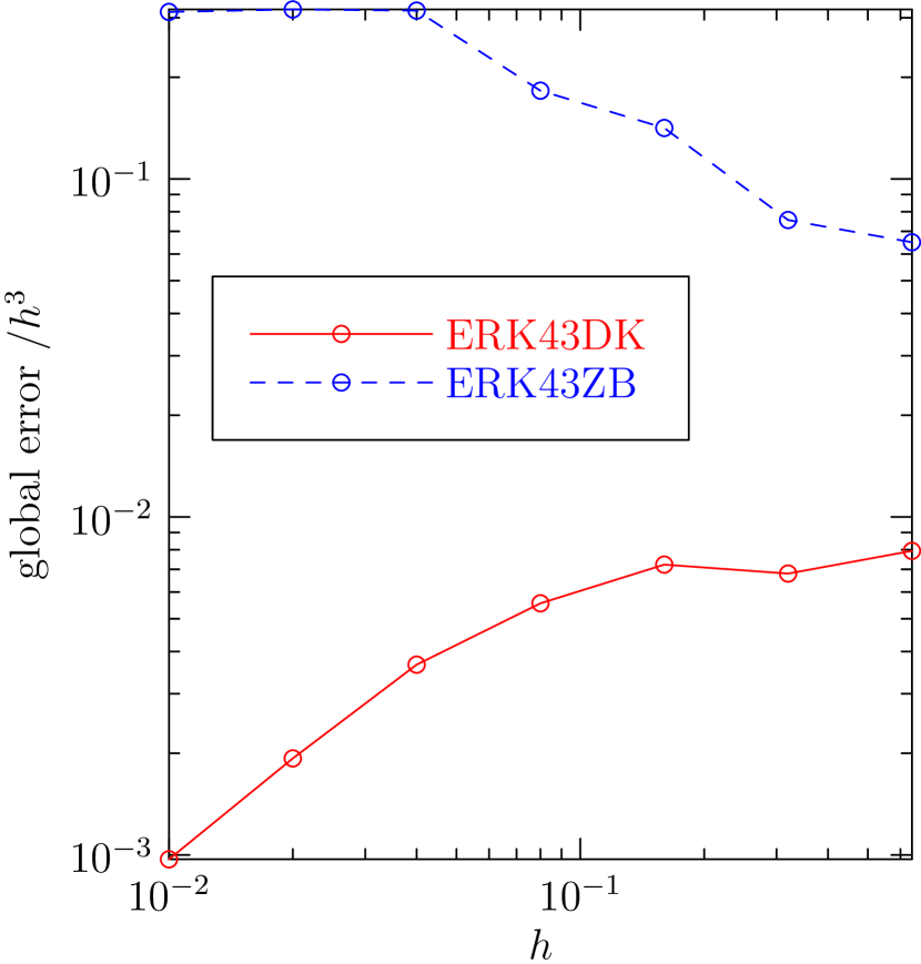
Figure 5: Error vs. time step of the third-order estimates for (26) at $t=3$.

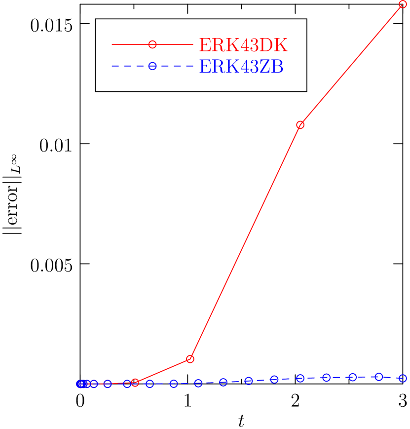
Figure 6: Evolution of the error for (26).

Perhaps the best way to showcase the ability of ERK43ZB to adjust the step size over the course of a long time integration is by trying to approximate a solution that is periodic in time. Consider 26 for $x\in[0,1]$ with $\Phi$ chosen so that the exact solution is $y(x,t)=10(1-x)x(1+\sin t)+2$, discretized using $200$ grid points and integrated in time from $t=0$ to $t=30$. In Figure 8 we plot the $L^{\infty}$ norm of the error at each adaptive time step. The classical Cash–Karp (5,4) Runge–Kutta embedded pair is much less efficient for this problem: it requires an average timestep roughly 20000 times smaller than that used by ERK43ZB.

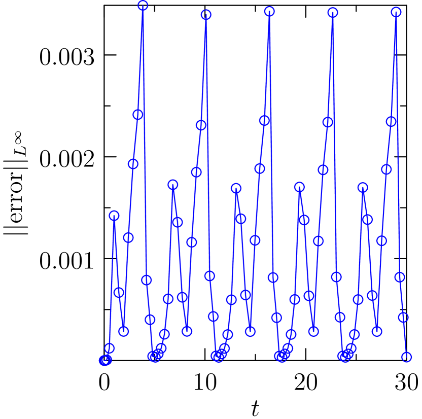
Figure 7: Evolution of the error for (26) with $\Phi$ chosen so that the exact solution is $y(x,t)=10(1-x)x(1+\sin t)+2$.

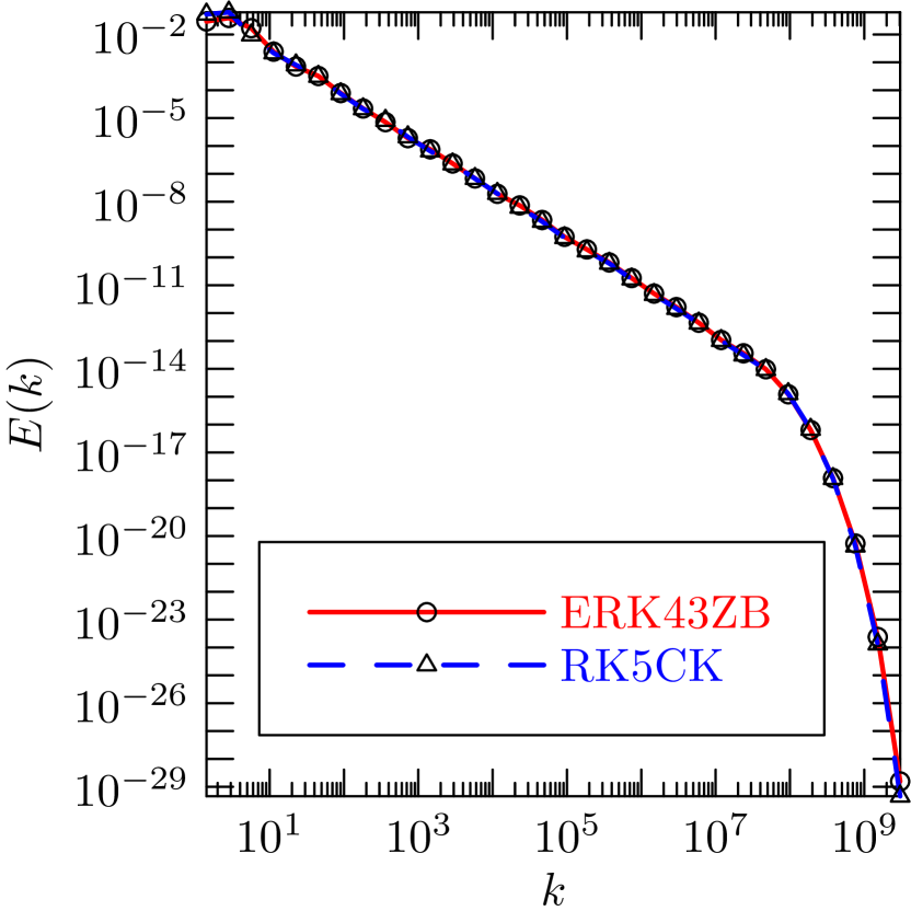
Figure 8: Time-averaged energy spectrum for the GOY shell model from $t=5$ to $t=10$ predicted by ERK43ZB and the Cash–Karp (5,4) Runge–Kutta embedded pair RK5CK.

In Figure 8, we compare the ERK43ZB embedded pair to the classical Cash–Karp (5,4) Runge-Kutta pair RK5CK for a forced-dissipative simulation of the Gledzer–Ohkitani–Yamada turbulence shell model [11, 19, 21, 20], using an adaptive time step, with 32 shells, unit white-noise energy injection and Laplacian dissipation coefficient $10^{-11}$. We benchmarked these algorithms on a single thread of an 5.2GHz Intel i9-12900K processor on an ASUS ROG Strix Z690-F motherboard with 5GHz DDR5 memory. The exponential method required 579 seconds, with a mean time step of $1.39\times 10^{-7}$ seconds, while the classical method required 2098 seconds, with a mean time step of $3.89\times 10^{-8}$ seconds. Applying an exponential integrator to this problem, which suffers from both linear and nonlinear stiffness, led to a speedup of $3.62$.

5 Conclusion

Exponential integrators are well suited to solving linearly stiff ordinary differential equations. These explicit methods can achieve high accuracy with relatively large step sizes. In the limit of vanishing linearity, they reduce to classical discretizations. In this work, we are specifically interested in robust embedded exponential Runge–Kutta pairs for adaptive time stepping. To date, no robust adaptive exponential integrators beyond third order have been presented in the literature. For example, we have seen that the exponential version ERKBS32 of the $(3,2)$ embedded Bogacki–Shampine Runge–Kutta pair [2], as well as the $(4,3)$ ERK43DK and $(5,4)$ ERK54DK methods in [8], are not robust.

Symbolic algebra software was used to derive robust exponential Runge–Kutta (3,2) and (4,3) embedded pairs ERK32ZB and ERK43ZB; they were optimized to minimize the error of the high-order estimate. These methods maintain their design orders when applied to the examples that Hochbruck and Ostermann used to demonstrate stiff order reduction [12]; they also avoid the step-size adjustment issues observed with ERK43DK in Figure 6. To illustrate a practical application of embedded exponential pairs, we showed that the (4,3) exponential pair ERK43ZB runs over three times faster than a classical (5,4) pair when applied to a shell model of three-dimensional turbulence exhibiting both linear and nonlinear stiffness.

References

- [1] S. Balac and F. Mahé, Embedded Runge-Kutta scheme for step-size control in the interaction picture method, Computer Physics Communications, 184 (2013), pp. 1211–1219.
- [2] J. C. Bowman, C. R. Doering, B. Eckhardt, J. Davoudi, M. Roberts, and J. Schumacher, Links between dissipation, intermittency, and helicity in the GOY model revisited, Physica D, 218 (2006), pp. 1–10.
- [3] J. P. Boyd, Chebyshev and Fourier spectral methods, Dover, 2001.
- [4] J. C. Butcher, On fifth and sixth order explicit Runge-Kutta methods: order conditions and order barriers, Canadian Applied Mathematics Quarterly, 17 (2009), pp. 433–445.
- [5] J. R. Cash and A. H. Karp, A variable order Runge-Kutta method for initial value problems with rapidly varying right-hand sides, ACM Transactions on Mathematical Software (TOMS), 16 (1990), pp. 201–222.
- [6] J. Certaine, The solution of ordinary differential equations with large time constants, Mathematical methods for digital computers, 1 (1960), pp. 128–132.
- [7] S. Cox and P. Matthews, Exponential time differencing for stiff systems, J. Comp. Phys., 176 (2002), pp. 430–455.
- [8] X. Ding and S. Kang, Stepsize-adaptive integrators for dissipative solitons in cubic-quintic complex ginzburg-landau equations, arXiv preprint arXiv:1703.09622, (2017).
- [9] J. R. Dormand and P. J. Prince, A family of embedded Runge-Kutta formulae, Journal of computational and applied mathematics, 6 (1980), pp. 19–26.
- [10] E. Fehlberg, Klassische Runge-Kutta-formeln fünfter und siebenter ordnung mit schrittweiten-kontrolle, Computing, 4 (1969), pp. 93–106.
- [11] E. B. Gledzer, System of hydrodynamic type admitting two quadratic integrals of motion, Sov. Phys. Dokl., 18 (1973), pp. 216–217.
- [12] M. Hochbruck and A. Ostermann, Explicit exponential Runge–Kutta methods for semilinear parabolic problems, SIAM J. Numer. Anal., 43 (2005), pp. 1069–1090.
- [13] A.-K. Kassam and L. N. Trefethen, Fourth-order time-stepping for stiff pdes, SIAM J. Sci. Comput., 26 (2005), pp. 1214–1233.
- [14] S. Krogstad, Generalized integrating factor methods for stiff pdes, Journal of Computational Physics, 203 (2005), pp. 72–88.
- [15] J. D. Lambert, Numerical methods for ordinary differential systems: the initial value problem, John Wiley & Sons, Inc., 1991.
- [16] V. T. Luan and A. Ostermann, Explicit exponential Runge-Kutta methods of high order for parabolic problems, Journal of Computational and Applied Mathematics, 256 (2014), pp. 168–179.
- [17] M. Tokman and J. Loffeld, Efficient design of exponential-Krylov integrators for large scale computing, Procedia Computer Science, 1 (2010), pp. 229–237.
- [18] P. Whalen, M. Brio, and J. V. Moloney, Exponential time-differencing with embedded Runge-Kutta adaptive step control, Journal of Computational Physics, 280 (2015), pp. 579–601.
- [19] M. Yamada and K. Ohkitani, Lyapunov spectrum of a chaotic model of three-dimensional turbulence, J. Phys. Soc. Jap., 56 (1987), pp. 4210–4213.
- [20] M. Yamada and K. Ohkitani, Lyapunov spectrum of a model of two-dimensional turbulence, Phys. Rev. Lett., 60 (1988), p. 983.
- [21] M. Yamada and K. Ohkitani, Asymptotic formulas for the lyapunov spectrum of fully developed shell model turbulence, Phys. Rev. E, 57 (1998), pp. R6257–R6260, https://doi.org/10.1103/PhysRevE.57.R6257.
- [22] T. Zoto and J. C. Bowman, 2023, https://github.com/stiffode/expint (accessed 2023-03-25).
- [23] T. Zoto and J. C. Bowman, Schur decomposition for stiff differential equations, SIAM J. Sci. Comput., (2023). to be submitted.