Fast randomized entropically regularized
semidefinite programming

Abstract

We develop a practical approach to semidefinite programming (SDP) that includes the von Neumann entropy, or an appropriate variant, as a regularization term. In particular we solve the dual of the regularized program, demonstrating how a carefully chosen randomized trace estimator can be used to estimate dual gradients effectively. We also introduce specialized optimization approaches for common SDP, specifically SDP with diagonal constraint and the problem of the determining the spectral projector onto the span of extremal eigenvectors. We validate our approach on such problems with applications to combinatorial optimization and spectral embedding.

1 Introduction

In this work we are interested in the solution of semidefinite programs (SDPs) of the form

$$\underset{X\in\mathbb{R}^{n\times n}}{\text{minimize}}\quad \mathrm{Tr}[CX]$$

subject to $$X\succeq 0,\ \mathrm{Tr}\left[A_{k}X\right]=b_{k},\ k=1,\ldots,m.$$

A major obstacle in semidefinite programming is that enforcing the semidefinite constraint on an $n\times n$ matrix $X$ in general requires $\sim n^{3}$ operations. This can be understood intuitively by realizing that detecting semidefiniteness (i.e., checking whether all eigenvalues are nonnegative) essentially involves computing a complete spectrum.

Major progress in avoiding $n^{3}$ scaling has been made in the case when the optimal solution $X^{\star}$ is of rank $k\ll n$. In this case, many specialized approaches are able to achieve per-iteration complexity of $O(nk^{2})$. These include the Burer-Monteiro / SDPLR method [4] and alternative manifold-constrained optimization approaches [3], as well as the randomized approach SketchyCGAL [23].

In this work we are mainly interested in settings where the numerical rank is high enough such that $O(nk^{2})$ scaling is prohibitive, and we pursue algorithms that do not depend on any rank truncation. However, our regularization approach also smooths the problem and could possibly yield a convergence advantage even for low-rank problems, provided that approximation is acceptable.

Inspired by the success of entropic regularization [6] of the Kantorovich problem of optimal transport, which is a linear program, we pursue the regularization of SDPs by the von Neumann entropy, as well as other variants as appropriate. Regularization by the von Neumann entropy has been considered in [14, 19, 18] and moreover can be viewed as fundamental to the perspective of quantum statistical mechanics at finite temperature (cf. [15] for mathematical introduction). We will develop an appropriate theory of duality which shall be of no surprise from a physicist’s point of view, but which to our knowledge has not been exploited for the purpose of fast solution of SDPs.

In contrast to the situation of entropically regularized optimal transport, the duality theory of entropically regularized SDPs does not immediately suggest any algorithmic treatment. Indeed, the dual gradients require the computation of certain matrix traces that cannot be computed exactly in less than $O(n^{3})$ time.

The idea for trace estimation is based on Hutchinson’s trace estimator [11, 17], with a ‘square root’ trick that has also been applied in the context of Gaussian process regression (GPR) [16]. Unlike the context of GPR in which the trick requires expensive matrix-vector multiplications by the square root of the kernel matrix, in our context the square root trick imposes no additional computational burden relative to the ‘default’ strategy.

We focus on two problem types of interest. The first type is that of SDPs with diagonal constraint, which include the Goemans-Williamson relaxation of the Max-Cut problem [9]. For SDPs with this structure we introduce a specialized optimization approach that takes some loose inspiration from matrix scaling [6] and can be viewed as solving a sequence of minorized dual problems.

The second type is the SDP formulation of the problem of computing the spectral projector onto the span of extremal eigenvectors. Here we use the binary von Neumann entropy as a regularizer, which connects to the theory of single-particle fermionic statistical mechanics (again cf. [15] for mathematical introduction), and our specialized optimization approach is simply Newton’s method, with updates computed by appropriate randomized trace estimation. We demonstrate an application to graph spectral embedding [20, 21].

For fixed value of the regularization parameter, the per-iteration cost of our algorithms scales according to the cost of matrix-vector multiplication by the cost and constraint matrices $C$ and $A_{1},\ldots,A_{m}$, yielding $O(n)$ per-iteration scaling in our applications for graphs of bounded degree. Empirically we find that for the problem families of interest, when the regularization parameter is fixed, the optimization converges in $O(1)$ iterations.

We conclude the introduction with an outline of the paper. In Section 2 we introduce the general framework of entropic regularization and duality. In Section 3 we describe the trace estimation procedure needed in our algorithms, which is equipped with rigorous concentration bounds. In Section 4 we describe specialized optimization approaches for problems of interest. In Section 5 we discuss applications to the Max-Cut problem and spectral clustering and present numerical experiments.

2 Entropic regularization of SDP

Consider the general semidefinite program

$$\underset{X\in\mathbb{R}^{n\times n}}{\text{minimize}}\quad \mathrm{Tr}[CX]$$ (2.1)

subject to $$X\succeq 0,$$

$$\mathrm{Tr}\left[\mathbf{A}X\right]=\mathbf{b}.$$

Here $\mathbf{A}=(A_{1},\ldots,A_{m})\in\mathbb{R}^{m\times(n\times n)}$ indicates a vector of matrices, which together with $\mathbf{b}=(b_{1},\ldots,b_{m})\in\mathbb{R}^{m}$, specifies $m$ linear equality constraints $\mathrm{Tr}[A_{i}X]=b_{i}$, $i=1,\ldots,m$, on the optimization variable $X$. We can always assume that the cost matrix $C\in\mathbb{R}^{n\times n}$ is symmetric by symmetrizing if necessary, which does not alter the objective. We moreover assume without loss of generality that $A_{1},\ldots,A_{m}$ are symmetric as they too can be symmetrized without altering the expression $\mathrm{Tr}[\mathbf{A}X]$.

Algorithmically we shall only require access to the cost matrix $C$ and the constraint matrices $A_{i}$ via matrix-vector multiplications (matvecs). Thus in the case where the cost and constraint matrices are sparse or otherwise structured, fast matvecs can be easily exploited.

More generally we can consider complex-valued $C,\mathbf{A},\mathbf{b}$ and Hermitian positive definite optimization variable $X$, where $C$ can be assumed to be Hermitian, and the objective is replaced by $\mathrm{Re}\left(\mathrm{Tr}[CX]\right)$. For simplicity we restrict our discussion to the real case.

Consider regularizing the problem by the addition of a von Neumann entropy term

$$S(X):=\mathrm{Tr}\left[X\log X-X\right]$$

as follows:

$$\underset{X\in\mathbb{R}^{n\times n}}{\text{minimize}}\quad \mathrm{Tr}[CX]+\beta^{-1}S(X)$$

subject to $$\mathrm{Tr}\left[\mathbf{A}X\right]=\mathbf{b}.$$

Here $\beta\in(0,\infty)$ carries the physical interpretation of an inverse temperature in quantum statistical mechanics, and the domain of $S(X)$ is implicitly understood to be the positive definite cone $\{X\succ 0\}$.

2.1 Duality

Introducing a Lagrange multiplier $\boldsymbol{\lambda}\in\mathbb{R}^{m}$, we obtain the minimax problem for the suitable Lagrangian

$$\min_{X\in\mathbb{R}^{n\times n}}\max_{\boldsymbol{\lambda}\in\mathbb{R}^{m}}\mathcal{L}(X,\boldsymbol{\lambda}),$$

where

$$\mathcal{L}(X,\boldsymbol{\lambda}):=\ \mathrm{Tr}[CX]+\beta^{-1}S(X)+\boldsymbol{\lambda}\cdot\left(\mathbf{b}-\mathrm{Tr}[\mathbf{A}\cdot X]\right)$$

$$=\ \mathrm{Tr}\left[\left(C-\boldsymbol{\lambda}\cdot\mathbf{A}\right)X\right]+\beta^{-1}S(X)+\mathbf{b}\cdot\boldsymbol{\lambda}.$$

Minimization over $X$ yields optimizer

$$X=e^{-\beta(C-\boldsymbol{\lambda}\cdot\mathbf{A})},$$

and the dual objective $g(\boldsymbol{\lambda})$ is then computed as

$$g(\boldsymbol{\lambda}):=\max_{X}\mathcal{L}(X,\boldsymbol{\lambda})=\mathbf{b}\cdot\boldsymbol{\lambda}-\beta^{-1}\mathrm{Tr}\left[e^{-\beta(C-\boldsymbol{\lambda}\cdot\mathbf{A})}\right],$$

yielding the dual problem

$$\underset{\boldsymbol{\lambda}\in\mathbb{R}^{m}}{\text{maximize}}\quad \mathbf{b}\cdot\boldsymbol{\lambda}-\beta^{-1}\mathrm{Tr}\left[e^{-\beta(C-\boldsymbol{\lambda}\cdot\mathbf{A})}\right],$$

in which the second term of the objective carries the interpretation of the quantum Gibbs free energy.

When a dual solution $\boldsymbol{\lambda}^{\star}$ is obtained, the primal solution $X^{\star}=X(\boldsymbol{\lambda}^{\star})$, where

$$X(\boldsymbol{\lambda}):=e^{-\beta(C-\boldsymbol{\lambda}\cdot\mathbf{A})}$$ (2.2)

carries the interpretation of an unnormalized quantum density operator.

2.2 Dual gradients

To solve the dual optimization problem via first-order methods, we are motivated to compute the gradient of $g(\boldsymbol{\lambda})$. These can be obtained analytically as

$$\nabla g(\boldsymbol{\lambda})=\nabla_{\boldsymbol{\lambda}}\mathcal{L}(X(\boldsymbol{\lambda}),\boldsymbol{\lambda})=\mathbf{b}-\mathrm{Tr}\left[\mathbf{A}X(\boldsymbol{\lambda})\right].$$ (2.3)

It is inefficient to evaluate the gradient directly, since forming the matrix exponential exactly requires $O(n^{3})$ operations. We will discuss in Section 3 how to estimate traces of the form appearing in (2.3) using only matvecs by the cost and constraint matrices.

2.3 The case of diagonal constraint

Of particular interest is the case where $A_{i}=e_{i}e_{i}^{\top}$, $i=1,\ldots,n$, i.e., $m=n$. In the case the primal SDP takes the form

$$\underset{X\in\mathbb{R}^{n\times n}}{\text{minimize}}\quad \mathrm{Tr}[CX]$$ (2.4)

subject to $$X\succeq 0,$$

$$\mathrm{diag}(X)=\mathbf{b},$$

the dual regularized SDP takes the form

$$\underset{\boldsymbol{\lambda}\in\mathbb{R}^{m}}{\text{maximize}}\quad\mathbf{b}\cdot\boldsymbol{\lambda}-\beta^{-1}\mathrm{Tr}\left[e^{-\beta(C-\mathrm{diag}(\boldsymbol{\lambda}))}\right],$$

and the dual gradients are

$$\nabla g(\boldsymbol{\lambda})=\mathbf{b}-\mathrm{diag}\left[X(\boldsymbol{\lambda})\right].$$

Hence computing the dual gradients requires the estimation of the diagonal of a positive definite matrix, which is in particular presented as a matrix exponential.

2.4 Binary-entropic regularization

Although (2.1) is the general form of an SDP, many specific SDPs can only be reduced to this form via the introduction of additional optimization variables and a mess of dense equality constraints. We provide an example of how the framework of entropically regularized SDP can extend to another setting of interest without sacrificing conceptual clarity and algorithmic efficiency. Consider the SDP

$$\underset{X\in\mathbb{R}^{n\times n}}{\text{minimize}}\quad \mathrm{Tr}[CX]$$ (2.5)

subject to $$0\preceq X\preceq I,$$

$$\mathrm{Tr}\left[\mathbf{A}X\right]=\mathbf{b},$$

which differs only from (2.1) via the inclusion of an upper bound on $X$ in the Loewner ordering.

In this setting, we may instead regularize by the binary von Neumann entropy, which generalizes the ordinary binary entropy to the matrix case:

$$S_{\mathrm{bin}}(X):=\mathrm{Tr}[X\log X]+\mathrm{Tr}\log[(I-X)\log(I-X)].$$

The domain of $S_{\mathrm{bin}}$ is understood to be $\{0\prec X\prec I\}$, the set of all symmetric matrices with eigenvalues strictly between $0$ and $1$.

In this setting the Lagrangian reads as

$$\mathcal{L}(X,\boldsymbol{\lambda})=\ =\ \mathrm{Tr}\left[\left(C-\boldsymbol{\lambda}\cdot\mathbf{A}\right)X\right]+\beta^{-1}S_{\mathrm{bin}}(X)+\mathbf{b}\cdot\boldsymbol{\lambda},$$

whose primal optimizer for fixed $\boldsymbol{\lambda}$ is

$$X(\boldsymbol{\lambda})=\left[I+e^{\beta\left(C-\boldsymbol{\lambda}\cdot\mathbf{A}\right)}\right]^{-1}=F_{\beta}\left(C-\boldsymbol{\lambda}\cdot\mathbf{A}\right),$$ (2.6)

where

$$F_{\beta}(x)=\frac{1}{1+e^{\beta x}}=\frac{1}{2}\left(1-\tanh(\beta x/2)\right)$$

is the Fermi-Dirac function at inverse temperature $\beta$.

Some computation reveals that the dual objective can be written

$$g(\boldsymbol{\lambda})=\mathbf{b}\cdot\boldsymbol{\lambda}+\beta^{-1}\mathrm{Tr}\left[\log\left(I+e^{-\beta(C-\boldsymbol{\lambda}\cdot\mathbf{A})}\right)\right],$$

in which the last term can be interpreted as a fermionic free energy. The dual gradient is once again given by the expression

$$\nabla g(\boldsymbol{\lambda})=\nabla_{\boldsymbol{\lambda}}\mathcal{L}(X(\boldsymbol{\lambda}),\boldsymbol{\lambda})=\mathbf{b}-\mathrm{Tr}\left[\mathbf{A}X(\boldsymbol{\lambda})\right],$$

where now $X(\boldsymbol{\lambda})$ carries a different interpretation, after (2.6).

.

2.5 Extremal eigenvalue problem

A special case of (2.5) of particular interest is the

$$\underset{X\in\mathbb{R}^{n\times n}}{\text{minimize}}\quad \mathrm{Tr}[CX]$$ (2.7)

subject to $$0\preceq X\preceq I,$$

$$\mathrm{Tr}\left[X\right]=k,$$

which is an SDP formulation of the problem of finding the lowest $k$ eigenvectors of a symmetric matrix $C$. Indeed, the optimal solution is recovered as

$$X^{\star}=\sum_{i=1}^{k}u_{i}u_{i}^{\top},$$

where $(\lambda_{i},u_{i})$, $i=1,\ldots,n$, are the eigenpairs of $C$, ordered $\lambda_{1}\leq\cdots\leq\lambda_{n}$, assuming we have a gap $\lambda_{k}<\lambda_{k+1}$ between the $k$-th and $(k+1)$-th eigenvalues.

The format (2.5) is recovered by taking $m=1$, $A_{1}=I$, and $b_{1}=k$. In this case the Lagrange multiplier is a scalar carrying the interpretation of a chemical potential, hence we shall denote it by $\mu$, and the dual objective can be written

$$g(\mu)=k\mu+\beta^{-1}\mathrm{Tr}\left[\log\left(1+e^{-\beta(C-\mu I)}\right)\right],$$

and the derivative is

$$g^{\prime}(\mu)=k-\mathrm{Tr}\left[X(\mu)\right].$$ (2.8)

In fact in this case, the second derivative admits a simple expression, owing to the fact that the constraint matrix $I$ commutes with the cost matrix $C$:

$$g^{\prime\prime}(\mu)=-\beta\,\mathrm{Tr}\left[\frac{e^{\beta(C-\mu I)}}{\left[I+e^{\beta(C-\mu I)}\right]^{2}}\right],$$

which can be rewritten conveniently as

$$g^{\prime\prime}(\mu)=-\beta\,\mathrm{Tr}\left[\left(I-X(\mu)\right)X(\mu)\right],$$ (2.9)

where we recall $X(\mu)=\left[I+e^{\beta(C-\mu I)}\right]^{-1}$.

3 Trace estimation

It is inefficient to exactly construct the entire matrix $X(\boldsymbol{\lambda})$ following (2.1). We could instead pursue a randomized approach for computing the gradient (2.3) directly without forming $X(\boldsymbol{\lambda})$.

Instead, we will only ever require the capacity to perform matvecs by $Y(\boldsymbol{\lambda}):=X^{1/2}(\boldsymbol{\lambda})$. In fact, we only require the capacity to perform matvecs by any $Y(\boldsymbol{\lambda})$ achieving the factorization $X(\boldsymbol{\lambda})=Y(\boldsymbol{\lambda})Y(\boldsymbol{\lambda})^{\top}$. However, given the presentation of $X(\boldsymbol{\lambda})$ as a matrix function, the most straightforward practical choice of factorization available is furnished by $Y(\boldsymbol{\lambda})=X^{1/2}(\boldsymbol{\lambda})$, and we will restrict our discussion to this choice.

In the case (2.2) of ordinary entropic regularization we have

$$Y(\boldsymbol{\lambda})=e^{-\frac{\beta}{2}(C-\boldsymbol{\lambda}\cdot\mathbf{A})},$$ (3.1)

while in the case (2.6) of binary entropic regularization we have

$$Y(\boldsymbol{\lambda})=F_{\beta}^{1/2}(C-\boldsymbol{\lambda}\cdot\mathbf{A}),$$ (3.2)

where $F_{\beta}^{1/2}$ denotes the square root of the Fermi-Dirac function

$$F_{\beta}^{1/2}(x)=\frac{1}{\sqrt{1+e^{\beta x}}}.$$ (3.3)

Note that in either case, $Y(\boldsymbol{\lambda})$ presents as a matrix function of $C-\boldsymbol{\lambda}\cdot\mathbf{A}$, which is no more difficult to deal with computationally than $X(\boldsymbol{\lambda})$ itself.

The problem of estimating the diagonal of a matrix $X$ using only matvecs by $X$ has been considered in [2], for example, using a Hutchinson-type estimator. The variance of this estimator, however, depends on the locality of the matrix whose diagonal is to be estimated. By using a Hutchinson-type estimator that instead relies on matvecs by the square root matrix, the variance is guaranteed to be improved [16] for all traces $\mathrm{Tr}[\mathbf{A}X]$. In the case of diagonal estimation, as we shall see, the diagonal entries can in fact be recovered with relative variance that is universal. In the setting of [16], one downside of the square root approach is that matvecs by the square root are more expensive than matvecs by $X$. In our setting, there is essentially no difference in cost as both must be constructed using similar matrix function techniques.

3.1 Estimator

To derive our estimator, compute

$$\mathrm{Tr}[\mathbf{A}X(\boldsymbol{\lambda})] =\mathrm{Tr}[Y(\boldsymbol{\lambda})\mathbf{A}Y(\boldsymbol{\lambda})]$$

$$=\mathbb{E}_{z\sim\mathcal{N}(0,I)}\left(z^{\top}Y(\boldsymbol{\lambda})\mathbf{A}Y(\boldsymbol{\lambda})z\right)$$

$$=\mathbb{E}_{z\sim\mathcal{N}(0,I)}\left(\left[Y(\boldsymbol{\lambda})z\right]^{\top}\mathbf{A}\left[Y(\boldsymbol{\lambda})z\right]\right).$$

This equation suggests the unbiased estimator

$$\mathbf{a}^{(N)}(\boldsymbol{\lambda}):=\frac{1}{N}\sum_{i=1}^{N}\left[Y(\boldsymbol{\lambda})z^{(i)}\right]^{\top}\mathbf{A}\left[Y(\boldsymbol{\lambda})z^{(i)}\right]$$ (3.4)

for $\mathrm{Tr}[\mathbf{A}X(\boldsymbol{\lambda})]$, where $z^{(i)}$, $i=1,\ldots,N$, are independent and identically distributed according to the standard normal distribution $\mathcal{N}(0,I)$.

It is possible more generally to adopt as the distribution for the $z^{(i)}$ any distribution yielding independent entries of unit variance, such as the Rademacher distribution taking values in $\{\pm 1\}$. For simplicity, we restrict our practical attention to the Gaussian case.

Note for concreteness that in the case of the diagonal constraint (where $m=n$ and $A_{k}=e_{k}e_{k}^{\top}$, $k=1,\ldots,n$), we can write

$$\mathbf{a}^{(N)}(\boldsymbol{\lambda})=\frac{1}{N}\sum_{i=1}^{N}\left[Y(\boldsymbol{\lambda})z^{(i)}\right]^{\odot 2},$$

where $u^{\odot 2}$ indicates the entrywise second power of $u$. If we let $Z=[z^{(1)}\,\cdots\,z^{(N)}]\in\mathbb{R}^{n\times N}$, we can more compactly write

$$\mathbf{a}^{(N)}(\boldsymbol{\lambda})=\frac{1}{N}\left[Y(\boldsymbol{\lambda})Z\right]^{\odot 2}\,\mathbf{1}_{N},$$ (3.5)

where $\mathbf{1}_{N}\in\mathbb{R}^{N}$ is the vector of all ones.

3.2 Covariance and concentration inequalities

In this section let us fix $X=X(\boldsymbol{\lambda})$, $Y=Y(\boldsymbol{\lambda})$, and $\mathbf{a}^{(N)}=\mathbf{a}^{(N)}(\boldsymbol{\lambda})$ for notational simplicity.

For $z\sim N(0,I)$, we have

$$\mathbb{E}[(Yz)^{\top}\mathbf{A}(Yz)]=\mathrm{Tr}[\mathbf{A}X],$$

and moreover it can be readily verified via Wick’s theorem, which yields the identity $\mathbb{E}[z_{i}z_{j}z_{k}z_{l}]=\delta_{ij}\delta_{kl}+\delta_{ik}\delta_{il}+\delta_{il}\delta_{jk}$, that the covariance of $(Yz)^{\top}\mathbf{A}(Yz)\in\mathbb{R}^{m}$ is given by

$$\Sigma:=\mathrm{Cov}[(Yz)^{\top}\mathbf{A}(Yz)]=\left(2\,\mathrm{Tr}[A_{i}XA_{j}X]\right)_{i,j=1,\ldots,m}.$$

Therefore the mean and covariance of our estimator $\mathbf{a}^{(N)}$ can be recovered as

$$\mathbb{E}[\mathbf{a}^{(N)}]=\mathrm{Tr}[\mathbf{A}X],\quad\mathrm{Cov}(\mathbf{a}^{(N)})=N^{-1}\Sigma.$$

We moreover have the following concentration bounds on the estimator, applicable for more general choice of the distribution of the $z^{(i)}$:

Proposition 1.

Let $\delta\in(0,1/2]$, and suppose that $z^{(i)},i=1,\ldots,N$ are i.i.d. with entries that are themselves i.i.d. sub-Gaussian random variables with a constant sub-Gaussian parameter, mean zero, and unit variance. There exist constants $c,C>0$ such that if $N>c\log\left(\frac{m}{\delta}\right)$, then with probability at least $1-\delta$, the inequality

$$|a_{i}^{(N)}(\boldsymbol{\lambda})-\mathrm{Tr}\left[A_{i}X(\boldsymbol{\lambda})\right]|\leq C\sqrt{\log\left(\frac{m}{\delta}\right)}\ \sqrt{\frac{\mathrm{Tr}[A_{i}XA_{i}X]}{N}}$$

holds for all $i=1,\ldots,m$.

In the case $\mathbf{A}=(e_{1}e_{1}^{\top},\ldots,e_{n}e_{n}^{\top})$ yielding the SDP with diagonal constraint (2.4), it follows that under the same conditions,

$$\frac{\left\|\mathbf{a}^{(N)}(\boldsymbol{\lambda})-\mathrm{diag}\left[X(\boldsymbol{\lambda})\right]\right\|_{2}}{\left\|\mathrm{diag}\left[X(\boldsymbol{\lambda})\right]\right\|_{2}}\leq C\sqrt{\frac{\log\left(\frac{n}{\delta}\right)}{N}}.$$

Remark 2.

Note that the second statement provides a bound on the relative error of the diagonal estimator that is universal apart from logarithmic dependence on $n$. Unlike the estimator of [2], the error does not depend on locality of $X$.

Proof.

The first statement results from direct application of Lemma 2.1 of [17] to the Hutchinson estimator for each of $YA_{i}Y$, $i=1,\ldots,m$, together with the union bound over the $m$ separate traces.

Note that the first statement implies that

$$\left\|\mathbf{a}^{(N)}(\boldsymbol{\lambda})-\mathrm{diag}\left[X(\boldsymbol{\lambda})\right]\right\|_{2}\leq C\sqrt{\log\left(\frac{m}{\delta}\right)}\ \sqrt{\frac{\sum_{i=1}^{m}\mathrm{Tr}[A_{i}XA_{i}X]}{N}},$$

and the second statement follows immediately in the case $\mathbf{A}=(e_{1}e_{1}^{\top},\ldots,e_{n}e_{n}^{\top})$. ∎

3.3 Matvecs

Several pieces remain in the specification of a concrete algorithm for entropically regularized semidefinite programming. First we must explain how to perform matvecs by $Y(\boldsymbol{\lambda})$.

Observe that in the basic case (3.1), $Y(\boldsymbol{\lambda})=e^{-\beta(C-\boldsymbol{\lambda}\cdot\mathbf{A})}$ is defined as a matrix exponential of a matrix $C-\boldsymbol{\lambda}\cdot\mathbf{A}$ by which matvecs are assumed to be efficient, since they reduce to matvecs by the cost and constraint matrices. In many cases of interest, $C-\boldsymbol{\lambda}\cdot\mathbf{A}$ is in fact a sparse matrix with $O(n)$ nonzero entries. Therefore we apply the algorithm of [1] which lifts a matvec routine for a matrix to a matvec routine for its exponential. This algorithm is based on splitting the exponential into a product of exponentials closer to the identity, which are in turn approximated by a Taylor series.

In the case of (3.2), $Y(\boldsymbol{\lambda})=F_{\beta}^{1/2}(C-\boldsymbol{\lambda}\cdot\mathbf{A})$ is furnished as a more complicated matrix function of the same matrix. Recall that $F_{\beta}^{1/2}$ is the square root of the Fermi-Dirac function, defined as in (3.3). For this matrix function, no specialized algorithm such as [1] is available, so given lower and upper bounds on the spectrum of $C-\boldsymbol{\lambda}\cdot\mathbf{A}$, we simply approximate $F_{\beta}^{1/2}$ via minimax polynomial approximation [7] to desired tolerance on the appropriate interval, yielding $F_{\beta}^{1/2}\approx\sum_{k=0}^{K}a_{k}p_{k}$ on this interval where $p_{k}$ are the appropriately shifted and scaled Chebyshev polynomials. Then matvecs by $Y(\boldsymbol{\lambda})\,u$ can be achieved by constructing the matvecs $v_{k}=p_{k}(C-\boldsymbol{\lambda}\cdot\mathbf{A})\,u$ using the three-term recurrence and linearly combining the results as $\sum_{k=0}^{K}a_{k}v_{k}$.

In the case of the extremal eigenvalue problem (2.7), an interval $[B_{1},B_{2}]$ bounding the spectrum of the cost matrix $C$, the spectrum of $C-\mu I$ is contained within $[B_{1}-\mu,B_{2}-\mu]$. Moreover, the optimal $\mu^{\star}$ must lie in $[B_{1},B_{2}]$, so $B_{1}-\mu^{\star}\geq B_{1}-B_{2}$, and $B_{2}-\mu^{\star}\leq B_{2}-B_{1}$. Thus near the optimizer $\mu^{\star}$ we can use the interval $[-R,R]$ for polynomial approximation, where $R=B_{2}-B_{1}>0$ is a bound on the spectral range.

4 Specialized optimization algorithms

The trace estimator (3.4) introduced in Section 3 allows us to compute unbiased estimators of dual gradients following (2.3), enabling stochastic first-order optimization methods such as stochastic gradient descent (SGD) and its accelerated variants. An exploration of such approaches in a general setting is reserved for future work. In this section we discuss how in two settings of particular interest, specialized optimization approaches making use of trace estimators are available.

4.1 Diagonal constraint: noncommutative matrix scaling

In the case of the SDP with diagonal constraint (2.4), recall that we seek $\boldsymbol{\lambda}$ such that

$$\mathrm{diag}\left[X(\boldsymbol{\lambda})\right]=\mathrm{diag}\left[e^{-\beta(C-\mathrm{diag}(\boldsymbol{\lambda}))}\right]=\mathbf{b}.$$

One potential approach takes some inspiration from the idea of matrix scaling algorithms such as Sinkhorn scaling [6]. Given some guess $\boldsymbol{\lambda}^{0}$, observe that there exists a unique perturbation $\Delta\boldsymbol{\lambda}$ such that

$$\mathrm{diag}\left[e^{\beta\mathrm{diag}(\Delta\boldsymbol{\lambda})}e^{-\beta(C-\mathrm{diag}(\boldsymbol{\lambda}^{0}))}\right]=\mathbf{b},$$

which is given by

$$\Delta\boldsymbol{\lambda}=\beta^{-1}\left(\log\mathbf{b}-\log\mathrm{diag}\left[X(\boldsymbol{\lambda}^{0})\right]\right),$$ (4.1)

where $\log$ indicates the entrywise logarithm on vector input.

If $C$ were diagonal (hence commuting with all diagonal matrices), we could replace

$$e^{\beta\mathrm{diag}(\Delta\boldsymbol{\lambda})}e^{-\beta(C-\mathrm{diag}(\boldsymbol{\lambda}^{0}))}\rightarrow e^{-\beta(C-\mathrm{diag}(\boldsymbol{\lambda}^{0}+\Delta\boldsymbol{\lambda}))},$$

i.e.,

$$e^{\beta\mathrm{diag}(\Delta\boldsymbol{\lambda})}X(\boldsymbol{\lambda}^{0})\rightarrow X(\boldsymbol{\lambda}^{0}+\Delta\boldsymbol{\lambda}),$$

which suggests the update

$$\boldsymbol{\lambda}^{1}\leftarrow\boldsymbol{\lambda}^{0}+\Delta\boldsymbol{\lambda}$$ (4.2)

that achieves the diagonal constraint $\mathrm{diag}[X(\boldsymbol{\lambda}^{1})]=\mathbf{b}$ exactly.

In reality, $C$ is not diagonal, but we can still use this update. Interestingly, a more rigorous theoretical justification for this update does not follow from any argument based Suzuki-Trotter expansion, since the matrix $C-\mathrm{diag}(\boldsymbol{\lambda}^{0})$ is not of small size even when the guess $\boldsymbol{\lambda}^{0}$ is nearly optimal.

Instead, the update rule, which we call noncommutative matrix scaling, can be interpreted as exactly solving a minorization of the dual maximization problem about the guess $\boldsymbol{\lambda}^{0}$.

Indeed, recall the dual objective

$$g(\boldsymbol{\lambda})=\mathbf{b}\cdot\boldsymbol{\lambda}-\beta^{-1}\mathrm{Tr}\left[e^{-\beta(C-\mathrm{diag}(\boldsymbol{\lambda}))}\right].$$

For a given guess $\boldsymbol{\lambda}^{0}$, we will define $g^{0}$ satisfying the following properties:

1. $g^{0}$ is strictly concave;

2. $g^{0}\leq g$ pointwise, with $g^{0}(\boldsymbol{\lambda}^{0})=g(\boldsymbol{\lambda})$;

3. With $\boldsymbol{\lambda}^{1}$ defined in terms of $\boldsymbol{\lambda}^{0}$ following (4.2) and (4.1), we have

   $$\boldsymbol{\lambda}^{1}=\underset{\boldsymbol{\lambda}}{\text{argmax}}\ g^{0}(\boldsymbol{\lambda});$$ (4.3)

4. $\boldsymbol{\lambda}^{1}=\boldsymbol{\lambda}^{0}$ if and only if $\boldsymbol{\lambda}^{0}=\boldsymbol{\lambda}^{\star}$.

From these conditions on $g^{0}$, it follows that

$$g(\boldsymbol{\lambda}^{1})\geq g^{0}(\boldsymbol{\lambda}^{1})\geq g^{0}(\boldsymbol{\lambda}^{0})=g(\boldsymbol{\lambda}^{0}).$$

Therefore the update of our guess $\boldsymbol{\lambda}^{0}$ to $\boldsymbol{\lambda}^{1}$ is guaranteed never to decrease the dual objective $g$. In fact, by strict convexity of $g^{0}$, the central inequality $g^{0}(\boldsymbol{\lambda}^{1})\geq g^{0}(\boldsymbol{\lambda}^{0})$ holds with equality if and only if $\boldsymbol{\lambda}^{1}=\boldsymbol{\lambda}^{0}$, which by assumption only holds when $\boldsymbol{\lambda}^{0}=\boldsymbol{\lambda}^{\star}$. Therefore in fact the dual objective is guaranteed to strictly decrease unless $\boldsymbol{\lambda}^{0}=\boldsymbol{\lambda}^{\star}$.

The natural minorizer $g^{0}$ achieving these conditions is defined simply as

$$g^{0}(\boldsymbol{\lambda}):=\mathbf{b}\cdot\boldsymbol{\lambda}-\beta^{-1}\mathrm{Tr}\left[e^{\beta\mathrm{diag}(\boldsymbol{\lambda}-\boldsymbol{\lambda}^{0})}e^{-\beta(C-\mathrm{diag}(\boldsymbol{\lambda}^{0}))}\right].$$

The equality $g^{0}(\boldsymbol{\lambda}^{0})=g(\boldsymbol{\lambda})$ is immediate, and the fact that $g^{0}\leq g$ follows directly from the Golden-Thompson inequality [10, 22]. Strict concavity is deduced by inspection. Provided that (4.3) holds, then from our formula (4.2) for $\boldsymbol{\lambda}^{1}$, it follows that $\underset{\boldsymbol{\lambda}}{\text{argmax}}\ g^{0}=\boldsymbol{\lambda}^{0}$ if and only if $\Delta\boldsymbol{\lambda}=0$, which following (4.1) holds if and only if $\mathrm{diag}\left[X(\boldsymbol{\lambda}^{0})\right]=\mathbf{b}$, i.e., if and only if $\boldsymbol{\lambda}^{0}=\boldsymbol{\lambda}^{\star}$.

Hence it remains only to verify (4.3), i.e., that exact maximization of the minorizer recovers our update $\boldsymbol{\lambda}^{0}\rightarrow\boldsymbol{\lambda}^{1}$. To this end, simplify the new trace as

$$\mathrm{Tr}\left[e^{\beta\mathrm{diag}(\boldsymbol{\lambda}-\boldsymbol{\lambda}^{0})}e^{-\beta(C-\mathrm{diag}(\boldsymbol{\lambda}^{0}))}\right] =e^{\beta(\boldsymbol{\lambda}-\boldsymbol{\lambda}^{0})}\cdot\mathrm{diag}\left[e^{-\beta(C-\mathrm{diag}(\boldsymbol{\lambda}^{0}))}\right]$$

$$=e^{\beta(\boldsymbol{\lambda}-\boldsymbol{\lambda}^{0})}\cdot\mathrm{diag}\left[X(\boldsymbol{\lambda}^{0})\right],$$

where $e^{\mathbf{c}}$ indicates an entrywise exponential for vectors $\mathbf{c}$.

Minimizing $g^{0}$ can be achieved by solving the first-order optimality condition

$$0=\nabla g^{0}(\boldsymbol{\lambda})=\mathbf{b}-e^{\beta(\boldsymbol{\lambda}-\boldsymbol{\lambda}^{0})}\odot\mathrm{diag}\left[X(\boldsymbol{\lambda}^{0})\right],$$

where $\odot$ indicates the entrywise product of vectors. The optimality condition is solved by isolating $\boldsymbol{\lambda}$ to obtain

$$\boldsymbol{\lambda}=\boldsymbol{\lambda}^{0}+\beta^{-1}\left(\log\mathbf{b}-\log\mathrm{diag}\left[X(\boldsymbol{\lambda}^{0})\right]\right),$$

which is precisely $\boldsymbol{\lambda}^{1}$ as defined in (4.2). Thus (4.3) is verified.

Hence our optimization algorithm for (2.4) consists of the looping the following steps, given an initial guess for $\boldsymbol{\lambda}$ and a batch size $N$:

1. Draw $Z\in\mathbb{R}^{n\times N}$ with i.i.d. $\mathcal{N}(0,1)$ entries.

2. Set $V\leftarrow Y(\mu)Z$.

3. Estimate $\mathbf{a}\approx\mathrm{diag}\left[X(\boldsymbol{\lambda})\right]$ as $\mathbf{a}\leftarrow\frac{1}{N}(V\odot V)\mathbf{1}_{N}$, following (3.5). (Note that by construction always $\mathbf{a}>0$.)

4. Update $\boldsymbol{\lambda}\leftarrow\boldsymbol{\lambda}+\beta^{-1}\left(\log\mathbf{b}-\log\mathbf{a}\right)$.

4.2 Extremal eigenvalue problem: Newton’s method

The extremal eigenvalue problem (2.7) involves only a scalar dual variable $\mu$, and the derivatives $g^{\prime}(\mu)$ and $g^{\prime\prime}(\mu)$ are determined by (2.8) and (2.9). Therefore we simply propose optimization by Newton’s method.

There is considerably more flexibility available to us in the estimation of the traces appearing in (2.8) and (2.9), since we do not need to construct an entire vector of traces of size scaling with $n$.

For thematic consistency, we will rely still on matvecs by $Y(\mu)$ defined as in (3.2). First rewrite

$$g^{\prime}(\mu)=k-\mathrm{Tr}[Y(\mu)Y(\mu)],\quad g^{\prime\prime}(\mu)=-\beta\left(\mathrm{Tr}[Y(\mu)Y(\mu)]-\mathrm{Tr}\left[Y(\mu)Y(\mu)Y(\mu)Y(\mu)\right]\right).$$

We can estimate both expressions using Hutchinson-type trace estimators using only matvecs by $Y(\mu)$. Moreover our estimator for $g^{\prime\prime}(\mu)$ will preserve the negativity $g^{\prime\prime}(\mu)<0$ which is guaranteed by concavity.

The full optimization algorithm for (2.7) consists of looping the following steps, given an initial guess for $\mu$ and a batch size $N$:

1. Draw $Z\in\mathbb{R}^{n\times N}$ with i.i.d. $\mathcal{N}(0,1)$ entries.

2. Set $V\leftarrow Y(\mu)Z$.

3. Set $W\leftarrow Y(\mu)V$.

4. Estimate $a_{1}\approx g^{\prime}(\mu)$ as $a_{1}\leftarrow\frac{1}{N}\mathbf{1}_{n}^{\top}\left(V\odot V\right)\mathbf{1}_{N}$.

5. Estimate $a_{2}\approx g^{\prime\prime}(\mu)$ as $a_{2}\leftarrow-\beta\left(a_{1}-\frac{1}{N}\mathbf{1}_{n}^{\top}(W\odot W)\mathbf{1}_{N}\right)$.

6. Update $\mu\leftarrow\mu-(k-a_{1})/a_{2}$.

5 Applications

We consider applications on two problem types.

The first is the SDP of diagonal type (2.4) arising from the Goemans-Williamson relaxation of the Max-Cut problem. For this problem, we show the dual solution of the entropically regularized problem can be used to recover upper and lower bounds for the original combinatorial problem of interest. For fixed regularization parameter $\beta$ and assuming graphs of bounded degree, the empirical cost scaling of solving the regularized dual SDP is only $O(n)$. Moreover, when $\beta$ is fixed, the algorithm achieves a fixed (nontrivial) approximation ratio as $n$ becomes large. To our knowledge, there is no alternative $O(n)$ algorithm that can achieve such a fixed nontrivial approximation ratio. Although our demonstration of this scaling is only empirical, it suggests a possibility for further theoretical analysis.

The second is the spectral embedding of graphs, which involves an extremal eigenvalue problem for a graph Laplacian that can be rephrased as an SDP of type (2.7). Usually spectral embedding is performed by using the lowest $k$ eigenvectors to embed the graph into $\mathbb{R}^{k}$. Obtaining a dual solution of the entropically regularized problem does not give direct access to these extremal eigenvectors, but it does give us access to matvecs by a smoothed proxy for the spectral projector onto their span, which is sufficient to approximate the $k$-dimensional embedding within a somewhat enlarged space of dimension $\tilde{k}=O(k\log n)$. Here the criterion for approximating the embedding is that the pairwise distances of the original spectral embedding are preserved approximately. Downstream tasks such as clustering can then be performed in the embedding space.

For graphs of bounded degree and a fixed regularization parameter $\beta$, the total empirical cost of the dual optimization is only $O(n)$. The subsequent recovery of the approximate spectral embedding introduces an additional cost of $O(\tilde{k}n)$, though we comment that the factor of $\tilde{k}$ is fully parallelizable. This scaling should be contrasted with the $O(k^{2}n)$ scaling of direct computation of the lowest $k$ eigenvectors by methods such as LOBPCG [13]. Note that since spectral embedding is a heuristic approach anyway, it is not necessarily the case that we must approximate the spectral embedding very accurately to reproduce its qualitative features.

5.1 Max-Cut problem

The Max-Cut problem [9] is a combinatorial optimization problem which can be phrased as

$$\underset{x\in\{\pm 1\}^{n}}{\text{minimize}}\quad x^{\top}Cx,$$ (5.1)

where $C$ is usually the adjacency matrix $A$ of a graph. In fact we shall take $C=A/n$ so that the optimal value in our experiments remains bounded in $n$. To define related problems of Max-Cut type, the matrix $C$ can more generally be any matrix of the same sparsity pattern, as in the specification of spin-glass models on a graph.

The Goemans-Williamson (GW) relaxation [9] of the Max-Cut problem considers the matrix $X:=xx^{\top}$, which must satisfy the diagonal constraint $\mathrm{diag}(X)=\mathbf{1}_{n}$ and the PSD constraint $X\succeq 0$. By optimizing over $X$ and enforcing only these conditions, we obtain a relaxation of the original problem:

$$\underset{X\in\mathbb{R}^{n\times n}}{\text{minimize}}\quad \mathrm{Tr}[CX]$$ (5.2)

subject to $$X\succeq 0,$$

$$\mathrm{diag}(X)=\mathbf{1},$$

which is an SDP of type (2.4).

The dual problem to (5.2) is:

$$\underset{\boldsymbol{\lambda}\in\mathbb{R}^{n}}{\text{maximize}}\quad \mathbf{1}_{n}\cdot\boldsymbol{\lambda}$$

subject to $$C-\mathrm{diag}(\boldsymbol{\lambda})\succeq 0,$$ (5.3)

while our regularized dual program is

$$\underset{\boldsymbol{\lambda}\in\mathbb{R}^{n}}{\text{maximize}}\quad \mathbf{1}_{n}\cdot\boldsymbol{\lambda}-\beta^{-1}\mathrm{Tr}\left[e^{-\beta(C-\mathrm{diag}(\boldsymbol{\lambda}))}\right].$$ (5.4)

5.1.1 Lower bound

The optimal value of the relaxation (5.2) furnishes a lower bound for the Max-Cut problem (5.1).

Unfortunately, a dual solution $\boldsymbol{\lambda}^{\star}$ to (5.4) does not yield a feasible point for (5.3), which would furnish a lower bound on the optimal value of (5.2) and hence of the Max-Cut problem (5.1). However, for $\beta$ large, $C-\mathrm{diag}(\boldsymbol{\lambda})$ should be nearly PSD and only a small shift should be necessary to obtain a feasible point for (5.3).

To determine the size of the shift we need, we can compute using a matrix-free method (which we choose to be LOBPCG [13]) the minimal eigenvalue $\mu$ of $C-\mathrm{diag}(\boldsymbol{\lambda}^{\star})$. Then $C-\mathrm{diag}(\boldsymbol{\lambda}^{\star}+\mu\mathbf{1}_{n})\succeq 0$ is guaranteed, i.e., $\boldsymbol{\lambda}^{\star}+\mu\mathbf{1}_{n}$ is feasible for the unregularized dual problem (5.3), and by plugging into the dual objective we see that

$$\mathbf{1}_{n}\cdot\boldsymbol{\lambda}^{\star}+\mu n$$ (5.5)

furnishes a lower bound on the optimal value of the Max-Cut problem (5.1).

5.1.2 Upper bound

To obtain an upper bound, a randomized rounding procedure [9] is available given the solution $X$ of the SDP relaxation (5.2):

1. Factorize $X=YY^{\top}$.

2. Draw $z\sim\mathcal{N}(0,I_{n})$.

3. Set $y=Yz$.

4. Set $x=\mathrm{sign}(y)\in\{\pm 1\}^{n}$, where ‘sign’ indicates the entrywise sign.

5. Compute $x^{\top}Cx$ to obtain an upper bound on the optimal value of the Max-Cut problem (5.1).

Usually the Cholesky factorization of $X$ is used in step (1), but due to the unitary invariance of the normal distribution any choice of factorization $X=YY^{\top}$ yields equivalent results.

We can run the same rounding procedure using the solution $X=X(\boldsymbol{\lambda}^{\star})$ of the regularized problem (5.4), for which the square root factorization $Y=X^{1/2}$ is the most natural computational choice. Indeed, note that $Y$ can be formed from our regularized dual solution $\boldsymbol{\lambda}^{\star}$ as

$$Y=Y(\boldsymbol{\lambda}^{\star})=e^{-\beta(C-\mathrm{diag}(\boldsymbol{\lambda}^{\star}))/2}.$$

Note that we do not need to form the entire matrix $Y$ but instead only require matvecs by $Y$, which are available to us by the same procedure used within the optimization itself. In practice, we can also repeat the rounding procedure several times and pick the lowest upper bound recovered by the procedure, but in our experiments we will compute the empirical expected value of the rounding procedure over several attempts.

Using our upper and lower bounds we can construct an approximation ratio as the ratio of the lower to upper bound.

5.1.3 Experiments

We consider the Max-Cut problem on Erdős-Renyi random graphs [8] of size $n$ with probability $p=3/n$ of including an edge. Thus the expected degree of each vertex is 3. For such a model, the rank of the optimal solution $X$ of (5.2) grows with the problem size, meaning that low-rank approaches to SDP do not achieve $O(n)$ scaling. We will apply the noncommutative matrix scaling algorithm of Section 4.1 with batch size $N=8$.

We consider experiments in which the problem size $n$ and the regularization parameter $\beta$ are varied. In Figure 5.1, we plot the convergence profile of the unregularized dual objective $\mathbf{1}_{n}\cdot\boldsymbol{\lambda}$. (We omit the dual regularization term of (5.4) from our convergence plots since it must be estimated stochastically and therefore introduces spurious noise in the plots.) We see that for fixed $\beta$, the convergence rate is empirically independent of the problem size $n$. We also see that convergence is slower when $\beta$ is large, though larger $\beta$ allows us to drive the unregularized dual objective down. (Note that in addition the cost of matvecs by $Y(\boldsymbol{\lambda})$ scales linearly with $\beta$.)

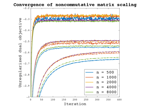
Figure 5.1: Convergence profile of noncommutative matrix scaling algorithm. The solid, dotted, and dot-dashed lines indicate $\beta=10$, $\beta=32$, and $\beta=100$, respectively, for a variety of problem sizes $n$. The convergence rate is observed empirically to be independent of $n$.

When $\beta$ is small, the regularization term might change the original unregularized SDP (5.2) significantly. Therefore we aim to quantify the impact of $\beta$ on the approximation ratio of the problem. It is known [9] that the GW relaxation achieves an approximation ratio of

$$\alpha=\frac{2}{\pi}\min_{\theta\in[0,\pi]}\frac{\theta}{1-\theta}\approx 0.878,$$

which is in fact the best possible approximation ratio if the unique games conjecture is true [12]. Note that a trivial approximation ratio of $1/2$ is always available (in expectation) by drawing each of the entries of $x$ independently randomly from the uniform distribution over $\{\pm 1\}$.

In Figure 5.2, we consider the effect of fixing $\beta$ and increasing the problem size in order to determine whether a constant approximation ratio is achieved as $n\rightarrow\infty$. We compute the approximation ratio as the ratio of the lower bound furnished as specified above to the expected lower bound (computed as an empirical average over 1000 samples) furnished as specified by steps 1-5 above. The optimization algorithm is run with batch size $N=8$ for 400 iterations in each case, except the case $\beta=100$ in which the optimization is run over 1000 iterations to ensure convergence. In the figure, we see that a constant nontrivial approximation ratio is maintained as $n$ becomes large. Moreover, the ratio is improved by enlarging $\beta$.

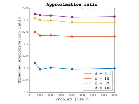
Figure 5.2: Approximation ratio of our algorithm as a function of problem size $n$ for various values of $\beta$. We observe empirically that a constant nontrivial approximation ratio is maintained as $n$ becomes large. The ratio is improved as $\beta$ increases.

5.2 Spectral embedding

The task of spectral embedding [20, 21] is to embed a graph into a Euclidean space in which the Euclidean distance is meaningful. Oftentimes, the graph is constructed from a point cloud in a preprocessing step via the selection of nearest neighbors or a procedure making use of a similarity kernel. After embedding, downstream tasks such as clustering can be significantly easier.

There are several approaches to spectral clustering given a graph, but a standard approach [21] is specified as follows. Given the adjacency matrix $A$ of the graph, let $D=\mathrm{diag}(A\mathbf{1}_{n})$ denote the diagonal matrix with diagonal entries given by the degrees of the corresponding graph vertices. Then a symmetric normalized graph Laplacian is constructed as

$$L=I-D^{-1/2}AD^{-1/2}.$$

If we desire a spectral embedding into $\mathbb{R}^{k}$, orthonormal eigenvectors corresponding to the $k$ lowest eigenvectors of $L$ are collected into the columns of $\Phi\in\mathbb{R}^{n\times k}$. The map $i\mapsto\Phi_{i,:}\in\mathbb{R}^{k}$ to the $i$-th row of matrix $\Phi$ then defines the spectral embedding map.

We rephrase the problem of determining $\Phi$ into the problem of determining $X=\Phi\Phi^{\top}$ via the SDP (2.7) in which we take $C=L$, and we introduce the binary von Neumann entropy with finite temperature $\beta$ as a regularization term.

5.2.1 Recovering the spectral embedding

Suppose we are given the regularized dual solution $\mu^{\star}$ and for simplicity denote $X=X(\mu^{\star})$ and $Y=Y(\mu^{\star})$. We now describe in principle how to recover an approximate spectral embedding from $\mu^{\star}$.

First create a random matrix $Z\in\mathbb{R}^{n\times\tilde{k}}$ consisting of entries drawn independently from the standard normal distribution. We denote the $i$-th column of $Z$ as $z^{(i)}$ and form

$$\Psi:=\frac{1}{\sqrt{\tilde{k}}}YZ\in\mathbb{R}^{n\times\tilde{k}}$$

with $i$-th column $\psi^{(i)}=\frac{1}{\sqrt{\tilde{k}}}Yz^{(i)}$. Note that forming $\Psi$ only requires matvecs by $Y=Y(\mu^{\star})=F_{\beta}^{1/2}(C-\mu^{\star}I)$, as in the optimization procedure itself.

We claim that the rows of $\Psi$ furnish an approximate spectral embedding in the sense that the Gram matrix of inner products $G:=\Psi\Psi^{\top}$ well approximates $X(\mu^{\star})=F_{\beta}(C-\mu I)$, which is itself a smoothed approximation to the spectral projector $\Phi\Phi^{\top}$ onto the lowest $k$ eigenvectors of $C$. Since pairwise inner products determine all the pairwise Euclidean distances, this implies that the embeddings $\Psi_{i,:}\in\mathbb{R}^{\tilde{k}}$ furnish an effective approximate solution to the original problem.

We want to justify that we can take $\tilde{k}=O(k\log n)$ in order to achieve a good approximation $\Psi\Psi^{\top}\approx X(\mu^{\star}).$ Then, assuming that the optimization furnishing $\mu^{\star}$ can be converged in $O(1)$ iterations, it would follow that approximate spectral embedding can be achieved in $O(kn\log n)$ time, which for large values of $k$ should outperform the usual $O(k^{2}n)$ scaling of determining $\Phi$ exactly.

Proposition 3.

Let $\delta\in(0,1/2]$, and suppose that $z^{(i)},i=1,\ldots,N$ are i.i.d. with entries that are themselves i.i.d. sub-Gaussian random variables with a constant sub-Gaussian parameter, mean zero, and unit variance. There exist constants $c,C>0$ such that if $\tilde{k}>c\log\left(\frac{n}{\delta}\right)$, then with probability at least $1-\delta$, the inequality

$$|G_{ij}-X_{ij}|\leq C\sqrt{\log\left(\frac{n}{\delta}\right)}\ \sqrt{\frac{X_{ii}X_{jj}}{\tilde{k}}}$$

holds for all $i,j=1,\ldots,n$. It follows that under the same conditions,

$$\frac{\|G-X\|_{\mathrm{F}}}{\|X\|_{\mathrm{F}}}\leq C\sqrt{\log\left(\frac{n}{\delta}\right)}\ \sqrt{\frac{k}{\tilde{k}}}\ \frac{\sqrt{k}}{\|X\|_{\mathrm{F}}}.$$

Remark 4.

Note that if $X=\Phi\Phi^{\top}$, then $\|X\|_{\mathrm{F}}=\sqrt{k}$. Even for finite $\beta$ where $X\approx\Phi\Phi^{\top}$ holds only approximately, for most reasonable models of the eigenvalues of the graph Laplacian $L$, we can expect that $\frac{\sqrt{k}}{\|X\|_{\mathrm{F}}}=O(1)$ for fixed $\beta$. Under this condition, to obtain an approximate spectral embedding of some fixed relative accuracy (in the sense of relative Frobenius norm error of the Gram matrix), we need only take $\tilde{k}=O(k\log n)$.

Proof.

Note that

$$G=\Psi\Psi^{\top}=\sum_{l=1}^{\tilde{k}}\psi^{(l)}\psi^{(l)\top}=\frac{1}{\tilde{k}}\sum_{l=1}^{\tilde{k}}Yz^{(l)}z^{(l)\top}Y.$$

Hence we can think of $G$ as an empirical expectation with $\mathbb{E}[G]=X$. In fact we can even think of it as a Hutchinson trace estimator for each entry $G_{ij}$ by rearranging

$$G_{ij}=e_{i}^{\top}Ge_{j}=\frac{1}{\tilde{k}}\sum_{l=1}^{\tilde{k}}z^{(l)\top}\left[Ye_{j}e_{i}^{\top}Y\right]z^{(l)}.$$

Hence $G_{ij}$ is a Hutchinson estimator for the trace $\mathrm{Tr}[Ye_{j}e_{i}^{\top}Y]$. Since

$$\|Ye_{j}e_{i}^{\top}Y\|_{\mathrm{F}}=\mathrm{Tr}\left[Ye_{j}e_{i}^{\top}YYe_{i}e_{j}^{\top}Y\right]=X_{ii}X_{jj},$$

we can again directly apply Lemma 2.1 of [17] to each Hutchinson estimator, $i,j=1,\ldots,n$, which, together with the union bound over the $n^{2}$ separate traces, implies the first statement of the proposition.

The second statement follows by recalling that $X=X(\mu^{\star})$ satisfies the constraint $\mathrm{Tr}[X]=k$, since it must be primal feasible. ∎

5.2.2 Experiments

We consider a random graph model with $n$ vertices in which $n$ is a multiple of $m$ and the subgraphs corresponding to the vertex subsets $\{1,\ldots,m\}$, $\{m+1,\ldots,2m\}$, …, and $\{n-m+1,\ldots,n\}$ are fully connected. In addition, every edge connecting two vertices appearing in distinct subsets is included with probability $1/n$. Thus the graph should be viewed as having $k=n/m$ clusters, which should be captured well by spectral embedding into $\mathbb{R}^{k}$.

As the approximation $X(\mu^{\star})=\Phi\Phi^{\top}$ can be well-understood in terms of the spectrum of $L$ and as the theory of recovering the spectral embedding is well-understood following Section 5.2.1, we focus in our experiments on the optimization, which is the point of more general interest for SDP with upper and lower semidefinite constraints.

Since the eigenvalues of the symmetric normalized graph Laplacian are bounded between $0$ and $2$ [5], following Section 3.3, we can take $R=2$ for our polynomial approximation of $F_{\beta}^{1/2}$. We insist on a sup norm error of at most $10^{-5}$ for our polynomial approximation over the interval $[-2,2]$.

In our experiments we take $m=10$, so $k=n/10$. Moreover, instead of computing each Newton step with high accuracy, we instead opt to take a small batch size $N=8$. Due to the large noise in the update, we can view our iterative optimization method as a stochastic process. At the $t$-th iteration, we compute a running average of the values of $\mu$ over the preceding $\left\lfloor t/2\right\rfloor$ iterations to obtain a convergent trajectory. In all experiments we run the procedure for $2000$ total iterations, and we plot the smoothed trajectories in Figure 5.3. At the end of the optimization, we verified using a Hutchinson estimator with $1000$ random vectors that the primal trace constraint $\mathrm{Tr}[X(\mu^{\star})]=k$ is satisfied to within relative error of 0.01 in all of our experiments. From Figure 5.3 we observe empirically that the convergence rate is independent of $n$.

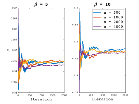
Figure 5.3: Smoothed optimization trajectory of $\mu$ for various problem sizes $n$. Left: $\beta=5$. Right: $\beta=10$. The convergence rate is observed to be empirically independent of $n$.

References

- [1] Awad H. Al-Mohy and Nicholas J. Higham. Computing the action of the matrix exponential, with an application to exponential integrators. SIAM Journal on Scientific Computing, 33(2):488–511, 2011.
- [2] C. Bekas, E. Kokiopoulou, and Y. Saad. An estimator for the diagonal of a matrix. Applied Numerical Mathematics, 57(11):1214–1229, 2007.
- [3] N. Boumal, B. Mishra, P.-A. Absil, and R. Sepulchre. Manopt, a Matlab toolbox for optimization on manifolds. Journal of Machine Learning Research, 15(42):1455–1459, 2014.
- [4] Samuel Burer and Renato D. C. Monteiro. A nonlinear programming algorithm for solving semidefinite programs via low-rank factorization. Mathematical Programming, 95(2):329–357, 2003.
- [5] Fan R. K. Chung. Spectral Graph Theory. American Mathematical Society, 1997.
- [6] M. Cuturi. Sinkhorn distances: Lightspeed computation of optimal transport. Advances in Neural Information Processing Systems, 26:2292–2300, 2013.
- [7] T. A Driscoll, N. Hale, and L. N. Trefethen. Chebfun Guide. Pafnuty Publications, 2014.
- [8] Paul Erdős and Alfréd Rényi. On random graphs. I. Publications Mathematicae, 6:290–297, 1959.
- [9] M. X. Goemans and D. P. Williamson. Improved approximation algorithms for maximum cut and satisfiability problems using semidefinite programming. J. ACM, 42:1115, 1995.
- [10] Sidney Golden. Lower bounds for the helmholtz function. Phys. Rev., 137:B1127–B1128, Feb 1965.
- [11] M.F. Hutchinson. A stochastic estimator of the trace of the influence matrix for laplacian smoothing splines. Communications in Statistics - Simulation and Computation, 19(2):433–450, 1990.
- [12] Subhash Khot, Guy Kindler, Elchanan Mossel, and Ryan O’Donnell. Optimal inapproximability results for max-cut and other 2-variable CSPs? SIAM Journal on Computing, 37(1):319–357, 2007.
- [13] A. V. Knyazev. Toward the optimal preconditioned eigensolver: Locally optimal block preconditioned conjugate gradient method. SIAM J. Sci. Comp., 23:517–541, 2001.
- [14] L. Lin and M. Lindsey. Variational embedding for quantum many-body problems. Commun. Pure Appl. Math., to appear.
- [15] Michael Lindsey. The quantum many-body problem: methods and analysis. PhD thesis, University of California, Berkeley, 2019.
- [16] Anant Mathur, Sarat Moka, and Zdravko Botev. Variance reduction for matrix computations with applications to gaussian processes. In Qianchuan Zhao and Li Xia, editors, Performance Evaluation Methodologies and Tools, pages 243–261, Cham, 2021. Springer International Publishing.
- [17] Raphael A. Meyer, Cameron Musco, Christopher Musco, and David P. Woodruff. Hutch++: Optimal Stochastic Trace Estimation, pages 142–155.
- [18] Dmitrii Pavlov. Logarithmically sparse symmetric matrices. arXiv:2301.10042.
- [19] Dmitrii Pavlov, Bernd Sturmfels, and Simon Telen. Gibbs manifolds. arXiv:2211.15490.
- [20] Alex Pothen, Horst D. Simon, and Kang-Pu Liou. Partitioning sparse matrices with eigenvectors of graphs. SIAM Journal on Matrix Analysis and Applications, 11(3):430–452, 1990.
- [21] Jianbo Shi and J. Malik. Normalized cuts and image segmentation. IEEE Transactions on Pattern Analysis and Machine Intelligence, 22(8):888–905, 2000.
- [22] C. J. Thompson. Inequality with applications in statistical mechanics. Journal of Mathematical Physics, 6:1812–1813, 1965.
- [23] Alp Yurtsever, Joel A. Tropp, Olivier Fercoq, Madeleine Udell, and Volkan Cevher. Scalable semidefinite programming. SIAM Journal on Mathematics of Data Science, 3(1):171–200, 2021.