The Winchcombe Fireball—that Lucky Survivor

Abstract

On February 28, 2021, a fireball dropped $\sim 0.6$ kg of recovered CM2 carbonaceous chondrite meteorites in South-West England near the town of Winchcombe. We reconstruct the fireball’s atmospheric trajectory, light curve, fragmentation behaviour, and pre-atmospheric orbit from optical records contributed by five networks. The progenitor meteoroid was three orders of magnitude less massive ($\sim 13$ kg) than any previously observed carbonaceous fall. The Winchcombe meteorite survived entry because it was exposed to a very low peak atmospheric dynamic pressure ($\sim 0.6$ MPa) due to a fortuitous combination of entry parameters, notably low velocity (13.9 km s^-1). A near-catastrophic fragmentation at $\sim 0.07$ MPa points to the body’s fragility. Low entry speeds which cause low peak dynamic pressures are likely necessary conditions for a small carbonaceous meteoroid to survive atmospheric entry, strongly constraining the radiant direction to the general antapex direction. Orbital integrations show that the meteoroid was injected into the near-Earth region $\sim 0.08$ Myr ago and it never had a perihelion distance smaller than $\sim 0.7$ AU, while other CM2 meteorites with known orbits approached the Sun closer ($\sim 0.5$ AU) and were heated to at least 100 K higher temperatures.

1 Introduction

On the 28th February 2021, at 21:54:16 UTC, a bright fireball lasting 8 seconds was observed above southern Wales, ending around Gloucester, UK (King et al., 2022). It was witnessed by over 1000 people and captured by many doorbell and dashboard cameras. It was also captured by 16 dedicated meteor/fireball cameras of the UK Fireball Alliance (UKFAll), making it a meteorite fall with one of the highest number of instrumental records to date.

The UKFAll consortium was established in 2018 as a collaboration between the five meteor camera networks in the UK, with an aim to streamline data sharing and meteorite recovery efforts (Daly et al., 2020). The precursory work that UKFAll had done prior to this event enabled the team to share data, establish an initial strewn field, and handle press inquiries, all within 12 hours of the fall. This streamlined process enabled the recovery of a portion of the 339 g main mass the morning following the fall. The meteorite was discovered as a rubble pile on a driveway in the town of Winchcombe, about 60 km south of Birmingham (King et al., 2022). The rest of the main mass was collected from this same site the next day, with another 283 g of fragments recovered from the surrounding area over the next week (Gattacceca et al., 2022). The meteorite was identified as a CM2 carbonaceous chondrite (Krot et al., 2014; Suttle et al., 2021); a rare type as only $\sim 4$% of meteorite falls globally are carbonaceous chondrites (Scott & Krot, 2014).

Instrumentally observing a meteorite fall enables the computation of its pre-atmospheric orbit (Ceplecha, 1961; Devillepoix et al., 2020). This can link the meteorite sample to a particular source region in the solar system (Granvik & Brown, 2018). Pairing an orbit with meteorite laboratory analyses enlightens our understanding of the composition of that particular region. Due to the presence of aqueous alteration (Bischoff, 1998), carbonaceous chondrites are known to have formed close to the snow line in the outer solar system (Krot et al., 2015). The exact mechanism of delivery of carbonaceous material into the asteroid belt is still a matter of discussion, but a migration event of the giant planets appears to be a necessary condition (Meech & Raymond, 2020; Vida et al., 2022).

Carbonaceous chondrites contain abundant water and organic matter (Trigo-Rodríguez et al., 2019; Matlovič et al., 2022). They are proposed as a significant source of Earth’s water and organic material so may be key to understanding the origins of life on Earth (Pizzarello et al., 2006; Marty, 2012; Alexander et al., 2012). Prior to the Winchcombe meteorite, only four carbonaceous chondrites have been linked to their pre-atmospheric orbit—Tagish Lake (Brown et al., 2000), Maribo (Haack et al., 2012), Sutter’s Mill (Jenniskens et al., 2012), and Flensburg (Borovička et al., 2021). However, none of them were well observed instrumentally from multiple stations and for most, trajectories were reconstructed from either casual images and videos or non-optical recordings.

Each of these events had a limited number of high-precision observations, especially from nearby dedicated cameras. Additionally, three out of four were daylight fireballs which makes calibration of video records more difficult, requiring the use of proxy objects as calibration points instead of stars (Borovička, 2014).

Winchcombe is the first carbonaceous chondrite fall which was recorded by multiple dedicated meteor/fireball cameras within 150 km of the fireball, and thus, observed with unprecedented detail. It was an evening event, providing both an opportunity for capturing high-precision optical recordings, as well as being widely witnessed—over 1000 eyewitness reports—resulting in much public interest.

In this paper, we perform a complete analysis of the fireball from the available optical records. In Section 2 we describe the observations and camera networks that observed the fireball. In Section 3 we discuss the trajectory and fragmentation modelling, continuing with the orbital analysis in Section 4. We compare the strewn field calculation with the locations of the meteorites found in Section 5. Finally, in Section 6 we put Winchcombe in context with previous orbital carbonaceous chondrites and discuss the relevance of this unique fall.

2 Data & Methods

Table 1: List of coordinates of UKFAll cameras that observed the Winchcombe fireball. The coordinates have been truncated to three decimal places due to privacy reasons, but the full trajectory solutions were produced using at least 5 decimal places ($\sim 1$ m accuracy). Astrometry/Photometry indicates whether the data from the camera was used for astrometric picks (A) or for photometry (P). The altitude is given in the mean sea level convention, not WGS84. F is the plate scale, and A err is the astrometric fit error.

Location	Network	Latitude (°)	Longitude (°)	Alt. (m)	Instrument	Used for	F (arcmin/px)	A err (arcmin)
Cardiff	SCAMP	51.486	-3.178	33	all-sky video	A + P	10.1	2.92
Cambridge	UKFN	52.165	0.039	8	all-sky photo	-	-	-
Chard	UKMON	50.878	-2.950	100	video	A	5.8	1.25
Chelmsford	NEMETODE	51.745	0.494	45	video	-	-	-
Clanfield	UKMON	50.939	-1.020	158	video	-	-	-
Honiton	SCAMP	50.802	-3.184	119	all-sky video	A + P	10.1	3.42
Hullavington	GMN	51.535	-2.149	103	video	A	3.8	0.83
Lincoln	UKFN	53.222	-0.464	16	all-sky photo	A	2.0	0.64
Loughborough	NEMETODE	52.751	-1.213	73	video	-	-	-
Manchester	SCAMP	53.474	-2.234	69	all-sky video	P	-	-
Ringwood	GMN	50.858	-1.778	24	video	A	3.8	1.32
Tackley	GMN	51.883	-1.306	80	video	-	-	-
Welwyn	UKFN	51.268	-0.394	78	all-sky photo	A	2.0	1.04
Wilcot	UKMON	51.352	-1.802	133	video	P	-	-

The details of cameras that observed the fireball are given in Table 1. All networks which contributed optical observations are part of the UK Fireball Alliance (Daly et al., 2020). Figure 1 shows the image of the fireball from several cameras.

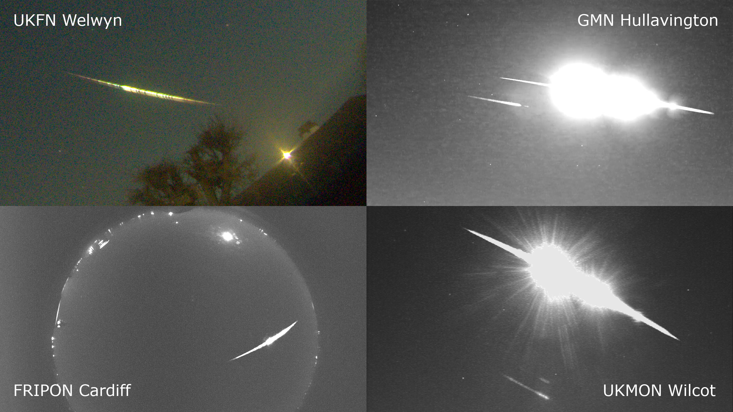
Figure 1: The Winchcombe fireball as seen from Welwyn (upper left), Hullavington (upper right), Cardiff (bottom left), and Wilcot (bottom right). The Hullavington and Wilcot images show a reflection parallel to the fireball. The fireball is moving from left to right in all images.

After the fall, all astrometry and photometry measurements produced by individual networks were mutually exchanged through the Global Fireball Exchange format (Rowe et al., 2020). Standard specifications are documented at https://github.com/UKFAll/standard, and the full final measurements are given in Supplementary Materials in this format.

Although each network employs its own reduction software suite for day-to-day operations, all astrometric and photometric data used for the analysis presented in this work have been re-measured following the methods of Vida et al. (2021b). In this section, we provide a brief description of each camera network.

2.1 SCAMP/FRIPON

SCAMP, the System for the Capture of Asteroid and Meteorite Paths, is the UK arm of the French Fireball Recovery and InterPlanetary Observation Network (FRIPON) that extends over Europe (Colas et al., 2020). This network uses cameras with an all-sky lens to capture high-resolution video recordings (30 frames per second) of fireballs (Colas et al., 2015). There are currently 7 cameras in the UK network, with the aim to have 72 cameras in total to provide full coverage of the UK and Ireland.

2.2 UKFN/GFO

UKFN, the UK Fireball Network is the UK arm of the Global Fireball Observatory (GFO) collaboration (Devillepoix et al., 2020). This network uses all-sky cameras based on the DSLR system developed by the Desert Fireball Network (DFN) in Australia (Howie et al., 2017a). These cameras capture a 27 s long-exposure photograph every 30 seconds. Absolute timing along the fireball track is encoded using a liquid crystal shutter and the de Bruijn method of Howie et al. (2017b). The cameras require a spacing of $<$200 km for accurate fireball detection and observation (Devillepoix et al., 2019); there are currently 6 cameras deployed in the UK, with plans to expand the network to a total of 11 cameras in the British Isles.

2.3 GMN

The Global Meteor Network (GMN) operates over 700 video meteor stations in 38 countries (Vida et al., 2021b). The stations use low-cost consumer-grade IMX291 and IMX307 CMOS sensors paired with wide-field lenses (most commonly $88^{\circ}\times 48^{\circ}$). All cameras are operated at 25 frames per second. 3.6 mm and 6 mm f/0.95 lenses are most commonly used, giving a similar field of view and sensitivity to a human observer (limiting magnitude $+6.0^{\mathrm{M}}\pm 0.5^{\mathrm{M}}$. The cameras are connected to Raspberry Pi single-board computers which run open-source software (Vida et al., 2016, 2018). Currently (circa. mid-2022), the GMN operates around 220 cameras in the UK.

2.4 UKMON

UKMON, the UK Meteor Network, is a group of amateur astronomers who use commercial CCTV video cameras for meteor monitoring (Campbell-Burns & Kacerek, 2014). The network’s main focus are fainter meteors and meteor showers, however the cameras also detect fireballs. The UKMON mainly uses GMN camera systems but also operates several older analog Watec cameras. UKMON currently has over 200 cameras in the UK, but at the time of the Winchcombe fall only around 30 cameras were installed.

2.5 NEMETODE

NEMETODE, the Network for Meteor Triangulation and Orbit Determination, is an amateur group with a network of analog and digital cameras to monitor the night sky for meteors and meteor showers, mostly based on UFOCapture software (Stewart et al., 2013). Currently, NEMETODE has over 40 stations, generally with multiple cameras at each station, with significant coverage of much of Northern England and Ireland.

2.6 Other data

Other observational data of the Winchcombe fall were collected along with the optical data described above. However, as they did not inform the astrometric and entry modelling of the Winchcombe fall we only briefly summarise them below:

• A low-resolution visible spectrum was captured by two cameras (NEMETODE and UKMON).

• Some infrasound signals were detected by sensors from the Raspberry Shake & Boom network , however no useful measurements could be made due to data timestamping issues.

• No seismic signals were detected by any seismographs within 200 km.

3 Trajectory

In this section, we describe the details of the trajectory, discuss the data reduction procedure and calibration quality, and present the results of fireball ablation modelling.

3.1 Astrometry and photometry

All optical data sets were manually calibrated and reduced using the SkyFit2 software (Vida et al., 2021b). Both the all-sky and narrow-field data were calibrated using the radial distortion model with odd terms up to the seventh order ($r,r^{3},r^{5},r^{7}$), taking atmospheric refraction and lens anisotropy into account. All calibrations showed only random errors with no systematic trends. Table 1 summarises the cameras used in the solution, together with the plate scales and the average astrometric fit errors, which were on the order of a few arc minutes for all systems. Of the total 16 cameras which observed the fireball, only seven were used in the final trajectory solution. Others were less optimal due to large distance, bad geometry, CCD blooming, or frame drops. We note that these data would also be useful if the seven picked stations did not offer the best view of the fireball.

The unsaturated light curve was exclusively measured on SCAMP video data for magnitudes fainter than $-8^{\mathrm{M}}$, at which point the cameras saturated (Cardiff, Honiton, and Manchester stations). All other cameras were either already saturated or observed the fireball through thin clouds which would degrade the quality of photometry measurements. Fortuitously, during the time of SCAMP camera saturation, the analogue CCD camera video from Wilcot showed an unsaturated lens reflection which was used to measure the brightest portion of the fireball. Independent absolute calibration of the reflection could not be done, the measurements yielding only an instrumental magnitude estimate. However, there were several common points with the unsaturated SCAMP portion of the light curve which were used to scale the instrumental magnitude of the reflection, allowing the full light curve to be reconstructed to a high degree of accuracy. Fig. 6 shows the measured light curve.

3.2 Atmospheric trajectory

The nominal trajectory and orbital solution were calculated using the method of Vida et al. (2020). The uncertainties were computed by adding Gaussian noise that is two times larger than the measured random fit errors, as per Vida et al. (2020), and re-fitting the trajectory solution. The trajectory details are given in Table 2. Figure 2 shows the fireball trajectory in relation to the seven stations. All selected stations are within 200 km of the fireball, and the Hullavington station was only 50 km away, allowing it to capture the details of fragmentation and track the final fragments just before the dark flight began. Despite most stations being south of the fireball, the observation geometry was favourable — the maximum convergence angle of 89^∘ was between the Cardiff and Welwyn stations.

Table 2: Fireball trajectory parameters with associated $1\sigma$ uncertainties. All values are given in the Earth-fixed system. The values of initial and final azimuth and altitude differ because the trajectory of the fireball is considered to be a straight line in the Earth-Centred Inertial (ECI) coordinate system, and are recomputed to ground-fixed values to be compatible with previous publications. The final azimuth and altitude do not take the deviating fragment into account.

	Beginning	End
Time	21:54:15.88	21:54:24.12
Latitude (+N)	51.870970∘	51.940114∘
	$\pm$15.3 m	$\pm$16.2 m
Longitude (+E)	-3.109378∘	-2.096335∘
	$\pm$8.8 m	$\pm$5.6 m
Height (km)	90.599	27.554
	$\pm$0.020	$\pm$0.015
Velocity (km s-1)	13.86	$\sim 3$
	$\pm 0.01$	-
Azimuth	263.342∘	263.906∘
	0.046∘	-
Altitude	41.919∘	41.530∘
	0.029∘	-

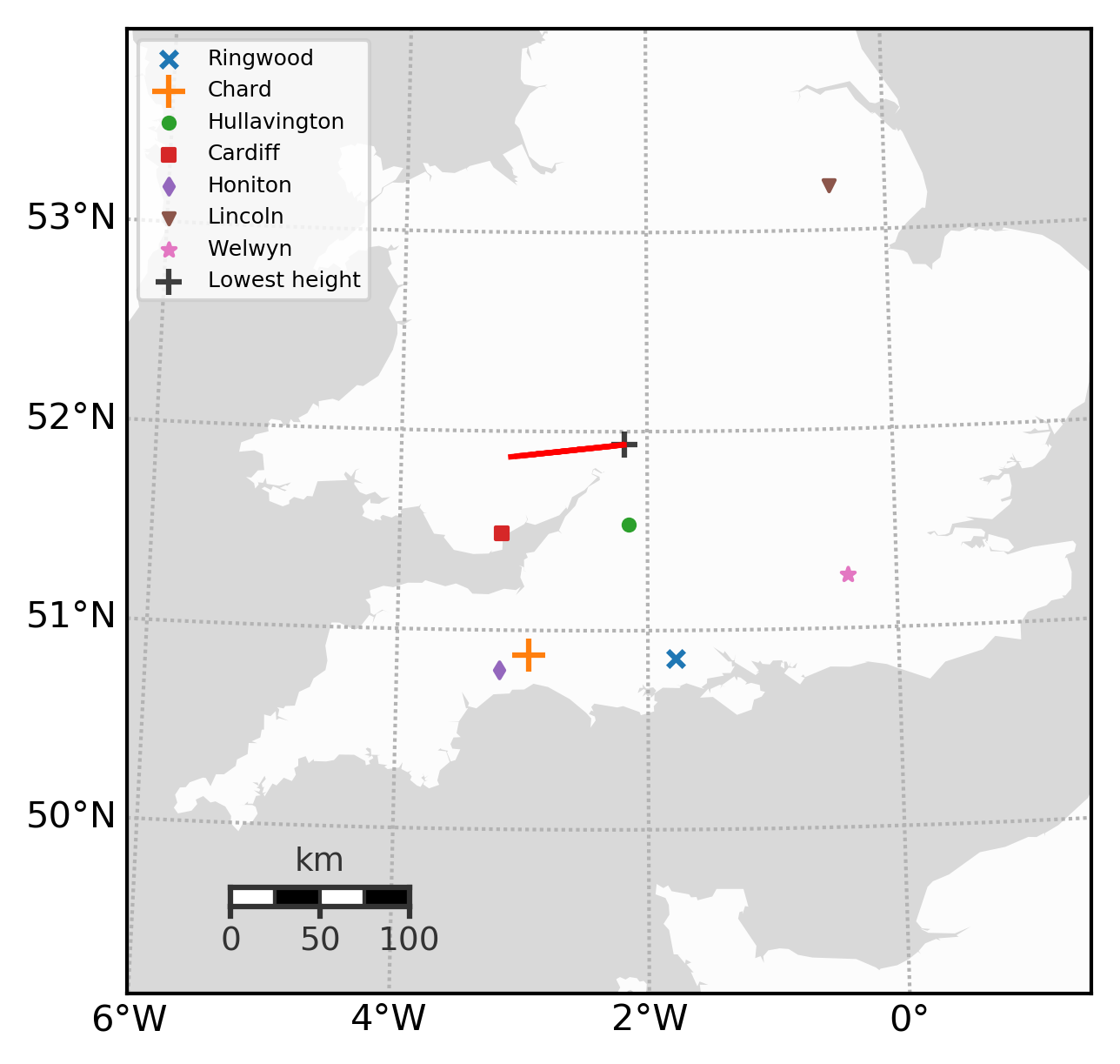
Figure 2: The Winchcombe fireball trajectory (red line) and locations of cameras used for astrometric measurements.

Figure 3 shows the trajectory fit residuals from a straight line. The trajectory fit residuals were all below 100 m across the observed span of almost 100 km. Following Vida et al. (2020), the initial velocity was computed as the average velocity up to the time when deceleration became statistically significant. This is achieved by progressively including more points from the beginning of the trajectory until the end in a linear time vs. distance fit, and choosing the solution with the smallest standard deviation. The fireball was first observed at the height of 90.6 km moving at a velocity of 13.86 km s^-1, and it was last observed at 27.6 km decelerating below the ablation limit at 3 km s^-1.

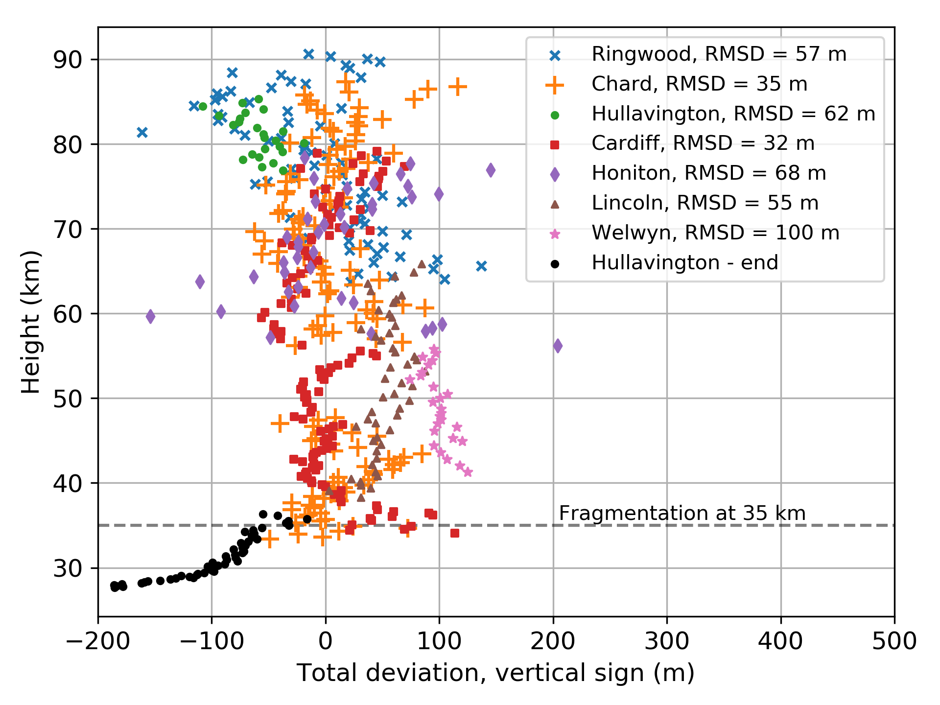
Figure 3: Total trajectory fit residuals versus height (the sign of the deviation is taken from the vertical direction). RMSD stands for root-mean-square deviation. The measurements from Hullavington were only done at the beginning and the end, as the fireball was too bright in the middle of the flight for accurate astrometric picks.

The Winchcombe meteoroid experienced several major fragmentation, dramatically increasing the observed fireball brightness and deceleration. The trajectory followed a straight line up until the final fragmentation at a height of 35 km. A sudden change in the direction of fragments was observed afterwards. The final portion of the trajectory which showed the deviation was only observed from the Hullavington station due to its closeness to the fireball and higher sensitivity. This final portion was either outside of the fields of view of other cameras, or they were not sensitive enough to observe it. The observed deviation was not due to calibration issues—the total observed deviation from a straight-line trajectory was 12 arc minutes, and the astrometry fit accuracy around the end of the fireball was 0.83 arc minutes. The apparent cross-track velocity of the fragment relative to a straight line was $\sim 100$ m s^-1; however, this represents a lower limit as the orientation of the plane of fragmentation cannot be measured from a single-station observation. Only the part of the trajectory above 35 km was used for orbit estimation, to avoid any influence of the deviating fragment on the radiant.

3.3 Final mass estimation

This final fragmentation produced four discrete fragments (Figure 4) that could be individually tracked until they dimmed below magnitude $+2^{\mathrm{M}}$. These measurements allowed an accurate estimation of the dynamic mass of the largest fragment (Figure 5). Following a classical approach (McCrosky et al., 1971), a line was fit on time vs. velocity measurements near the fireball’s end to obtain an estimate of the velocity and the deceleration. The dynamic mass $m_{dyn}$ is computed as:

$$m_{dyn}=\frac{1}{\rho_{m}^{2}}\left(\frac{\Gamma A\rho_{a}v^{2}}{\dot{v}}\right)^{3}\,,$$ (1)

where $\rho_{m}$ is the meteoroid bulk density, $\Gamma$ is the drag factor, $A$ is the shape factor, and $\rho_{a}$ is the atmospheric mass density at the point where the velocity $v$ and deceleration $\dot{v}$ are measured.

In this method, the underlying assumption is that the mass loss is no longer the dominant driver of energy loss and that the fit can be fully described by the single-body drag equation. A bulk density of $\rho_{m}=$2100 kg m^-3 was used, informed by the atmospheric ablation characteristics which indicate a carbonaceous body. This is consistent with the density of the recovered meteorites from micro-X-ray computed tomography ($\sim$2090 kg m^-3 King et al. 2022). The product $\Gamma A$ can be treated as a free parameter, and has previously been found empirically to fall in the 0.5–1.0 range near the end of fireballs, representing spherical to cylindrical shapes (Boroviĉka & Kalenda, 2003; Borovička et al., 2015; Gritsevich et al., 2014).

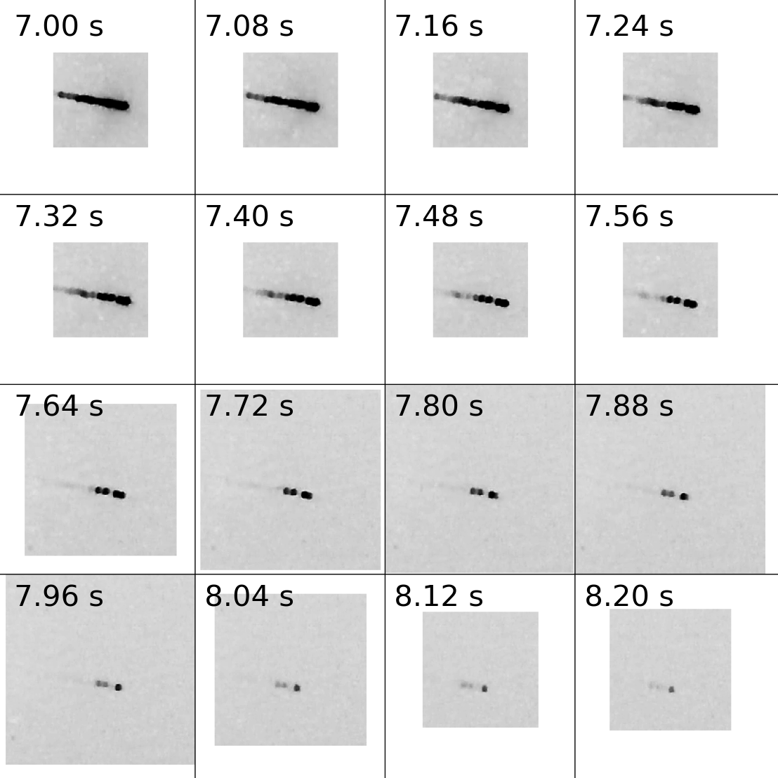
Figure 4: Colour-inverted mosaic of the last moments (every second frame) observed from Hullavington. Four discrete fragments can be seen at the end.

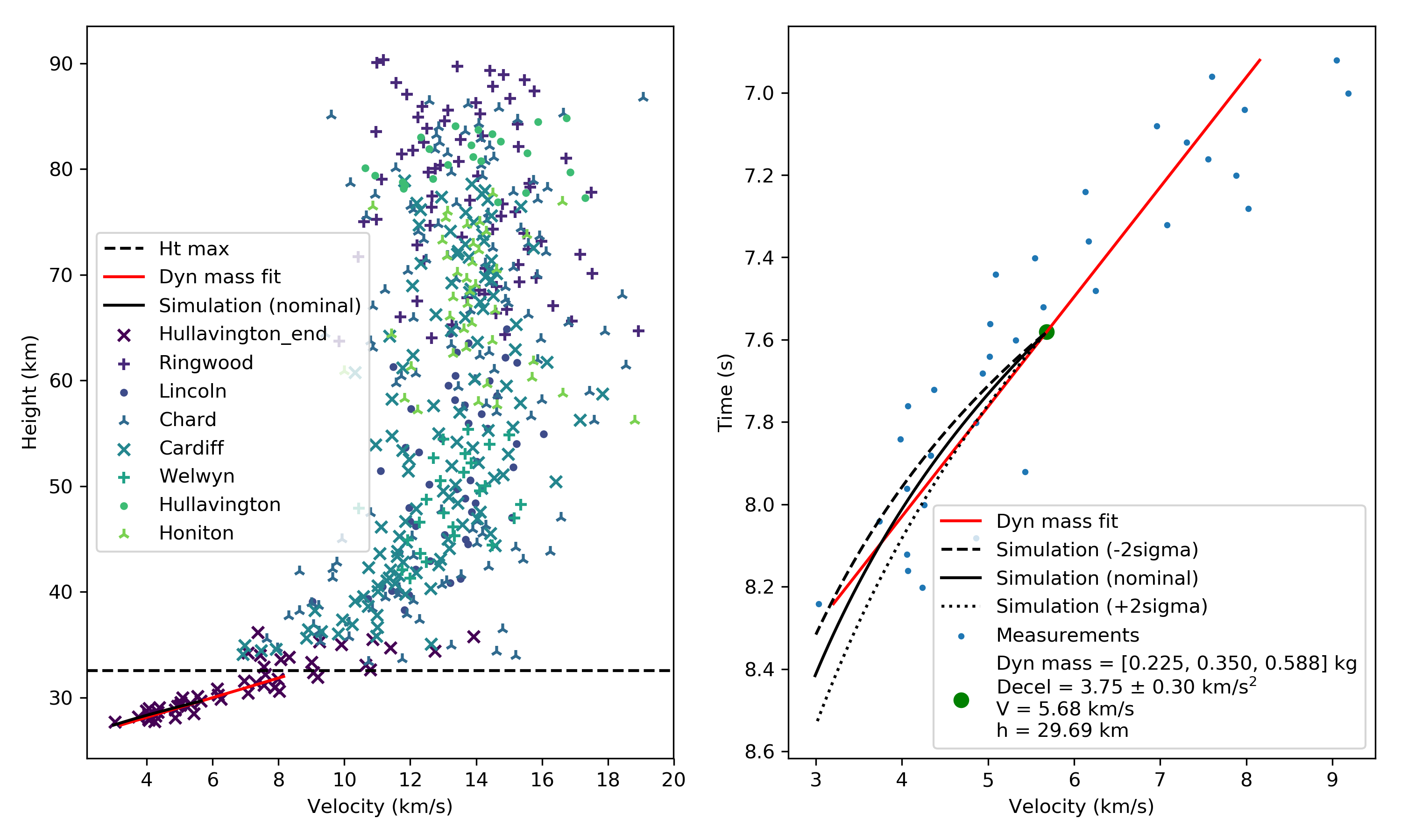
Figure 5: Left: Observed point-to-point velocities, and the dynamic mass fit (red line) done using final velocity measurements below the dashed line. Right: A section of velocity measurements at the end of the fireball (blue dots) used for the dynamic mass fit (red line). The mass was estimated in the middle (green dot). Black lines indicate the nominal simulation (solid) and the $2\sigma$ variations (dashed and dotted).

To constrain the mass by adjusting the $\Gamma A$ factor, and to compute the final location of the fragments prior to dark flight, we introduce a novel method. We perform a forward integration of single-body ablation equations (Ceplecha et al., 1998) starting at the point where the dynamic mass is estimated. The equations are integrated until the velocity falls below 3 km s^-1, i.e. the ablation limit. An intrinsic ablation coefficient of $\sigma=0.005$ kg MJ^-1 is used (Ceplecha et al., 1998). $\Gamma A$ factor is adjusted until the simulated velocity matches the observed velocity at the end. The final geographical coordinates and height above ground are computed at the cessation of ablation and are used for dark flight modelling. The azimuth and elevation of the trajectory with respect to the ground at this endpoint are computed taking the drop due to gravity and the curvature of the Earth into account.

$\Gamma A=0.55$ was found to best fit the observations. A range of masses between 0.225 and 0.588 kg was measured (95% confidence interval) for the main fragment, with 0.350 kg being the nominal value. The dynamic mass was estimated at the height of 29.69 km and at the velocity of 5.68 km s^-1, at which a deceleration of $3.75\pm 0.30$ km s^-2 was measured. The NRLMSISE-00 model (Picone et al., 2002) was used to obtain the atmospheric mass density. After integrating the ablation equations, only a further 5% of mass was lost (the final nominal value for the main fragment was 0.330 kg). This nominal estimate for the lead fragment is consistent with the largest sample recovered which has a mass of 0.319 kg. The dynamic mass estimates for the smaller fragments are between 50 and 100 g, which is also consistent with the other recovered samples (King et al., 2022).

3.4 Dynamics and Fragmentation Modelling

The dynamics, light curve, and fragmentation behaviour were modelled using the Borovička et al. (2013) semi-empirical ablation model. The manual modelling procedure described in detail in Borovička et al. (2020) was followed. The luminous efficiency model used was from the same paper. Of the many semi-analytical approaches developed to model meteoroid trajectories and fragmentation processes in our atmosphere (e.g. Johnston et al., 2018; Wheeler et al., 2017), this method gives us the highest fidelity and enables direct modelling of each observed feature and fragment individually.

In summary, the initial meteoroid is modelled as a classical single body that fragments at manually determined points. Physical parameters of the initial meteoroid and individual fragments are also manually estimated. All generated fragments are considered single bodies. The fragmentation points are informed by brightness increases in the light curve (i.e. flares) and increases in the observed deceleration. Most fragmentations were modelled as a release of an eroding fragment (see Borovička et al., 2015, for more details) which is a body that rapidly erodes by the release of mm-sized grains. The grain masses are distributed according to a power law (differential mass index of $s=2.0$ is assumed) within a given range of masses. The amount of erosion is regulated by the erosion coefficient $\eta$, which determines how much mass is eroded from the fragment per unit of kinetic energy loss.

An excellent fit to the data was obtained, within observational uncertainty (Figure 6). The only significant discrepancy between the model and observations is at the beginning of the fireball above $\sim 60$ km. For this portion, the fit of the model to the light curve could not be improved, even with an unphysical and extremely low ablation coefficient of $\sigma=0.0001$ kg MJ^-1 ($50\times$ lower than the intrinsic $\sigma$ of ordinary chondrites). This suggests a significant influence of preheating of carbonaceous material, as was similarly noticed for ordinary chondrites (Spurnỳ et al., 2020). The model indicates that the mass loss was not important in this initial stage, meaning the light production was purely caused by the drag component. This discrepancy calls for a revision of luminous efficiency models or a separation of models into mass loss and drag components with different values. For example, Borovička et al. (2011) have measured a luminous efficiency of the drag component of the Hayabusa capsule re-entry, as its ablation shield prevented any significant mass loss. The capsule entered the atmosphere at 12 km s^-1, a similar speed to Winchcombe, and its observed luminous efficiency was 1.3%. The luminous efficiency in our model was $\sim 5\%$, which can explain the observed discrepancy. Nevertheless, the initial portion of the light curve does not play a significant role in deriving physical properties nor fragmentation behaviour and does not affect the conclusions below which stand for the given model assumptions.

The inverted physical properties of the fireball are given in Table 3 and the fragmentation behaviour is given in Table 4. We note that error estimation remains a challenge with this empirical method, and this might not be a unique solution, thus concrete error estimates are hard to give (Vida et al., 2022). Nevertheless, the data is accurate enough to constrain the model bulk density to $\pm 10$ kg m^-3 while keeping all other parameters fixed. Progressive fragmentation was not modelled, so it was assumed that the released fragments do not have an intrinsic ablation coefficient $\sigma=0.005$ kg MJ^-1 of ordinary chondrites, but an apparent ablation coefficient appropriate for C-type meteoroids $\sigma=0.04$ kg MJ^-1 (Ceplecha et al., 1998).

Table 3: Modelled physical properties of the fireball.

Description		Value
Initial mass (kg)	$m_{0}$	12.5
Initial speed at 180 km (km s-1)	$v_{0}$	13.86
Zenith angle	$Z_{c}$	$48.08^{\circ}$
Bulk density (kg m-3)	$\rho$	2100
Grain density (kg m-3)	$\rho_{g}$	3000
Ablation coefficient (kg MJ-1)	$\sigma$	0.005
(above 66 km)	$\sigma$	$<$0.0001
Shape factor (sphere)	$A$	1.21
Drag factor	$\Gamma$	0.8
(above 66 km)	$\Gamma$	1.0
(below 35.1 km)	$\Gamma$	0.55

Table 4: Modelled fragmentation behaviour. The fragment mass percentage in the table is reference to the mass of the main fragment at the moment of ejection. The mass distribution index for all grains was $s=2.0$. The values of the dynamic pressure are computed using the drag factor $\Gamma=1.0$.

Timea	Height	Velocity	Dyn pres	Main $m$	Fragment	$m$	$m$	Erosion coeff	Grain $m$	Meteorites
(s)	(km)	(km s-1)	(MPa)	(kg)		(%)	(kg)	(kg MJ-1)	range (kg)	Mass (kg)
2.71	65.30	13.80	0.025	12.50	EF	0.2	0.025	1.50	$10^{-9}-10^{-8}$	-
3.06	62.00	13.78	0.040	12.45	EF	1.0	0.124	1.00	$10^{-9}-10^{-8}$	-
3.39	59.00	13.73	0.059	12.29	EF	1.5	0.184	1.00	$10^{-9}-10^{-8}$	-
3.68	56.25	13.68	0.083	12.06	EF	36.0	4.341	0.10	$10^{-4}-10^{-3}$	-
3.69	56.20	13.68	0.084	7.72	EF	46.0	3.550	0.80	$10^{-5}-10^{-3}$	-
4.58	48.00	13.22	0.214	4.04	EF	20.0	0.808	0.05	$10^{-4}-10^{-3}$	-
4.81	46.00	13.00	0.265	3.19	EF	30.0	0.956	0.05	$10^{-4}-10^{-3}$	-
4.98	44.50	12.78	0.307	2.20	EF	30.0	0.660	0.10	$10^{-6}-10^{-4}$	-
5.42	40.80	11.94	0.428	1.46	EF	37.0	0.541	0.05	$10^{-4}-10^{-3}$	$10^{-3}$
6.19	35.10	9.45	0.584	0.81	D	28.0	0.226	-	$10^{-5}-10^{-3}$
6.23	34.90	9.35	0.591	0.58	$3\times$ F	25.0	0.144	-	-	$3\times 0.12$
Endb	25.31	-	-	-	-	-	-	-	-	0.35
a Seconds after 2021-02-28 21:54:15.9 UTC.
b Final mass of the main fragment at the end of ablation.
EF = New eroding fragment; D = Dust ejection; F = Single-body fragment.

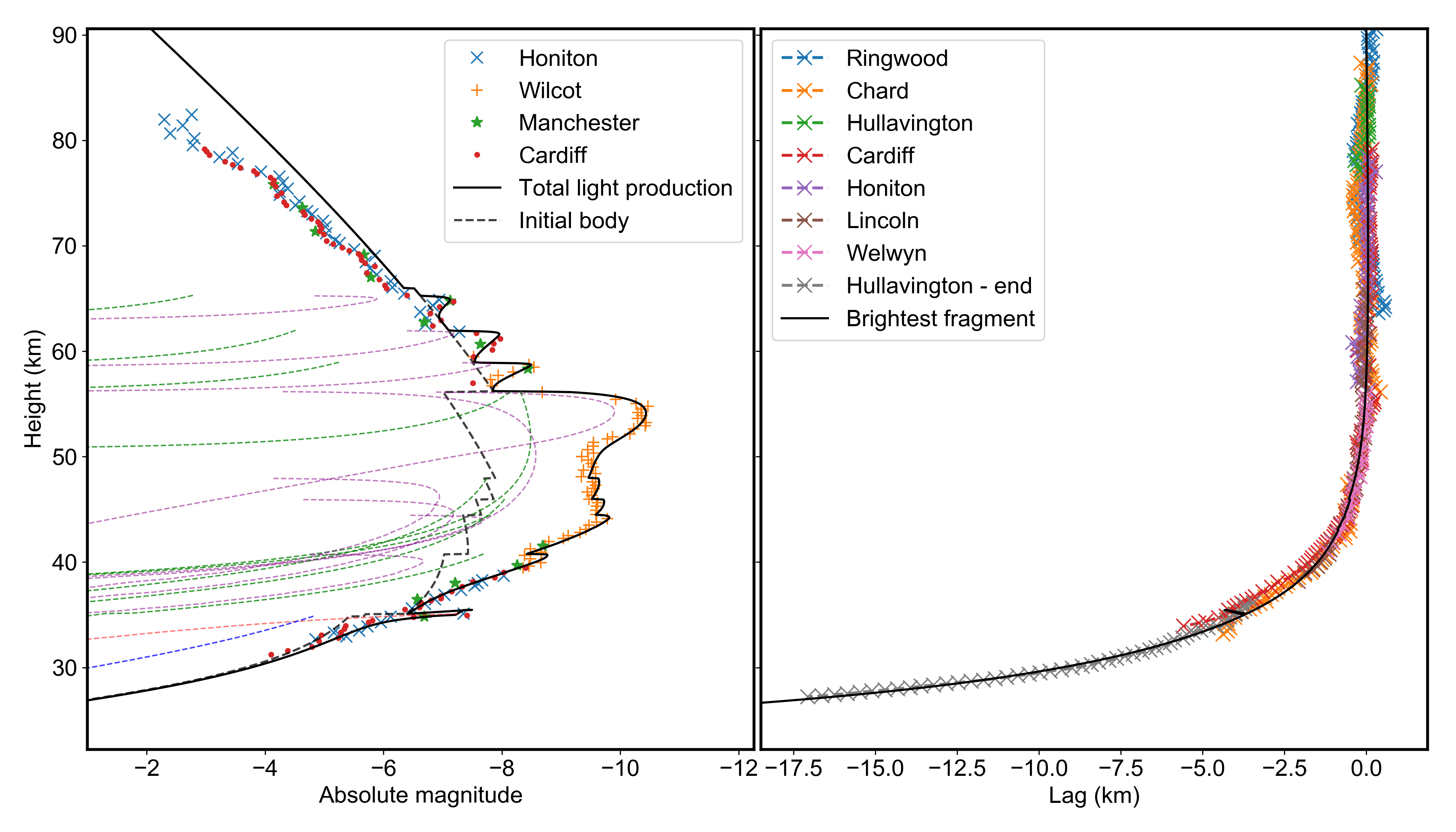
Figure 6: Fit of the ablation model (black line) to the observed light curve (left) and the lag (right) for the Winchcombe fireball. The lag is the distance a decelerating meteoroid falls behind a hypothetical non-decelerating meteoroid moving at the initially observed velocity (Vida et al., 2021a). Inferred contributions to the total light production of individual fragments are given in dashed lines; black for the magnitude of the main body, green for eroding fragments, purple for grains released by erosion, blue for single-body fragments, and orange for dust released directly from the main body.

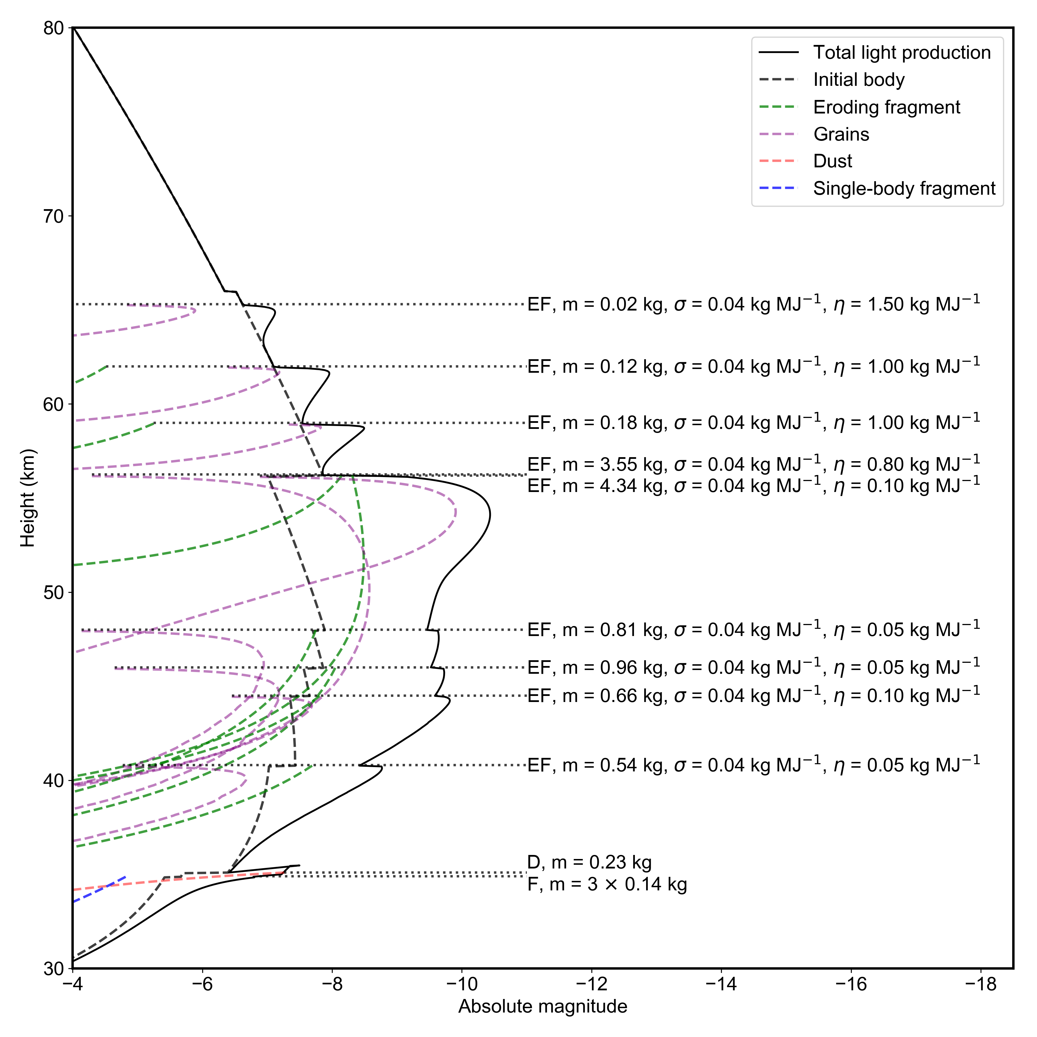
Figure 7: Details of individual fragmentation events. The fragmentation points, the type of fragmentation, total fragment mass, fragment ablation and erosion coefficients are shown.

Figure 7 shows the details of the modelled fragmentation events. Starting with an initial mass of 12.53 kg, the meteoroid only experienced minor fragmentation (a loss of a few percent of mass) above 60 km of height, at dynamic pressures $P_{\mathrm{dyn}}\lesssim 0.06$ MPa (Figure 8; $P_{\mathrm{dyn}}=\Gamma\rho_{a}v^{2}$, where $\rho_{a}$ is the atmospheric mass density at a given height and $v$ is the meteoroid speed at that height). However, the rapid mass loss occurred between $0.08$–$0.1$ MPa when over 80% of mass was lost into two eroding fragments. The fireball continued to lose 20-30% of instantaneous mass ($\sim 0.5$ kg each) in each of the five subsequent fragmentations between $0.1$–$0.5$ MPa. Due to rapid deceleration, the rise in the dynamic pressure slowed and the fireball only reached a peak pressure of $0.6$ MPa at the height of 35 km. At this point of peak pressure, a final fragmentation with a sharp flare was observed which could only be explained by a sudden release of mm-sized dust.

Direct observations of the fragment train from the Hullavington station (Figure 4) showed that the final fragmentation event at the height of 35 km produced four distinct fragments. We reproduce the observed fragment mass distribution by assuming the final fragmentation produces three $\sim 100$ g fragments. Even smaller fragments have also been observed in the video, but there is no practical way to directly measure their size. We note that 10 fragments total have been recovered (Russell et al., 2022), which is at odds with the four final fragments observed in the video. However, further fragmentation during the dark flight is a known phenomenon that might have been significant for this fragile body (Boroviĉka & Kalenda, 2003; Spurnỳ et al., 2020), and some may even have been released higher up and obscured by the wake.

The fragmentation of Winchcombe occurred at dynamic pressures consistent with previously observed carbonaceous chondrite falls (Figure 8), which have also all shown fragmentation in the $0.1$–$0.5$ MPa range (Borovička et al., 2019, 2021). This is in stark contrast to ordinary chondrites which have two distinct phases of fragmentation, the first between 0.04–0.12 MPa and the second between 0.5–5 MPa Borovička et al. (2020).

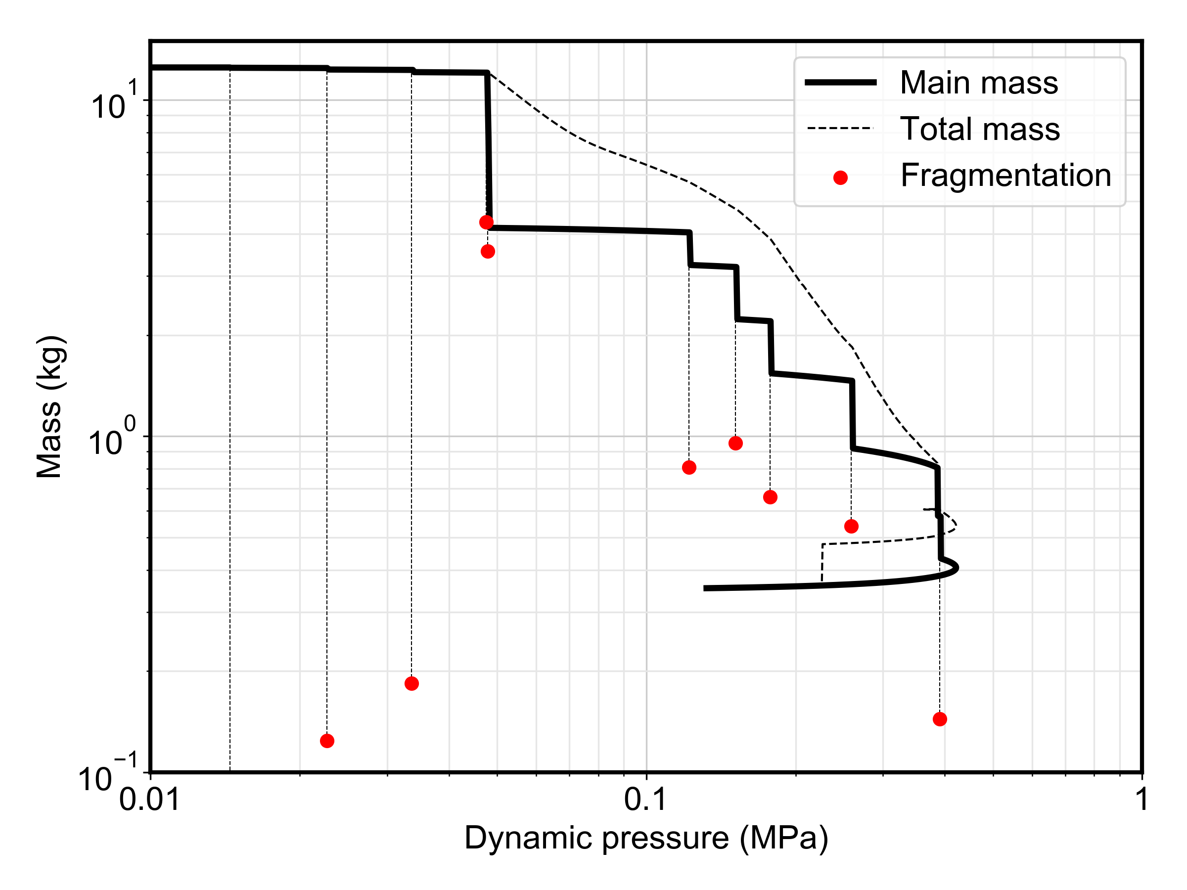
Figure 8: Mass of the main fragment (solid line) and the total mass (dashed line) versus the dynamic pressure. Individual fragmentation points and the total fragment masses are marked in red circles. The first fragmentation ($m=0.02$ kg) is outside the plot for presentation purposes.

4 Orbital analysis

4.1 Radiant and pre-encounter orbit

The pre-encounter orbit was calculated from a trajectory that excluded all measurements below 35 km (Sec. 3), due to the fragment deviation below that altitude. Orbital elements are given in Table 5. Winchcombe’s orbit is well within the main belt (not evolved). The semi-major axis (2.5855 AU) places it between the 3:1 (2.5 AU) and the 5:2 (2.82 AU) mean-motion resonances with Jupiter, and points to these as probable mechanisms for delivering Winchcombe to near-Earth space. Although Winchcombe shares a mid-belt semi-major axis with two other CM2 meteorites (Sutter’s Mill (Jenniskens et al., 2012) and Maribo (Borovička et al., 2019)), its Tisserand parameter with respect to Jupiter (T_J = 3.12) places it on the asteroid side (T${}_{J}>$3), contrary to the other two. The dynamical evolution of these objects can sometimes obfuscate their true origins Shober et al. (2021).

Table 5: Pre-encounter orbital parameters expressed in the heliocentric ecliptic frame (J2000) and associated $1\sigma$ formal uncertainties.

	Unit	Value	$1\sigma$	95% Confidence Interval
				Lower	Upper
Semi-major axis	AU	2.5855	$\pm 0.0077$	2.5686	2.5980
Eccentricity		0.6183	$\pm 0.0011$	0.6158	0.6201
Inclination	°	0.460	$\pm 0.014$	0.440	0.490
Argument of periapsis	°	351.798	$\pm 0.018$	351.759	351.824
Longitude ascending node	°	160.1955	$\pm 0.0014$	160.1933	160.1985
Perihelion	AU	0.986839	$\pm 0.000012$	0.986814	0.986861
Aphelion	AU	4.184	$\pm 0.015$	4.150	4.209
Tisserand’s parameter		3.1207	$\pm 0.0056$	3.1117	3.1331
Last perihelion	days	2021 Feb 22.446	$\pm 0.015$	22.413	22.469
Geocentric Right Ascension	°	56.638	$\pm 0.017$	56.604	56.671
Geocentric Declination	°	17.713	$\pm 0.069$	17.555	17.816
Geocentric velocity	m s-1	8123	$\pm 13$	8093	8143

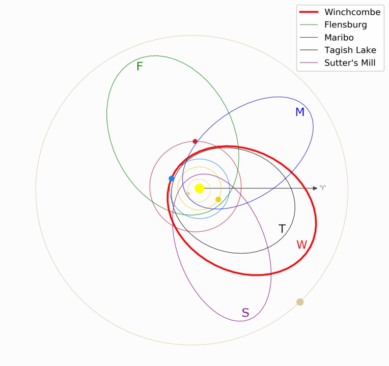
Figure 9: Ecliptic projection representing the pre-encounter orbit of the Winchcombe meteoroid, in context with other carbonaceous orbital meteorites. Inclination to the ecliptic for Winchcombe is 0.46°.

4.2 Orbital history

To gain insight into the recent dynamical past of the meteoroid before it crossed the Earth’s path, we use backward integrations of the orbit following the method used by Shober et al. (2021). 1000 orbital clones of the meteoroid are created based on the uncertainties (Table 2) and then integrated backwards using the Rebound IAS15 adaptive time step integrator (Rein & Spiegel, 2015) with the Sun, 8 planets, and the Moon as active bodies. The state vector of the test particles is recorded every 1000 years, both in barycentric coordinates and as osculating ecliptic orbital elements. Backward integrations ended at 3 million years in the past, way past the time for which meaningful dynamical insights into the meteoroid’s history can be gained. Because the meteoroid was affected by Earth, Mars, and Jupiter in the recent past, the dynamical system is very rapidly chaotic. In post-analysis, we record at what time each meteoroid clone entered near-Earth space (perihelion distance $<1.3$ AU). This gives us a median near-Earth entry of $\sim$0.08 Myr in the past, with 50% of particles entering between 0.035 and 0.24 Myr ago. In comparison, measured cosmic-ray exposure ages for Winchcombe are $\sim$0.3 Myr for ²¹Ne and 0.27 $\pm$ 0.08 Myr for ²⁶Al (King et al., 2022). This indicates that the ejection of the Winchcombe meteoroid from a larger parent asteroid (start of exposure to cosmic rays), and its orbital migration from the main belt to near-Earth space were either contemporaneous events or the ejection happened while the parent body was already in near-Earth space.

We also track the median perihelion distance of the particles: although the meteoroid has likely spent time closer to the sun than its impact perihelion distance suggests ($\sim$0.9868 AU), it most likely has remained higher (Figure 10) than that of both Sutter’s Mill and Maribo ($\sim 0.5$ AU; Toliou et al., 2021). This suggests that in its recent NEO history, Winchcombe underwent less radiant heating ($\lesssim$400 K using Marchi et al. (2009)) than its orbital CM counterparts, which were heated to at least 100 K higher temperatures.

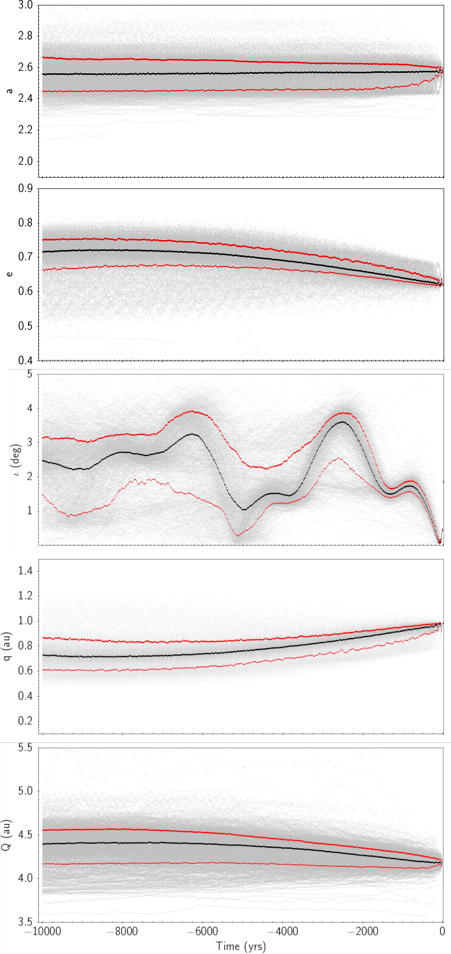
Figure 10: Orbital elements for the Winchcombe meteoroid over the previous ten thousand years, from the integration of 1000 particles using the IAS15 integrator (Rein & Spiegel, 2015). The black line is indicative of the median value, meanwhile, the red lines show the 1-sigma variation.

5 Strewn field

5.1 Atmospheric model

The atmospheric conditions and winds for the dark flight were modelled numerically using the Weather Research and Forecasting (WRF) model version 4.0 with dynamic solver ARW (Advanced Research WRF) (Skamarock et al., 2019). The weather models include wind speed, wind direction, pressure, temperature, and relative humidity at heights ranging up to 30 km. Three runs were processed, starting the weather simulation at different times before the meteorite fall, on 2021-02-28 at 6:00, 12:00, and 18:00 UTC. The 12:00 UTC profile is shown in Figure 11. Fortuitously, the atmospheric conditions were stable and all three times gave relatively similar profiles, which is not always the case for other falls (e.g. Devillepoix et al., 2018). The atmospheric models are available in Supplementary Materials.

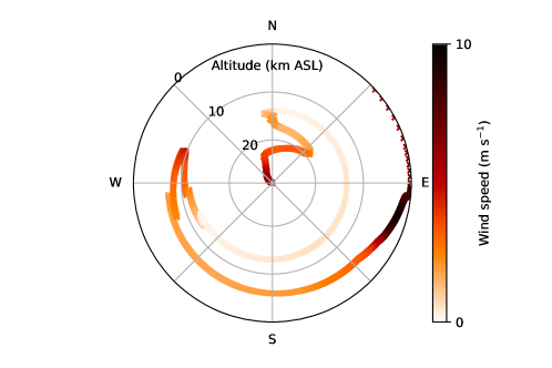
Figure 11: Wind model (speed and direction for a given altitude), extracted as a vertical profile at the location and time of the lowest visible bright flight measurement. Model integration started at 2021-02-12T12:00. The winds affecting this fall were very low, as the maximum wind encountered by the meteoroid during the dark flight was $\sim$10 m s^-1 coming from the East, at around 0.4 km altitude.

5.2 Dark flight

The 12:00 UTC wind model was used to predict where meteorites would land, based on the last observed bright flight state vector (Sec. 3), using the method of Towner et al. (2022) . We create Monte Carlo clones by varying the final observed state vector within uncertainty (Sec. 3), as well as meteorite physical parameters such as mass, shape and density (fixed at 2090 kg m^-3 based on recovered meteorite properties King et al. (2022)). The azimuth and altitude used for dark flight followed the original straight-line trajectory, prior to the deviation observed at 35 km, as the absolute amount and direction of the deviation could not be determined from single-station observations. The masses are randomly sampled logarithmically from $\sim$5 g to $\sim$0.8 kg, and shape coefficients drawn from a normal distribution that covers predominantly spherical and cylindrical shapes: $A=\mathcal{N}(\mu=1.4,\,\sigma^{2}=0.33)$ (Zhdan et al., 2007; Sansom et al., 2017). The drag is calculated dynamically as a function of the atmosphere and flight conditions via the Reynolds number (see Towner et al. (2022)). For this case, a model was also run for extreme non-aerodynamic shapes (A=2.7; tile-like Zhdan et al. (2007)) to extend the fall line to all recovered fragment locations (see discussion in section 5.2.1).

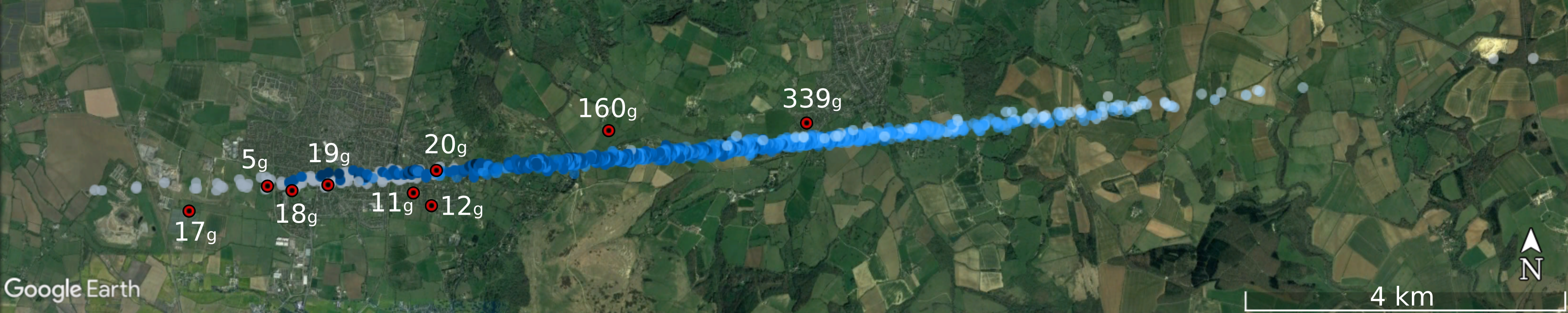
Figure 12: Fall line for the Winchcombe meteorite fall. Red points correspond to the location of the meteorites found with their estimated masses (Russell et al., 2022). Monte Carlo points from the darkflight simulation are blue shaded based on the assumed shape. In this case, the shape is the dominant parameter shifting the points along the fall line: dark blue are more brick-like and less aerodynamic in shape, while light blue is more sphere-like and aerodynamic shapes. Grey points to the west are from a custom model using an extreme, tile-like shape for reference.

The predicted strewn field is in reasonable agreement with the positions of the recovered meteorites (Fig. 12). Nonetheless, our modelling is unable to predict the lateral extent of the fall area. Below, we treat along and across the fall line shifts separately.

5.2.1 Along the fall line

The position of masses along the fall line is primarily controlled by the shape and the mass of the fragments (East-West direction in Fig. 12). When performing Monte Carlo dark flight simulations, these parameters are assumed a priori in order to predict where certain masses would fall (points in Fig. 12). Knowing the location and masses of recovered fragments with respect to these simulated stones can inform us of the approximate shape, impact speed, and flight time for each sample.

Cross-matching samples with simulations, the main mass found (Site 1 in Russell et al. (2022)) would have had a moderate shape coefficient of 1.4 to 1.5 (similar drag profile to a cylinder) and hit the ground at 46 to 49 m s^-1 after a dark flight free fall time of $\sim$4.5 minutes. The other large mass (160 g at site 5) likely had a shape coefficient of 1.5 to 1.7 and hit the ground at 35 to 40 m s^-1 after a flight time of $\sim$6 minutes. Smaller fragments would require extreme shapes to match the fall line (grey points in Fig. 12). In particular, the 16.5 g mass at Site 6 requires a shape coefficient of $\sim 2.7$ (as found by Čapek et al., 2021) and would have impacted at 17 to 19 m s^-1, after a $\sim$16 minute flight. An alternative explanation is that this fragment entered the dark flight phase at a higher altitude (consistent with 2-3 km before the end), as was in fact observed in the Hullavington video. The lateral deviation of this fragment from the line also supports a longer dark flight phase (see also section 5.2.2). The spread of recovered meteorites along the modelled fall line is consistent with differences in their physical characteristics, as well as the late fragmentation of the smaller stones.

5.2.2 Across the fall line

The position of masses across the fall line is primarily controlled by the state vector at the end of the bright flight (North-South direction in Fig. 12). The lateral spread of the Monte Carlo simulations due to uncertainties in this final state vector is $\sim$200 m (90 m s^-1). Some of the Winchcombe fragments were recovered outside of this area by up to $\sim$300 m on either side. This creates a $\sim$600 m corridor formed by the found masses. It should be noted that our $\sim$200 m wide predicted fall line is in the middle of this $\sim$600 m corridor. To account for the fragments lying outside the lateral spread of the Monte Carlo simulations, the various meteoritic fragments must have had differences in their final bright flight velocity vector that model uncertainties alone cannot account for. Strong evidence of this direction change process is evident in Fig. 3, in which the Hullavington viewpoint displays a projected deviation of $\sim$200 m. With a single viewpoint on the end of the bright flight trajectory, it is difficult to estimate the true spread of the fragments in 3D space. Nonetheless, an observed 200 m projected deviation could well explain a 500 m cross-line positional difference between different fragments if their flight was completely tracked to the ground.

Passey & Melosh (1980) have also proposed significant lateral velocities in fragments just after a breakup from studying strewn fields on Earth. These could be due to lift effects, bow shock interactions, centripetal separation of a rotating meteoroid, or transverse separation from reaching meteoroid crushing strengths (Passey & Melosh, 1980). These authors propose a spreading velocity proportional to the velocity at breakup such that $V_{spreading}=V_{breakup}\times\sqrt{C\times\rho_{a}/\rho_{m}}$, where here the atmospheric density and meteoroid density refer to those at breakup altitude, and $C$ is an empirical constant that ranges from 0.02 to 1.5 (based on strewn field analyses on Earth, Venus, and Mars; Passey & Melosh, 1980; Herrick & Phillips, 1994; Popova et al., 2007; Collins et al., 2022). For the final fragmentation of the Winchcombe meteoroid at 34.9 km, this relation predicts spreading velocities in the range of 2.5 - 22.5 m/s. This would account for a maximum deviation over the final 2.01 s of $\sim$45 m. The observed 200 m deviation and a minimum lateral velocity of 90 m/s would require $C$ values of over 30. Such high lateral spreading velocities are not however unreasonable. Both Boroviĉka & Kalenda (2003) for the Morávka fireball, and Docobo & Ceplecha (1999) for another fragmenting event, show spreading velocities of up to 300 m/s for observed fragments. These significantly higher values than represented in strewn field data show the energetic nature of the fragmentation processes that simple models of mere atmospheric loading cannot account for. The addition of any volatile materials in a carbonaceous-type meteoroid would be expected to exaggerate these effects. We note that the deviation occurred during a fragmentation event which released 28% of the remaining mass ($\sim 150$ g) into dust. We postulate that a preferential direction for the dust release might also explain the gain in transverse momentum.

A common assumption for fall area estimation is that the more precise the overall bright flight trajectory is, the smaller the search area will be. Although this is likely true, there is a catch: the individual fragments must be well observed from multiple sites at the end of the bright flight. Therefore, unless multi-station viewpoints are available at high-resolution (arc minute) and high sensitivity (down to magnitude 0^M), it is not possible to predict the width of meteorite fall line within less than a couple of hundreds of meters, no matter how precisely the upper trajectory is determined.

6 Discussion

The limited number of carbonaceous chondrites with known pre-atmospheric orbits is largely due to their poor survivability (Ceplecha & McCrosky, 1976). Carbonaceous chondrites are weak, so they fragment and ablate quickly in the Earth’s atmosphere (Ceplecha et al., 1998). To survive as a meteorite, their atmospheric trajectories require one or more specific properties: low entry speeds (approach from the antapex, i.e. opposite to the direction of Earth’s motion around the Sun), shallow entry angles, and large initial masses.

The first instrumentally observed carbonaceous chondrite meteorite fall, Tagish Lake, fell on 18 January 2000 at 16:43 UTC in a remote region of northern British Columbia, Canada (Brown et al., 2000). The meteorite was categorised as a C2-ungrouped carbonaceous chondrite with an initial mass of up to 200,000 kg. There were over 70 eyewitness reports, with 24 photographs and five videos of the dust cloud taken by observers within 1-2 mins after the event. It was also detected by infrared and optical sensors aboard US Department of Defense Satellites and the corresponding shock wave was detected by local seismic and infrasound stations (Brown et al., 2002). More than 500 meteorites were recovered, with the largest fragment 2.3 kg, and a total mass of 16.3 kg (Popova et al., 2011). The lack of direct ground-based optical recordings and reliance on classified satellite data mean that the orbit might contain systematic uncertainties that are not well understood (Devillepoix et al., 2019).

The Maribo meteorite fell on 17 January 2009, at 18:08:28 UTC in Denmark (Haack et al., 2012), and was identified as a CM2 meteorite with a calculated initial meteoroid mass of 2000$\pm$1000 kg (Borovička et al., 2019). There were 550 eyewitness reports and it was captured by a surveillance camera in southern Sweden, a photo from an all-sky fireball camera in the Netherlands, and by three all-sky meteor radars in Germany. The sonic boom was recorded by 11 seismometers and an infrasound station. Seven radiometers in the Czech Republic were able to measure the radiometric light curve, allowing for the first detailed ablation and fragmentation modelling of a carbonaceous meteorite fall.

The Sutter’s Mill meteorite fell on 22 April 2012, at 14:51:12 UTC in California and was identified as a CM2 carbonaceous chondrite with a calculated initial meteoroid mass of 20,000–80,000 kg (Jenniskens et al., 2012). It was observed by 3 Doppler weather radars, 2 infrasound stations, and 8 seismic stations, along with a set of three photographs from Nevada, and a few videos.

The most recent recorded carbonaceous meteorite fall, Flensburg, occurred on 12 September 2019, 12:50 UTC over northern Germany. It was identified as a C1-ungrouped carbonaceous chondrite with a calculated initial meteoroid mass of 10,000–20,000 kg (Borovička et al., 2021). There were 584 eyewitness reports and it was recorded by one AllSky6 camera and three dash cameras. A single meteorite of 24.5 g was recovered, and there was insufficient data to estimate the total mass or number of fragments.

Each of the four previous carbonaceous falls had high entry velocities ($>15$ km s^-1) and consequently experienced high dynamic pressures ($>1$ MPa) which caused mechanical disintegration of the weak bodies. The reason why any meteorites survived at all is that their pre-atmospheric masses were large ($>$1 t) and they had shallow entry angles ($<30^{\circ}$) (Table 6), allowing few meteorites to survive by chance while $>>99$% of the initial mass was destroyed. In contrast, Winchcombe experienced the most favourable entry conditions possible which enabled a significant amount of material from the smallest ever observed carbonaceous meteoroid to survive to the ground.

Name	Classification	Max	Initial Mass	Initial	Entry	Semi-major	$T_{J}$	Ref.
		Pressure	Range	Velocity	Angle	Axis
		(MPa)	(kg)	(km s-1)	(∘)	(AU)
Tagish Lake	C2(ungrouped)	2.2	50,000–200,000	15.8	16.5	$2.1\pm 0.2$	3.66	1
Maribo	CM2	5	1,000–3,000	28.3$\pm$0.3	31	$2.43\pm 0.12$	$2.95\pm 0.11$	2, 3
Sutter’s Mill	CM2	$>1$	20,000–80,000	28.6$\pm$0.6	26.3$\pm$0.5	$2.59\pm 0.35$	$2.81\pm 0.32$	4
Flensburg	C1(ungrouped)	2	10,000–20,000	19.43$\pm$0.05	24.4	$2.82\pm 0.03$	$2.89\pm 0.02$	5
Winchcombe	CM2	0.6	9–15	13.547$\pm$0.008	41.92$\pm$0.03	$2.586\pm 0.008$	$3.121\pm 0.006$	6, 7

Table 6: Physical and orbital properties of previous carbonaceous chondrite falls, in comparison to Winchcombe. The entry angle is reference to the horizontal. See references for details on falls and their orbits: (1) Brown et al. (2000), (2) Haack et al. (2012), (3) Borovička et al. (2019), (4) Jenniskens et al. (2012), (5) Borovička et al. (2021), (6) King et al. (2022), (7) this work.

7 Conclusions

Winchcombe is the first meteorite recovered in the UK in 30 years, the first carbonaceous chondrite recovered in the UK, and the first instrumentally observed meteorite fall in the UK.

The main scientific takeaways of this work are:

• The Winchcombe meteoroid entered with favourable entry parameters (low velocity and entry angle) to avoid $>$1 MPa dynamic pressures; an uncommon range of conditions that were necessary for the survival of weak carbonaceous material. So far, amongst meteorites with measured orbits, only multi-ton objects have been proven to drop carbonaceous chondrites. In the more traditional meteorite dropping size (decimetre), a strong velocity bias exists against the survival of carbonaceous material. Winchcombe is the first evidence that survival of smaller cabronaceous bodies is possible, but only for objects approaching from the antapex which by rule have the slowest entry velocities.

• The surviving fragments experienced a significant flight vector change before entering dark flight, obtaining a velocity kick perpendicular to a straight-line trajectory of at least 90 m s^-1. The physical phenomenon that caused this could not be definitely determined, but we investigate several possibilities that require further study. The deviation resulted in fragments being scattered beyond the nominal error boundaries of the fall area. Without detailed observations at both high-resolution and high sensitivity of the very end of the bright flight, it may not be possible to predict meteorite fall positions to better than a few hundred metres.

• The recent ejection of Winchcombe from a parent asteroid as measured by the cosmic-ray exposure ages ($\sim 0.3$ Myr) is longer or contemporary with the time spent as a Near-Earth Object inferred from its orbit (0.035—0.24 Myr, 0.08 Myr nominal). This indicates a minimal time delay between ejection from its parent body and the insertion into near-Earth space.

• The analysis of the Winchcombe fireball involved five independent optical observation networks. This validates the need for standard data exchange procedures, as proposed by Rowe et al. (2020), in order to enable a quick turnaround time from the time the fireball happens to when a fall area is calculated.

8 Supplementary materials

Supplementary materials have been uploaded as a Zenodo record at http://doi.org/10.5281/zenodo.6685719. It contains fireball images (including calibration data), astrometry tables in Global Fireball Exchange standard, the trajectory report file, and the wind profiles.

References

- Alexander et al. (2012) Alexander, C. O., Bowden, R., Fogel, M., et al. 2012, Science, 337, 721
- Astropy Collaboration et al. (2013) Astropy Collaboration, Robitaille, T. P., Tollerud, E. J., et al. 2013, A&A, 558, A33, doi: 10.1051/0004-6361/201322068
- Bischoff (1998) Bischoff, A. 1998, Meteoritics & Planetary Science, 33, 1113
- Borovička (2014) Borovička, J. 2014, in Proceedings of the International Meteor Conference, Poznan, Poland, 22-25 August 2013, 101–105
- Boroviĉka & Kalenda (2003) Boroviĉka, J., & Kalenda, P. 2003, Meteoritics & Planetary Science, 38, 1023
- Borovička et al. (2019) Borovička, J., Popova, O., & Spurnỳ, P. 2019, Meteoritics & Planetary Science, 54, 1024
- Borovička et al. (2020) Borovička, J., Spurnỳ, P., & Shrbenỳ, L. 2020, The Astronomical Journal, 160, 42
- Borovička et al. (2013) Borovička, J., Tóth, J., Igaz, A., et al. 2013, Meteoritics & Planetary Science, 48, 1757
- Borovička et al. (2015) Borovička, J., Spurnỳ, P., Šegon, D., et al. 2015, Meteoritics & Planetary Science, 50, 1244
- Borovička et al. (2015) Borovička, J., Spurný, P., & Brown, P. 2015, Small Near-Earth Asteroids as a Source of Meteorites, ed. P. Michel, F. E. DeMeo, & W. F. Bottke (University of Arizona Press), 257–280, doi: 10.2458/azu_uapress_9780816532131-ch014
- Borovička et al. (2011) Borovička, J., Abe, S., Shrbenỳ, L., Spurnỳ, P., & Bland, P. A. 2011, Publications of the Astronomical Society of Japan, 63, 1003
- Borovička et al. (2021) Borovička, J., Bettonvil, F., Baumgarten, G., et al. 2021, \maps, 56, 425, doi: 10.1111/maps.13628
- Borovička et al. (2021) Borovička, J., Bettonvil, F., Baumgarten, G., et al. 2021, Meteoritics & Planetary Science, 56, 425
- Borovička et al. (2019) Borovička, J., Popova, O., & Spurný, P. 2019, Meteoritics and Planetary Science, 54, 1024, doi: 10.1111/maps.13259
- Bronshten (1983) Bronshten, V. A. 1983, Physics of Meteoric Phenomena, Geophysics and Astrophysics Monographs (Dordrecht, Netherlands: Reidel)
- Brown et al. (2002) Brown, P. G., Revelle, D. O., Tagliaferri, E., & Hildebrand, A. R. 2002, \maps, 37, 661, doi: 10.1111/j.1945-5100.2002.tb00846.x
- Brown et al. (2000) Brown, P. G., Hildebrand, A. R., Zolensky, M. E., et al. 2000, Science, 290, 320, doi: 10.1126/science.290.5490.320
- Campbell-Burns & Kacerek (2014) Campbell-Burns, P., & Kacerek, R. 2014, WGN, Journal of the International Meteor Organization, 42, 139
- Ceplecha (1961) Ceplecha, Z. 1961, Bulletin of the Astronomical Institutes of Czechoslovakia, 12, 21
- Ceplecha et al. (1998) Ceplecha, Z., Borovička, J., Elford, W. G., et al. 1998, Space Science Reviews, 84, 327
- Ceplecha & McCrosky (1976) Ceplecha, Z., & McCrosky, R. 1976, Journal of Geophysical Research, 81, 6257
- Ceplecha & Revelle (2005) Ceplecha, Z., & Revelle, D. O. 2005, Meteoritics & Planetary Science, 40, 35, doi: 10.1111/j.1945-5100.2005.tb00363.x
- Colas et al. (2015) Colas, F., Zanda, B., Bouley, S., et al. 2015, in European Planetary Science Congress, EPSC2015–800
- Colas et al. (2020) Colas, F., Zanda, B., Bouley, S., et al. 2020, A&A, 644, A53, doi: 10.1051/0004-6361/202038649
- Collins et al. (2022) Collins, G. S., Newland, E. L., Schwarz, D., et al. 2022, JGR-Planets, accepted, doi: https://doi.org/10.1002/essoar.10509245.1
- Daly et al. (2020) Daly, L., McMullan, S., Rowe, J., et al. 2020, in European Planetary Science Congress, EPSC2020–705, doi: 10.5194/epsc2020-705
- Devillepoix et al. (2019) Devillepoix, H. A., Bland, P. A., Sansom, E. K., et al. 2019, Monthly Notices of the Royal Astronomical Society, 483, 5166
- Devillepoix et al. (2018) Devillepoix, H. A. R., Sansom, E. K., Bland, P. A., et al. 2018, \maps, 53, 2212, doi: 10.1111/maps.13142
- Devillepoix et al. (2019) Devillepoix, H. A. R., Bland, P. A., Sansom, E. K., et al. 2019, MNRAS, 483, 5166, doi: 10.1093/mnras/sty3442
- Devillepoix et al. (2020) Devillepoix, H. A. R., Cupák, M., Bland, P. A., et al. 2020, Planet. Space Sci., 191, 105036, doi: 10.1016/j.pss.2020.105036
- Docobo & Ceplecha (1999) Docobo, J. A., & Ceplecha, Z. 1999, A&AS, 138, 1, doi: 10.1051/aas:1999263
- Gattacceca et al. (2022) Gattacceca, J., McCubbin, F. M., Grossman, J., et al. 2022, Meteoritics & Planetary Science, 57, 2102
- Granvik & Brown (2018) Granvik, M., & Brown, P. 2018, Icarus, 311, 271
- Gritsevich et al. (2014) Gritsevich, M., Lyytinen, E., Moilanen, J., et al. 2014, in Proceedings of the International Meteor Conference, Giron, France, 18–21
- Haack et al. (2012) Haack, H., Grau, T., Bischoff, A., et al. 2012, Meteoritics & Planetary Science, 47, 30
- Herrick & Phillips (1994) Herrick, R. R., & Phillips, R. J. 1994, Icarus, 112, 253, doi: 10.1006/icar.1994.1180
- Howie et al. (2017a) Howie, R. M., Paxman, J., Bland, P. A., et al. 2017a, Experimental Astronomy, 43, 237, doi: 10.1007/s10686-017-9532-7
- Howie et al. (2017b) —. 2017b, \maps, 52, 1669, doi: 10.1111/maps.12878
- Jenniskens et al. (2012) Jenniskens, P., Fries, M. D., Yin, Q.-Z., et al. 2012, Science, 338, 1583, doi: 10.1126/science.1227163
- Johnston et al. (2018) Johnston, C. O., Stern, E. C., & Wheeler, L. F. 2018, Icarus, 309, 25
- King et al. (2022) King, A. J., Daly, L., Rowe, J., et al. 2022, Science Advances, 8, eabq3925
- Krot et al. (2015) Krot, A., Nagashima, K., Alexander, C., et al. 2015, Asteroids IV, 635
- Krot et al. (2014) Krot, A. N., Keil, K., Scott, E. R. D., Goodrich, C. A., & Weisberg, M. K. 2014, in Meteorites and Cosmochemical Processes, ed. A. M. Davis, Vol. 1 (Elsevier), 1–63
- Marchi et al. (2009) Marchi, S., Delbo’, M., Morbidelli, A., Paolicchi, P., & Lazzarin, M. 2009, MNRAS, 400, 147, doi: 10.1111/j.1365-2966.2009.15459.x
- Marty (2012) Marty, B. 2012, Earth and Planetary Science Letters, 313, 56
- Matlovič et al. (2022) Matlovič, P., Pisarčíková, A., Tóth, J., et al. 2022, Monthly Notices of the Royal Astronomical Society, 513, 3982
- McCrosky et al. (1971) McCrosky, R. E., Posen, A., Schwartz, G., & Shao, C.-Y. 1971, Journal of Geophysical Research, 76, 4090
- Meech & Raymond (2020) Meech, K., & Raymond, S. N. 2020, in Planetary Astrobiology, ed. V. S. Meadows, G. N. Arney, B. E. Schmidt, & D. J. Des Marais (University of Arizona Press), 325, doi: 10.2458/azu_uapress_9780816540068
- Passey & Melosh (1980) Passey, Q. R., & Melosh, H. J. 1980, Icarus, 42, 211, doi: 10.1016/0019-1035(80)90072-X
- Picone et al. (2002) Picone, J., Hedin, A., Drob, D. P., & Aikin, A. 2002, Journal of Geophysical Research: Space Physics, 107, SIA
- Pizzarello et al. (2006) Pizzarello, S., Cooper, G., & Flynn, G. 2006, Meteorites and the early solar system II, 1, 625
- Popova et al. (2011) Popova, O., Borovička, J., Hartmann, W. K., et al. 2011, Meteoritics and Planetary Science, 46, 1525, doi: 10.1111/j.1945-5100.2011.01247.x
- Popova et al. (2007) Popova, O., Hartmann, W. K., Nemtchinov, I. V., Richardson, D. C., & Berman, D. C. 2007, Icarus, 190, 50, doi: 10.1016/j.icarus.2007.02.022
- Rein & Spiegel (2015) Rein, H., & Spiegel, D. S. 2015, MNRAS, 446, 1424, doi: 10.1093/mnras/stu2164
- Rowe et al. (2020) Rowe, J., Daly, L., McMullan, S., et al. 2020, in European Planetary Science Congress, EPSC2020–856
- Russell et al. (2022) Russell, S., King, A., Daly, L., & others. 2022, \maps, this issue
- Sansom et al. (2017) Sansom, E. K., Rutten, M. G., & Bland, P. A. 2017, AJ, 153, 87, doi: 10.3847/1538-3881/153/2/87
- Scott & Krot (2014) Scott, E., & Krot, A. 2014, Meteorites and cosmochemical processes, 1, 65
- Shober et al. (2021) Shober, P. M., Sansom, E. K., Bland, P. A., et al. 2021, The Planetary Science Journal, 2, 98
- Shober et al. (2021) Shober, P. M., Sansom, E. K., Bland, P. A., et al. 2021, \psj, 2, 98, doi: 10.3847/PSJ/abde4b
- Skamarock et al. (2019) Skamarock, W. C., Klemp, J. B., Dudhia, J., et al. 2019, A description of the advanced research WRF version 4, Tech. rep., NCAR Technical Note NCAR/TN-556+STR, doi: 10.5065/1dfh-6p97
- Spurnỳ et al. (2020) Spurnỳ, P., Borovička, J., & Shrbenỳ, L. 2020, Meteoritics & Planetary Science, 55, 376
- Stewart et al. (2013) Stewart, W., Pratt, A. R., & Entwisle, L. 2013, WGN, Journal of the International Meteor Organization, 41, 84
- Suttle et al. (2021) Suttle, M., King, A., Schofield, P., Bates, H., & Russell, S. 2021, Geochimica et Cosmochimica Acta, 299, 219
- Toliou et al. (2021) Toliou, A., Granvik, M., & Tsirvoulis, G. 2021, MNRAS, doi: 10.1093/mnras/stab1934
- Towner et al. (2022) Towner, M. C., Jansen-Sturgeon, T., Cupak, M., et al. 2022, \psj, 3, 44, doi: 10.3847/PSJ/ac3df5
- Trigo-Rodríguez et al. (2019) Trigo-Rodríguez, J. M., Rimola, A., Tanbakouei, S., Soto, V. C., & Lee, M. 2019, Space Science Reviews, 215, 1
- Čapek et al. (2021) Čapek, D., Kohout, T., Pachman, J., Macke, R., & Koten, P. 2021, in European Planetary Science Congress, EPSC2021–306, doi: 10.5194/epsc2021-306
- Vida et al. (2021a) Vida, D., Brown, P. G., Campbell-Brown, M., et al. 2021a, Icarus, 354, 114097
- Vida et al. (2020) Vida, D., Gural, P. S., Brown, P. G., Campbell-Brown, M., & Wiegert, P. 2020, Monthly Notices of the Royal Astronomical Society, 491, 2688
- Vida et al. (2018) Vida, D., Mazur, M., Šegon, D., et al. 2018, WGN, Journal of the International Meteor Organization, 46, 71
- Vida et al. (2016) Vida, D., Zubović, D., Šegon, D., Gural, P., & Cupec, R. 2016, Proceedings of the IMC2016, Egmond, The Netherlands
- Vida et al. (2021b) Vida, D., Šegon, D., Gural, P. S., et al. 2021b, Monthly Notices of the Royal Astronomical Society, 506, 5046
- Vida et al. (2022) Vida, D., Brown, P. G., Devillepoix, H. A., et al. 2022, Nature Astronomy, 1
- Wheeler et al. (2017) Wheeler, L. F., Register, P. J., & Mathias, D. L. 2017, Icarus, 295, 149
- Zhdan et al. (2007) Zhdan, I., Stulov, V., Stulov, P., & Turchak, L. 2007, Solar System Research, 41, 505