Symmetry-resolved entanglement in fermionic systems with dissipation

Abstract

We investigate symmetry-resolved entanglement in out-of-equilibrium fermionic systems subject to gain and loss dissipation, which preserves the block-diagonal structure of the reduced density matrix. We derive a hydrodynamic description of the dynamics of several entanglement-related quantities, such as the symmetry-resolved von Neumann entropy and the charge-imbalance-resolved fermionic negativity. We show that all these quantities admit a hydrodynamic description in terms of entangled quasiparticles. While the entropy is dominated by dissipative processes, the resolved negativity is sensitive to the presence of entangled quasiparticles, and it shows the typical “rise and fall” dynamics. Our results hold in the weak-dissipative hydrodynamic limit of large intervals, long times and weak dissipation rates.

¹ Walter Burke Institute for Theoretical Physics, Caltech, Pasadena, CA 91125, USA
² Department of Physics and IQIM, Caltech, Pasadena, CA 91125, USA
³ SISSA and INFN Sezione di Trieste, via Bonomea 265, 34136 Trieste, Italy
⁴ International Centre for Theoretical Physics (ICTP), Strada Costiera 11, 34151 Trieste, Italy
⁵ Dipartimento di Fisica dell’Università di Pisa and INFN, Sezione di Pisa, I-56127 Pisa, Italy

1 Introduction

The study of entanglement dynamics is of fundamental importance to understand the process of thermalisation or the lack thereof in out-of-equilibrium quantum many-body systems [1, 2, 3, 4, 5]. In one-dimensional integrable systems the entanglement dynamics after a quantum quench is amenable of a hydrodynamic description within the framework of the famous quasiparticle picture [6, 7, 8, 9, 11, 12, 10]. Specifically, the entanglement dynamics is determined by the ballistic propagation of entangled pairs of quasiparticles. Importantly, recent progress with cold-atom and trapped-ion systems allows us to experimentally measure entanglement-related quantities [13, 14, 15, 16] and their dynamics.

The starting point for all entanglement-related quantities is the reduced density matrix $\rho_{A}$ of a subsystem $A$. For example, the entanglement Rényi entropies are defined as

$$S_{n}=\frac{1}{1-n}\log(\mathrm{Tr}\rho^{n}_{A}).$$ (1)

The limit $n\to 1$ gives the von Neumann entropy as

$$S_{1}=-\mathrm{Tr}\rho_{A}\log\rho_{A}.$$ (2)

The Rényi entropies and the von Neumann entropy are proper entanglement measures for bipartite pure states only. If the system is in a bipartite mixed state, neither the von Neumann entropy nor the mutual information are bona fide entanglement measures. In these situations, for fermionic systems, one can use the logarithmic negativity or the fermionic logarithmic negativity (see section 4 for precise definitions).

Recently, there has been growing interest in the interplay between symmetries and entanglement. Specifically, if the system possesses a global symmetry, for instance, particle number conservation, the reduced density matrix exhibits a block structure, each block corresponding to a different symmetry sector [17, 18, 19]. The question how the different symmetry sectors contribute to the entanglement entropies attracted a lot of attention, also experimentally [14, 22, 21, 20]. On the theoretical side, several works focused on the symmetry-resolved entropies, especially in field theory [18, 19, 23, 24, 25, 26, 27, 28, 29, 30, 31, 32, 33, 34, 35, 36, 38, 39, 40, 41, 42, 43, 44, 45, 37] and spin chains both at equilibrium [46, 47, 55, 56, 53, 49, 50, 51, 52, 48, 54, 57, 59, 60, 61, 62, 63, 65, 64, 66, 58], as well as in out-of-equilibrium situations [68, 69, 70, 72, 71, 73, 74, 75]. The charge-imbalance-resolved negativity has been investigated at equilibrium [76, 77, 78], and also its out-of-equilibrium dynamics was addressed [79, 80, 81]. Remarkably, the resolved negativity can be accessed experimentally [20, 21].

Still, most of the effort so far focussed on closed quantum many-body systems. Since in generic systems the interaction with an environment is unavoidable, it is crucial to understand the behaviour of entanglement and symmetry-resolved entanglement in out-of-equilibrium open quantum many-body systems. This is in general a challenging task, and results are available only in few situations, for instance, within the simplified framework of the Lindblad master equations [82]. For quadratic Lindblad master equations, i.e., for free-fermion and free-boson models with linear Lindblad operators, the out-of-equilibrium dynamics of the Rényi entropies, and of the mutual information can be understood within the quasiparticle picture [83, 84, 85]. This result holds in the weak-dissipative hydrodynamic limit of long times and large subsystems, and weak dissipation. Moreover, some results are available for the fermionic logarithmic negativity as well. For instance, the dynamics of the negativity in free-fermion systems subject to gain and loss dissipation was investigated in Ref. [86]. Interestingly, due to the mixedness of the global state, the negativity is not related to the Rényi mutual information, in contrast with the unitary case [87]. The dynamics of both the von Neumann entropy and the negativity in the presence of localised losses has been studied recently [88, 89]. Relatedly, it has been shown that in free-fermion models in contact with localised thermal baths, which are treated within the Lindblad formalism, the mutual information exhibits a logarithmic scaling [90]. Finally, symmetry-resolved entanglement in open quantum many-body systems has received comparatively little attention, although some numerical and perturbative results are available [21].

Here we build a quasiparticle picture for several symmetry-resolved entanglement measures in free fermions subject to gain and loss dissipation. Such dissipation shall violate the particle number conservation, i.e. the $U(1)$ symmetry. However, as we will discuss below, the local Lindblad jump operators, which define the dissipative mechanism, preserve the block-diagonal structure of the reduced density matrix. We can refer to this scenario as a weak $U(1)$ symmetry [93, 91, 21, 94, 95, 92]. Specifically, we provide analytic results for both the symmetry-resolved von Neumann entropy, and the charge-imbalance-resolved fermionic negativity. Similar to the non-resolved von Neumann entropy, the symmetry-resolved one is dominated by volume-law terms, which originate from dissipation. These are accompanied by terms that retain information about entangled quasiparticles. Precisely, these terms have the same structure as in the non-dissipative case. However, the entanglement content of the correlated quasiparticles is renormalised by the dissipative processes, and it vanishes exponentially at long times, reflecting how dissipation destroys genuine quantum correlation. While the entropies are dominated by dissipative contributions, we show that the fermionic symmetry-resolved negativity is determined by the entangled quasiparticles. Indeed, the resolved negativity exhibits the typical “rise and fall” dynamics, i.e., it grows at short times $t\lesssim 1/\gamma^{\pm}$, with $\gamma^{\pm}$ the dissipation rates, and it vanishes at long times. Interestingly, for generic gain/loss processes the symmetry-resolved entropies do not exhibit a time delay, meaning that they are different from zero for any $t>0$, as already numerically observed in [21]. This reflects that different charge sectors are immediately “populated” due to the presence of the dissipation. This represents a crucial difference with respect to the case without dissipation [69].

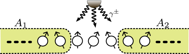
Figure 1: Schematic view of our setup. A fermionic chain is subject to gain and loss dissipation: Fermions are added or removed incoherently at rates $\gamma^{\pm}$. The incoherent processes act on each site of the chain independently. The chain is initially prepared in a low-entangled state $|\Psi_{0}\rangle$. Here we choose as initial states the fermionic Néel state $|\mathrm{N}\rangle$ and the Majumdar-Ghosh state $|\mathrm{D}\rangle$. The chain evolves under the action of the tight-binding fermionic Hamiltonian and the Lindblad operators. We are interested in the symmetry-resolved entanglement entropy of a subregion $A$ with the rest. We also consider the charge-imbalance-resolved negativity between two equal intervals $A_{1}$ and $A_{2}$ of length $\ell$ and placed at distance $d$.

The manuscript is organised as follows. We start in section 2 reviewing quantum quenches in free-fermion models without dissipation. In section 3 we introduce the dissipation and its treatment within the framework of the Lindblad master equation. In section 4 we introduce the symmetry-resolved von Neumann entropy and the resolved negativity, discussing also their calculation in free-fermion models. Section 5 is devoted to the presentation of our main results. Specifically, in section 5.1 we discuss the charged moments of the reduced density matrix, which are essential ingredients to compute the symmetry-resolved entropy. In section 5.2 we discuss how to obtain the symmetry-resolved entropy and several useful approximations. In section 6 we present our results for the charge-imbalance-resolved negativity. In particular, we discuss the charged moments of the partial time-reversed reduced density matrix, and the resolved negativity. In section 7 we provide numerical benchmarks. Specifically, in section 7.1 and section 7.2 we discuss the charged moments and the symmetry-resolved entropies, respectively. In section 7.3 we address the validity of the quadratic approximation for the charged moments. Finally, in section 7.4 we discuss the scaling in the weak-dissipative hydrodynamic limit. In particular, we highlight the presence of logarithmic corrections, which arise from the charge fluctuations between the subsystem and the rest. These are revealed in the scaling of the number entropy. In section 7.5 we benchmark our results for the resolved negativity. We present our conclusions in section 8.

2 Quantum quenches in free-fermion models

We consider the fermionic chain defined by the Hamiltonian

$$H=\frac{1}{2}\sum_{j=1}^{L}(c^{\dagger}_{j}c_{j+1}+c^{\dagger}_{j+1}c_{j}).$$ (3)

Here $L$ is the chain size, $c_{j}^{\dagger}$ and $c_{j}$ are canonical fermionic creation and annihilation operators with anticommutation relations $\{c^{\dagger}_{j},c_{l}\}=\delta_{jl}$ and $\{c_{j},c_{l}\}=0$. The Hamiltonian (3) is diagonalised by going to Fourier space defining the fermionic operators $b_{k}:=\frac{1}{\sqrt{L}}\sum_{j}e^{ikj}c_{j}$, with the quasimomentum $k=2\pi p/L$ and $p=0,1,\dots,L-1$. The Hamiltonian (3) becomes diagonal as

$$H=\sum_{k}\varepsilon(k)b_{k}^{\dagger}b_{k},\quad\mathrm{with}\,\,\varepsilon(k):=\cos(k).$$ (4)

Here we defined the single-particle energy levels $\varepsilon(k)$. In the following we are considering the thermodynamic limit $L\to\infty$. For later convenience we define the group velocity of the fermionic excitations $v(k)$ as

$$v(k):=\varepsilon^{\prime}(k)=d\varepsilon(k)/dk.$$ (5)

We focus on the nonequilibrium dynamics after the quench from the fermionic Néel state $|\mathrm{N}\rangle$ and Majumdar-Ghosh (dimer) state $|\mathrm{D}\rangle$, defined as

$$|\mathrm{N}\rangle:=\prod_{j=1}^{L/2}c^{\dagger}_{2j}|0\rangle$$ (6)

$$|\mathrm{D}\rangle:=\prod_{j=1}^{{L/2}}\frac{c^{\dagger}_{2j}-c^{\dagger}_{2j-1}}{\sqrt{2}}|0\rangle,$$ (7)

with $|0\rangle$ the fermionic vacuum state.

Let us now discuss the quench protocol. At time $t=0$ we prepare the system in $|\mathrm{N}\rangle$ or $|\mathrm{D}\rangle$. At $t>0$ the chain undergoes unitary dynamics under the Hamiltonian (3). The fermionic correlation function $\widetilde{C}_{jl}$ is the central object to address entanglement related quantities in free-fermion systems [96]. The matrix $\widetilde{C}_{jl}$ is defined as

$$\widetilde{C}_{jl}:=\langle c^{\dagger}_{j}c_{l}\rangle.$$ (8)

Here $\langle\cdot\rangle$ denotes the expectation value calculated with the time-dependent wavefunction. The dynamics of the correlation function $\widetilde{C}_{jl}(t)$ (cf. (8)) after the quench from both the Néel state and the Majumdar-Ghosh state can be derived analytically (see for instance, Ref. [80]). For the Néel state it is straightforward to obtain

$$\widetilde{C}_{jl}=\frac{1}{2}\delta_{jl}+\frac{1}{2}(-1)^{l}\int_{-\pi}^{\pi}\frac{dk}{2\pi}e^{ik(j-l)+2it\varepsilon(k)}=\frac{1}{2}\delta_{jl}+\frac{1}{2}(-1)^{l}J_{j-l}(2t),$$ (9)

where $J_{x}(t)$ is the Bessel function of the first kind. In (9) is to stress that the dynamics is unitary.

It is useful to exploit the invariance of the Néel state and the Majumdar-Ghosh state under translation by two sites. Thus, we rewrite (8) as

$$\left(\begin{array}[]{cc}\widetilde{C}_{2j,2l}&\widetilde{C}_{2j,2l-1}\\ \widetilde{C}_{2j-1,2l}&\widetilde{C}_{2j-1,2l-1}\end{array}\right):=\left\langle\left(\begin{array}[]{c}c_{2j}^{\dagger}\\ c_{2j-1}^{\dagger}\end{array}\right)\left(\begin{array}[]{cc}c_{2l}&c_{2l-1}\end{array}\right)\right\rangle=\int_{-\pi}^{\pi}\frac{dk}{2\pi}e^{2ik(j-l)}\hat{t}(k),$$ (10)

where now $j,l$ label the position of a two-site unit cell and $\hat{t}(k)$ is a two-by-two matrix. The factor $2$ in the exponent in the integral in (10) reflects translation invariance by two sites. From (9), one obtains the matrix $\hat{t}(k)$ for the Néel state as

$$\hat{t}_{\mathrm{N}}(k)=\frac{1}{2}\left(\begin{array}[]{cc}1+e^{2it\varepsilon(k)}&e^{2it\varepsilon(k)+ik}\\ -e^{2it\varepsilon(k)-ik}&1-e^{2it\varepsilon(k)}\end{array}\right).$$ (11)

For the Majumdar-Ghosh state we use $\hat{t}_{\mathrm{D}}(k)$ given by [97, 69]

$$\hat{t}_{\mathrm{D}}(k)=\frac{1}{2}\begin{pmatrix}&f_{+}(k,t)&-g^{*}(k,t)\\ &-g(k,t)&f_{-}(k,t)\end{pmatrix}$$ (12)

with

$$f_{\pm}(k,t)=1\pm\sin(k)\sin(2\varepsilon(k)t)$$ (13)

$$g(k,t)=e^{-ik}(\cos(k)+i\sin(k)\cos(2\varepsilon(k)t)),$$ (14)

where $\varepsilon(k)$ is given in (4).

3 Lindblad evolution in the presence of gain and loss dissipation

Let us now discuss the out-of-equilibrium dynamics in the tight-binding chain (cf. (3)) with fermionic gain and loss processes. To describe these dissipative processes, we employ the formalism of quantum master equations [82]. Precisely, the Lindblad equation describes the time-dependent density matrix $\rho_{t}$ of the full system as

$$\frac{d\rho_{t}}{dt}=\mathcal{L}(\rho_{t}):=-i[H,\rho_{t}]+\sum_{j=1}^{L}\sum_{\alpha=\pm}\left(L_{j,\alpha}\rho_{t}L_{j,\alpha}^{\dagger}-\frac{1}{2}\left\{L_{j,\alpha}^{\dagger}L_{j,\alpha},\rho_{t}\right\}\right)\,.$$ (15)

Here, $\{x,y\}$ is the anticommutator. The dissipation is modelled by $L_{j,\alpha}$, which are known as Lindblad jump operators. For gain and loss processes they are defined as $L_{j,-}:=\sqrt{\gamma^{-}}c_{j}$ and $L_{j,+}:=\sqrt{\gamma^{+}}c_{j}^{\dagger}$, with $\gamma^{\pm}$ the gain and loss rates. As it is clear from Eq. (15), incoherent absorption and emission of fermions happen independently at each site of the chain. This choice of the jump operators, $L_{j,\pm}$, falls into the category of weak symmetries, i.e. the generator of the master equation as a whole commutes with the symmetry operation, while each of the jump operator does not commute individually with the symmetry [91]. Their main feature is that they preserve the block-diagonal form of the reduced density matrix. Indeed, if the system is prepared in an initial symmetric state (like $\ket{N}$ or $\ket{D}$), the system state remains supported in the same symmetric eigenspace (with a given charge) when no jumps take place. On the other hand, when the first jump $L_{j_{1},\pm}$ occurs at time $t_{1}$, the system is transformed to another eigenspace with different charge. If we interpret Eq. (15) as a set of quantum trajectories, each one corresponding to the solution of a stochastic Schrödinger equation, the quantum trajectories are symmetric at all times: a single quantum jump only changes the number of particles by an integer number, but the total number of particles is conserved along each trajectory [94].

For quadratic fermionic Hamiltonians, it is straightforward to obtain from (15) the dynamics of the fermionic two-point function $C_{jl}=\langle c^{\dagger}_{j}c_{l}\rangle=\mathrm{Tr}(\rho_{t}c^{\dagger}_{j}c_{l})$. Indeed, $C(t)$ is given by [84]

$$C(t)=e^{t\Lambda}C(0)e^{t\Lambda^{\dagger}}+\int_{0}^{t}dz\,e^{(t-z)\,\Lambda}\Gamma^{+}e^{(t-z)\,\Lambda^{\dagger}}\,.$$ (16)

Here $\Lambda=ih-1/2(\Gamma^{+}+\Gamma^{-})$, where for the tight-binding chain we have $h_{jl}=1/2(\delta_{j+1,l}+\delta_{j,l+1})$. In (16), $\Gamma^{\pm}$ are $L\times L$ matrices defined as $\Gamma^{\pm}_{jl}=\gamma^{\pm}\delta_{jl}$. Since $\Gamma_{jl}^{\pm}$ are diagonal, $C_{jl}$ can be rewritten in terms of the correlation matrix $\widetilde{C}_{jl}(t)$ describing the dynamics in the absence of dissipation, i.e., with $\gamma^{\pm}=0$ (cf. (8)). Precisely, one has

$$C_{jl}=n_{\infty}(1-b)\mathds{1}_{jl}+b\widetilde{C}_{jl},\quad b:=e^{-(\gamma^{+}+\gamma^{-})t},\,n_{\infty}:=\frac{\gamma^{+}}{\gamma^{+}+\gamma^{-}},$$ (17)

where $\mathds{1}_{jl}$ is the identity matrix element. Moreover, Eq. (17) suggests that it is convenient to modify the matrix $\hat{t}(k)$ (cf. (10)) defining $\hat{t}^{\prime}(k)$ as

$$\hat{t}^{\prime}(k)=n_{\infty}(1-b)\mathds{1}_{2}+b\hat{t}(k),$$ (18)

where $\mathds{1}_{2}$ is the $2\times 2$ identity matrix, and $\hat{t}(k)$ is the original matrix defined in (10). The correlator $C_{jl}$ is then obtained as

$$C_{jl}=\int_{-\pi}^{\pi}\frac{dk}{2\pi}e^{2ik(j-l)}\hat{t}^{\prime}(k).$$ (19)

Here $\hat{t}^{\prime}(k)$ is given in (18), with $\hat{t}(k)$ defined in (11) and (12).

4 Symmetry-resolved entanglement

In this section we overview the definitions of our quantities of interest, namely the symmetry-resolved entanglement entropies and the charge-imbalance-resolved negativity. We focus on quantum systems with an internal $U(1)$ symmetry generated by a local operator $Q$. For the tight-binding chain in (3) this corresponds to the conservation of the number of fermions. The $U(1)$ symmetry implies that $[\rho,Q]=0$. If the system is bipartite in two complementary subsystems $A$ and $B$, since the operator $Q$ is sum of local terms, $Q$ is decomposed as the sum of operators acting separately on the degrees of freedom of $A$ and $B$, i. e., $Q=Q_{A}+Q_{B}$. By taking the trace over $B$ in $[\rho,Q]=0$ we obtain that $[\rho_{A},Q_{A}]=0$, implying that the reduced density matrix $\rho_{A}$ is block diagonal. The different blocks correspond to a different charge sector with eigenvalue $q$ of $Q_{A}$. We have

$$\rho_{A}=\oplus_{q}\Pi_{q}\rho_{A}=\oplus_{q}[p(q)\rho_{A}(q)],$$ (20)

where $\Pi_{q}$ projects over the eigenspace with eigenvalue $q$ and we defined $p(q)=\mathrm{Tr}\left(\Pi_{q}\rho_{A}\right)$ as the probability that $Q_{A}$ has value $q$. Here we normalise $\rho_{A}(q)$ such that $\mathrm{Tr}{\rho_{A}}(q)=1$. In the following section we introduce several entanglement-related quantities that can be defined from $\rho_{A}(q)$. This allows to understand how the different charge sectors of the reduced density matrix contribute to the entanglement. We stress again that this block-diagonal structure of $\rho_{A}$ is preserved by the dissipative evolution in Eq. (15) within our choice of $L_{j,\pm}$ [91, 93, 21].

4.1 Symmetry-resolved entropies

Let us introduce the symmetry-resolved Rényi and von Neumann entropy. The latter is the entropy calculated from the different charge sectors of the reduced density matrix as

$$S_{1}(q):=-\mathrm{Tr}[\rho_{A}(q)\log(\rho_{A}(q))],$$ (21)

where, again, $\rho_{A}(q)$ is the normalised block of $\rho_{A}$ corresponding to the charge $q$. To proceed, we plug Eq. (20) into the definition of the von Neumann entropy, to obtain the decomposition as

$$S_{1}=\sum_{q}p(q)S_{1}(q)-\sum_{q}p(q)\log(p(q)):=S^{(c)}+S^{(\mathrm{num})},$$ (22)

where $p(q)$ is the probability of measuring charge $q$ in the subsystem. The first term in (22) quantifies the average of the von Neumann entropy of each charge sector, and it is called configurational entropy[14, 48, 50]. On the other hand, $S^{(\mathrm{num})}$ measures the charge fluctuations between subsystem $A$ and its complement, and it is called number entropy [14, 59, 60, 62, 61, 63].

Notice that from $\rho_{A}(q)$ one can define the symmetry-resolved Rényi entropies [46] as

$$S_{n}(q):=\frac{1}{1-n}\log\mathrm{Tr}[\rho^{n}_{A}(q)].$$ (23)

Here, however, we only consider the von Neumann entropy.

We now discuss how to compute the symmetry-resolved entropy. In general, its computation, for instance in a field-theory setup, requires the spectrum of the symmetry-resolved reduced density matrix. This is challenging to extract because the projector $\Pi_{q}$ is a nonlocal operator. Here we follow a different strategy, which was put forward in Ref. [18, 19], and which we now outline. The central objects of this approach are the charged moments, $Z_{r}(\alpha)$. They are defined as

$$Z_{r}(\alpha)=\mathrm{Tr}[\rho_{A}^{r}e^{i\alpha Q_{A}}].$$ (24)

By performing the Fourier transform of the charged moments, we get the moments of the reduced density matrix in a given charge sector, i.e.,

$$\mathcal{Z}_{r}(q):=\mathrm{Tr}(\Pi_{q}\rho^{r})=\int_{-\pi}^{\pi}\frac{d\alpha}{2\pi}e^{-iq\alpha}Z_{r}(\alpha),\quad p(q)=\mathcal{Z}_{1}(q),$$ (25)

where $\Pi_{q}$, again, is the projector, which selects the block of the reduced density matrix that corresponds to value of the charge $q$. The symmetry-resolved Rényi entropies $S_{r}(q)$ with Rényi index $r$ are defined as

$$S_{r}(q)=\frac{1}{1-r}\log\left(\frac{\mathcal{Z}_{r}(q)}{\mathcal{Z}_{1}^{r}(q)}\right),\quad S_{1}(q)=\lim_{r\to 1}S_{r}(q),$$ (26)

where the symmetry-resolved von Neumann entropy $S_{1}$ is obtained as usual by taking the limit $r\to 1$ of $S_{r}$. Finally, for the free-fermion Hamiltonian (3) one can write the charged moments in terms of the two-point fermionic correlation function as [18]

$$\log(Z_{r}(\alpha))=\mathrm{Tr}\log[C_{A}^{r}e^{i\alpha}+(1-C_{A})^{r}],$$ (27)

where $C_{A}$ (cf. Eq. (8)) is the fermionic correlation matrix restricted to part $A$ of the chain.

4.2 Charge-imbalance-resolved fermionic negativity

Let us now consider the logarithmic negativity. We start by reviewing the definition of the partial transpose and its relation to the time-reversal transformation. Let us consider a density matrix $\rho_{A}$ in which $A$ is further partitioned as $A=A_{1}\cup A_{2}$ (see Fig. 1), where $A_{1}$ ($A_{2}$) is an interval of length $\ell_{1}$ ($\ell_{2}$). We can write

$$\rho_{A}=\sum_{ijkl}\braket{e^{1}_{i},e^{2}_{j}}{\rho_{A}}{e^{1}_{k},e^{2}_{l}}\ket{e_{i}^{1},e_{j}^{2}}\bra{e^{1}_{k},e^{2}_{l}},$$ (28)

where $\ket{e_{j}^{1}}$ and $\ket{e_{k}^{2}}$ are orthonormal bases for the Hilbert spaces of $A_{1}$ and $A_{2}$, respectively. The partial transpose $\rho^{T_{1}}_{A}$ of $\rho_{A}$ with respect to $A_{1}$ is defined as

$$(\ket{e_{i}^{1},e_{j}^{2}}\bra{e^{1}_{k},e^{2}_{l}})^{T_{1}}:=\ket{e_{k}^{1},e_{j}^{2}}\bra{e^{1}_{i},e^{2}_{l}}.$$ (29)

The negativity is written in terms of the negative eigenvalues of $\rho_{A}^{T_{1}}$, and it is essentially the trace norm of $\rho_{A}^{T_{1}}$. In terms of its eigenvalues $\lambda_{i}$, the trace norm of $\rho_{A}^{T_{1}}$ can be rewritten as

$$\mathrm{Tr}|\rho_{A}^{T_{1}}|=\sum_{i}|\lambda_{i}|=\sum_{\lambda_{i}>0}|\lambda_{i}|+\sum_{\lambda_{i}<0}|\lambda_{i}|=1+2\sum_{\lambda_{i}<0}|\lambda_{i}|,$$ (30)

where in the last equality we used the normalisation $\sum_{i}\lambda_{i}=1$. Moreover, in the absence of negative eigenvalues, $\mathrm{Tr}|\rho_{A}^{T_{1}}|=1$ and the negativity vanishes. For a bosonic system, it is known [98] that the partial transpose is equivalent to the time-reversal partial transpose. This allows one to calculate the negativity in terms of the covariance matrix in bosonic systems, such as the harmonic chain [99].

For fermionic systems, the standard negativity is not easily computed in terms of the two-point correlation function, because the partial transpose is not a Gaussian operator [100, 101]. On the other hand, the fermionic negativity [102], which is defined from the time-reversed partial transpose, can be computed. To introduce the fermionic time-reversed partial transpose it is convenient to introduce Majorana fermion operators $w_{j}$ as

$$w_{2j-1}=c_{j}+c^{\dagger}_{j},\quad w_{2j}=i(c_{j}-c^{\dagger}_{j}),$$ (31)

with $c_{j}$ the original fermions. The density matrix in the Majorana representation takes the form

$$\rho_{A}=\sum_{\begin{subarray}{c}\kappa,\tau\\ |\kappa|+|\tau|=\mathrm{even}\end{subarray}}M_{\kappa,\tau}w_{m_{1}}^{\kappa_{m_{1}}}\dots w_{2m_{\ell_{1}}}^{\kappa_{2m_{\ell_{1}}}}w_{m^{\prime}_{1}}^{\tau_{m^{\prime}_{1}}}\dots w_{2m^{\prime}_{\ell_{2}}}^{\tau_{2m^{\prime}_{\ell_{2}}}}.$$ (32)

Here, $w^{0}_{x}=\mathds{1}$, $w^{1}_{x}=w_{x}$, $\kappa_{i},\tau_{j}\in\{0,1\}$, and $\kappa$ ($\tau$) is a $2m_{\ell_{1}}$-component vector ($2m^{\prime}_{\ell_{2}}$) with entries $0,1$ and with norm $|\kappa|=\sum_{j}\kappa_{j}$ ($|\tau|=\sum_{j}\tau_{j}$). The constraint on the parity of $|\kappa|+|\tau|$ is due to the fact that we require the density matrix to commute with the total fermion-number parity operator. In (32) $M_{\kappa,\tau}$ are complex numbers. Using Eq. (32), the partial time-reversed (TR) transpose $\rho^{R_{1}}_{A}$ with respect to the subsystem $A_{1}$ is defined by

$$\rho_{A}^{R_{1}}=\sum_{\begin{subarray}{c}\kappa,\tau\\ |\kappa|+|\tau|=\mathrm{even}\end{subarray}}i^{|\kappa|}M_{\kappa,\tau}w_{m_{1}}^{\kappa_{m_{1}}}\dots w_{2m_{\ell_{1}}}^{\kappa_{2m_{\ell_{1}}}}w_{m^{\prime}_{1}}^{\tau_{m^{\prime}_{1}}}\dots w_{2m^{\prime}_{\ell_{2}}}^{\tau_{2m^{\prime}_{\ell_{2}}}}.$$ (33)

The matrix $\rho_{A}^{R_{1}}$ is not necessarily Hermitian, and may have complex eigenvalues, although $\mathrm{Tr}\rho_{A}^{R_{1}}=1$. Still the eigenvalues of the operator $[\rho_{A}^{R_{1}}(\rho_{A}^{R_{1}})^{\dagger}]$ are all real. Following Refs. [102, 103, 104] we define the fermionic negativity as

$${\cal E}:=\log\mathrm{Tr}\sqrt{\rho_{A}^{R_{1}}(\rho_{A}^{R_{1}})^{\dagger}}.$$ (34)

One can also define the (fermionic) Rényi logarithmic negativities ${\cal E}_{r}=\log(R_{r})$ with $R_{r}$ given as

$$R_{r}=\begin{cases}\mathrm{Tr}(\rho_{A}^{R_{1}}(\rho_{A}^{R_{1}})^{\dagger}\dots\rho_{A}^{R_{1}}(\rho_{A}^{R_{1}})^{\dagger}),&\quad r\quad\mathrm{even},\\ \mathrm{Tr}(\rho_{A}^{R_{1}}(\rho_{A}^{R_{1}})^{\dagger}\dots\rho_{A}^{R_{1}}),&\quad r\quad\mathrm{odd}.\end{cases}$$ (35)

The negativity can be obtained as $\displaystyle\mathcal{E}=\lim_{r_{e}\to 1}\log(R_{r_{e}})$, where $r_{e}$ denotes an even integer [102].

We can adapt the approach discussed in section 4.1 to the computation of the charged moments of the time-reversed (TR) partial transpose obtaining

$$N_{r}(\alpha)=\begin{cases}\mathrm{Tr}(\rho_{A}^{R_{1}}(\rho_{A}^{R_{1}})^{\dagger}\dots\rho_{A}^{R_{1}}(\rho_{A}^{R_{1}})^{\dagger}e^{i{Q}_{A}\alpha}),&\quad r\quad\mathrm{even},\\ \mathrm{Tr}(\rho_{A}^{R_{1}}(\rho_{A}^{R_{1}})^{\dagger}\dots\rho_{A}^{R_{1}}e^{i{Q}_{A}\alpha}),&\quad r\quad\mathrm{odd}.\end{cases}$$ (36)

A Fourier transform allows us to derive the moments of the TR partial transpose ${\mathcal{Z}}_{R_{1},r}$ as

$$\mathcal{Z}_{R_{1},r}(q)=\displaystyle\int_{-\pi}^{\pi}\frac{d\alpha}{2\pi}e^{-i\alpha q}N_{r}(\alpha),\quad p(q)=\displaystyle\int_{-\pi}^{\pi}\frac{d\alpha}{2\pi}e^{-i\alpha q}N_{1}(\alpha),$$ (37)

from which we define the ratios $R_{r}(q)$ and the charge-imbalance-resolved negativity ${\mathcal{E}}(q)$ as

$$R_{r}(q)=\frac{\mathcal{Z}_{R_{1},r}(q)}{p^{r}(q)},\qquad\mathcal{E}(q)=\lim_{r_{e}\to 1}\log\left(\frac{{\mathcal{Z}}_{R_{1},r_{e}}(q)}{p^{r_{e}}(q)}\right).$$ (38)

Let us stress that the replica limit for $R_{r_{e}}(q)$ requires an analytic continuation $r_{e}\to 1$ from the even sequences $R_{r_{e}}$, whereas in the denominator we can set $r\to 1$.

Let us now discuss how to compute the charged moments $N_{r}(\alpha)$ in free-fermion systems. The covariance matrix $\Gamma$ is the central object to compute the charged moments and the symmetry-resolved negativity. $\Gamma$ is defined as

$$\Gamma_{jl}=\mathds{1}-2C_{jl},\quad j,l\in A,$$ (39)

where $\mathds{1}$ is the identity matrix restricted to subsystem $A=A_{1}\cup A_{2}$, and $C_{jl}$ is the fermionic correlation matrix (17). If the subsystem $A$ is made of two intervals as $A=A_{1}\cup A_{2}$ (see Fig. 1), we can decompose $\Gamma$ as

$$\Gamma=\begin{pmatrix}\Gamma_{11}&\Gamma_{12}\\ \Gamma_{21}&\Gamma_{22}\end{pmatrix},$$ (40)

where $\Gamma_{11}$ and $\Gamma_{22}$ are the reduced covariance matrices of the two subsystems $A_{1}$ and $A_{2}$, respectively, while $\Gamma_{12}$ and $\Gamma_{21}^{\dagger}$ contain the cross correlations between them. By simple Gaussian states manipulations, the covariance matrices $\Gamma_{\pm}$ associated with $\rho^{R_{1}}_{A}$ and $(\rho^{R_{1}}_{A})^{\dagger}$ (cf. (33) for their definitions) are obtained as

$$\Gamma_{\pm}=\begin{pmatrix}-\Gamma_{11}&\pm i\Gamma_{12}\\ \pm i\Gamma_{21}&\Gamma_{22}\end{pmatrix}.$$ (41)

Here we are interested in $N_{r}(\alpha)$ defined as

$$N_{r}(\alpha)=\mathrm{Tr}[(\rho_{A}^{R_{1}}(\rho_{A}^{R_{1}})^{\dagger})^{r/2}e^{iQ_{A}\alpha}],$$ (42)

where $r$ is an even integer. We also consider $N_{1}(\alpha)$ defined as

$$N_{1}(\alpha)=\mathrm{Tr}[\rho_{A}^{R_{1}}e^{iQ_{A}\alpha}].$$ (43)

To proceed we need the covariance matrix $\Gamma_{\mathrm{x}}$ associated with the normalised composite density operator $\rho_{\mathrm{x}}=\rho_{A}^{R_{1}}(\rho_{A}^{R_{1}})^{\dagger}/Z_{\mathrm{x}}$. This is given as [80]

$$\Gamma_{\mathrm{x}}=(\mathds{1}+\Gamma_{+}\Gamma_{-})^{-1}(\Gamma_{+}+\Gamma_{-}),$$ (44)

where the normalisation factor is $Z_{\mathrm{x}}=\mathrm{Tr}(\Gamma_{\mathrm{x}})=\mathrm{Tr}(\rho_{A}^{2})$.

To proceed, let us define the charged Rényi negativities ${\cal E}_{r}(\alpha)$ (for even $r$) as

$${\cal E}_{r}(\alpha):=\log(N_{r}(\alpha))=-2i\alpha\ell+\mathrm{Tr}\log\left[\left(\frac{\mathds{1}-\Gamma_{\mathrm{x}}}{2}\right)^{r/2}+e^{i\alpha}\left(\frac{\mathds{1}+\Gamma_{\mathrm{x}}}{2}\right)^{r/2}\right]\\ +\frac{r}{2}\mathrm{Tr}\log\left[C_{A}^{2}+(\mathds{1}-C_{A})^{2}\right],$$ (45)

where $N_{r}(\alpha)$ are defined in (42) and we have set $\ell_{1}=\ell_{2}=\ell$. Here $C_{A}$ is the restricted fermionic correlation matrix, i.e., $C_{jl}$ with $j,l\in A$. Now, Eq. (45) can be rewritten as

$${\cal E}_{r}(\alpha)=-2i\alpha\ell+\sum_{j=1}^{2\ell}\log\left[\left(\frac{1-\nu_{j}^{\mathrm{x}}}{2}\right)^{r/2}+e^{i\alpha}\left(\frac{1+\nu_{j}^{\mathrm{x}}}{2}\right)^{r/2}\right]\\ +\frac{r}{2}\sum_{j=1}^{2\ell}\log\left[\zeta_{j}^{2}+(1-\zeta_{j})^{2}\right],$$ (46)

where $\nu_{j}^{\mathrm{x}}$ are eigenvalues of the matrices $\Gamma_{\mathrm{x}}$ (44), and $\zeta_{j}$ are the eigenvalues of the fermion correlation matrix $C_{A}$ introduced in the section 2. The charged negativity ${\cal E}(\alpha)$ is defined as

$${\cal E}(\alpha):=\lim_{r\to 1}{\cal E}_{r}(\alpha),\quad\mathrm{with}\,\,r\,\,\mathrm{even}.$$ (47)

Finally, let us observe that $N_{1}(\alpha)$ is written in terms of the eigenvalues $\nu^{+}_{j}$ of $\Gamma_{+}$ (41)

$$\log(N_{1}(\alpha))=-2i\alpha\ell+\sum_{j=1}^{2\ell}\log\left[\left(\frac{1-\nu^{+}_{j}}{2}\right)+e^{i\alpha}\left(\frac{1+\nu^{+}_{j}}{2}\right)\right].$$ (48)

The strategy to compute the charge-imbalance-resolved negativity is to perform the Fourier transform of the quasiparticle prediction for $\log(N_{r}(\alpha))$ and $\log(N_{1}(\alpha))$.

5 Quasiparticle picture for symmetry-resolved entropies

In this section we derive the quasiparticle picture for the symmetry-resolved entropies. In section 5.1 we focus on the charged moments of the reduced density matrix, whereas in section 5.2 we present our results for the symmetry-resolved von Neumann entropy. In section 5.2 we also discuss some useful approximations that are needed to derive analytically the behaviour of the resolved entropies.

5.1 Charged moments of the reduced density matrix

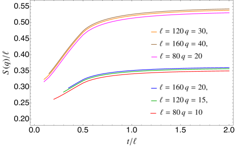
Figure 2: Effect of gain and loss dissipation in the symmetry-resolved von Neumann entropy $S(q)$. We show results for the quench from the Néel state in the tight-binding chain. We plot the density of entropy $S(q)/\ell$ versus rescaled time $t/\ell$ for different charge sectors $q$. Here we fix $q/\ell=1/8$ and $q/\ell=1/4$. To ensure the weak-dissipative hydrodynamic limit the dissipation rates $\gamma^{\pm}$ are fixed as $\gamma^{-}=1/\ell$, $\gamma^{+}=5/(100\ell)$.

Here we discuss the quasiparticle picture for the charged moments (27) for the quench from the Néel state (6) and dimer state (7). We consider the weakly dissipative hydrodynamic limit, which corresponds to $\ell,t\to\infty$, $\gamma^{\pm}\to 0$, at fixed and arbitrary $t/\ell$ and $\gamma^{\pm}\ell$, with $\ell$ the length of the subsystem $A$.

Since we are interested in the dynamics of Gaussian states, the system is fully characterised at any time after the quench by its two-point correlation functions. In the absence of pairing terms like $c^{\dagger}c^{\dagger}$ or $cc$ in the Hamiltonian at time $t=0$, the relevant covariance matrix is $C_{jl}$ (cf. (17)). Again, the correlation matrix in the presence of gain/loss dissipation is simply related to the dynamical correlation function $\widetilde{C}_{jl}$ (cf. (10)) for the quench without dissipation. To determine the quasiparticle picture for the charged moments, it is convenient to employ the representation of the fermionic correlator in (19) and (10) (11). To proceed, we formally expand (27) as

$$\log(Z_{r}(\alpha))=\sum_{j=0}^{\infty}c_{j}\mathrm{Tr}\,C_{A}^{j},$$ (49)

where $C_{A}$ is $C_{jl}$ (cf. (17)) with $j,l\in A$, and the coefficients $c_{j}$ are the coefficients of the Taylor expansion of $\log[x^{r}e^{i\alpha}+(1-x)^{r}]$ around $x=0$.

By following the same steps of Ref. [86], we can find the quasiparticle picture for the charged moments. Specifically, we first consider the expansion (49). Thus, the problem is reduced to that of determining the hydrodynamic behaviour of $\mathrm{Tr}\,C_{A}^{j}$ for arbitrary $j$. This last step can be performed by using the multidimensional version of the stationary phase approximation [105]. By closely following the same steps as in [86], we obtain for both the quench from the Néel state and the dimer state that

$$\log(Z_{r}(\alpha))=\ell\int\frac{dk}{2\pi}\left[\mathrm{max}(1-2|v(k)|t/\ell,0)h^{\mathrm{mix}}_{r}(\alpha,k)+\mathrm{min}(2|v(k)|t/\ell,1)h^{\mathrm{q}}_{r}(\alpha,k)\right],$$ (50)

where $v(k)=\sin(k)$, i.e., the same group velocity of the fermions in the non-dissipative case. In (50) we introduced the two contributions $h_{r}^{\mathrm{mix}}(\alpha,k)$ and $h_{r}^{\mathrm{q}}(\alpha,k)$ defined as

$$h_{r}^{\mathrm{mix}}=\mathrm{Tr}\,h_{r}(\alpha,\hat{t}^{\prime}(k)),$$ (51)

$$h_{r}^{\mathrm{q}}=h_{r}(\alpha,\rho_{t}(k)).$$ (52)

Here the function $h_{r}(\alpha,x)$ is defined as

$$h_{r}(\alpha,x)=\log(e^{i\alpha}x^{r}+(1-x)^{r}).$$ (53)

The term (51) is of purely dissipative origin and it vanishes in the limit $\gamma^{\pm}\to 0$. Precisely, $h^{\mathrm{mix}}_{r}(\alpha,k)$ corresponds to the charged moments obtained from (27) by replacing $C_{A}$ with the full-system correlator. Notice that in (51) the trace is over the two-by-two matrix $\hat{t}^{\prime}(k)$ (cf. (18)). The term $h_{r}^{\mathrm{q}}$ in (50) is a “quantum” one, meaning that it is determined by both the dissipative and the unitary part of the evolution (15). In the limit $\gamma^{\pm}\to 0$ this term gives the result of the quasiparticle picture in the non dissipative case. Importantly, $h^{\mathrm{q}}_{r}(\alpha,k)$ depends only on the fermion density $\rho_{t}(k)$. In the absence of dissipation $\rho_{t}(k)$ does not depend on time, which is not the case at nonzero $\gamma^{\pm}$. For quenches in the tight-binding chain in the presence of gain/loss dissipation the time-evolved density $\rho_{t}(k)$ is obtained as [84]

$$\rho_{t}(k)=e^{-\gamma(k)t}\rho_{0}(k)+\frac{\alpha(k)}{\gamma(k)}(1-e^{-\gamma(k)t}).$$ (54)

Here we have

$$\gamma(k)=\gamma^{+}+\gamma^{-},\quad\alpha(k)=\gamma^{+}.$$ (55)

As it is clear from (55) for the quench from the Néel state and the dimer state $\gamma(k)$ and $\alpha(k)$ do not depend on the quasimomentum $k$. This simplification holds for the gain/loss dissipation but it is not expected for the generic linear dissipation [84, 85]. In (54) $\rho_{0}(k)$ is the density of fermionic quasiparticles that fully characterises the Generalised Gibbs Ensemble (GGE) in the absence of dissipation. Specifically, $\rho_{0}(k)$ is computed as $\rho_{0}(k)=\langle\psi_{0}|c^{\dagger}_{k}c_{k}|\psi_{0}\rangle$. For the quench from the Néel and the dimer state, a straightforward calculation gives the densities $\rho^{\mathrm{N}}_{0}(k)$ and $\rho^{\mathrm{D}}_{0}(k)$ as

$$\rho^{\mathrm{N}}_{0}(k)=\frac{1}{2},\quad\rho_{0}^{\mathrm{D}}(k)=|\cos(k)|.$$ (56)

Finally, by using the explicit form of $\hat{t}^{\prime}(k)$ (cf. (18)) for the Néel and the dimer quench, we obtain that $h^{\mathrm{mix}}_{r}$ is the same for both of them, and it reads as

$$h^{\mathrm{mix}}_{r}(\alpha,k)=\frac{h_{r}(\alpha,n_{0})+h_{r}(\alpha,n_{1})}{2}.$$ (57)

Here $n_{0}$ and $n_{1}$ are given as

$$n_{0}=\frac{\alpha(k)}{\gamma(k)}(1-e^{-\gamma(k)t}),\quad n_{1}=e^{-\gamma(k)t}+\frac{\alpha(k)}{\gamma(k)}(1-e^{-\gamma(k)t}),$$ (58)

where $\gamma(k)$ and $\alpha(k)$ are given in (55). Notice that $n_{0}$ is obtained from (54) by setting $\rho_{0}(k)=0$ and $n_{1}$ by fixing $\rho_{0}(k)=1$. This reflects that at $t=0$ for both the Néel state and the dimer state half of the eigenvalues of the correlation matrix $C_{jl}$ (cf. (8)) are zero and half are one. They do not depend on time in the absence of dissipation. For gain/loss dissipation, the eigenvalues evolve independently according to (54). It is also interesting to observe that we can rewrite (50) as

$$\log(Z_{r}(\alpha))=\int\frac{dk}{2\pi}\Big{\{}\ell h_{r}^{\mathrm{mix}}(\alpha,k)+\min(2|v(k)|t,\ell)\big{[}h_{r}^{\mathrm{q}}(\alpha,k)-h_{r}^{\mathrm{mix}}(\alpha,k)\big{]}\Big{\}}.$$ (59)

From (59) it is clear that $h_{r}^{\mathrm{mix}}$ plays a twofold role. Specifically, $h_{r}^{\mathrm{mix}}$ gives a volume-law contribution (first term in (59)) which does not contain information about the dynamics of the quasiparticles. On the other hand, $h_{r}^{\mathrm{mix}}$ also appears with a minus sign in the second term in (59), which is the “quantum” one because it is the only one surviving in the limit $\gamma^{\pm}\to 0$.

Let us now discuss some limits of $\log(Z_{r}(\alpha))$. First, at $t=0$ since $h_{r}(\alpha,0)=0$ and $h_{r}(\alpha,1)=i\alpha$, one has that $\log(Z_{r}(\alpha))=i\alpha\ell/2$. For $t\to\infty$, one has that $n_{0},n_{1}\to\alpha(k)/\gamma(k)=n_{\infty}$ (cf. (17)) and $\rho_{t}\to n_{\infty}$. This implies that the second term in (59) vanishes and finally one obtains $\log(Z_{r}(\alpha))\to\ell h_{r}^{\mathrm{mix}}(\alpha,n_{\infty})$.

5.2 Computing the symmetry-resolved entropies

To determine the quasiparticle picture for the symmetry-resolved entropies $S_{r}(q)$ (cf. (26)), one has to employ the quasiparticle picture for the charged moments $\log(Z_{r}(\alpha))$ in (25) and perform the Fourier transform. This is in general a challenging task, although closed-form expressions have been obtained in the nondissipative case [69]. Clearly, the Fourier transform in (25) can be performed numerically and we report the analytical predictions for the symmetry-resolved entropies in Fig. 2. However, this computation suffers from a numerical instability in solving the integral, and for this reason we omit the result for short time.

Another strategy is to use a saddle point approximation. Indeed, in (25) one has to assume $q\propto\ell$ in order to have non trivial results. We have

$${\mathcal{Z}}_{r}(q)=\int_{-\pi}^{\pi}\frac{d\alpha}{2\pi}e^{\ell h_{r}(\alpha)},$$ (60)

where we defined $h_{r}(\alpha)$ as

$$h_{r}(\alpha)=-i\frac{q}{\ell}\alpha+\int_{-\pi}^{\pi}\frac{dk}{2\pi}\Big{\{}h^{\mathrm{mix}}_{r}(\alpha,k)+\mathrm{min}(2|v|t/\ell,1)\big{[}h^{\mathrm{q}}_{r}(\alpha,k)-h^{\mathrm{mix}}(\alpha,k)\big{]}\Big{\}}.$$ (61)

The saddle point condition for $\alpha$ reads as

$$\partial_{\alpha}h_{r}(\alpha)\Big{|}_{\alpha=\alpha^{*}}=0.$$ (62)

Since the integration over $k$ in (61) can be performed analytically, the resulting saddle point condition for $\alpha^{*}$ can be effectively solved numerically. Moreover, analytic solutions of (61) are also possible, although the obtained expressions are cumbersome, and we do not report them. Instead, we now discuss some features of the solution $\alpha^{*}$.

In the absence of dissipation, $\alpha^{*}$ is a complex number and the presence of a nonzero real part leads to a delay in the evolution of the symmetry-resolved entropies, i.e., the entropies start to be nonzero for $t>t_{d}$, with $t_{d}$ the delay time [69]. Specifically, for each value of the charge $q$ we have that $\alpha^{*}$ in the non-dissipative situation is given as

$$\alpha^{*}=i\log\left(\frac{\mathcal{J}(t)-2\Delta q/\ell}{\mathcal{J}(t)+2\Delta q/\ell}\right),\quad\mathrm{with}\,\,\Delta q:=q-\frac{\ell}{2}.$$ (63)

Here we defined

$$\mathcal{J}(t):=\int_{-\pi}^{\pi}\frac{dk}{2\pi}\min(2|v(k)|t,\ell).$$ (64)

In the presence of gain and loss dissipation the delay effect is suppressed, as it was already shown in [21].

For simplicity, we focus on a quench from the Néel state $|\mathrm{N}\rangle$. First, the saddle point condition (62) has three solutions. By a standard saddle point analysis [105], we observe that the only physical solution describing the exact lattice computations are the ones with zero real part for any time $t$.

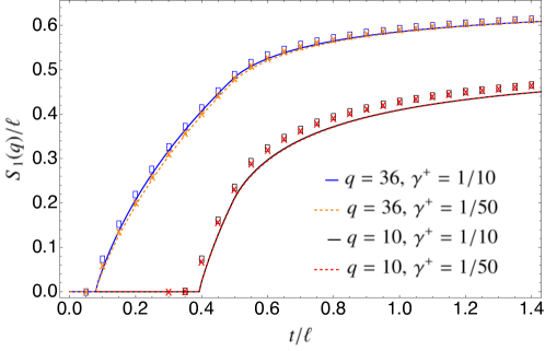
Figure 3: Time-delay in the dynamics of the symmetry-resolved von Neumann entropy with pure gain ($\gamma^{-}=0$). We plot $S_{1}(q)/\ell$ versus the rescaled time $t/\ell$, and fixed $\ell=80$, for the quench from the fermionic Néel state in the tight binding chain. The different lines are the results obtained from the quasiparticle picture for different values of the charge $q$ and dissipation $\gamma^{+}$, using the saddle point approximation. For some values of $t/\ell$ we report the numerical value of the symmetry-resolved entropy obtained through exact simulations of the dynamics (symbols). We clearly observe a delay time in agreement with Eq. (65), which does not depend on the dissipative term $\gamma^{+}$.

In the limit $\gamma^{+}\to 0$ ($\gamma^{-}\to 0$), i.e. pure loss or pure gain, we still find a delay time for $q>\ell/2$ ($q<\ell/2$). Indeed, in this case the saddle point condition has two solutions and, at short times $t\leq t_{d}$, the dominant solution of the saddle point condition gives a complex entropy which physically means that it averages to zero. As in the non-dissipative case, one finds that the delay time is obtained by solving the equation

$${\mathcal{J}}(t)-2\frac{|\Delta q|}{\ell}=0,\quad\Delta q=q-\frac{\ell}{2}.$$ (65)

In Fig. 3 we report the behaviour of the symmetry-resolved entropy using the saddle point approximation in the presence of pure gain and we show that, for $q<\ell/2$ it displays a delay, which is also confirmed by the exact lattice computations.

Having solved, for instance numerically, the saddle-point constraint (62), ${\mathcal{Z}}_{r}(q)$ for $t>t_{d}$ is given as

$${\mathcal{Z}}_{r}(q)=e^{\ell h_{r}(\alpha^{*})}\sqrt{\frac{1}{2\pi\ell|h_{r}^{\prime\prime}(\alpha^{*})|}},$$ (66)

where $\alpha^{*}$ is the solution of (62) with $\mathrm{Re}(\alpha^{*})=0$.

Another useful strategy to gain insights into the symmetry-resolved entropies is to use a quadratic approximation, by expanding the charged moments around $\alpha=0$. One obtains

$$\log(Z_{r}(\alpha))\simeq\log(Z_{r}(0))+i\alpha\mathcal{B}^{(1)}_{r}-\frac{\alpha^{2}}{2}\mathcal{B}^{(2)}_{r},$$ (67)

where

$$\mathcal{B}^{(1)}_{r}=\partial_{\alpha}\log(Z_{r}(\alpha))\Big{|}_{\alpha=0},\quad\mathcal{B}^{(2)}_{r}=\partial^{2}_{\alpha}\log(Z_{r}(\alpha))\Big{|}_{\alpha=0}.$$ (68)

With this quadratic expansion, we can perform the Fourier transform in (25). We obtain

$$\mathcal{Z}_{r}(q)=Z_{r}(0)e^{-\frac{(q-\mathcal{B}^{(1)}_{r})^{2}}{2\mathcal{B}^{(2)}_{r}}}\frac{1}{\sqrt{2\pi\mathcal{B}^{(2)}_{r}}}.$$ (69)

This approximation is valid only until $\Delta q=q-\mathcal{B}^{(1)}_{r}$ is ${\mathcal{O}}(\sqrt{\mathcal{B}^{(2)}_{r}})$, or, in other words, for small fluctuations $\Delta q$. Within this approximation, the corresponding symmetry-resolved entropies read

$$S_{r}(q)=S_{r}-\frac{1}{2}\log(2\pi)-\frac{1}{2(1-r)}\log\frac{\mathcal{B}^{(2)}_{r}}{(\mathcal{B}^{(2)}_{1})^{r}}-\frac{(q-\mathcal{B}^{(1)}_{r})^{2}}{2(1-r)}\left[\frac{1}{\mathcal{B}^{(2)}_{r}}-\frac{r}{\mathcal{B}^{(2)}_{1}}\right].$$ (70)

From Eq. (70), we can also predict the asymptotic value of the symmetry-resolved entropies for $t\to\infty$ at leading order in $\ell$. For a Néel state, we obtain

$$S_{1}(q)=-\ell n_{\infty}\log(n_{\infty})-\ell(1-n_{\infty})\log(1-n_{\infty})-1/2\log(2\pi\ell)-1/2\log((1-n_{\infty})n_{\infty})\\ +\frac{\tanh^{-1}(1-2n_{\infty})\left(-2\ell n_{\infty}^{2}q+\ell n_{\infty}(n_{\infty}(\ell+2n_{\infty}-3)+1)+(2n_{\infty}-1)q^{2}\right)}{\ell(n_{\infty}-1)n_{\infty}}\\ -\frac{(\ell n_{\infty}-q)^{2}}{2\ell n_{\infty}(1-n_{\infty})}.$$ (71)

Now, Eq. (71) predicts a volume-law scaling $\propto\ell$, and a subleading logarithmic one $\propto\log(\ell)$. Importantly, Eq. (71) relies on the validity of the quadratic approximation (70).

It is also interesting to derive the number entropy $S^{\mathrm{(\mathrm{num})}}$ (cf. (22)) within the quadratic approximation. It is obtained from $p(q)=\mathcal{Z}_{1}(q)$, and it is defined as

$$S^{(\mathrm{num})}=-\sum_{q}p(q)\log(p(q)).$$ (72)

By using the quadratic approximation for $\mathcal{Z}_{1}(q)$ (cf. (69)), we obtain that

$$p(q)=\frac{1}{\sqrt{\pi}}\frac{1}{\sqrt{2\ell\rho_{t}(1-\rho_{t})-2\mathcal{J}^{\prime}(t)(\rho_{t}-n_{0})^{2}}}\exp\left({-\frac{(q-\ell\rho_{t})^{2}}{2\ell\rho_{t}(1-\rho_{t})-2\mathcal{J}^{\prime}(t)(\rho_{t}-n_{0})^{2}}}\right),$$ (73)

where we defined $\mathcal{J}^{\prime}(t)$ as

$$\mathcal{J}^{\prime}(t)=\ell\int\frac{d\lambda}{2\pi}\mathrm{max}(1-2|v|t/\ell,0).$$ (74)

In (73) $n_{0}$ and $n_{1}$ are the same as in (58), and $\rho_{t}$ is given in (54) with $\rho_{0}(k)=1/2$ for a Néel state. The change of variables $q\to q-\ell\rho_{t}$ gives

$$S^{(\mathrm{num})}\simeq\int_{-\infty}^{\infty}dqp(q)\log(p(q))=\frac{1}{2}\left[1+\log(\pi(2\ell\rho_{t}(1-\rho_{t})-2\mathcal{J}^{\prime}(t)(\rho_{t}-n_{0})^{2}))\right].$$ (75)

We anticipate that (75) correctly describes the exact value of the number entropy. In the large time limit, from (75) we find

$$\lim_{t\to\infty}S^{(\mathrm{num})}=\frac{1}{2}+\frac{1}{2}\log[2\pi\ell n_{\infty}(1-n_{\infty})],$$ (76)

We will provide numerical benchmarks of (76) in section 7.2.

6 Quasiparticle picture for the charge-imbalance resolved fermionic negativity

We now discuss the quasiparticle prediction for the charge-imbalance-resolved fermionic negativity. Here we focus on two intervals $A_{1}$ and $A_{2}$ embedded in an infinite chain. The two intervals are of the same length $\ell$, and are at distance $d$ (see Fig. 1). We first determine the scaling behaviour of the charged moments of the partial time-reversed transpose $N_{r}(\alpha)$ (cf. (42)) after the quench from the Néel state. Here we only consider the case of the Néel quench because this allows us to exploit the results of Ref. [86]. To derive the quasiparticle prediction for $N_{r}(\alpha)$ and $N_{1}(\alpha)$ we proceed as in section 5. To illustrate the idea, let us first consider the case of $\log(N_{1}(\alpha))$ (cf. (48)). The main simplification in the treatment of $N_{1}$ is that it depends only on the eigenvalues of the matrix $\Gamma_{+}$ (cf. (41)). We can write $N_{1}(\alpha)$ as

$$\log(N_{1}(\alpha))=-i\alpha+\sum_{j=0}^{\infty}c_{1,j}(\alpha)\mathrm{Tr}\,(\Gamma_{+}^{j}),$$ (77)

where the coefficients $c_{1,j}(\alpha)$ are obtained from

$$h_{r,\alpha}(x)=\log\left[\left(\frac{1-x}{2}\right)^{r}+e^{i\alpha}\left(\frac{1+x}{2}\right)^{r}\right]=\sum_{j=0}^{\infty}c_{r,\alpha}(j)x^{j},$$ (78)

with $r=1$. Here $\Gamma_{\pm}$ are the matrices defined in (41). Now, to determine the quasiparticle prediction for $\log(N_{1}(\alpha))$ one has to compute the hydrodynamic limit of $\mathrm{Tr}(\Gamma_{+}^{j})$ for generic $j$. This has been computed in [86], and it reads

$$\mathrm{Tr}(\Gamma_{+}^{2j})=2(1-a)^{2j}+[(b+1-a)^{2j}+(-b+1-a)^{2j}-2(1-a)^{4}]\Theta_{1}+\\ \frac{1}{2}\big{[}2(b+1-a)(-b+1-a))^{j}-2(1-a)^{2j}\big{]}\Theta_{2}.$$ (79)

We also have

$$\mathrm{Tr}(\Gamma_{+}^{2j+1})=0.$$ (80)

In (79) and (80), $b=e^{-(\gamma^{+}+\gamma^{-})t}$ (cf. (17)) and we defined $a$ as

$$a=2n_{\infty}(1-b)+b.$$ (81)

Here the functions $\Theta_{1}$ and $\Theta_{2}$ are defined as

$$\Theta_{1}= \mathrm{max}(0,1-2|v(k)|t/\ell),$$ (82)

$$\Theta_{2}= \mathrm{max}(2|v(k)|t/\ell,2+d/\ell)+\mathrm{max}(2|v(k)|t/\ell,d/\ell)-2\mathrm{max}(2|v(k)|t/\ell,1+d/\ell).$$ (83)

One has $\Theta_{1}=1$ at $t=0$, and it decreases linearly up to $t=\ell/(2v(k))$. At longer times $\Theta_{1}$ is identically zero. On the other hand, $\Theta_{2}$ is zero for $t\leq d/(2v(k))$. At larger times $\Theta_{2}$ grows linearly with time, up to $t=(d+\ell)/(2v(k))$, where it reaches a maximum. Then, $\Theta_{2}$ exhibits a linear decrease up to $t=(d+2\ell)/(2v(k))$. At longer times $\Theta_{2}$ is zero. The same function $\Theta_{2}$ describes the dynamics of the mutual information after quantum quenches without dissipation [106, 87]. By using (79), (80) in (77), we obtain

$$\log(N_{1}(\alpha))=\ell\displaystyle\int_{-\pi}^{\pi}\frac{dk}{2\pi}\mathrm{Re}\Big{\{}2h_{1,\alpha}+\Theta_{1}\big{[}h_{1,\alpha}(b+1-a)+h_{1,\alpha}(-b+1-a)-2h_{1,\alpha}(1-a)\big{]}\\ +\frac{1}{2}\Theta_{2}\big{[}\widetilde{h}_{1,\alpha}((b+1-a)(-b+1-a))-2h_{1,\alpha}(1-a)\big{]}\Big{\}}.$$ (84)

Here we introduced $\widetilde{h}_{r,\alpha}$ as

$$\widetilde{h}_{r,\alpha}(x):=\log\left[e^{i\alpha}\frac{1+x+\cos(\alpha)(1-x)}{2}\right].$$ (85)

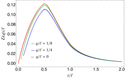
Figure 4: Effect of gain and loss dissipation in the charge-imbalance-resolved negativity ${\cal E}(q)$: ${\cal E}(q)$ is plotted versus $t/\ell$. Here we consider the negativity between two equal adjacent intervals of size $\ell$. The data are for the quench from the Néel state in the tight-binding chain. We consider several values of the charge imbalance $q$. Our results are in the weak-dissipative hydrodynamic limit, i.e., at fixed $t/\ell,q/\ell$ and $\gamma^{+}=1/(2\ell)$ and $\gamma^{-}=1/(4\ell)$, with $\ell=80$ (continuous line) and $\ell=40$ (solid line).

To compute the charge-imbalance-resolved negativity, let us first consider the charged negativity ${\cal E}(\alpha)$ as

$${\cal E}(\alpha)=\lim_{r\to 1}\log(N_{r}(\alpha)),\quad\mathrm{with}\,\,r\,\,\mathrm{even},$$ (86)

where $N_{r}(\alpha)$ is defined in (42). The strategy, again, is to employ the results of [86]. Unlike the case in (84), to evaluate $\log(N_{r}(\alpha))$ one has to obtain the behaviour of $\Gamma_{\mathrm{x}}^{r}$ (cf. (44)) for arbitrary $r$. These terms, however, can be obtained by using the results of Ref. [86]. The calculation is cumbersome and, since it is similar to Ref. [86], we do not report it. For even $r$, the result reads as

$$\mathcal{E}_{r}(\alpha)=-i\alpha\ell+\frac{\ell}{2}\displaystyle\int_{-\pi}^{\pi}\frac{dk}{2\pi}\Big{\{}2h_{\frac{r}{2},\alpha}\left(\frac{1}{2}\pm\frac{1-a}{1+(1-a)^{2}}\right)+\\ \Theta_{1}\Big{[}h_{\frac{r}{2},\alpha}\left(\frac{1}{2}\pm\frac{1-a-b}{1+(1-a-b)^{2}}\right)+\big{(}b\to-b\big{)}-2h_{\frac{r}{2},\alpha}\left(\frac{1}{2}\pm\frac{1-a}{1+(1-a)^{2}}\right)\Big{]}+\\ \Theta_{2}\left[h_{\frac{r}{2},\alpha}\left(\frac{1}{2}\pm\frac{1-a}{[1+(1-a-b)^{2}]^{1/2}[1+(1-a+b)^{2}]^{1/2}}\right)-h_{\frac{r}{2},\alpha}\left(\frac{1}{2}\pm\frac{1-a}{1+(1-a)^{2}}\right)\right]\Big{\}}\\ +r\ell\displaystyle\int_{-\pi}^{\pi}\frac{dk}{2\pi}\Big{\{}\left[2h_{2,0}\left(\frac{a}{2}\right)-h_{2,0}\left(\frac{a+b}{2}\right)-h_{2,0}\left(\frac{a-b}{2}\right)\right]\Theta_{3}\\ +\left[h_{2,0}\left(\frac{a+b}{2}\right)+h_{2,0}\left(\frac{a-b}{2}\right)\right]\Big{\}},$$ (87)

where one has to sum over the $\pm$ signs. The functions $a$ and $b$ are the same as in (81). In (87) the function $h_{r,\alpha}$ is the same as in (78), whereas $\Theta_{1}$ and $\Theta_{2}$ are defined in (82) and (83). In (87) we defined the new function $\Theta_{3}$ as

$$\Theta_{3}=2\mathrm{min}(1/2,|v(k)|t/\ell)-2\mathrm{min}(0,1/2+d/(2\ell)-|v(k)|t/\ell)\\ +\mathrm{min}(0,1+d/(2\ell)-|v(k)|t/\ell)+\mathrm{min}(0,d/(2\ell)-|v(k)|t/\ell).$$ (88)

Now, the first integral in (87) originates from the contribution of $\Gamma_{\mathrm{x}}$ (see the first term in (46)), whereas the second one is due to the second term in (46). Notice that $\Theta_{3}$ is the same function describing the dynamics of the entropies of $A_{1}\cup A_{2}$ (see Fig. 1).

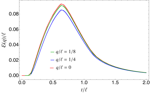
Figure 5: Same as in Fig. 4 for two disjoint intervals at $d=\ell/4$.

The charged negativity is obtained by setting $r=1$ in (87).

From the expression for the charged negativity ${\cal E}_{r}(\alpha)$ (cf. (87)) we obtain the charge-imbalance-resolved negativity by first deriving the moments of the TR partial transpose ${\mathcal{Z}}_{R_{1},r_{e}}(q)$ via the Fourier transform in (37). This step has to be performed numerically. Finally, the charge-imbalance-resolved negativity ${\cal E}(q)$ is obtained from (38).

Our theoretical results for ${\cal E}(q)$ are shown in Fig. 4 and Fig. 5 for two equal-length adjacent and disjoint intervals, respectively. For two adjacent intervals we plot the density of negativity ${\cal E}(q)/\ell$ versus $t/\ell$. Our results hold in the weak-dissipative hydrodynamic limit. This corresponds to the usual hydrodynamic limit $t,\ell\to\infty$ with their ratio $t/\ell$ fixed. We also consider the limit $q\to\infty$ with fixed $q/\ell$. Finally, we consider the weak dissipation limit $\gamma^{\pm}\to 0$ with fixed $\gamma^{\pm}\ell$. The charge-imbalance-resolved negativity exhibits a typical “rise and fall” dynamics. This behaviour is observed also in the absence of dissipation [86]. However, the short-time dynamics is not linear, in contrast with the non dissipative case. For each value of $q/\ell$ in Fig. 4 we show results for $\ell=40$ and $\ell=80$ (continuous and dashed line, respectively). The dependence on $\ell$, which could arise because of the Fourier tranform, is quite weak. Finally, we observe that at very short times ${\cal E}(q)$ suffers from numerical instability in the evaluation of the Fourier transform for this geometry, therefore we do not show the plot for short times. While it is likely that the presence of generic dissipation suppresses the time delay, as it happens for the entropies, clarifying this issue would require considerable numerical effort, and we leave it as an open problem. In Fig. 5 we consider two disjoint intervals at distance $d=\ell/4$. The behaviour of ${\cal E}(q)$ is similar to the case of adjacent intervals, the only difference being that now the negativity is zero up to $t\lesssim d/(2v_{\mathrm{max}})$, with $v_{\mathrm{max}}$ the maximum velocity in the system.

7 Numerical benchmarks

In this section we provide numerical benchmarks for the results derived in sections 5 and 6. Precisely, in section 7.1 we discuss the charged moments, and in section 7.2 and section 7.3 we focus on the symmetry-resolved entropy. In section 7.4 we investigate the weak dissipative limit and logarithmic scaling corrections. In section 7.5 we consider the charge-imbalance-resolved negativity.

7.1 Charged moments

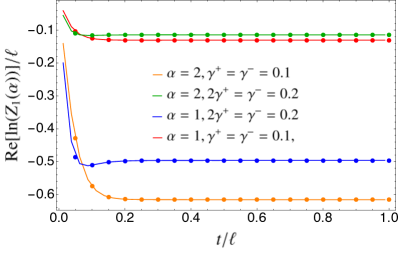
Figure 6: Effect of gain/loss dissipation in the tight-binding chain after the quench from the fermionic Néel state: Real part of the logarithm of the charged moments $\mathrm{Re}[\log(Z_{r}(\alpha))]/\ell$ plotted versus $t/\ell$. We show results for $r=1$ and $r=2$ in the left and right panel, respectively. The symbols are exact lattice data for several values of $\alpha$ and gain/loss rates $\gamma^{\pm}$. The data are for fixed $\ell=80$. The continuous lines are the quasiparticle predictions (cf. (50)).

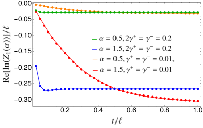
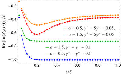
Figure 7: Same as in Fig. 6 for the quench from the Majumdar-Ghosh state.

Let us start discussing the hydrodynamic limit of the charged moments $Z_{r}(\alpha)$ (cf. (27) for their definitions in the lattice model). We report numerical results for the charged moments in Fig. 6 and Fig. 7 for the quench from the Néel state and the Majumdar-Ghosh state, respectively. In the figures we show $\log(Z_{r}(\alpha))/\ell$ plotted versus $t/\ell$. The results are for a finite interval of length $\ell$ embedded in the infinite chain. We show results for several values of the gain/loss rates $\gamma^{\pm}$ (symbols in the figure). Importantly, although we are interested in the weak-dissipative limit in which $\gamma^{\pm}\to 0$ with $\gamma^{\pm}\ell$ fixed, here we show results for finite $\gamma^{\pm}$. The continuous lines in the figures is the theoretical prediction (50). Notice that at $t=0$ one has that

$$\left.\log(Z_{r}(\alpha))\right|_{t=0}=\ell\int_{-\pi}^{\pi}\frac{dk}{2\pi}h^{\mathrm{mix}}_{r}(\alpha).$$ (89)

On the other hand, in the limit $t\to\infty$, one has that (50) reduces to

$$\left.\log(Z_{r}(\alpha))\right|_{t\to\infty}=\ell\int_{-\pi}^{\pi}\frac{dk}{2\pi}h^{\mathrm{q}}_{r}(\alpha).$$ (90)

We should stress that since both $h^{\mathrm{mix}}_{r}(\alpha)$ and $h^{\mathrm{q}}_{r}(\alpha)$ depend on time, one has to take the limits $t=0$ and $t\to\infty$ also within the integrand in (89) and (90). Now, as it is clear from Fig. 6 and Fig. 7, the agreement between the numerical data (symbols in the figures) and the quasiparticle picture is perfect, even away from the weak dissipation limit.

7.2 Symmetry-resolved entropies

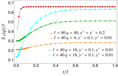
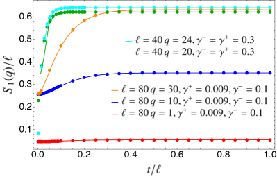
Figure 8: Dynamics of the symmetry-resolved entanglement entropy $S_{1}(q)$ in the tight-binding chain after the Néel (left) and dimer quench (right). We show results for several values of $q$, interval size $\ell$, and dissipation rates $\gamma^{\pm}$. The symbols are the lattice results. The solid line is obtained by computing numerically Eq. (26) as Fourier transform of the quasiparticle prediction (50). The dashed line in the left panel is the quadratic approximation (cf. (70)).

Having confirmed our theoretical results for the charged moments (50), we now consider the symmetry-resolved von Neumann entropy. As discussed in section 5.2, the strategy is to plug the quasiparticle prediction (50) for the charged moments $Z_{r}(\alpha)$ in (25), then performing the Fourier transform numerically. In Fig. 8 we compare our analytic prediction against exact numerical data for the symmetry-resolved entropy. We show results for both the quench from the Néel state and the Majumdar-Ghosh state (left and right panel, respectively). We stress that the fact that the symmetry-resolved entropies are non-vanishing for $t>0$ for any charge sector is due to the presence of dissipative terms: They suppress the delay and all the charge sectors are populated as soon as the state evolves, in contrast with what happens without dissipation [69] or in the presence of pure loss/gain.

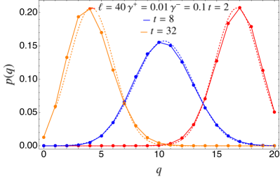
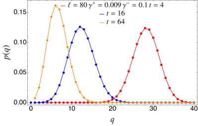
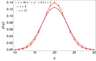
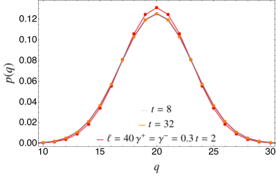
Figure 9: Charge probability distribution of the tight-binding chain after the Néel (left) or dimer quench (right) as a function of $q$ for fixed values of $\ell,t\gamma_{\pm}$. The solid line is obtained by performing numerically the integral in Eq. (25) as Fourier transform of the quasiparticle prediction (50), while the dashed line for the Néel quench is obtained from the quadratic approximation (cf. Eq. (73)).

7.3 Quadratic approximation

Let us now discuss the regime of validity of the quadratic approximation discussed in section 5.2. This is obtained by expanding the charged moments $Z_{r}(\alpha)$ (cf. (27)) around $\alpha=0$. Then, one can perform the Fourier transform in (25) analytically. The result is reported in Fig. 8 (left) as dashed lines. Interestingly, the quadratic approximation works well for the case of balanced gain and loss dissipation, i.e., for $\gamma^{+}=\gamma^{-}$. However, away from the case of balanced dissipation the quadratic approximation fails to describe the dynamics of the entropy.

The reason of this failure is understood by monitoring the behaviour of the charge probability distribution $p(q)=\mathcal{Z}_{1}(q)$. We show results for $p(q)$ in Fig. 9. The left and right panels in the figure are for the quench for the Néel and the Majumdar-Ghosh state, respectively, while top and bottom panels show results for $\gamma^{+}\ll\gamma^{-}$ and $\gamma^{-}=\gamma^{+}$. As we can notice from the figure, the evolution of $p(q)$ is affected by the gain/loss terms. The main difference is that while for $\gamma^{-}=\gamma^{+}$ (i.e. $n_{\infty}=1/2$), $p(q)$ remains peaked around $q=\ell/2$, for $\gamma^{+}\ll\gamma^{-}$, since $n_{\infty}\ll 1$ (cf. (17)), as $t$ increases, the peak of $p(q)$ moves toward smaller and smaller values of $q$. Hence, since the symmetry resolved entropies in Fig.  8 are for fixed value of $q$, for $\gamma^{+}\ll\gamma^{-}$ we have that $\Delta q=q-\bar{q}$ drifts as time passes to larger and larger values because of the drift of $\bar{q}$. Now the quadratic approximation is valid only in the neighbourhood of $\Delta q=0$ (i.e. for $\Delta q\ll\mathcal{B}^{(2)}_{r}$). Working at fixed $q$, such condition breaks down unless $\gamma^{-}=\gamma^{+}$, for which $\bar{q}$ stays constant. This observation physically explains the failure of the quadratic approximation observed in Fig. 8. Moreover, from Fig. 8 it is clear that, for $\gamma_{+}=0.01,\gamma_{-}=0.1$, there is only a tiny time window (corresponding to $\Delta q\simeq 0$) where the quadratic approximation is valid.

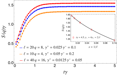
Figure 10: Symmetry-resolved entanglement entropy for the tight-binding chain after the Néel quench in the presence of gain and loss dissipation. Weak-dissipative hydrodynamic scaling limit. We plot $S(q)\gamma$ versus the rescaled time $t\gamma$, with $\gamma=\gamma^{+}+\gamma^{-}$. To reach the scaling limit we rescale also the dissipation rates as $\gamma^{+}=1/(2\ell)$, $\gamma^{-}=2/\ell$. Moreover, we fix $q/\ell=2/5$. Sizeable corrections are visible and prevent from observing a data collapse. In the inset we show data at fixed $t/\ell=1.8$ as a function of $1/\ell$. The continuous line is a fit to $A-1/2\gamma\log(\ell)+B/\ell$, with $A,B$ fitting parameters.

7.4 Logarithmic scaling corrections and the number entropy

It is important to investigate explicitly the scaling behaviour in the weak-dissipative hydrodynamic limit. This is discussed in Fig. 10. We plot exact numerical data for the symmetry-resolved von Neumann entropy for $\ell,t\to\infty$ at fixed $t/\ell$ and $\gamma^{\pm}\to 0$ with fixed $\gamma^{\pm}\ell$. Moreover, we also fix $q/\ell$. Clearly, Fig. 10 shows that there are strong finite $\ell$ corrections. Indeed, in the weak-dissipative hydrodynamic limit all the data in Fig. 10 are expected to collapse on the same curve. Deviations from the expected behaviour can be attributed to the presence of logarithmic terms in $S(q)$. This is due to the fact that the result for the symmetry-resolved entropies should behave like (for $t\to\infty$)

$$S_{1}(q)=a\ell-\frac{1}{2}\log\ell+O(1/\ell).$$ (91)

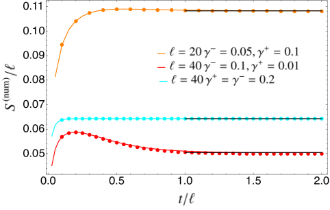
Figure 11: Dynamics of the number entropy (cf. (22)) $S^{(\mathrm{num})}$ after the quench from the Néel state in the tight-binding chain with gain/loss dissipation. The symbols denote exact lattice results, whereas the solid line is the prediction of the quasiparticle picture (cf. (75)). The horizontal line is the result in the long time limit (76).

The logarithmic correction in (91) is captured already by the quadratic approximation (cf. (71)). In the sum rule (22), this logarithmic term cancels with the number entropy and so it can be better understood by studying the latter which is shown in Fig. 11. The figure shows that at $t=0$ the number entropy is zero, reflecting that the initial state is a product state. At later times the entropy grows, and it exhibits an exponential saturation at long times. The symbols in the figures are exact numerical data for $S^{(\mathrm{num})}$, whereas the continuous line is the analytic result obtained by using the quasiparticle picture. The result is obtained by using (59) (see also (50)), performing the Fourier transform (25) numerically. The predictions of the quasiparticle picture are in perfect agreement with the lattice results, even away from the weak dissipative limit, i.e., for finite $\gamma^{\pm}$. In the figure we also show the long time limit (76) (horizontal line), as obtained from the quadratic approximation, which describes quite well the lattice results.

7.5 Charge-imbalance-resolved negativity

We now numerically investigate the validity of our results for the fermionic negativity (see section 6).

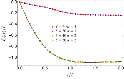
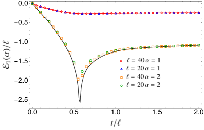
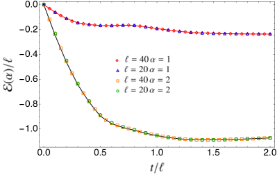
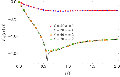
Figure 12: Time evolution of $\mathcal{E}(\alpha)$ (left panels) and $\mathcal{E}_{1}(\alpha)$ (right panels) after a quench from the Néel state in the tight-biding model. The top and bottom panels are for two adjacent and two disjoint intervals at distance $d=\ell/2$, respectively (see Fig. 1). We plot the densities ${\cal E}(\alpha)/\ell$ and ${\cal E}_{1}(\alpha)/\ell$ as a function of $t/\ell$. We fix $\gamma_{+}=1/(2\ell)$, $\gamma_{-}=\gamma_{+}/2$. The data for different $\ell$ at fixed $\alpha$ collapse on the same curve, which is in perfect agreement with (87) (left panels), and (84) (right panels).

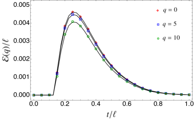
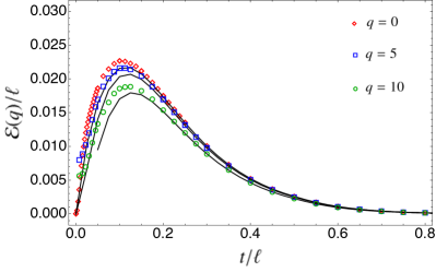
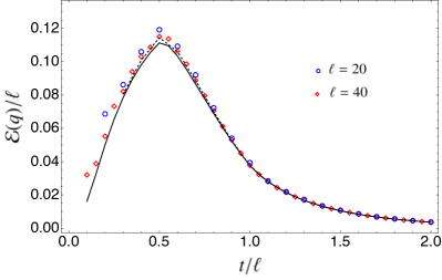
Figure 13: Top panel: Time evolution of ${\mathcal{E}}(q)$ after a quench from the Néel state in the tight-binding model as a function of $t/\ell$ with $\ell=40$, $d=\ell/4$ (left), $d=0$ (right) with fixed $\gamma_{-}=0.1$, $\gamma_{+}=0.01$. Bottom panel: weak dissipative hydrodynamic limit. ${\cal E}(q)$ for $\ell=20,40$, for $d=0$, $\gamma_{+}=1/(2\ell)$, $\gamma_{-}=\gamma_{+}/2$, and $q/\ell=1/4$.

First, we consider the charged negativity ${\cal E}(\alpha)$ defined in (86). In Fig. 12 we show exact numerical data for ${\cal E}_{1}(\alpha)$ and ${\cal E}(\alpha)$ (left and right panels, respectively) in the tight-binding chain with gain and loss of fermions. We consider the quench from the fermionic Néel state. Since we are interested in the weak-dissipative hydrodynamic limit, we plot ${\cal E}(\alpha)/\ell$ versus $t/\ell$. To reach the weak-dissipation limit we rescale the dissipation rates $\gamma^{\pm}$ as $1/\ell$. Specifically, we choose $\gamma^{+}=1/(2\ell)$ and $\gamma^{-}=\gamma^{+}/2$. We show results for several values of $\alpha$. The top panels are for two adjacent intervals, whereas the bottom ones are for two disjoint ones at $d=\ell/2$. Our theoretical predictions are (84) and (87). Now, the symbols in Fig. 12 are exact numerical data for ${\cal E}(\alpha)$ and ${\cal E}_{1}(\alpha)$. Our theoretical predictions are shown as continuous lines in the figure, and are in perfect agreement with the numerical data.

Finally, we discuss the charge-imbalance-resolved negativity ${\mathcal{E}}(q)$. This is obtained by using (84) and (87) in (37), performing the Fourier transform numerically, and using (38). We show numerical results in Fig. 13. The top panels in the figure are for fixed $\gamma^{-}=0.1$ and $\gamma^{+}=0.01$, $\ell=40$ and $q=0,5,10$. The top-right panel shows results for two adjacent intervals, i.e., for $d=0$, whereas the top-left one is for two disjoint intervals at $d=\ell/2$. The continuous lines in the figures are the theoretical results obtained from the quasiparticle picture. The agreement between lattice results and hydrodynamic limit is perfect for two disjoint intervals. Deviations from the scaling limit are visible for two adjacent intervals (top-right panel in Fig. 13). These are due to the fact that our results are valid only in the weak-dissipative hydrodynamic limit. Similar corrections are observed in the absence of dissipation [87]. The right plot also clearly shows that there is no delay in the presence of dissipation, since $\mathcal{E}(q)$ is different from zero as soon as $t>0$, at least for $q=0,5$. The scaling behaviour for two adjacent intervals is better investigated in Fig. 13 in the bottom panel. We now show results in the limit $\ell,t,q\to\infty$ with $t/\ell,q/\ell$ fixed. Moreover, we consider $\gamma^{\pm}\to 0$ at fixed $\gamma^{\pm}\ell$. Now, although for finite $\ell$ some deviations are present, upon increasing $\ell$ the numerical results approach the analytic predictions (lines in the figure).

8 Conclusions

We investigated the effects of gain and loss dissipation in the dynamics of the symmetry-resolved entropies and charge-imbalance-resolved negativity after a quantum quench in the tight-binding chain. This choice of dissipative terms preserves the block-diagonal structure of the reduced density matrix, and it is therefore suitable to study the symmetry resolution of entanglement in each charge sector. We derived quasiparticle picture formulas for the dynamics of charged moments of the reduced density matrix, the symmetry-resolved von Neumann entropy, and the charge-imbalance-resolved negativity. Our results hold in the hydrodynamic limit of large intervals and long times, with their ratio fixed. Moreover, to ensure a nontrivial scaling behaviour we also considered weak dissipation. We showed that while the symmetry-resolved entropies are dominated by dissipative processes, the resolved negativity exhibits the typical rise and fall dynamics, reflecting that it is sensitive to entangled quasiparticles. Furthermore, we observed that the entropy does not exhibit a time delay (unless we consider a pure gain/loss evolution), contrarily to what happens in the non-dissipative case.

Let us now mention some possible directions for future research. First, it would be interesting to extend our results to other types of dissipation, for instance, for generic quadratic Lindblad master equations [84, 85]. While this is feasible for the symmetry-resolved entropies, it is a challenging task for the negativity. Indeed, even for the non-resolved negativity only the case of free fermions with gain and loss dissipation was investigated so far [86]. Clearly, it would be important to go beyond the case of quadratic Lindblad equations, considering more complicated dissipators, such as dephasing [107]. For instance, it would be interesting to employ recent results obtained for this dissipator in Ref. [108]. Finally, one could study the effects of dissipative terms which do not preserve the block-diagonal structure of the reduced density matrix and quantify how much the symmetry is broken in this setup by using the entanglement asymmetry studied in [73, 75]. Similarly, one could consider initial states that explicitly breaks the internal symmetry and study the evolution of the asymmetry subject to gain and loss.

References

- [1] A. Polkovnikov, K. Sengupta, A. Silva and M. Vengalattore, Nonequilibrium dynamics of closed interacting quantum systems, Rev. Mod. Phys. 83, 863 (2011).
- [2] C. Gogolin and J. Eisert, Equilibration, thermalisation, and the emergence of statistical mechanics in closed quantum systems, Rep. Progr. Phys. 79, 056001 (2016).
- [3] L. D’Alessio, Y. Kafri, A. Polkovnikov and M. Rigol, From quantum chaos and eigenstate thermalization to statistical mechanics and thermodynamics, Adv. Phys. 65, 239 (2016).
- [4] P. Calabrese, F. H. L. Essler and G. Mussardo, Introduction to ‘Quantum Integrability in Out of Equilibrium Systems’, J. Stat. Mech. 064001 (2016).
- [5] F. H. L. Essler and M. Fagotti, Quench dynamics and relaxation in isolated integrable quantum spin chains, J. Stat. Mech. 064002 (2016).
- [6] P. Calabrese and J. Cardy, Evolution of entanglement entropy in one-dimensional systems, J. Stat. Mech. P04010 (2005).
- [7] M. Fagotti and. Calabrese, Evolution of entanglement entropy following a quantum quench: Analytic results for the XY chain in a transverse magnetic field, Phys. Rev. A 78, 010306 (2008).
- [8] V. Alba and P. Calabrese, Entanglement and thermodynamics after a quantum quench in integrable systems, PNAS 114, 7947 (2017).
- [9] V. Alba and P. Calabrese, Entanglement dynamics after quantum quenches in generic integrable systems SciPost Phys. 4, 17 (2018).
- [10] V. Alba and P. Calabrese, Quench action and Rényi entropies in integrable systems, Phys. Rev. B 96, 115421 (2017).
- [11] B. Bertini, K. Klobas, V. Alba, G. Lagnese and P. Calabrese, Growth of Rényi Entropies in Interacting Integrable Models and the Breakdown of the Quasiparticle Picture, Phys. Rev. X 12, 031016 (2022).
- [12] P. Calabrese, Entanglement spreading in non-equilibrium integrable systems, SciPost Phys. Lect. Notes 20 (2020).
- [13] A. M. Kaufman, M. E. Tai, A. Lukin, M. Rispoli, R. Schittko, P. M. Preiss and M. Greiner, Quantum thermalization through entanglement in an isolated many-body system, Science 353, 794 (2016).
- [14] A. Lukin, M. Rispoli, R. Schittko, M. E. Tai, A. M. Kaufman, S. Choi, V. Khemani, J. Léonard and M. Greiner, Probing entanglement in a many-body localized system, Science 364, 256 (2019).
- [15] T. Brydges, A. Elben, P. Jurcevic, B. Vermersch, C. Maier, B. P. Lanyon, P. Zoller, R. Blatt and C. F. Roos, Probing Rényi entanglement entropy via randomized measurements, Science 364, 260 (2019).
- [16] A. Elben, R. Kueng, H. Y. R. Huang, R. van Bijnen, C. Kokail, M. Dalmonte, P. Calabrese, B. Kraus, J. Preskill, P. Zoller and B. Vermersch, Mixed-State Entanglement from Local Randomized Measurements, Phys. Rev. Lett. 125, 200501 (2020).
- [17] N. Laflorencie and S. Rachel, Spin-resolved entanglement spectroscopy of critical spin chains and Luttinger liquids, J. Stat. Mech. (2014) P11013.
- [18] M. Goldstein and E. Sela, Symmetry-Resolved Entanglement in Many-Body Systems, Phys. Rev. Lett. 120, 200602 (2018).
- [19] J. C. Xavier, F. C. Alcaraz, and G. Sierra, Equipartition of the entanglement entropy, Phys. Rev. B 98, 041106 (2018).
- [20] A. Neven, J. Carrasco, V. Vitale, C. Kokail, A. Elben, M. Dalmonte, P. Calabrese, P. Zoller, B. Vermersch, R. Kueng, and B. Kraus, Symmetry-resolved entanglement detection using partial transpose moments, Npj Quantum Inf. 7, 152 (2021).
- [21] V. Vitale, A. Elben, R. Kueng, A. Neven, J. Carrasco, B. Kraus, P. Zoller, P. Calabrese, B. Vermersch, and M. Dalmonte, Symmetry-resolved dynamical purification in synthetic quantum matter, SciPost Phys. 12, 106 (2022).
- [22] A. Rath, V. Vitale, S. Murciano, M. Votto, J. Dubail, R. Kueng, C. Branciard, P. Calabrese, and B. Vermersch, Entanglement barrier and its symmetry resolution: theory and experiment, PRX Quantum 4, 010318 (2023).
- [23] S. Murciano, G. Di Giulio, and P. Calabrese, Entanglement and symmetry resolution in two dimensional free quantum field theories, JHEP 08 (2020) 073.
- [24] D. X. Horvath and P. Calabrese, Symmetry resolved entanglement in integrable field theories via form factor bootstrap, JHEP 11 (2020) 131.
- [25] D. X. Horvath, L. Capizzi, and P. Calabrese, U(1) symmetry resolved entanglement in free 1+1 dimensional field theories via form factor bootstrap, JHEP 05 (2021) 197.
- [26] D. X. Horvath, P. Calabrese, and O. A. Castro-Alvaredo, Branch Point Twist Field Form Factors in the sine-Gordon Model II: Composite Twist Fields and Symmetry Resolved Entanglement, SciPost Phys. 12, 088 (2022).
- [27] L. Capizzi, D. X. Horvath, P. Calabrese, and O. A. Castro-Alvaredo, Entanglement of the 3-State Potts Model via Form Factor Bootstrap: Total and Symmetry Resolved Entropies, JHEP 05 (2022) 113.
- [28] L. Capizzi, O. A. Castro-Alvaredo, C. De Fazio, M. Mazzoni, and L. Santamaria-Sanz, Symmetry Resolved Entanglement of Excited States in Quantum Field Theory I: Free Theories, Twist Fields and Qubits, JHEP 12 (2022) 127.
- [29] L. Capizzi, O. A. Castro-Alvaredo, C. De Fazio, M. Mazzoni, and L. Santamaria-Sanz, Symmetry Resolved Entanglement of Excited States in Quantum Field Theory II: Numerics, Interacting Theories and Higher Dimensions, JHEP 12 (2022) 128.
- [30] L. Capizzi, M. Mazzoni, and O. A. Castro-Alvaredo Symmetry Resolved Entanglement of Excited States in Quantum Field Theory III: Bosonic and Fermionic Negativity, arXiv:2302.02666.
- [31] M. Mazzoni and O. A. Castro-Alvaredo, Two-Point Functions of Composite Twist Fields in the Ising Field Theory, arXiv:2301.01745.
- [32] L. Capizzi and P. Calabrese, Symmetry resolved relative entropies and distances in conformal field theory, JHEP 10 (2021) 195.
- [33] L. Hung and G. Wong, Entanglement branes and factorization in conformal field theory, Phys. Rev. D 104, 026012 (2021).
- [34] P. Calabrese, J. Dubail, and S. Murciano, Symmetry-resolved entanglement entropy in Wess-Zumino-Witten models, JHEP 10 (2021) 067.
- [35] A. Milekhin and A. Tajdini, Charge fluctuation entropy of Hawking radiation: a replica-free way to find large entropy, arXiv:2109.03841.
- [36] M. Ghasemi, Universal Thermal Corrections to Symmetry-Resolved Entanglement Entropy and Full Counting Statistics, arXiv:2203.06708.
- [37] B. Estienne, Y. Ikhlef, and A. Morin-Duchesne, Finite-size corrections in critical symmetry-resolved entanglement, SciPost Phys. 10, 054 (2021).
- [38] F. Ares, P. Calabrese, G. Di Giulio, and S. Murciano,, Multi-charged moments of two intervals in conformal field theory, JHEP 09 (2022) 051.
- [39] A. Foligno, S. Murciano, and P. Calabrese, Entanglement resolution of free Dirac fermions on a torus, JHEP 03 (2023) 096.
- [40] G. Di Giulio, R. Meyer, C. Northe, H. Scheppach, and S. Zhao, On the Boundary Conformal Field Theory Approach to Symmetry-Resolved Entanglement, arXiv:2212.09767.
- [41] L. Capizzi, S. Murciano, and P. Calabrese, Full counting statistics and symmetry resolved entanglement for free conformal theories with interface defects, arXiv:2302.08209.
- [42] S. Zhao, C. Northe, and R. Meyer, Symmetry-Resolved Entanglement in AdS3/CFT2 coupled to Chern-Simons Theory, JHEP 07 (2021) 030.
- [43] K. Weisenberger, S. Zhao, C. Northe, and R. Meyer, Symmetry-resolved entanglement for excited states and two entangling intervals in AdS3/CFT2, JHEP 12 (2021) 104.
- [44] S. Zhao, C. Northe, K. Weisenberger, and R. Meyer, Charged Moments in Higher Spin Holography, JHEP 05 (2022) 166.
- [45] S. Baiguera, L. Bianchi, S. Chapman, and D. A. Galante, Shape Deformations of Charged Rényi Entropies from Holography, JHEP 06 (2022) 068.
- [46] R. Bonsignori, P. Ruggiero, and P. Calabrese, symmetry-resolved entanglement in free fermionic systems, J. Phys. A 52, 475302 (2019).
- [47] S. Fraenkel and M. Goldstein, symmetry-resolved entanglement: Exact results in 1d and beyond, J. Stat. Mech. (2020) 033106.
- [48] H. M. Wiseman and J. A. Vaccaro, Entanglement of Indistinguishable Particles Shared between Two Parties, Phys. Rev. Lett. 91, 097902 (2003).
- [49] S. Murciano, G. Di Giulio, and P. Calabrese, Symmetry-resolved entanglement in gapped integrable systems: a corner transfer matrix approach, SciPost Phys. 8, 046 (2020).
- [50] H. Barghathi, C. M. Herdman, and A. Del Maestro, Rényi Generalization of the Accessible Entanglement Entropy, Phys. Rev. Lett. 121, 150501 (2018).
- [51] H. Barghathi, E. Casiano-Diaz, and A. Del Maestro, Operationally accessible entanglement of one dimensional spinless fermions, Phys. Rev. A 100, 022324 (2019).
- [52] H. Barghathi, J. Yu, and A. Del Maestro, Theory of noninteracting fermions and bosons in the canonical ensemble, Phys. Rev. Res. 2, 043206 (2020).
- [53] P. Calabrese, M. Collura, G. Di Giulio, and S. Murciano, Full counting statistics in the gapped XXZ spin chain, EPL 129, 60007 (2020).
- [54] S. Murciano, P. Ruggiero, and P. Calabrese, Symmetry-resolved entanglement in two-dimensional systems via dimensional reduction, J. Stat. Mech. (2020) 083102.
- [55] Z. Ma, C. Han, Y. Meir, and E. Sela, Symmetric inseparability and number entanglement in charge conserving mixed states, Phys. Rev. A 105, 042416 (2022).
- [56] M. T. Tan and S. Ryu, Particle Number Fluctuations, Rényi and Symmetry-resolved Entanglement Entropy in Two-dimensional Fermi Gas from Multi-dimensional bosonisation, Phys. Rev. B 101, 235169 (2020).
- [57] X. Turkeshi, P. Ruggiero, V. Alba, and P. Calabrese, Entanglement equipartition in critical random spin chains, Phys. Rev. B 102, 014455 (2020).
- [58] S. Murciano, P. Calabrese, and L. Piroli, Symmetry-resolved Page curves, Phys. Rev. D 106, 046015 (2022).
- [59] M. Kiefer-Emmanouilidis, R. Unanyan, J. Sirker, and M. Fleischhauer, Bounds on the entanglement entropy by the number entropy in non-interacting fermionic systems, SciPost Phys 8, 083 (2020).
- [60] M. Kiefer-Emmanouilidis, R. Unanyan, J. Sirker, and M. Fleischhauer, Evidence for unbounded growth of the number entropy in many-body localized phases, Phys. Rev. Lett. 124, 243601 (2020).
- [61] M. Kiefer-Emmanouilidis, R. Unanyan, M. Fleischhauer, and J. Sirker, Slow delocalization of particles in many-body localized phases, Phys. Rev. B 103, 024203 (2021).
- [62] M. Kiefer-Emmanouilidis, R. Unanyan, M. Fleischhauer, and J. Sirker, Absence of true localization in many-body localized phases, Phys. Rev. B 103, 024203 (2021).
- [63] Y. Zhao, D. Feng, Y. Hu, S. Guo, and J. Sirker, Entanglement dynamics in the three-dimensional Anderson model, Phys. Rev. B 102, 195132 (2020).
- [64] R. Bonsignori and P. Calabrese, Boundary effects on symmetry-resolved entanglement, J. Phys. A 54, 015005 (2021).
- [65] F. Ares, S. Murciano, and P. Calabrese, Symmetry-resolved entanglement in a long-range free-fermion chain, J. Stat. Mech. (2022) 063104.
- [66] N. G. Jones, Symmetry-resolved entanglement entropy in critical free-fermion chains, J. Stat. Phys. 188, 28 (2022).
- [67] M. Fossati, F. Ares and P. Calabrese, Symmetry-resolved entanglement in critical non-Hermitian systems, arXiv:2303.05232.
- [68] G. Parez, R. Bonsignori, and P. Calabrese, Quasiparticle dynamics of symmetry-resolved entanglement after a quench: the examples of conformal field theories and free fermions, Phys. Rev. B 103, L041104 (2021).
- [69] G. Parez, R. Bonsignori, and P. Calabrese, Exact quench dynamics of symmetry-resolved entanglement in a free fermion chain, J. Stat. Mech. 093102 (2021).
- [70] S. Fraenkel and M. Goldstein, Entanglement Measures in a Nonequilibrium Steady State: Exact Results in One Dimension, SciPost Phys. 11, 085 (2021).
- [71] L. Piroli, E. Vernier, M. Collura, and P. Calabrese, Thermodynamic symmetry-resolved entanglement entropies in integrable systems, J. Stat. Mech. (2022) 073102.
- [72] S. Scopa and D. X. Horvath, Exact hydrodynamic description of symmetry-resolved Rényi entropies after a quantum quench, J. Stat. Mech. (2022) 083104.
- [73] F. Ares, S. Murciano, and P. Calabrese, Entanglement asymmetry as a probe of symmetry breaking, arXiv:2207.14693.
- [74] B. Bertini, P. Calabrese, M. Collura, K. Klobas, and C. Rylands, Nonequilibrium Full Counting Statistics and Symmetry-Resolved Entanglement from Space-Time Duality, arXiv:2212.06188.
- [75] F. Ares, S. Murciano, E. Vernier, and P. Calabrese, Lack of symmetry restoration after a quantum quench: an entanglement asymmetry study, arXiv:2302.03330.
- [76] E. Cornfeld, M. Goldstein, and E. Sela, Imbalance Entanglement: Symmetry Decomposition of Negativity, Phys. Rev. A 98, 032302 (2018).
- [77] S. Murciano, R. Bonsignori, and P. Calabrese, Symmetry decomposition of negativity of massless free fermions, SciPost Phys. 10, 111 (2021).
- [78] H.-H. Chen, Charged Rényi negativity of massless free bosons, JHEP 02 (2022) 117.
- [79] N. Feldman and M. Goldstein, Dynamics of Charge-Resolved Entanglement after a Local Quench, Phys. Rev. B 100, 235146 (2019).
- [80] G. Parez, R. Bonsignori, and P. Calabrese, Dynamics of charge-imbalance-resolved entanglement negativity after a quench in a free-fermion mode, J. Stat. Mech. 053103 (2022).
- [81] H.-H. Chen, Dynamics of charge imbalance resolved negativity after a global quench in free scalar field theory, JHEP 08 (2022) 146.
- [82] H. P. Breuer and F. Petruccione, The theory of open quantum systems, (Great Clarendon Street: Oxford University Press) (2002).
- [83] V. Alba and F. Carollo, Spreading of correlations in Markovian open quantum systems, Phys. Rev. B 103, 020302 (2021).
- [84] F. Carollo and V. Alba, Emergent dissipative quasi-particle picture in noninteracting Markovian open quantum systems, Phys. Rev. B 105, 144305 (2022).
- [85] V. Alba and F. Carollo, Hydrodynamics of quantum entropies in Ising chains with linear dissipation, J. Phys. A: Math. Theor. 55, 074002 (2022).
- [86] V. Alba and F. Carollo, Logarithmic negativity in out-of-equilibrium open free-fermion chains: An exactly solvable case, arXiv:2205.02139 (2022).
- [87] V. Alba and P. Calabrese, Quantum information dynamics in multipartite integrable systems EPL 126, 60001 (2019).
- [88] V. Alba, Unbounded entanglement production via a dissipative impurity, SciPost Phys. 12, 011 (2022).
- [89] F. Caceffo and V. Alba, Entanglement negativity in a fermionic chain with dissipative defects: Exact results, J. Stat. Mech. 023102 (2023).
- [90] A. D’Abbruzzo, V. Alba and D. Rossini, Logarithmic entanglement scaling in dissipative free-fermion systems, Phys. Rev. B 106, 235149 (2022).
- [91] B. Buca and T. Prosen, A note on symmetry reductions of the Lindblad equation: transport in constrained open spin chains, New J. Phys. 14, 073007 (2012).
- [92] L. Sá, P. Ribeiro, and T. Prosen, Symmetry Classification of Many-Body Lindbladians: Tenfold Way and Beyond, arXiv.2212.00474 (2022).
- [93] V. V. Albert and L. Jiang, Symmetries and conserved quantities in Lindblad master equations, Phys. Rev. A 89, 022118 (2014).
- [94] K. Macieszczak and D. C. Rose, Quantum jump Monte Carlo approach simplified: Abelian symmetries, Phys. Rev. A 103, 042204 (2021)
- [95] F. Minganti, I. I. Arkhipov, A. Miranowicz, and F. Nori, Continuous Dissipative Phase Transitions with or without Symmetry Breaking, New J. Phys. 23, 122001 (2021).
- [96] I. Peschel and V. Eisler, Reduced density matrices and entanglement entropy in free lattice models, J. Phys. A 42, 504003 (2009).
- [97] M. Fagotti, On conservation laws, relaxation and pre-relaxation after a quantum quench, J. Stat. Mech. P03016 (2014).
- [98] R. Simon, Peres-Horodecki Separability Criterion for Continuous Variable Systems, Phys. Rev. Lett. 84, 2726 (2000).
- [99] K. Audenaert, J. Eisert, M. B. Plenio, and R. F. Werner, Entanglement properties of the harmonic chain, Phys. Rev. A 66, 042327 (2002)
- [100] V. Eisler and Z. Zimborás, On the partial transpose of fermionic gaussian states, New J. Phys. 117, 053048 (2015).
- [101] A. Coser, E. Tonni, and P. Calabrese, Towards entanglement negativity of two disjoint intervals for a one dimensional free fermion, J. Stat. Mech. 033116 (2016).
- [102] H. Shapourian, K. Shiozaki, and S. Ryu, Partial time-reversal transformation and entanglement negativity in fermionic systems, Phys. Rev. B 95, 165101 (2017).
- [103] H. Shapourian and S. Ryu, Finite-temperature entanglement negativity of free fermions, J. Stat. Mech. 043106 (2019).
- [104] H. Shapourian, P. Ruggiero, S. Ryu, and P. Calabrese, Twisted and untwisted negativity spectrum of free fermions, SciPost Phys. 7, 037 (2019).
- [105] R. Wong, Asymptotic Approximations of Integrals, Society for Industrial and Applied Mathematics, (2001).
- [106] A. Coser, E. Tonni, and P. Calabrese, Entanglement negativity after a global quantum quench, J. Stat. Mech. P12017 (2014).
- [107] D. Wellnitz, G. Preisser, V. Alba, J. Dubail, and J. Schachenmayer, The rise and fall, and slow rise again, of operator entanglement under dephasing, Phys. Rev. Lett. 129, 170401 (2022).
- [108] M. Coppola, G. T. Landi and D. Karevski, Wigner dynamics for quantum gases under inhomogeneous gain and loss processes with dephasing, arxiv:2212.11029 (2022).
- [109] V. Alba and F. Carollo, Noninteracting fermionic systems with localized losses: Exact results in the hydrodynamic limit, Phys. Rev. B, 105 054303 (2022).