Natural Language-Assisted Sign Language Recognition

Abstract

Sign languages are visual languages which convey information by signers’ handshape, facial expression, body movement, and so forth. Due to the inherent restriction of combinations of these visual ingredients, there exist a significant number of visually indistinguishable signs (VISigns) in sign languages, which limits the recognition capacity of vision neural networks. To mitigate the problem, we propose the Natural Language-Assisted Sign Language Recognition (NLA-SLR) framework, which exploits semantic information contained in glosses (sign labels). First, for VISigns with similar semantic meanings, we propose language-aware label smoothing by generating soft labels for each training sign whose smoothing weights are computed from the normalized semantic similarities among the glosses to ease training. Second, for VISigns with distinct semantic meanings, we present an inter-modality mixup technique which blends vision and gloss features to further maximize the separability of different signs under the supervision of blended labels. Besides, we also introduce a novel backbone, video-keypoint network, which not only models both RGB videos and human body keypoints but also derives knowledge from sign videos of different temporal receptive fields. Empirically, our method achieves state-of-the-art performance on three widely-adopted benchmarks: MSASL, WLASL, and NMFs-CSL. Codes are available at https://github.com/FangyunWei/SLRT.

1 Introduction

Sign languages are the primary languages for communication among deaf communities. On the one hand, sign languages have their own linguistic properties as most natural languages [50, 1, 62]. On the other hand, sign languages are visual languages that convey information by the movements of the hands, body, head, mouth, and eyes, making them completely separate and distinct from natural languages [67, 69, 6]. This work dedicates to sign language recognition (SLR), which requires models to classify the isolated signs from videos into a set of glosses. Despite its fundamental capacity of recognizing signs, SLR has a broad range of applications including sign spotting [56, 41, 35], sign video retrieval [10], sign language translation [34, 52, 6], and continuous sign language recognition [6, 1].

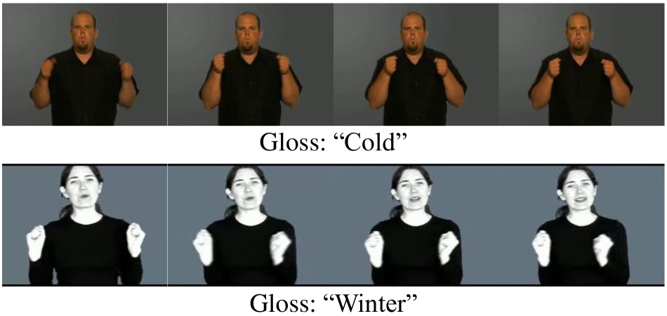
(a) VISigns may have similar semantic meanings.

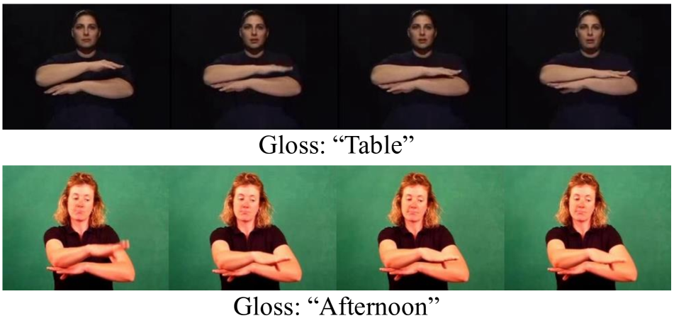
(b) VISigns may have distinct semantic meanings.

Figure 1: Vision neural networks are demonstrated to be less effective to recognize visually indistinguishable signs (VISigns) [2, 33, 25]. We observe that VISigns may have similar or distinct semantic meanings, inspiring us to leverage this characteristic to facilitate sign language recognition as illustrated in Figure 2.

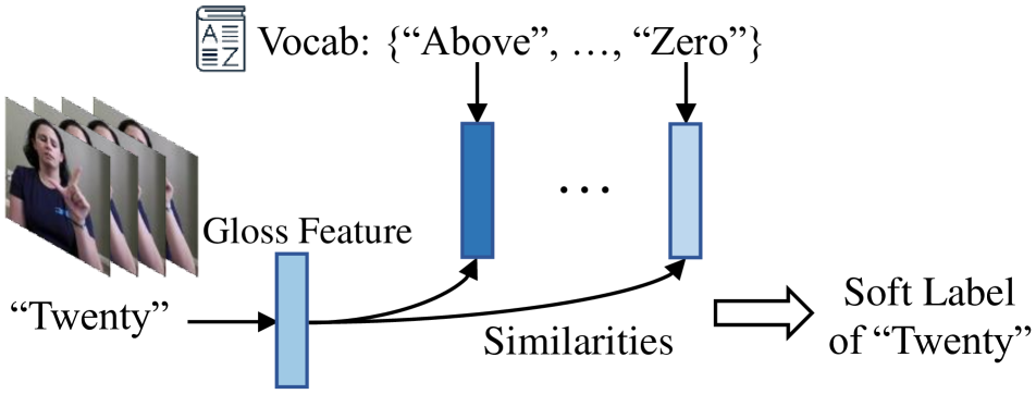
(a) Language-aware label smoothing.

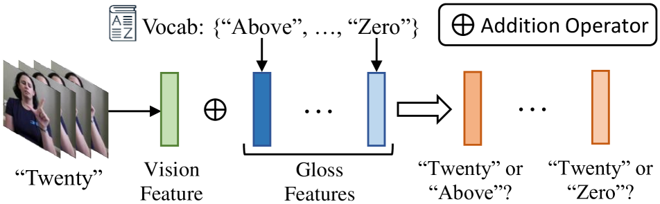
(b) Inter-modality mixup.

Figure 2: We incorporate natural language modeling into sign language recognition to promote recognition capacity. (a) Language-aware label smoothing generates a soft label for each training video, whose smoothing weights are the normalized semantic similarities of the ground truth gloss and the remaining glosses within the sign language vocabulary. (b) Inter-modality mixup yields the blended features (denoted by orange rectangles) with the corresponding mixed labels to maximize the separability of signs in a latent space.

Since the lexical items of sign languages are defined by the handshape, facial expression, and movement, the combinations of these visual ingredients are restricted inherently, yielding plenty of visually indistinguishable signs termed VISigns. VISigns are those signs with similar handshape and motion but varied semantic meanings. We show two examples (“Cold” vs. “Winter” and “Table” vs. “Afternoon”) in Figure 1. Unfortunately, vision neural networks are demonstrated to be less effective to accurately recognize the VISigns [2, 33, 25]. Due to the intrinsic connections between sign languages and natural languages, the glosses, i.e., labels of signs, are semantically meaningful in contrast to the one-hot labels used in traditional classification tasks [26, 49]. Thus, although the VISigns are challenging to be classified from the vision perspective, their glosses provide serviceable semantics, which is, however, less taken into consideration in previous works [18, 17, 19, 35, 33, 25, 23, 22]. Our work is built upon the following two findings.

Finding-1: VISigns may have similar semantic meanings (Figure 1(a)). Due to the observation that VISigns may have higher visual similarities, assigning hard labels to them may hinder the training since it is challenging for vision neural networks to distinguish each VISign apart. A straightforward way to ease the training is to replace the hard labels with soft ones as in well-established label smoothing [54, 14]. However, how to generate proper soft labels is non-trivial. The vanilla label smoothing [54, 14] assigns equal smoothing weights to all negative terms, which ignores the semantic information contained in labels. In light of the finding-1 that VISigns may have similar semantic meanings and the intrinsic connections between sign languages and natural languages, we consider the semantic similarities among the glosses when generating soft labels. Concretely, for each training video, we adopt an off-the-shelf word representation framework, i.e., fastText [38], to pre-compute the semantic similarities of its gloss and the remaining glosses within the sign language vocabulary. Then we can properly generate a soft label for each training sample whose smoothing weights are the normalized semantic similarities. In this way, negative terms with similar semantic meanings to the ground truth gloss are assigned higher values in the soft label. As shown in Figure 2(a), we term this process as language-aware label smoothing, which injects prior knowledge into the training.

Finding-2: VISigns may have distinct semantic meanings (Figure 1(b)). Although the VISigns are challenging to be classified from the vision perspective, the semantic meanings of their glosses may be distinguishable according to finding-2. This inspires us to combine the vision features and gloss features to drive the model towards maximizing signs’ separability in a latent space. Specifically, given a sign video, we first leverage our proposed backbone to encode its vision feature and the well-established fastText [38] to extract the feature of each gloss within the sign language vocabulary. Then we independently integrate the vision feature and each gloss feature to produce a blended representation, which is further fed into a classifier to approximate its mixed label. We refer to this procedure as inter-modality mixup as shown in Figure 2(b). We empirically find that our inter-modality mixup significantly enhances the model’s discriminative power.

Our contributions can be summarized as follows:

• We are the first to incorporate natural language modeling into sign language recognition based on the discovery of VISigns. Language-aware label smoothing and inter-modality mixup are proposed to take full advantage of the linguistic properties of VISigns and semantic information contained in glosses.

• We take into account the unique characteristic of sign languages and present a novel backbone named video-keypoint network (VKNet), which not only models both RGB videos and human keypoints, but also derives knowledge from sign videos of various temporal receptive fields.

• Our method, termed natural language-assisted sign language recognition (NLA-SLR), achieves state-of-the-art performance on the widely-used SLR datasets including MSASL [25], WLASL [33], and NMFs-CSL [19].

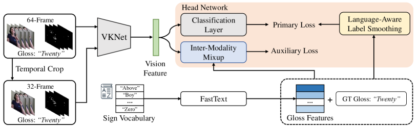
Figure 3: An overview of our NLA-SLR. Given a training video, we temporally crop a 64-frame clip [35] and use HRNet [53] trained on COCO-WholeBody [24] to estimate its keypoint sequence which is represented by a set of heatmaps, yielding a 64-frame video-keypoint pair. Then we temporally crop a 32-frame counterpart and feed it along with the 64-frame pair into our proposed VKNet (Figure 4) to extract the vision feature. The head network (Figure 5) has a two-branch architecture consisting of a language-aware label smoothing branch and an inter-modality mixup branch. We only retain the VKNet and the classification layer in the head network for inference.

2 Related Works

Sign Language Recognition. Sign language recognition (SLR) is a fundamental task in the field of sign language understanding. Feature extraction plays a key role in an SLR model. Most recent SLR works [22, 23, 17, 18, 35, 33, 25, 19, 67, 70, 39] adopt CNN-based architectures, e.g., I3D [4] and R3D [44], to extract vision features from RGB videos. In this work, we adopt S3D [57] as the backbone of our VKNet due to its excellent accuracy-speed trade-off.

However, RGB-based SLR models may suffer from the large variation of video backgrounds. As a complement, some SLR works [23, 22, 18, 17, 7] explore to jointly model RGB videos and keypoints. For example, SAM-SLR [23] uses graph convolutional networks (GCNs) to model pre-extracted keypoints. HMA [18] and SignBERT [17] propose to decode 3D hand keypoints from RGB videos. A common deficiency of these works is that they need a dedicated network to model keypoints. In this work, we represent keypoints as a sequence of heatmaps [9, 7] so that the keypoint encoder of our VKNet can share the identical architecture with the video encoder.

To enable mini-batch training, previous works [22, 23, 17, 18, 35, 33] crop fixed-length clips from raw videos as model inputs. However, the model may overfit to the training videos of fixed temporal receptive fields. In contrast, our VKNet is trained on videos with varied temporal receptive fields to improve its generalization capability.

Word Representation Learning. Word2vec [37] and GloVe [43] are two classical word representation learning frameworks in the field of NLP. Based on word2vec, fastText [38] improves word representations with several modifications including the use of sub-word information [3] and position independent features [40]. Although some advanced language models, e.g., BERT [28], can also be used to extract word representations, they are computationally intensive and are not dedicated to word representation learning. In this paper, we adopt the lightweight but effective fastText, which is also used in a recent sign language translation work [63], to pre-compute gloss (word) representations.

Vision-Language Models. Recently, a majority of vision-language models [45, 21, 61, 13] learn visual representations on large-scale image-text pairs. Among them, CLIP [45] is the pioneer to jointly optimize an image encoder and a text encoder through a contrastive loss. Besides, the pre-trained CLIP can be generalized to various downstream tasks, e.g., semantic segmentation [58, 32, 59], object detection [8, 47], image classification [68, 20], and style transfer [42, 31]. In this work, we exploit the implicit knowledge included in glosses (sign labels), which is distinct from previous works on vision-language modeling.

Multi-label Classification. Real-world objects may have multiple semantic meanings, which motivates research on multi-label classification [48, 27, 65, 46, 29] requiring models to map inputs to multiple possible labels. Although the VISigns may be associated with the multi-label classification problem, most widely-adopted SLR datasets [33, 25, 19] are singly labeled. In this work, we deal with the VISigns by incorporating language information included in glosses.

3 Methodology

An overview of our natural language-assisted sign language recognition (NLA-SLR) framework is shown in Figure 3. Our framework mainly consists of three parts: 1) data pre-processing which generates video-keypoint pairs as network inputs (Section 3.1); 2) a video-keypoint network (VKNet) which takes video-keypoint pairs of various temporal receptive fields as inputs for vision feature extraction (Section 3.2); 3) a head network (Section 3.3) containing a language-aware label smoothing branch (Section 3.3.1) and an inter-modality mixup branch (Section 3.3.2). We empirically find that Mixup [64] can be applied on both RGB videos and keypoint heatmap sequences, which will be described in Section 3.4.

3.1 Data Pre-Processing

Sign languages are visual languages which adopt handshape, facial expression, and body movement to convey information. To more effectively model sign languages, we propose to model human body keypoints besides RGB videos to enhance the robustness of visual representations.

Concretely, given a temporally cropped video $\boldsymbol{V}\in\mathbb{R}^{T\times H_{V}\times W_{V}\times 3}$ with $T=64$ frames [35] and a spatial resolution of $H_{V}=W_{V}=224$, we use HRNet [53] trained on COCO-WholeBody [24] to estimate its 63 keypoints (11 for upper body, 10 for mouth, and 42 for two hands) per frame. The keypoints of the $t$-th frame are represented as a heatmap $\boldsymbol{K}_{t}\in\mathbb{R}^{H_{K}\times W_{K}\times K}$, where $H_{K}=W_{K}=112$ denote the height and width of the heatmap, and $K=63$ is the keypoint number. The elements within the heatmap $\boldsymbol{K}_{t}$ are generated by a Gaussian function: $\boldsymbol{K}_{t}[i,j,k]=\exp(-[(i-x_{t}^{k})^{2}+(j-y_{t}^{k})^{2}]/2\sigma^{2})$, where $(i,j)$ represents the spatial index, $k$ is the keypoint index, $(x_{t}^{k},y_{t}^{k})$ denotes the coordinate of the $k$-th estimated keypoint of the $t$-th frame, and $\sigma=4$ controls the scale of the keypoints. We repeatedly generate the heatmaps for all frames and stack them along the temporal dimension into a keypoint heatmap sequence $\boldsymbol{K}\in\mathbb{R}^{T\times H_{K}\times W_{K}\times K}$. Now the 64-frame training sample is processed as a video-keypoint pair denoted as $(\boldsymbol{V}_{64},\boldsymbol{K}_{64})$. Finally, we temporally crop a 32-frame counterpart $(\boldsymbol{V}_{32},\boldsymbol{K}_{32})$ and feed it along with the 64-frame video-keypoint pair $(\boldsymbol{V}_{64},\boldsymbol{K}_{64})$ into the VKNet to extract more robust vision features, which will be described in the next section.

3.2 Video-Keypoint Network

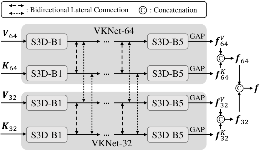
Figure 4: Our VKNet consists of two sub-networks, VKNet-64 and VKNet-32, which take video-keypoint pairs with different temporal receptive fields as inputs and output a set of vision features via global average pooling (GAP) layers. Within the VKNet, bidirectional lateral connections [9] are applied to the outputs of the first four S3D blocks (B1-B4) for video-video, keypoint-keypoint, and video-keypoint information exchange.

An illustration of the proposed video-keypoint network (VKNet) is shown in Figure 4. VKNet is composed of two sub-networks, namely VKNet-32 and VKNet-64, which take $(\boldsymbol{V}_{32},\boldsymbol{K}_{32})$ and $(\boldsymbol{V}_{64},\boldsymbol{K}_{64})$ as inputs, respectively. The network architectures of VKNet-32 and VKNet-64 are identical—either has a two-stream architecture consisting of a video encoder and a keypoint encoder. Since we denote keypoints as heatmaps, it is feasible to utilize any existing convolutional neural networks to extract keypoint features. In this work, S3D [57] with five blocks (B1–B5) is served as our video/keypoint encoder due to its excellent accuracy-speed trade-off. In our implementation, VKNet-32 (VKNet-64) is composed of two separate S3D networks with bidirectional lateral connections [9] applied to the outputs of the first four blocks (B1–B4). Specifically, VKNet-32 (VKNet-64) takes RGB video $\boldsymbol{V}_{32}$ ($\boldsymbol{V}_{64}$) and keypoint heatmap sequence $\boldsymbol{K}_{32}$ ($\boldsymbol{K}_{64}$) as inputs to extract the video feature $\boldsymbol{f}_{32}^{V}$ ($\boldsymbol{f}_{64}^{V}$) and the keypoint feature $\boldsymbol{f}_{32}^{K}$ ($\boldsymbol{f}_{64}^{K}$), respectively. We further concatenate $\boldsymbol{f}_{32}^{V}$ ($\boldsymbol{f}_{64}^{V}$) and $\boldsymbol{f}_{32}^{K}$ ($\boldsymbol{f}_{64}^{K}$) to generate $\boldsymbol{f}_{32}$ ($\boldsymbol{f}_{64}$) as the output of VKNet-32 (VKNet-64). The final feature $\boldsymbol{f}$ extracted by VKNet is the concatenation of $\boldsymbol{f}_{32}$ and $\boldsymbol{f}_{64}$.

It is worth mentioning that VKNet-32 and VKNet-64 are not two independent networks, we also introduce bidirectional lateral connections [9] to the corresponding encoders of the same input modality for video-video and keypoint-keypoint information exchange.

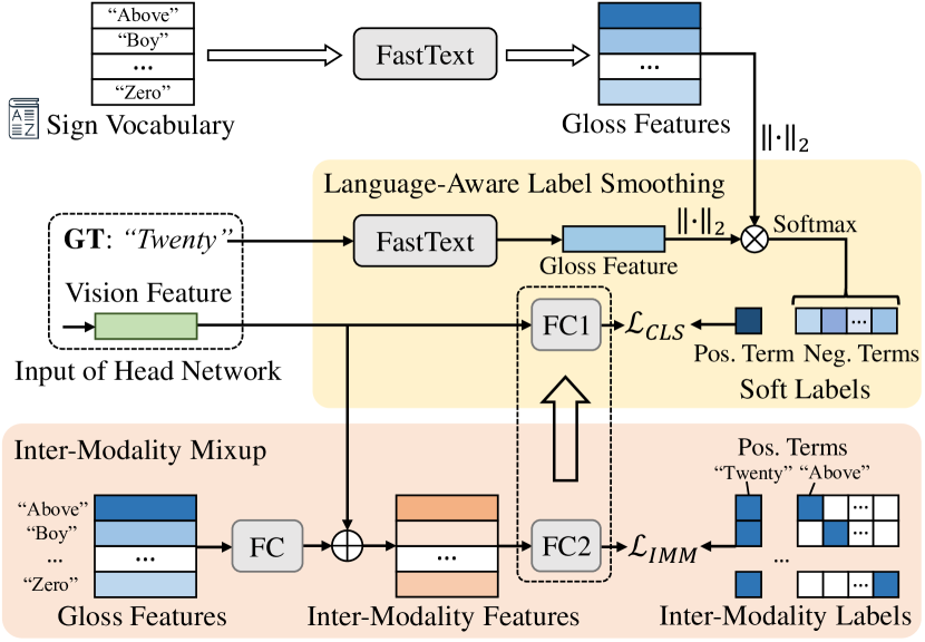
Figure 5: The architecture of our head network. Language-aware label smoothing generates soft labels whose smoothing weights are the normalized semantic similarities between the ground truth and remaining glosses within the sign vocabulary. Inter-modality mixup generates inter-modality features and the corresponding labels to maximize the signs’ separability in a latent space. Integration between FC1 and FC2 can further boost SLR performance.

3.3 Head Network

Figure 5 illustrates our head network, which is composed of a language-aware label smoothing branch and an inter-modality mixup branch.

3.3.1 Language-Aware Label Smoothing

The classical label smoothing [54, 14] was first proposed as a regularization technique to alleviate overfitting and make the model more adaptable. Specifically, given a training sample belonging to the $b$-th class, label smoothing replaces the one-hot label with a soft label $\boldsymbol{y}\in\mathbb{R}^{N}$ which is defined as:

$$\boldsymbol{y}[i]=\begin{cases}1-\epsilon\ &\text{if}\ i=b,\\ \epsilon/(N-1)\ &\text{otherwise},\end{cases}$$ (1)

where $\epsilon$ is a small constant (e.g., 0.2) and $N$ denotes the class number.

The vanilla label smoothing uniformly distributes $\epsilon$ to $N-1$ negative terms while the implicit semantics contained in glosses (sign labels) are ignored. In Section 1, we discuss the phenomenon that visually indistinguishable signs (VISigns) may have similar semantic meanings (finding-1). Motivated by this finding, we present a novel regularization strategy termed language-aware label smoothing, which assigns biased smoothing weights on the basis of semantic similarities of glosses to ease the training.

Gloss Features. Gloss is identified by a word which is associated with the sign’s semantic meaning. Thus any word representation learning framework can be adopted to extract gloss features for semantic similarity assessment. Concretely, given a sign vocabulary containing $N$ glosses, we leverage fastText [38] pretrained on Common Crawl to extract a 300-$d$ feature for each gloss. We use $\boldsymbol{E}\in\mathbb{R}^{N\times 300}$ to denote the $N$ gloss features.

Language-Aware Label Smoothing and Loss Function. As shown in Figure 5, given a training sample whose label is the $b$-th gloss, we first use fastText to extract its gloss feature $\boldsymbol{e}\in\mathbb{R}^{300}$. Then we compute the cosine similarities of the $b$-th gloss and all $N$ glosses within the sign vocabulary by $\boldsymbol{s}=\|\boldsymbol{E}\|_{2}\|\boldsymbol{e}\|_{2}^{T}\in\mathbb{R}^{N}$, where $\|\cdot\|_{2}$ denotes row-wise L2-norm. The proposed language-aware label smoothing generates a soft label $\boldsymbol{y}\in\mathbb{R}^{N}$ as:

$$\boldsymbol{y}[i]=\begin{cases}1-\epsilon\ &\text{if}\ i=b,\\ \epsilon\cdot\frac{\exp{(\boldsymbol{s}[i]/\tau)}}{\sum_{i=1,i\neq b}^{N}\exp{(\boldsymbol{s}[i]/\tau)}}\ &\text{otherwise},\end{cases}$$ (2)

where $\tau$ denotes a temperature parameter [5]. The classification loss $\mathcal{L}_{CLS}$ is a simple cross-entropy loss applied on the prediction and soft label $\boldsymbol{y}$.

3.3.2 Inter-Modality Mixup

In Section 1, we observe that VISigns may have distinct semantic meanings (finding-2), motivating us to make use of the semantic meanings of glosses to maximize signs’ separability in the latent space. To achieve the goal, as shown in Figure 5, we introduce the inter-modality mixup, which generates the inter-modality features by combining the vision feature and gloss features to predict the corresponding inter-modality labels.

Inter-Modality Mixup and Loss Function. Given the vision feature $\boldsymbol{f}\in\mathbb{R}^{D}$ extracted by our VKNet and the gloss features $\boldsymbol{E}\in\mathbb{R}^{N\times 300}$ encoded by the fastText, we first use a fully-connected (FC) layer to map $\boldsymbol{E}$ to the dimension of $N\times D$. After that, we integrate the vision feature $\boldsymbol{f}$ and the mapped gloss features $\bar{\boldsymbol{E}}$ via a broadcast addition operation into the inter-modality features $\boldsymbol{F}=\boldsymbol{f}+\bar{\boldsymbol{E}}\in\mathbb{R}^{N\times D}$. The $n$-th row of $\boldsymbol{F}$ (denoted as $\boldsymbol{F}^{n}$), which is the combination of the vision feature (whose corresponding ground truth is the $b$-th gloss) and the $n$-th gloss feature, is associated with the inter-modality labels $\boldsymbol{y}^{n}\in\mathbb{R}^{N}$:

$$\boldsymbol{y}^{n}[i]=\begin{cases}0.5\quad\text{if}\ i=b~{}\text{or}~{}i=n,\\ 0~{}~{}~{}\quad\text{otherwise}.\end{cases}$$ (3)

Note that as a special case, we set $\boldsymbol{y}^{n}[b]=1.0$ when $n=b$. Then we feed $\boldsymbol{F}^{n}$ into a classification layer to generate its prediction $\boldsymbol{p}^{n}\in(0,1)^{N}$, and use cross-entropy loss to approximate $\boldsymbol{y}^{n}$:

$$\mathcal{L}_{IMM}^{n}=-\sum_{i=1}^{N}\boldsymbol{y}^{n}[i]\text{log}(\boldsymbol{p}^{n}[i]).$$ (4)

Similarly, we could obtain the predictions of $N$ inter-modality features and their corresponding labels. The overall loss of inter-modality mixup is the average of $N$ cross-entropy losses:

$$\mathcal{L}_{IMM}=\frac{1}{N}\sum_{n=1}^{N}\mathcal{L}_{IMM}^{n}.$$ (5)

It is worth noting that $\mathcal{L}_{IMM}$ is an auxiliary loss and we drop the inter-modality mixup branch in the inference stage.

Boost Sign Language Recognition via the Integrated Classification Layer. As shown in Figure 5, we term the classification layer in the language-aware label smoothing branch and inter-modality mixup branch as FC1 and FC2, respectively. Though the inter-modality mixup only attends the training, the well-optimized FC2 contains implicit knowledge of recognizing signs with the help of language information. This inspires us to integrate FC2 into FC1 to boost sign language recognition. Concretely, the parameters of the FC1 are updated by a weighted sum of its own parameters and the FC2’s parameters at each iteration, which can be formulated as:

$$\begin{split}\theta_{1},\theta_{2}&\leftarrow\text{optimizer}(\theta_{1},\theta_{2},\nabla_{\theta_{1}}\mathcal{L},\nabla_{\theta_{2}}\mathcal{L},\eta)\\ \theta_{1}&\leftarrow\mu\theta_{1}+(1-\mu)\theta_{2},\end{split}$$ (6)

where $\theta_{1}$ and $\theta_{2}$ denote the parameters of FC1 and FC2, respectively, $\mathcal{L}$ is the overall loss of the head network introduced in Section 3.3.3, $\eta$ is the learning rate, and $\mu$ controls the contribution of $\theta_{2}$.

Method	MSASL1000				MSASL500				MSASL200				MSASL100
	Per-instance		Per-class		Per-instance		Per-class		Per-instance		Per-class		Per-instance		Per-class
	Top-1	Top-5	Top-1	Top-5	Top-1	Top-5	Top-1	Top-5	Top-1	Top-5	Top-1	Top-5	Top-1	Top-5	Top-1	Top-5
I3D [4]	–	–	57.69	81.08	–	–	72.50	89.80	–	–	81.97	93.79	–	–	81.76	95.16
I3D+BLSTM [4, 15]	40.99	–	–	–	–	–	–	–	–	–	–	–	72.07	–	–	–
ST-GCN [60]	36.03	59.92	32.32	57.15	–	–	–	–	52.91	76.67	54.20	77.62	59.84	82.03	60.79	82.96
BSL (multi-crop) [2]	64.71	85.59	61.55	84.43	–	–	–	–	–	–	–	–	–	–	–	–
TCK$\dagger$ [35]	–	–	–	–	–	–	–	–	80.31	91.82	81.14	92.24	83.04	93.46	83.91	93.52
HMA [18]	69.39	87.42	66.54	86.56	–	–	–	–	85.21	94.41	86.09	94.42	87.45	96.30	88.14	96.53
BEST [66]	71.21	88.85	68.24	87.98	–	–	–	–	86.83	95.66	87.45	95.72	89.56	96.96	90.08	97.07
SignBERT$\dagger$ [17]	71.24	89.12	67.96	88.40	–	–	–	–	86.98	96.39	87.62	96.43	89.56	97.36	89.96	97.51
NLA-SLR (Ours)	72.56	89.12	69.86	88.48	81.62	93.09	81.36	93.39	88.74	96.17	89.23	96.38	90.49	97.49	91.04	97.92
NLA-SLR (Ours, 3-crop)	73.80	89.65	70.95	89.07	82.90	93.46	83.06	93.54	89.48	96.69	89.86	96.93	91.02	97.89	91.24	98.19

Table 1: Comparison with previous works on MSASL. The results of I3D, I3D+BLSTM, and ST-GCN are reproduced by [25], [1], and [17], respectively. BSL achieves multi-crop inference by sliding a window with a stride of 8 frames. ($\dagger$denotes methods using extra data.)

3.3.3 Overall Loss

The loss $\mathcal{L}$ of the head network is the sum of the classification loss $\mathcal{L}_{CLS}$ and the inter-modality mixup loss $\mathcal{L}_{IMM}$ with a trade-off hyper-parameter $\gamma$: $\mathcal{L}=\mathcal{L}_{CLS}+\gamma\mathcal{L}_{IMM}$. Note that we apply the head network to each vision feature in Figure 4 independently, and the overall loss for the whole model is the sum of the loss of each head network.

3.4 Intra-Modality Mixup

We empirically find that Mixup [64] is helpful for sign language recognition. In contrast to the traditional Mixup which is applied to images and videos, we adopt the Mixup regularization on both RGB videos and keypoint heatmap sequences. For a distinction with our proposed Inter-Modality Mixup, we term the classical Mixup as Intra-Modality Mixup in our work.

4 Experiments

Method	WLASL2000				WLASL1000				WLASL300				WLASL100
	Per-instance		Per-class		Per-instance		Per-class		Per-instance		Per-class		Per-instance		Per-class
	Top-1	Top-5	Top-1	Top-5	Top-1	Top-5	Top-1	Top-5	Top-1	Top-5	Top-1	Top-5	Top-1	Top-5	Top-1	Top-5
OpenHands [51]	30.60	–	–	–	–	–	–	–	–	–	–	–	–	–	–	–
PSLR [55]	–	–	–	–	–	–	–	–	42.18	71.71	–	–	60.15	83.98	–	–
I3D [4]	32.48	57.31	–	–	47.33	76.44	–	–	56.14	79.94	–	–	65.89	84.11	–	–
ST-GCN [60]	34.40	66.57	32.53	65.45	–	–	–	–	44.46	73.05	45.29	73.16	50.78	79.07	51.62	79.47
Fusion-3 [16]	38.84	67.58	–	–	56.68	79.85	–	–	68.30	83.19	–	–	75.67	86.00	–	–
BSL (multi-crop) [2]	46.82	79.36	44.72	78.47	–	–	–	–	–	–	–	–	–	–	–	–
HMA [18]	51.39	86.34	48.75	85.74	–	–	–	–	–	–	–	–	–	–	–	–
TCK$\dagger$ [35]	–	–	–	–	–	–	–	–	68.56	89.52	68.75	89.41	77.52	91.08	77.55	91.42
BEST [66]	54.59	88.08	52.12	87.28	–	–	–	–	75.60	92.81	76.12	93.07	81.01	94.19	81.63	94.67
SignBERT$\dagger$ [17]	54.69	87.49	52.08	86.93	–	–	–	–	74.40	91.32	75.27	91.72	82.56	94.96	83.30	95.00
SAM-SLR* (5-crop) [23]	58.73	91.46	55.93	90.94	–	–	–	–	–	–	–	–	–	–	–	–
SAM-SLR-v2* (5-crop) [22]	59.39	91.48	56.63	90.89	–	–	–	–	–	–	–	–	–	–	–	–
NLA-SLR (Ours)	61.05	91.45	58.05	90.70	75.11	94.62	75.07	94.70	86.23	97.60	86.67	97.81	91.47	96.90	92.17	97.17
NLA-SLR (Ours, 3-crop)	61.26	91.77	58.31	90.91	75.64	94.62	75.72	94.65	86.98	97.60	87.33	97.81	92.64	96.90	93.08	97.17

Table 2: Comparison with previous works on WLASL. The results of I3D and ST-GCN are reproduced by [33] and [17], respectively. BSL achieves multi-crop inference by sliding a window with a stride of 8 frames. ($\dagger$denotes methods using extra data. *denotes methods using much more modalities than ours, e.g., optical flow, depth map, and depth flow.)

4.1 Datasets and Evaluation Metrics

Datasets. We evaluate our method on three public sign language recognition datasets: MSASL [25], WLASL [33], and NMFs-CSL [19]. MSASL is an American sign language (ASL) dataset with a vocabulary size of 1,000. It consists of 16,054, 5,287, and 4,172 samples in the training, development (dev), and test set, respectively. It also released three subsets consisting of only the top 500/200/100 most frequent glosses. WLASL is the latest ASL dataset with a larger vocabulary size of 2,000. It consists of 14,289, 3,916, and 2,878 samples in the training, dev, and test set, respectively. Similar to MSASL, it also released three subsets consisting of 1,000/300/100 frequent glosses. NMFs-CSL is a challenging Chinese sign language (CSL) dataset involving many fine-grained non-manual features (NMFs). It consists of 25,608 and 6,402 samples in the training and test set with a vocabulary size of 1,067. However, since the dataset owners only provide label indexes instead of glosses, we cannot apply inter-modality mixup on it, and we have to replace our language-aware label smoothing with the vanilla one.

Evaluation Metrics. Following [17, 18, 22], we report both per-instance and per-class accuracy, which denote the average accuracy over instances and classes, on the test sets. Note that since NMFs-CSL is a balanced dataset, i.e., each class contains equal amount of samples, we only report per-instance accuracy on it.

4.2 Implementation Details

Training Details and Hyper-parameters. The S3D backbone within VKNet-64/32 is first pretrained on Kinetics-400 [26]. Then we separately pretrain the video and keypoint encoder within VKNet-64/32 on SLR datasets. Finally, our VKNet is initialized with the pretrained VKNet-64 and VKNet-32. Data augmentations include spatial cropping with a range of [0.7-1.0] and temporal cropping. We adopt identical data augmentations for both RGB videos and heatmap sequences to maintain spatial and temporal consistency. Unless otherwise specified, we set $\lambda\sim Beta(0.8,0.8)$ for intra-modality mixup [64], and $\epsilon=0.2$ and $\tau=0.5$ in Eq. 2. Similar to [12], we gradually increase $\mu$ in Eq. 6 such that greater gradients of FC1 come from $\mathcal{L}_{CLS}$ in the late training stage since only FC1 is used during inference. Specifically, $\mu=1-(1-\mu_{base})\cdot(\cos{(\pi m/M)}+1)/2$, where $\mu_{base}=0.99$, $m$ is the current epoch, and $M$ is the maximum number of epochs. For the same reason, we gradually decrease the weight of $\mathcal{L}_{IMM}$ by $\gamma=(\cos{(\pi m/M)}+1)/2$. The whole model is trained with a batch size of 32 for 100 epochs. We use a cosine annealing schedule and an Adam optimizer [30] with a weight decay of $1e-3$ and an initial learning rate of $1e-3$.

Inference. We report results of single-crop and 3-crop inference for a comparison with state-of-the-art methods [2, 23, 22]. All ablation studies are conducted in the setting of single-crop inference. For 3-crop inference, we temporally crop videos at the start, middle, end of the raw video, and the average prediction is served as the final prediction. More details are in the supplementary materials.

4.3 Comparison with State-of-the-art Methods

Method	Top-1	Top-5
I3D◇ [4]	64.4	88.0
TSM◇ [36]	64.5	88.7
Slowfast◇ [11]	66.3	86.6
GLE-Net [19]	69.0	88.1
HMA [18]	75.6	95.3
SignBERT$\dagger$ [17]	78.4	97.3
BEST [66]	79.2	97.1
NLA-SLR (Ours)	83.4	98.3
NLA-SLR (Ours, 3-crop)	83.7	98.5

Table 3: Comparison with previous works on NMFs-CSL. (^◇methods reproduced by GLE-Net. $\dagger$methods using extra data.)

MSASL. Table 1 shows a comprehensive comparison between other methods and ours on all the sub-splits of MSASL. Our approach outperforms the previous best method SignBERT [17], which utilizes extra data, by 2.56%/2.50%/1.46% on the 1,000/200/100 sub-splits regarding the top-1 accuracy, respectively.

WLASL. We evaluate our method on all the sub-splits of WLASL as shown in Table 2. The previous state-of-the-art method, SAM-SLR-v2 [22], proposes a heavy multi-modal ensemble framework, which involves many modalities including RGB videos, keypoints, optical flow, depth map, and depth flow. However, our method significantly outperforms SAM-SLR-v2 by 1.87%/1.68% in terms of the per-instance/class top-1 accuracy while using much fewer modalities (only RGB videos and keypoints).

NMFs-CSL. Finally, as shown in Table 3, our approach also outperforms the previous best method BEST [66] by a large margin (83.7% vs. 79.2% on top-1 accuracy).

4.4 Ablation Studies

We conduct ablation studies on WLASL following [35, 22] due to its large vocabulary size.

VKNet. We first validate the effectiveness of our backbone, VKNet. As shown in Table 4, two-stream models, VKNet-32/64, can significantly outperform single-stream models, Video/Keypoint-32/64, which validates the effectiveness of modeling both videos and keypoints. Besides, 64-frame models can consistently outperform 32-frame ones as expected since longer inputs can provide more information for the model to classify sign videos. However, our VKNet performs better than a single 64-frame model, VKNet-64, especially on the top-5 accuracy, which implies that the 64-frame and 32-frame inputs can complement each other and the difference of the temporal receptive fields can bring more knowledge to model training.

Method	Per-instance		Per-class
	Top-1	Top-5	Top-1	Top-5
Video-32	45.73	81.10	42.69	79.90
Keypoint-32	46.66	79.95	43.81	78.49
VKNet-32	52.95	85.75	50.26	84.50
Video-64	51.15	83.43	48.14	82.20
Keypoint-64	49.10	82.00	46.18	80.71
VKNet-64	56.95	87.00	54.13	86.05
VKNet	57.19	88.29	54.35	87.49

Table 4: Ablation studies on VKNet.

Major Components of NLA-SLR. As shown in Table 5, we study the effects of the major components of our NLA-SLR framework: language-aware label smoothing (Lang-LS) and sign mixup (ensemble of the intra- and inter-modality mixup). First, Lang-LS can improve the performance of the baseline, VKNet, by 1.22%/1.11% on the top-1 and top-5 accuracy, respectively, which validates the effectiveness of language-aware soft labels. Besides, more performance gain comes from sign mixup, which significantly improves the top-1 accuracy from 57.19% to 60.32%. Finally, using both Lang-LS and sign mixup along with the VKNet can achieve the best performance: 61.05%/91.45% on the top-1 and top-5 accuracy, respectively. Note that both of the major components introduce negligible extra cost: Lang-LS simply replace the one-hot labels with the language-aware soft labels; sign mixup merely introduces two extra fully-connected layers (one for mapping gloss features and the other one for auxiliary training) for each head network, and both of them are dropped during inference.

VKNet	Lang-LS	Sign Mixup	Per-instance		Per-class
			Top-1	Top-5	Top-1	Top-5
✓			57.19	88.29	54.35	87.49
✓	✓		58.41	89.40	55.74	88.67
✓		✓	60.32	90.86	57.55	90.06
✓	✓	✓	61.05	91.45	58.05	90.70

Table 5: Ablation studies for the major components of NLA-SLR. (Lang-LS: language-aware label smoothing.)

Sign Mixup		Per-instance		Per-class
Intra-Modality	Inter-Modality	Top-1	Top-5	Top-1	Top-5
		58.41	89.40	55.74	88.67
✓		59.56	90.10	56.77	89.33
	✓	59.66	90.10	56.72	89.20
✓	✓	61.05	91.45	58.05	90.70

Table 6: Ablation studies on sign mixup which is composed of intra-modality and inter-modality mixup.

Sign Mixup. Our sign mixup is composed of two parts: intra-modality mixup, which extends the vanilla mixup [64] to keypoint heatmaps, and inter-modality mixup, which aims to maximize the signs’ separability with the help of language information. As shown in Table 6, either intra- or inter-modality mixup can improve the performance by more than 1% on the top-1 accuracy. In addition, intra- and inter-modality mixup are compatible—using both mixup techniques surpasses using either one of them.

Auxiliary	Inte-	Loss	Per-instance		Per-class
Classifier	gration	Weight Decay	Top-1	Top-5	Top-1	Top-5
			59.56	90.10	56.77	89.33
✓			59.87	90.31	57.07	89.57
✓	✓		60.84	91.07	57.99	90.28
✓	✓	✓	61.05	91.45	58.05	90.70

Table 7: Ablation studies for inter-modality mixup.

Inter-Modality Mixup. As shown in Table 7, we first study the effects of the auxiliary classifier, FC2 in Figure 5. It only slightly improves the performance (0.31% on top-1 accuracy). Most performance gain (almost 1% on the top-1 accuracy) comes from the integration of the two classifiers (FC1 and FC2 as described in Section 3.3.2). The reason is that it enables the natural language information to propagate from FC2 to FC1, which is the primary classifier during inference. Finally, the loss weight decay strategy of $\mathcal{L}_{IMM}$ also has a positive effect since it assures that more gradients for FC1 come from $\mathcal{L}_{CLS}$ in the late training stage.

Language-aware Label Smoothing. We conduct a comprehensive comparison between the vanilla label smoothing and our language-aware label smoothing (Lang-LS) by varying the smoothing parameter $\epsilon$ from 0.1 to 0.3. As shown in Table 8, our Lang-LS consistently outperforms the vanilla one regardless of the value of $\epsilon$. The results suggest that for SLR models, assigning biased smoothing weights to the soft labels on the basis of gloss feature similarities (Eq. 2) is a stronger regularization technique than the uniform distribution in the vanilla label smoothing (Eq. 1).

$\epsilon$	Type	Per-instance		Per-class
		Top-1	Top-5	Top-1	Top-5
0.1	Vanilla	59.83	90.72	56.90	90.10
	Language	60.15	91.35	57.30	90.68
0.2	Vanilla	60.11	91.00	57.09	90.34
	Language	61.05	91.45	58.05	90.70
0.3	Vanilla	60.01	90.97	57.01	90.12
	Language	60.49	91.31	57.44	90.67

Table 8: Comparison between the vanilla and language-aware label smoothing.

Method	VS-S	VS-D	Non-VS	Overall
VKNet	50.50	48.13	59.13	57.19
+Lang-LS	64.36	50.93	59.51	58.41
+Lang-LS, Inter-Mixup	65.35	56.07	60.07	59.66

Table 9: Quantitative results over VISigns. We report top-1 accuracy on WLASL2000. (VS-S/D: VISigns with similar/distinct semantic meanings.)

Presence and Quantitative Results of VISigns. To identify the VISigns appeared in the testing set, we first use our baseline model, VKNet, to get the highest prediction score $p_{1}$ (classified as gloss $g_{1}$) and the second highest prediction score $p_{2}$ (classified as gloss $g_{2}$) for each sample. Then we calculate the difference $\delta=p_{1}-p_{2}$. If $\delta\leq 0.1$, we regard $g_{1}$ and $g_{2}$ as potential VISigns. Next, we calculate the gloss similarity $s$ of $g_{1}$ and $g_{2}$ via FastText. If $s\geq 0.5$, we consider $g_{1}$ and $g_{2}$ as VS-S, otherwise, they are considered as VS-D. Finally, we invite native signers to filter out wrong cases. As a result, for WLASL with a vocabulary size of 2000, we get 101 instances covering 64 VS-S, 428 instances covering 270 VS-D, and 2349 instances covering 1666 non-VISigns (non-VS), respectively. As shown in Table 9, Lang-LS and Inter-Mixup yield the highest performance gains for VS-S (50.50 $\rightarrow$ 64.36) and VS-D (50.93 $\rightarrow$ 56.07), respectively, demonstrating that the improvements of our method derive from handling VISigns.

5 Conclusion

In this work, we propose Natural Language-Assisted Sign Language Recognition (NLA-SLR) framework, which leverages semantic information contained in glosses to promote sign language recognition. Specifically, we first propose language-aware label smoothing to ease model training by generating soft labels whose smoothing weights are the normalized semantic similarities. Second, to maximize the separability of signs with distinct semantic meanings, we propose inter-modality mixup which blends vision and gloss features as well as their labels. Besides, we also present a novel backbone, video-keypoint network, to model both RGB videos and human body keypoints and to absorb knowledge from sign videos of different temporal receptive fields. Empirically, our approach surpasses previous best methods on three widely-adopted benchmarks.

Acknowledgements. The work described in this paper was partially supported by a grant from the Research Grants Council of the HKSAR, China (Project No. HKUST16200118).

Appendix A More Implementation Details

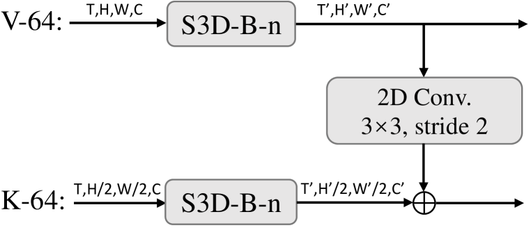
(a) Lateral connection from the 64-frame video encoder to the 64-frame keypoint encoder. We use a 2D convolution layer with a kernel size of $3\times 3$ and a stride of 2 to match the spatial resolutions. The same holds true for the 32-frame input.

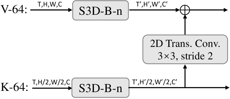
(b) Lateral connection from the 64-frame keypoint encoder to the 64-frame video encoder. We use a 2D transposed convolution layer with a kernel size of $3\times 3$ and a stride of 2 to match the spatial resolutions. The same holds true for the 32-frame input.

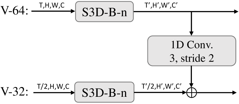
(c) Lateral connection from the 64-frame video encoder to the 32-frame one. We use a 1D convolution layer with a kernel size of 3 and a stride of 2 to match the temporal resolutions. The same holds true for the keypoint encoder.

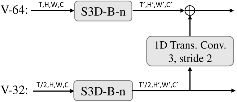
(d) Lateral connection from the 32-frame video encoder to the 64-frame one. We use a 1D transposed convolution layer with a kernel size of 3 and a stride of 2 to match the temporal resolutions. The same holds true for the keypoint encoder.

Figure 6: Illustration of the lateral connections. Note that we split bidirectional lateral connections into unidirectional ones for better illustration.

Bidirectional Lateral Connections. We apply bidirectional lateral connections [9] to the first four S3D blocks for video-video, keypoint-keypoint, and video-keypoint information exchange. For video-keypoint connections (dashed lines in Figure 4 in the main paper), since the input spatial resolutions of the video and keypoint encoder are $224\times 224$ and $112\times 112$, respectively, we use 2D convolution (Figure 6(a)) and transposed convolution layers (Figure 6(b)) with a stride of 2 and a kernel size of $3\times 3$ to match the spatial resolutions. For video-video and keypoint-keypoint connections (dotted dashed lines in Figure 4 in the main paper), due to the input length difference, we use 1D convolution (Figure 6(c)) and transposed convolution layers (Figure 6(d)) with a stride of 2 and a kernel size of 3 to match the temporal resolutions. Figure 6 shows the bidirectional lateral connections.

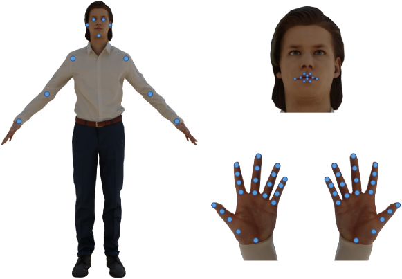
Figure 7: Illustration of the keypoints (11 upper body keypoints, 10 mouth keypoints, and 42 hand keypoints) used in our VKNet.

Keypoint Illustration. We show the keypoints used in our VKNet in Figure 7. The keypoints are estimated by HRNet [53] trained on COCO-WholeBody [24]. We use a subset of keypoints including 11 upper body keypoints, 10 mouth keypoints, and 42 hand keypoints.

Appendix B More Experiments

Head Choices for Inter-Modality Mixup. By default, we apply our inter-modality mixup on all head networks. To validate the effectiveness of this setting, we further conduct experiments on only applying it on partial heads. We categorize the head networks into three groups: video heads with input features $(\boldsymbol{f}_{64}^{V},\boldsymbol{f}_{32}^{V})$, keypoint heads with input features $(\boldsymbol{f}_{64}^{K},\boldsymbol{f}_{32}^{K})$, and joint heads with input features $(\boldsymbol{f}_{64},\boldsymbol{f}_{32},\boldsymbol{f})$. See Figure 4 in the main paper for their definitions. Table 10 shows that applying the inter-modality mixup on either one group of heads outperforms the baseline, and our default setting, applying the inter-modality mixup on all heads, achieves the best performance.

Video	Keypoint	Joint	Per-instance		Per-class
			Top-1	Top-5	Top-1	Top-5
			59.56	90.10	56.77	89.33
✓			60.42	91.07	57.62	90.37
	✓		60.08	90.62	57.27	89.76
		✓	59.83	90.72	56.88	90.11
✓	✓		60.56	91.24	57.87	90.37
✓	✓	✓	61.05	91.45	58.05	90.70

Table 10: Ablation studies on applying inter-modality mixup on different types of head networks.

Upper Body	Hand	Mouth	#Keypoints	Per-instance		Per-class
				Top-1	Top-5	Top-1	Top-5
✓			11	21.37	50.66	19.78	49.00
✓	✓		53	48.54	81.45	45.52	79.94
	✓	✓	52	48.64	81.83	45.64	80.36
✓	✓	✓	63	49.10	82.00	46.18	80.71

Table 11: Ablation study on keypoint selection.

Keypoint Selection. We utilize HRNet [53] trained on COCO-WholeBody [24] to estimate 63 keypoints (11 for upper body, 42 for hands, and 10 for mouth) per frame. As shown in Table 11, we validate the effectiveness of each keypoint group by training several single-stream keypoint encoders. Only using upper body keypoints yields the lowest top-1 accuracy (21.37%). Employing hand keypoints significantly improves the top-1 accuracy by 27.17%. This result is also consistent to the fact that sign languages mainly convey information by signers’ hand movement. Finally, the mouth keypoints also have a positive effect since signers usually mouth the words during signing.

V-V	K-K	V-K	Per-instance		Per-class
			Top-1	Top-5	Top-1	Top-5
			56.85	86.87	53.34	85.60
✓			57.12	87.11	54.21	85.94
✓	✓		57.16	87.56	54.03	86.54
✓	✓	✓	57.19	88.29	54.35	87.49

Table 12: Ablation studies on different types of bidirectional lateral connections. (V-V: video-video; K-K: keypoint-keypoint; V-K: video-keypoint.)

Bidirectional Lateral Connections. Within the VKNet, we apply bidirectional lateral connections [9] for video-video, keypoint-keypoint, and video-keypoint information exchange. See Figure 4 in the main paper for their illustration. As shown in Table 12, each type of bidirectional lateral connections has a positive effect on model performance, and our default setting, using all of the three types of the lateral connections, can achieve the best performance.

Method	Per-instance		Per-class
	Top-1	Top-5	Top-1	Top-5
SlowFast	56.81	87.60	53.69	86.68
VKNet	57.19	88.29	54.35	87.49

Table 13: Comparison between SlowFast and our VKNet.

VKNet vs. SlowFast. Our VKNet consists of two sub-networks, VKNet-64 and VKNet-32, to jointly model video-keypoint pairs with different temporal receptive fields. The results in Table 4 in the main paper suggest that modeling different video-keypoint pairs with varied temporal receptive fields improves the model generalization capability. One network that is related to our VKNet is SlowFast [11], which consists of two streams taking RGB videos with low/high frame rate as inputs while having a fixed temporal receptive field. For a fair comparison between SlowFast and our VKNet, we replace the “temporal crop” operation in Figure 3 in the main paper with “temporal sampling”, i.e., sampling a 32-frame pair from the 64-frame one with a stride of 2 frames, to mimic the SlowFast. As shown in Table 13, our VKNet can consistently outperform SlowFast on all of the four metrics, showing that VKNet is a stronger backbone for sign language recognition.

Method	Per-instance		Per-class
	Top-1	Top-5	Top-1	Top-5
Contrastive Learning	59.90	91.28	57.23	90.59
Inter-Modality Mixup	61.05	91.45	58.05	90.70

Table 14: Comparison between contrastive learning and our inter-modality mixup.

Inter-Modality Mixup vs. Contrastive Learning. Our inter-modality mixup blends vision and language features to better maximize the separability of signs. Its effectiveness is shown in Table 6 in the main paper. One work that is related to our inter-modality mixup is CLIP [45], which jointly trains an image encoder and a text encoder with a contrastive loss by maximizing the cosine similarity of positive image-text pairs while minimizing the similarity of negative pairs. Following the practice in CLIP, we replace our inter-modality mixup loss $\mathcal{L}_{IMM}$ with a contrastive loss between the vision feature $\boldsymbol{f}$ and gloss features $\bar{\boldsymbol{E}}$. As shown in Table 14, our inter-modality mixup can consistently outperform the contrastive learning method on all of the four metrics. The results demonstrate that our inter-modality mixup is a more effective approach to exploit semantic information contained in glosses.

Method	Per-instance		Per-class
	Top-1	Top-5	Top-1	Top-5
Word2vec [37]	60.63	91.14	57.53	90.42
GloVe [43]	60.81	90.90	57.73	90.27
FastText [38]	61.05	91.45	58.05	90.70
BERT [28]	60.11	90.83	57.15	90.05

Table 15: Comparison among different word representation learning methods.

Word Representation Learning Methods. We adopt fastText [38] as our default gloss feature extractor. Here we investigate other alternatives as shown in Table 15. Word2vec [37] and GloVe [43] are two classical word representation learning methods which are widely-adopted in NLP community. They perform comparably to each other that GloVe achieves better results on the top-1 accuracy while word2vec is superior regarding to the top-5 accuracy. As an improvement of word2vec, fastText leads to better results on all of the four metrics. Finally, we also utilize an advanced model, BERT-base [28], to extract word representations by averaging the outputs of the last layer. However, it performs worse than all the other methods since it is not dedicated to word representation learning.

Appendix C Visualization

Figure 8: Visualization of gloss feature similarities. We adopt fastText to extract gloss features.

Gloss Feature Similarity. The gloss feature similarities play a key role in our language-aware label smoothing. We select several glosses from the vocabulary and visualize the cosine similarities between their gloss features as a heatmap in Figure 8. We can see that the similarity matrix can roughly reflect the semantic similarities between glosses. For example, the pairs: (“adapt”, “change”), (“city”, “community”), (“cold”, “winter”), (“speech”, “oral”), and (“accent”, “voice”), have high similarities, which are consistent to human understanding.

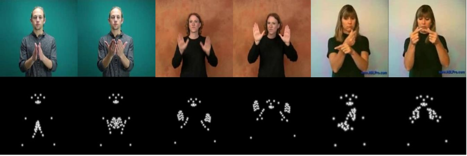
(a) WLASL2000.

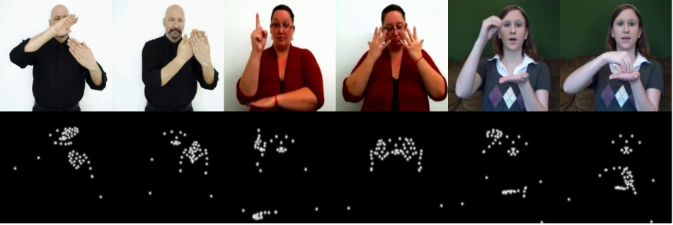
(b) MSASL1000.

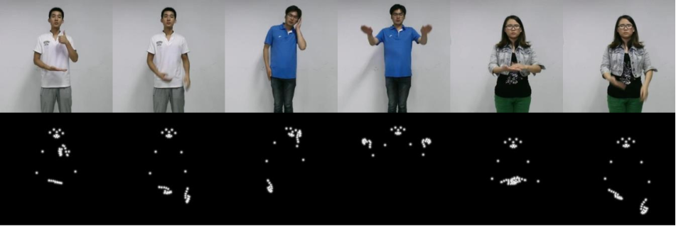
(c) NMFs-CSL.

Figure 9: Visualizations for the randomly selected frames and their corresponding keypoint heatmaps estimated by HRNet.

Keypoint Heatmaps. As shown in Figure 9, we visualize the keypoint heatmaps extracted by HRNet [53] by randomly selecting six frames of three signers from the test sets of WLASL2000, MSASL1000, and NMFs-CSL, respectively. We can clearly see that the heatmaps are robust to signer appearances, background variations, hand positions, and palm orientations.

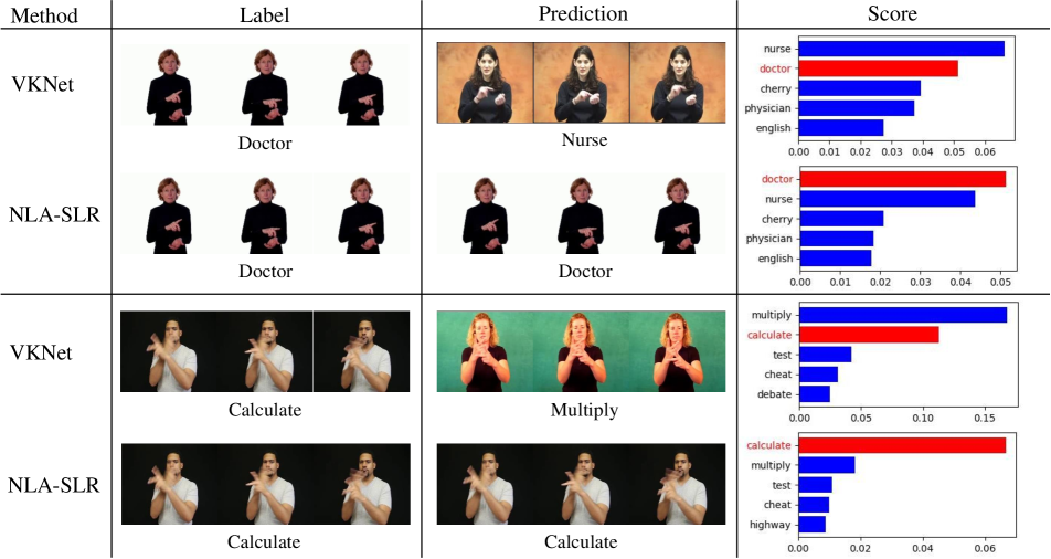
(a) VISigns with similar semantic meanings.

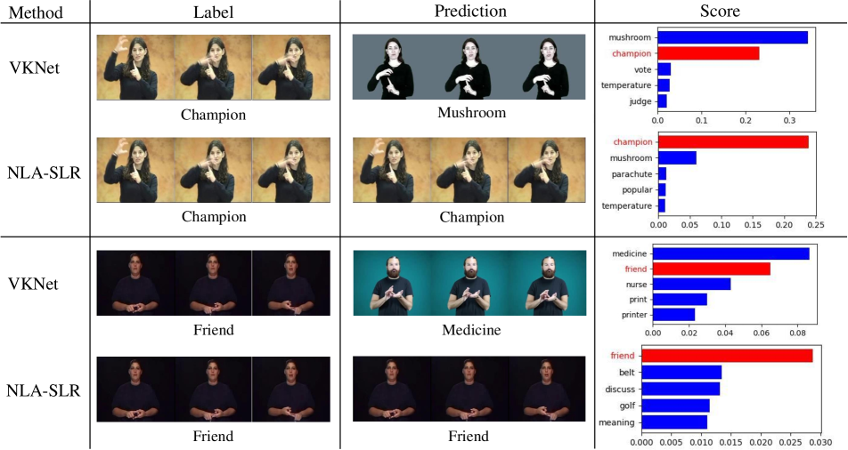
(b) VISigns with distinct semantic meanings.

Figure 10: Qualitative results on WLASL2000. (Here for NLA-SLR, we do not use intra-modality mixup for a fair comparison. The ground-truth gloss is highlighted in red.)

Appendix D Qualitative Results

As shown in Figure 10, we conduct qualitative analysis for our NLA-SLR. We find that compared with VKNet (baseline), our NLA-SLR can well classify visually indistinguishable signs (VISigns) with either similar or distinct meanings. As shown in Figure 10(a), our NLA-SLR can successfully distinguish (“doctor”, “nurse”) and (“calculate”, “multiply”), which are VISigns with similar semantic meanings, whereas the baseline, VKNet, fails to classify them. Besides, as shown in Figure 10(b), our NLA-SLR can also recognize VISigns with distinct semantic meanings: (“champion”, “mushroom”) and (“friend”, “medicine”). We owe these success to the two proposed techniques: language-aware label smoothing and inter-modality mixup.

Appendix E Social Impact and Limitation

Sign language is the primary communication method among the deaf community. Thus, research on sign language recognition can help bridge the communication gap between the normal-hearing and hearing-impaired people.

The proposed method is data-driven. Thus, the model performance may be affected by the biases in the training data. Besides, our backbone relies on pre-extracted keypoints; inaccurate keypoint estimation may hurt the model performance. We believe that stronger keypoint estimators may further improve sign language recognition in the future.

References

- [1] Nikolas Adaloglou, Theocharis Chatzis, Ilias Papastratis, Andreas Stergioulas, Georgios Th Papadopoulos, Vassia Zacharopoulou, George J Xydopoulos, Klimnis Atzakas, Dimitris Papazachariou, and Petros Daras. A comprehensive study on deep learning-based methods for sign language recognition. IEEE TMM, 24:1750–1762, 2021.
- [2] Samuel Albanie, Gül Varol, Liliane Momeni, Triantafyllos Afouras, Joon Son Chung, Neil Fox, and Andrew Zisserman. Bsl-1k: Scaling up co-articulated sign language recognition using mouthing cues. In ECCV, pages 35–53, 2020.
- [3] Piotr Bojanowski, Edouard Grave, Armand Joulin, and Tomas Mikolov. Enriching word vectors with subword information. Transactions of the association for computational linguistics, 5:135–146, 2017.
- [4] Joao Carreira and Andrew Zisserman. Quo vadis, action recognition? a new model and the kinetics dataset. In CVPR, 2017.
- [5] Ting Chen, Simon Kornblith, Mohammad Norouzi, and Geoffrey Hinton. A simple framework for contrastive learning of visual representations. In ICML, pages 1597–1607, 2020.
- [6] Yutong Chen, Fangyun Wei, Xiao Sun, Zhirong Wu, and Stephen Lin. A simple multi-modality transfer learning baseline for sign language translation. In CVPR, pages 5120–5130, 2022.
- [7] Yutong Chen, Ronglai Zuo, Fangyun Wei, Yu Wu, Shujie Liu, and Brian Mak. Two-stream network for sign language recognition and translation. In NeurIPS, 2022.
- [8] Yu Du, Fangyun Wei, Zihe Zhang, Miaojing Shi, Yue Gao, and Guoqi Li. Learning to prompt for open-vocabulary object detection with vision-language model. In CVPR, pages 14084–14093, 2022.
- [9] Haodong Duan, Yue Zhao, Kai Chen, Dahua Lin, and Bo Dai. Revisiting skeleton-based action recognition. In CVPR, pages 2969–2978, 2022.
- [10] Amanda Duarte, Samuel Albanie, Xavier Giró-i Nieto, and Gül Varol. Sign language video retrieval with free-form textual queries. In CVPR, pages 14094–14104, 2022.
- [11] Christoph Feichtenhofer, Haoqi Fan, Jitendra Malik, and Kaiming He. Slowfast networks for video recognition. In ICCV, pages 6202–6211, 2019.
- [12] Jean-Bastien Grill, Florian Strub, Florent Altché, Corentin Tallec, Pierre Richemond, Elena Buchatskaya, Carl Doersch, Bernardo Avila Pires, Zhaohan Guo, Mohammad Gheshlaghi Azar, et al. Bootstrap your own latent-a new approach to self-supervised learning. NeurIPS, 33:21271–21284, 2020.
- [13] Jiaxi Gu, Xiaojun Meng, Guansong Lu, Lu Hou, Minzhe Niu, Xiaodan Liang, Lewei Yao, Runhui Huang, Wei Zhang, Xin Jiang, et al. Wukong: A 100 million large-scale chinese cross-modal pre-training benchmark. In Thirty-sixth Conference on Neural Information Processing Systems Datasets and Benchmarks Track, 2022.
- [14] Tong He, Zhi Zhang, Hang Zhang, Zhongyue Zhang, Junyuan Xie, and Mu Li. Bag of tricks for image classification with convolutional neural networks. In CVPR, pages 558–567, 2019.
- [15] Sepp Hochreiter and Jürgen Schmidhuber. Long short-term memory. Neural Computation, 9(8):1735–1780, 1997.
- [16] Al Amin Hosain, Panneer Selvam Santhalingam, Parth Pathak, Huzefa Rangwala, and Jana Kosecka. Hand pose guided 3D pooling for word-level sign language recognition. In WACV, pages 3429–3439, 2021.
- [17] Hezhen Hu, Weichao Zhao, Wengang Zhou, Yuechen Wang, and Houqiang Li. Signbert: Pre-training of hand-model-aware representation for sign language recognition. In ICCV, pages 11087–11096, 2021.
- [18] Hezhen Hu, Wengang Zhou, and Houqiang Li. Hand-model-aware sign language recognition. In AAAI, volume 35, pages 1558–1566, 2021.
- [19] Hezhen Hu, Wengang Zhou, Junfu Pu, and Houqiang Li. Global-local enhancement network for nmf-aware sign language recognition. ACM transactions on multimedia computing, communications, and applications (TOMM), 17(3):1–19, 2021.
- [20] Tony Huang, Jack Chu, and Fangyun Wei. Unsupervised prompt learning for vision-language models. arXiv preprint arXiv:2204.03649, 2022.
- [21] Chao Jia, Yinfei Yang, Ye Xia, Yi-Ting Chen, Zarana Parekh, Hieu Pham, Quoc Le, Yun-Hsuan Sung, Zhen Li, and Tom Duerig. Scaling up visual and vision-language representation learning with noisy text supervision. In ICML, pages 4904–4916, 2021.
- [22] Songyao Jiang, Bin Sun, Lichen Wang, Yue Bai, Kunpeng Li, and Yun Fu. Sign language recognition via skeleton-aware multi-model ensemble. arXiv preprint arXiv:2110.06161, 2021.
- [23] Songyao Jiang, Bin Sun, Lichen Wang, Yue Bai, Kunpeng Li, and Yun Fu. Skeleton aware multi-modal sign language recognition. In CVPRW, pages 3413–3423, 2021.
- [24] Sheng Jin, Lumin Xu, Jin Xu, Can Wang, Wentao Liu, Chen Qian, Wanli Ouyang, and Ping Luo. Whole-body human pose estimation in the wild. In ECCV, pages 196–214, 2020.
- [25] Hamid Reza Vaezi Joze and Oscar Koller. Ms-asl: A large-scale data set and benchmark for understanding American sign language. In BMVC, 2019.
- [26] Will Kay, Joao Carreira, Karen Simonyan, Brian Zhang, Chloe Hillier, Sudheendra Vijayanarasimhan, Fabio Viola, Tim Green, Trevor Back, Paul Natsev, et al. The kinetics human action video dataset. arXiv preprint arXiv:1705.06950, 2017.
- [27] Bo Ke, Yunquan Zhu, Mengtian Li, Xiujun Shu, Ruizhi Qiao, and Bo Ren. Hyperspherical learning in multi-label classification. In ECCV, pages 38–55, 2022.
- [28] Jacob Devlin Ming-Wei Chang Kenton and Lee Kristina Toutanova. BERT: Pre-training of deep bidirectional transformers for language understanding. In NAACL-HLT, pages 4171–4186, 2019.
- [29] Youngwook Kim, Jae Myung Kim, Zeynep Akata, and Jungwoo Lee. Large loss matters in weakly supervised multi-label classification. In CVPR, pages 14156–14165, 2022.
- [30] Diederik P. Kingma and Jimmy Ba. Adam: A method for stochastic optimization. In ICLR, 2015.
- [31] Gihyun Kwon and Jong Chul Ye. Clipstyler: Image style transfer with a single text condition. In CVPR, pages 18062–18071, 2022.
- [32] Boyi Li, Kilian Q Weinberger, Serge Belongie, Vladlen Koltun, and Rene Ranftl. Language-driven semantic segmentation. In ICLR, 2021.
- [33] Dongxu Li, Cristian Rodriguez, Xin Yu, and Hongdong Li. Word-level deep sign language recognition from video: A new large-scale dataset and methods comparison. In WACV, pages 1459–1469, 2020.
- [34] Dongxu Li, Chenchen Xu, Xin Yu, Kaihao Zhang, Ben Swift, Hanna Suominen, and Hongdong Li. Tspnet: Hierarchical feature learning via temporal semantic pyramid for sign language translation. In NeurIPS, 2020.
- [35] Dongxu Li, Xin Yu, Chenchen Xu, Lars Petersson, and Hongdong Li. Transferring cross-domain knowledge for video sign language recognition. In CVPR, pages 6205–6214, 2020.
- [36] Ji Lin, Chuang Gan, and Song Han. Tsm: Temporal shift module for efficient video understanding. In ICCV, pages 7083–7093, 2019.
- [37] Tomas Mikolov, Kai Chen, Greg Corrado, and Jeffrey Dean. Efficient estimation of word representations in vector space. arXiv preprint arXiv:1301.3781, 2013.
- [38] Tomas Mikolov, Edouard Grave, Piotr Bojanowski, Christian Puhrsch, and Armand Joulin. Advances in pre-training distributed word representations. In Proceedings of the International Conference on Language Resources and Evaluation (LREC), 2018.
- [39] Yuecong Min, Aiming Hao, Xiujuan Chai, and Xilin Chen. Visual alignment constraint for continuous sign language recognition. In ICCV, pages 11542–11551, October 2021.
- [40] Andriy Mnih and Koray Kavukcuoglu. Learning word embeddings efficiently with noise-contrastive estimation. NeurIPS, 26, 2013.
- [41] Liliane Momeni, Hannah Bull, KR Prajwal, Samuel Albanie, Gül Varol, and Andrew Zisserman. Automatic dense annotation of large-vocabulary sign language videos. In ECCV, pages 671–690, 2022.
- [42] Or Patashnik, Zongze Wu, Eli Shechtman, Daniel Cohen-Or, and Dani Lischinski. Styleclip: Text-driven manipulation of stylegan imagery. In ICCV, pages 2085–2094, 2021.
- [43] Jeffrey Pennington, Richard Socher, and Christopher D Manning. Glove: Global vectors for word representation. In EMNLP, pages 1532–1543, 2014.
- [44] Zhaofan Qiu, Ting Yao, and Tao Mei. Learning spatio-temporal representation with pseudo-3D residual networks. In ICCV, pages 5533–5541, 2017.
- [45] Alec Radford, Jong Wook Kim, Chris Hallacy, Aditya Ramesh, Gabriel Goh, Sandhini Agarwal, Girish Sastry, Amanda Askell, Pamela Mishkin, Jack Clark, et al. Learning transferable visual models from natural language supervision. In ICML, pages 8748–8763, 2021.
- [46] Sai Rajeswar, Pau Rodriguez, Soumye Singhal, David Vazquez, and Aaron Courville. Multi-label iterated learning for image classification with label ambiguity. In CVPR, pages 4783–4793, 2022.
- [47] Yongming Rao, Wenliang Zhao, Guangyi Chen, Yansong Tang, Zheng Zhu, Guan Huang, Jie Zhou, and Jiwen Lu. Denseclip: Language-guided dense prediction with context-aware prompting. In CVPR, pages 18082–18091, 2022.
- [48] Tal Ridnik, Emanuel Ben-Baruch, Nadav Zamir, Asaf Noy, Itamar Friedman, Matan Protter, and Lihi Zelnik-Manor. Asymmetric loss for multi-label classification. In ICCV, pages 82–91, 2021.
- [49] Olga Russakovsky, Jia Deng, Hao Su, Jonathan Krause, Sanjeev Satheesh, Sean Ma, Zhiheng Huang, Andrej Karpathy, Aditya Khosla, Michael S. Bernstein, Alexander C. Berg, and Fei-Fei Li. Imagenet large scale visual recognition challenge. IJCV, 2014.
- [50] Wendy Sandler and Diane Lillo-Martin. Sign language and linguistic universals. Cambridge University Press, 2006.
- [51] Prem Selvaraj, Gokul Nc, Pratyush Kumar, and Mitesh M Khapra. Openhands: Making sign language recognition accessible with pose-based pretrained models across languages. In ACL, pages 2114–2133, 2022.
- [52] Bowen Shi, Diane Brentari, Greg Shakhnarovich, and Karen Livescu. Open-domain sign language translation learned from online video. arXiv preprint arXiv:2205.12870, 2022.
- [53] Ke Sun, Bin Xiao, Dong Liu, and Jingdong Wang. Deep high-resolution representation learning for human pose estimation. In CVPR, pages 5693–5703, 2019.
- [54] Christian Szegedy, Vincent Vanhoucke, Sergey Ioffe, Jon Shlens, and Zbigniew Wojna. Rethinking the inception architecture for computer vision. In CVPR, pages 2818–2826, 2016.
- [55] Anirudh Tunga, Sai Vidyaranya Nuthalapati, and Juan Wachs. Pose-based sign language recognition using gcn and bert. In WACVW, pages 31–40, 2021.
- [56] Gül Varol, Liliane Momeni, Samuel Albanie, Triantafyllos Afouras, and Andrew Zisserman. Scaling up sign spotting through sign language dictionaries. IJCV, 130(6):1416–1439, 2022.
- [57] Saining Xie, Chen Sun, Jonathan Huang, Zhuowen Tu, and Kevin Murphy. Rethinking spatiotemporal feature learning: Speed-accuracy trade-offs in video classification. In ECCV, pages 305–321, 2018.
- [58] Jiarui Xu, Shalini De Mello, Sifei Liu, Wonmin Byeon, Thomas Breuel, Jan Kautz, and Xiaolong Wang. Groupvit: Semantic segmentation emerges from text supervision. In CVPR, pages 18134–18144, 2022.
- [59] Mengde Xu, Zheng Zhang, Fangyun Wei, Yutong Lin, Yue Cao, Han Hu, and Xiang Bai. A simple baseline for zero-shot semantic segmentation with pre-trained vision-language model. arXiv preprint arXiv:2112.14757, 2021.
- [60] Sijie Yan, Yuanjun Xiong, and Dahua Lin. Spatial temporal graph convolutional networks for skeleton-based action recognition. In AAAI, 2018.
- [61] Lewei Yao, Runhui Huang, Lu Hou, Guansong Lu, Minzhe Niu, Hang Xu, Xiaodan Liang, Zhenguo Li, Xin Jiang, and Chunjing Xu. FILIP: Fine-grained interactive language-image pre-training. In ICLR, 2022.
- [62] Aoxiong Yin, Zhou Zhao, Weike Jin, Meng Zhang, Xingshan Zeng, and Xiaofei He. MLSLT: Towards multilingual sign language translation. In CVPR, pages 5109–5119, 2022.
- [63] Aoxiong Yin, Zhou Zhao, Jinglin Liu, Weike Jin, Meng Zhang, Xingshan Zeng, and Xiaofei He. Simulslt: End-to-end simultaneous sign language translation. In MM, pages 4118–4127, 2021.
- [64] Hongyi Zhang, Moustapha Cisse, Yann N Dauphin, and David Lopez-Paz. mixup: Beyond empirical risk minimization. In ICLR, 2018.
- [65] Min-Ling Zhang and Zhi-Hua Zhou. A review on multi-label learning algorithms. IEEE TKDE, 26(8):1819–1837, 2013.
- [66] Weichao Zhao, Hezhen Hu, Wengang Zhou, Jiaxin Shi, and Houqiang Li. BEST: BERT pre-training for sign language recognition with coupling tokenization. In AAAI, 2023.
- [67] Hao Zhou, Wengang Zhou, Yun Zhou, and Houqiang Li. Spatial-temporal multi-cue network for continuous sign language recognition. In AAAI, pages 13009–13016, 2020.
- [68] Kaiyang Zhou, Jingkang Yang, Chen Change Loy, and Ziwei Liu. Learning to prompt for vision-language models. IJCV, 130(9):2337–2348, 2022.
- [69] Ronglai Zuo and Brian Mak. C2SLR: Consistency-enhanced continuous sign language recognition. In CVPR, pages 5131–5140, 2022.
- [70] Ronglai Zuo and Brian Mak. Local context-aware self-attention for continuous sign language recognition. In Proc. Interspeech, pages 4810–4814, 2022.