Machine Learning the Tip of the Red Giant Branch

Abstract

A novel method for investigating the sensitivity of the tip of the red giant branch (TRGB) I band magnitude $M_{I}$ to stellar input physics is presented. We compute a grid of $\sim$125,000 theoretical stellar models with varying mass, initial helium abundance, and initial metallicity, and train a machine learning emulator to predict $M_{I}$ as a function of these parameters. First, our emulator can be used to theoretically predict $M_{I}$ in a given galaxy using Monte Carlo sampling. As an example, we predict $M_{I}=-3.84^{+0.14}_{-0.12}$ in the Large Magellanic Cloud. Second, our emulator enables a direct comparison of theoretical predictions for $M_{I}$ with empirical calibrations to constrain stellar modeling parameters using Bayesian Markov Chain Monte Carlo methods. We demonstrate this by using empirical TRGB calibrations to obtain new independent measurements of the metallicity in three galaxies. We find $Z=0.0117^{+0.0083}_{-0.0055}$ in the Large Magellanic Cloud, $Z=0.0077^{+0.0074}_{-0.0038}$ in NGC 4258, and $Z=0.0111^{+0.0083}_{-00.0056}$ in $\omega$-Centauri, consistent with other measurements. Other potential applications of our methodology are discussed.

1 Introduction

The tip of the red giant branch (TRGB) is an important tool in modern astronomy. Its consistency in the I band (Johnsons-Cousins) across different environments (Sakai 1999, Freedman et al. 2019, Riess et al. 2021b) enables its use as a standardizable candle. Empirically, the TRGB feature in the colour-magnitude diagram can be calibrated with errors of order $10\%$ (Yuan et al. 2019, Freedman et al. 2019, 2020, Riess et al. 2021b, Anand et al. 2022). Theoretical predictions from stellar modeling codes are far less precise due to uncertainties affecting the physics of the helium flash coming from environmental factors such as metallicity and the input physics required for stellar modeling e.g., opacity, mixing length, nuclear reaction rates, and large errors in the bolometric corrections needed to compute the I band magnitude, $M_{I}$ (Serenelli et al. 2017, Saltas & Tognelli 2022).

In the context of the Hubble tension (Abdalla et al. 2022), different calibrations of the TRGB $M_{I}$ in the Large Magellanic Cloud (LMC) result in a distance ladder measurement of the Hubble constant, $H_{0}$, that is either in tension with the value inferred using the cosmic microwave background (CMB) (Yuan et al. 2019, Soltis et al. 2021, Riess et al. 2021a, Anand et al. 2022, Anderson et al. 2023), or is consistent with it (Freedman et al. 2019, 2020). A better theoretical understanding of the TRGB and its associated uncertainties may aid in validating competing empirical calibrations.

One major factor limiting theoretical studies is the run-time needed to simulate stars at the TRGB, which is typically of the order of two hours or more. In this work, we present a novel method to overcome this whereby a large grid ($\sim\!\!125,000$ models) with varying mass, initial helium abundance, and initial metallicity is simulated and used to train a machine learning (ML) emulator. This emulator evaluates in milliseconds, enabling rapid sampling of parameter space. We showcase two applications of our emulator. First, we estimate the theoretical error on the TRGB $M_{I}$ by performing a Monte Carlo (MC) sampling of the parameter space. We predict $M_{I}=-3.84^{+0.14}_{-0.12}$ in the LMC. Second, we use empirical calibrations of $M_{I}$ in the LMC, $\omega$-Centauri, and NGC 4258 to constrain these objects’ metallicity, $Z$, by using Markov Chain Monte Carlo (MCMC) sampling. Our results are summarized in Table 1. In the case of the LMC, we find results consistent with previous studies that use different methods. The other two objects studied do not have reported metallicity measurements.

A reproduction package accompanies this work and can be found at the following URL: https://zenodo.org/record/7197580. This includes our entire grid of models, MESA inlists needed to reproduce them, our ML emulators, and our MC and MCMC python scripts used to produce the results presented here.

This paper is organized as follows. In section 2 we describe the grid of models used to train the ML emulator. In section 3 we describe the ML methods we use to train our emulator. In section 4.1 we use MC sampling to predict the theoretical TRGB $M_{I}$ in the LMC. In section 4.2 we use MCMC sampling to constrain the metallicity in the LMC, NGC 4258, and $\omega$-Centauri. We discuss our results in section 5 and conclude in section 6.

2 Theoretical TRGB Models

2.1 Stellar modeling

We ran a grid of 124,844 models with varying mass, $M$, initial helium abundance, $Y$, and initial metallicity, $Z$, from the pre-main-sequence to the onset of the helium flash (defined as the time when the power in helium burning exceeds $10^{6}$ ergs/s) using the stellar structure code – Modules for Experiments in Stellar Astrophysics MESA version 12778 (Paxton et al. 2011, Paxton et al. 2013, 2015, 2018, 2019, Jermyn et al. 2022). The parameters were varied over the ranges $0.7{\rm M}_{\odot}\leq M\leq 2.25{\rm M}_{\odot}$, $0.2\leq Y\leq 0.3$, and $10^{-5}\leq Z\leq 0.04$. The spacing is uniform across our parameters. This spacing is sufficient for efficient machine learning with the small number of parameters we varied but we note that higher dimensional parameter spaces would require more efficient sampling methods e.g., Latin hypercube sampling. The parameter ranges were chosen to cover the entire parameter space that is expected to experience a core helium flash (Hansen et al. 2004, Kippenhahn et al. 2013). In the case of $Y$, we chose a range that does not differ significantly from the primordial helium mass fraction but is broad enough to include possible enhancements from previous generations of stars. Other stellar modeling parameters corresponding to the choice of input physics were fixed to fiducial values. In particular, the mixing length $\alpha_{MLT}=1.8$, the nuclear reaction rates were set to the MESA defaults (a combination of NACRE and REACLIB (Angulo et al. 1999, Cyburt et al. 2010)), mass loss on the red giant branch (RGB) follows the Reimer’s prescription (Reimers 1975) with efficiency parameter $\eta=0.1$, and we used the initial elemental abundances reported by Grevesse & Sauval (1998) (GS98). MESA inlists containing all of our parameter choices can be found in our reproduction package Dennis & Sakstein (2022). Fixing the input physics was necessary for two reasons. First, the accuracy of the ML emulator will likely decrease as additional parameters are varied, and it is important that the errors in our analysis are not driven by the errors in the ML. For this reason, we chose to investigate the effects of parameters where stochastic variation between stars due to mass and environment are expected. (Said another way, even if other parameters such as mixing length and wind loss efficiency are known perfectly, there will still be variations in $M_{I}$ due to $M$, $Y$ and $Z$ between different stars.) Ultimately, we found that the emulator was highly accurate (see section 3); so it is likely that more parameters can be varied without degrading the accuracy. Our preliminary work is then a proof of concept. Second, a large number of grid points is necessary to achieve an accurate ML emulator, and each additional parameter must have proportionate representation. Our grid with three parameters varying consumed one million CPU hours. Fixing the other parameters enabled the grid generation to be computationally tractable. We discuss the possibility of varying additional parameters in section 5.

2.2 Bolometric and Color Corrections

The theoretical I band magnitude $M_{I}$ for each grid model and its empirical error $\Delta M_{I}$, which are what is needed for our MCMC comparison with empirical $M_{I}$ calibrations, were calculated using the Worthey & Lee (Worthey & Lee 2011) bolometric correction code. Our reproduction package (Dennis & Sakstein 2022) includes a machine learning emulator (not used in this work, see section 3) that instead predicts the luminosity $L$, the effective temperature $T_{\rm eff}$, the surface gravity $\log(g)$, and the iron abundance $[{\rm Fe}/{\rm H}]$. These can be used to calculate $M_{I}$ and $\Delta M_{I}$ using alternative bolometric corrections e.g., MARCS (Gustafsson et al. 2008), or PHOENIX (Dotter et al. 2008). We comment that users interested in using other bolometric corrections could apply them directly to our data set and train a new ML emulator using our codes provided. This will likely produce more accurate results than applying the bolometric corrections to our ML predictions for the MESA outputs.

The range of $M$, $Y$, and $Z$ covered by our grid covers the entire parameter space where a core helium flash is expected (Hansen et al. 2004, Kippenhahn et al. 2013), however, since the boundary between these objects and other objects is not uniform across parameter space, some of our models do not contribute to the TRGB. In particular, some models (low $M$ and $Z$ boundaries) do not reach the TRGB in a time shorter than the age of the universe. Others burn helium stably in their core before the TRGB (high $M$ and high $Z$ boundaries). They do not experience a core flash but do experience shell flashes. Excluding these models from the grid would bias the ML emulator to predict a core flash for parameters that do not give rise to one (within the age of the universe), so we instead train an additional ML emulator that classifies models as either older than the age of the universe, core helium burning, or core helium flashing (see section 3). The former two are assigned zero likelihood in our MCMC analysis (see section 4.2) and are excluded from our MC analysis. We manually exclude these models from the training set for the emulator that predicts $M_{I}$ and $\Delta M_{I}$. A small number of models failed to converge. These were removed from the grid since they are too few in number to effect the ML.

In addition to bolometric corrections, a galaxy-dependent color correction must be applied to $M_{I}$. The I band magnitude is a function of $(V-I)$, with each reported empirical calibration being the zero-point with respect to some reference $(V-I)$. In order to enable a like-for-like comparison, our ML predicted $M_{I}$ must be converted to a prediction at the reference $(V-I)$. We accomplish this using the empirical color corrections listed in Table 1.

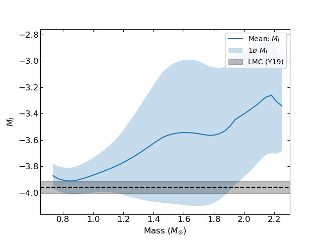
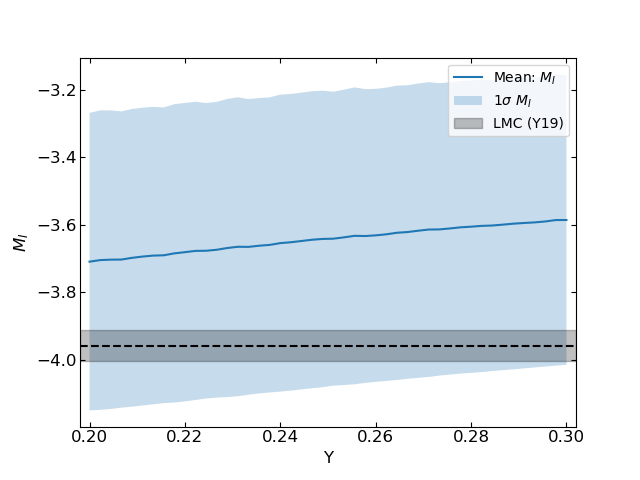
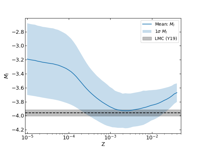
Figure 1: Variation in the TRGB $M_{I}$ with varying parameters indicated in the subfigures. The mean $M_{I}$ in each bin was found by averaging over the other parameters. The error bands show the 1$\sigma$ deviation from the mean in each bin. The gray horizontal band shows the Yuan et al. (2019) empirical $M_{I}$ calibration with $1\sigma$ errors.

2.3 Grid of Models

The results of our grids (with models that reach the TRGB in a time longer than the age of the universe and models that experience stable core helium burning removed) are exemplified in Figure 1. The figures show the average value of $M_{I}$ and the standard deviation in bins of varying $M$, $Y$, and $Z$ after applying the color correction appropriate for the empirical calibration of Yuan et al. (2019). Other color corrections yield similar results. The figures illustrate the effects of degeneracies across parameter space. A band showing the calibration of $M_{I}$ from is included in dark gray for reference Yuan et al. (2019). There is a weak correlation between initial helium abundance and $M_{I}$, but the other two parameters show interesting features. Larger initial masses exhibit a dimmer $M_{I}$ on average and show a larger spread in the possible values. More stars are rejected as too old or shell flashing at the low edge of mass and the high edge of metallicity, resulting in narrower standard deviations across the respective bins. At higher masses, the majority of the additional mass becomes part of the stellar envelope, reducing the opacity, which dims the resulting flash. Turning to metallicity, there is a peak in brightness around $10^{-3}$. At very low metallicities, the opacity is lower but there are fewer metals for the CNO cycle, which yields a higher brightness than pp-chain burning. The luminosity at the TRGB (which is set by the hydrogen burning shell at the onset of the helium flash) is therefore dimmer than at higher $Z$. The reduced brightness at very high metallicities is due to the increased opacity that results from the the increased number of electrons, which reduces photon the mean free path. The balance between these two extremes determines the peak brightness.

3 Machine Learning Emulator

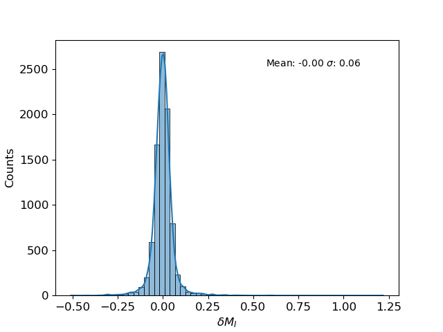
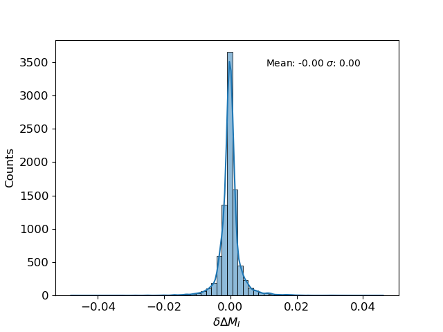
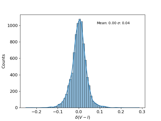
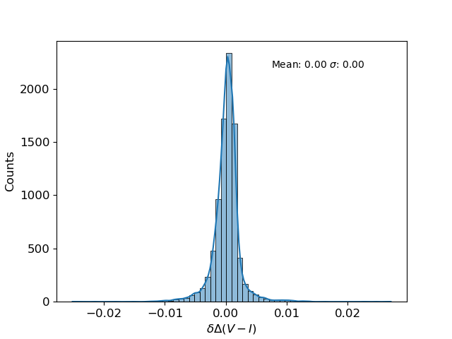
Figure 2: Error distributions for $M_{I}$, $\Delta M_{I}$, $(V-I)$, and $\Delta(V-I)$ from the ML regression. These distributions were found by subtracting the ML predictions from the true values found by applying the bolometric correction code to each grid point that reached the TRGB in a time shorter than the age of the universe.

We trained a ML emulator on the grid of models described in the previous section. We used a deep neural network (DNN) with the tensorflow (Abadi et al. 2015) and keras packages (Chollet et al. 2015) to build the emulator because of advantage DNNs hold over other ML methods in high dimensional parameter spaces. We implemented the network using the ADAM (Kingma & Ba 2014) optimizer and hand tuned the hyperparameters of the network to optimize the training results. We remark that other methods, e.g., explored in Liashchynskyi & Liashchynskyi (2019) may be necessary for higher dimensional data sets. The ML emulator was built in two components, a classifier that evaluates whether or not a set of input parameters $\{M,Y,Z\}$ will yield a star on the TRGB (or whether they will exhibit stable core helium burning, or reach TRGB in a time longer than the age of the universe), and a regression algorithm that predicts $M_{I}$; the empirical error in the I band, $\Delta M_{I}$; the $(V-I)$ colour; and the empirical error in the $(V-I)$ colour, $\Delta(V-I)$, for given $\{M,Y,Z\}$. We also trained, a separate ML regression algorithm that takes $\{M,Y,Z\}$ as inputs, but instead outputs the raw MESA outputs, luminosity $L$, effective temperature $T_{\rm eff}$, surface gravity $\log(g)$, and iron abundance $[{\rm Fe}/{\rm H}]$. This emulator had a longer evaluation time and was less accurate than the emulator above so was not used in this work. We provide this as part of our reproduction package Dennis & Sakstein (2022) for readers interested in using different bolometric corrections.

Both algorithms used an 80%/10%/10% split between training, validation, and testing data, but the training data set for the classifier was re-sampled using SMOTE (Chawla et al. 2011) due to the large imbalance between the three classes which can have a negative affect on the network (Sui et al. 2019). SMOTE creates synthetic data by taking convex combinations of groups of data points in the minority class, randomly sampling within the convex combinations until the all the classes have an equal number of data points. This yields a balanced data set which is better for the ML training because an unbalanced dataset can bias the network towards labeling more objects as the more populous class. The classification algorithm has an accuracy of 99.7% and a categorical crossentropy loss of 0.01 across the three categories. The regression algorithm used predicts $M_{I}$, $\Delta M_{I}$, $(V-I)$, and $\Delta(V-I)$ with a mean squared error loss of $3.24\times 10^{-5}$ for input data and corresponding output values normalized between 0 and 1. Histograms of the residuals from the testing data set for $M_{I}$, $\Delta M_{I}$, $(V-I)$, and $\Delta(V-I)$ are shown in Figure 2. The errors in our ML algorithm are highly subdominant to those coming from the empirical bolometric corrections, which have an average error of order $0.1$ mag.

4 Results

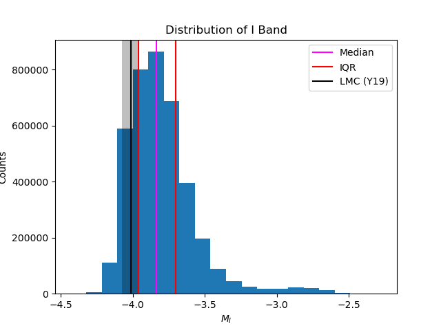
Figure 3: The distribution of $M_{I}$ after Monte Carlo sampling was performed on the parameter space $\{M,Y,Z\}$ and passed through the ML network (including error accounting) applying the colour correction from corresponding to the LMC. The gray band shows the zero point $M_{I}$ in the LMC reported by Yuan et al. (2019) (with 1$\sigma$ errors) and the magenta lines (IQR) indicate the interquartile range. The prior distributions were taken to be uniform on all parameters (left panel) and uniform on $M$ and $Y$ with a Gaussian prior on the metallicity $Z=0.0097\pm 0.0007$ (right panel).

4.1 Theoretical I Band Calibration

In this section we estimate the theoretical error in $M_{I}$ due to variations in $M$, $Y$, and $Z$ by performing Monte Carlo sampling. We performed 5,000,000 random draws assuming each parameter is uniformly distributed across our parameter range i.e., no prior knowledge of the input parameters was assumed except for the ML classifier which excludes models that do not contribute the TRGB. We note that this analysis assumes that the TRGB $M_{I}$ is due solely to a single star. We discuss caveats to this assumption in section 5. For each draw, the empirical error in the bolometric correction was accounted for by drawing from a Gaussian distribution with zero mean and standard deviation $\Delta M_{I}$ predicted by our emulator for each point and adding it to the predicted $M_{I}$. The errors in the ML predictions were accounted for by drawing from the distributions shown in Figure 2 and adding the result to the corresponding ML prediction. The error in the ML is highly subdominant to the empirical bolometric correction errors. Additionally, a colour correction was applied to the ML prediction. For this example, we used the correction found by Yuan et al. (2019) in the LMC given in Table 1. The resulting distribution is shown in the left panel of Figure 3. We predict $M_{I}=-3.84^{+0.14}_{-0.12}$ (median and interquartile range) in the LMC. This prediction is consistent with the value of $M_{I}$ reported by Yuan et al. (2019).

Tighter predictions can be made by placing stronger priors on the parameters. For example, suppose that one was interested in modeling some galaxy or globular cluster for which an independent measurement of the metallicity is available. One could then place a Gaussian prior on the metallicity to obtain a narrower distribution for $M_{I}$. As an example, Keller & Wood (2006) report $Z=0.0097\pm 0.0007$ in the LMC by fitting non-linear Cepheid pulsation models. Imposing this prior, we predict the median and interquartile range of $M_{I}$ to be $M_{I}=-3.92^{+0.09}_{-0.08}$ in the LMC. The resulting distribution is shown in the right panel of Figure 3. We caution that imposing strong priors such as these may come with caveats that imply larger errors. For example, a recent analysis of LMC Cepheids using a Bayesian MCMC method that accounts for degeneracies due to nuisance parameters in non-linear pulsation models (Desmond et al. 2021) found far larger error bars on the metallicity ($\mathcal{O}(0.01)$).

4.2 Comparison of Theoretical and empirically-calibrated I Band Magnitudes

In this section we demonstrate how using ML to emulate the theoretical TRGB $M_{I}$ can enable comparisons of theory and observation that account for degeneracies by using MCMC sampling to constrain the metallicity in the LMC, NGC 4258, and $\omega$-Centauri, all of which have reported empirical calibrations of $M_{I}$. We use the empirical calibrations reported by Jang & Lee (2017) for NCG 4258, Bellazzini et al. (2001) for $\omega$-Centauri, and Jang & Lee (2017) for the LMC but with a zero point adjustment to the value reported by Yuan et al. (2019).

The MCMC analysis was performed using the emcee package (Foreman-Mackey et al. 2013) assuming uniform priors on $M$, $Y$, and $Z$ with ranges $0.7{\rm M}_{\odot}\leq M\leq 2.25{\rm M}_{\odot}$, $0.2\leq Y\leq 0.3$, and $10^{-5}\leq Z\leq 10^{-2}$. The ML classification algorithm was used within the MCMC to assign zero-likelihood to models whose input parameters would give rise to models that burn helium stably in the core or models that are older than the age of the universe. The log-likelihood function was taken to be Gaussian i.e.,

$$\ln{\mathcal{L}}=-\frac{1}{2}\left[\left(\frac{M_{I,\textrm{obs}}-f(\textrm{ML}(\theta)_{I},\textrm{ML}(\theta)_{(V-I)})^{2}}{\sigma_{\textrm{tot}}}\right)^{2}\right.~{}\\ +\left.~{}\ln(2\pi\sigma_{\textrm{tot}}^{2})\vphantom{\sum^{N}_{i=1}}\right],$$ (1)

where $M_{I,\textrm{obs}}$ is the observed I Band calibration, ML$(\theta)_{I}$ and ML$(\theta)_{(V-I)}$ are the predictions for $M_{I}$ and $(V-I)$ from the ML emulator for a given set of parameters $\theta$, and $f(M_{I},(V-I))$ is the empirical calibration given in Table 1 for each galaxy. $\sigma_{\textrm{tot}}$ is given by

$$\sigma_{\textrm{tot}}^{2}=\sigma_{\textrm{obs}}^{2}+\sigma_{f}^{2},$$ (2)

where $\sigma_{\textrm{obs}}$ is the error on the empirical I band calibration and the error $\sigma_{f}$ in the calibration $f$ is given by

$$\sigma_{f}\approx\left|\frac{\partial f}{\partial M_{I}}\right|^{2}\Delta{M_{I}}^{2}+\left|\frac{\partial f}{\partial(V-I)}\right|^{2}\Delta{(V-I)}^{2}+\\ 2\left|\frac{\partial f}{\partial M_{I}}\right|\left|\frac{\partial f}{\partial(V-I)}\right|\Delta{M_{I}}\Delta{(V-I)}\rho_{M_{I}(V-I)},$$ (3)

where $M_{I}$ and $(V-I)$ are the ML predictions for the I band magnitude and $(V-I)$, $\Delta M_{I}$ and $\Delta{(V-I)}$ are their associated empirical errors from the bolometric corrections, and $\rho_{M_{I}(V-I)}$ is the correlation between $M_{I}$ and $(V-I)$ which was calculated by taking the covariance of the two variables from the full simulation dataset.

The error on the machine learning in $M_{I}$, $\Delta M_{I}$, $(V-I)$, and $\Delta(V-I)$ was included by randomly drawing values from the distributions given in Figure 2 and adding them to the values predicted by the ML emulator for each set of parameters $\theta$ sampled. This is similar to the procedure used by McClintock et al. (2019). These errors are highly subdominant to the errors on the calibration and the bolometric correction. We determined convergence by demanding that the autocorrelation time $\tau$ was less than 0.1% the length of the chain and that it had changed by less than 1% over the previous 10,000 steps (Goodman & Weare 2010, Sokal 1997). In all cases we found that the MCMC converged within 120,000 steps, but we allowed it to continue to 500,000 to ensure that the walker was no longer influenced by its starting location. We discarded half of the sampler as burn-in.

A corner plot showing the results of the MCMC for the LMC is given in Figure 4. The corner plots for the other systems we studied are visually similar and are included in the appendix in Figures 5, and 6.

Figure 4: Posterior distributions of each parameter for the $M_{I}$ calibration in the LMC. Both 2D and marginalized posteriors are shown. The values for the medians and interquartile range are given in 1. The contours represent the 68%, 95%, and 99% confidence intervals. 

Evidently, the mass and initial helium abundance are poorly constrained. The underlying reason for this can be seen in Figure 1 where one can see that the empirical calibration can be reproduced by masses and initial helium abundances that span the majority of the range that give rise to a core helium flash. Conversely, we find a constraint on the metallicity $0.0077^{+0.0074}_{-0.0038}$. This is consistent with other measurements that give $Z\sim 0.008$ (e.g., Schaerer et al. (1993), Keller & Wood (2006), Kołaczkowski & Pigulski (2006), Glatt et al. (2010), Marconi et al. (2013), Choudhury et al. (2021)). As evidenced by Figure 1, there is only a narrow range of $Z$ that can reproduce the calibration, hence the constraint. Our analyses of NGC 4258 and $\omega$-Centauri yielded similar results, which are given in Table 1. Our bounds can be understood as a volume effect by considering Figure 1 where one can see that the preferred region of parameter space corresponds to the range of $Z$ with the largest number of models (per unit $Z$) can match the calibration.

There is little difference between the measurements we report in Table 1 despite significant differences in the calibrations. The cause of this are the large errors in the bolometric corrections that are necessary to compute $M_{I}$ from the output of stellar structure codes. These are of the order $\Delta M_{I}\sim 0.1$. The next largest source of error are the calibrations themselves. Imposing strong priors could improve these bounds, provided that the independent measurement informing that prior is reliable.

Target	Reference	$M_{I}$	Colour Correction	Mass (${\rm M}_{\odot}$)	$Z$
LMC	Yuan et al. (2019)	$-3.958\pm 0.046$	$0.091[(V-I)-1.5]^{2}-0.007[(V-I)-1.5]$	$1.590^{+0.222}_{-0.287}$	$0.0117^{+0.0083}_{-0.0055}$
NGC 4258	Jang & Lee (2017)	$-4.016\pm 0.058$	$0.091[(V-I)-1.5]^{2}-0.007[(V-I)-1.5]$	$1.530^{+0.218}_{-0.270}$	$0.0077^{+0.0074}_{-0.0038}$
$\omega$ Centauri	Bellazzini et al. (2001)	$-4.012\pm 0.12$	$-0.046(V-I)+0.08(V-I)^{2}$	$1.56^{+0.221}_{-0.277}$	$0.0111^{+0.0083}_{-00.0056}$

Table 1: Empirical $M_{I}$ calibrations, associated error, colour corrections, and the parameter constraints found by the MCMC for each target galaxy. The median and interquartile range are reported for $M$ and $Z$. The $Y$ parameter is not included as the posterior is essentially flat and uninformative. We choose to report the median and interquartile ranges rather than the mean and standard deviation due to the highly non-Gaussian nature of the marginalized posteriors. Note that the LMC calibration is identical to NGC 4258 but with a shifted zero point.

5 Discussion

In this section we discuss the limitations of our methodology presented above, and suggest improvements to our preliminary exploration that could ameliorate these in future studies. We also discuss potential applications of our emulator to other areas of cosmology and astronomy.

5.1 Limitations of Our Methodology

The first limitation of our study is is that we have fixed the input physics e.g., the opacity, mixing length, nuclear reaction rates etc. Our analysis therefore includes stochastic variations due to environment and mass but not uncertainties in the input physics. Fixing the input physics made our procedure computationally tractable and we were able to run 124,844 models in one million CPU hours (using eight cores per model). As an example, varying five parameters instead of three would require a one million model grid to train the machine learning emulator with acceptable errors. This would require approximately 16 million CPU hours assuming 16 steps in each parameter. A second reason we fixed the input physics was to test the efficiency of the ML emulator, which generally degrades with more free parameters. Our results indicate that all input physics parameters could be varied without significantly degrading the ML accuracy, however, we remark that more efficient sampling e.g., Latin hypercube sampling or active learning (Rocha et al. 2022) may reduce the number of models needed to obtain the same accuracy. Varying a larger number of parameters would be computationally feasible if a larger number of CPUs were available to us. We also remark that the it is possible to take derivatives of DNNs, which enables the use of Hamiltonian MCMC which is more efficient than standard MCMC in higher dimensions.

A second limitation is that we assumed the TRGB $M_{I}$ is due solely to a single star. In practice, there are many stars near the TRGB and an edge detection method (e.g. Lee et al. (1993)) is used to determine the calibration. Future work could allow for a more direct comparison by using our ML emulators to stochastically generate mock color-magnitude diagrams and apply the same edge-fitting methods to generate theoretical predictions. One could then estimate the theoretical error by repeating this process several times.

A final limitation is that our analysis includes statistical errors but not systematic errors. We have used a single stellar structure code (MESA) and assumed that its predictions are accurate. Any potential missing physics is not accounted for. For example, MESA is a one-dimensional code and is missing the physics of three-dimensional processes. Furthermore, we have made discrete choices for input physics such as boundary conditions, elemental abundances, and numerical solver. Different choices may result in systematically different $M_{I}$ predictions. Finally, we used the WL bolometric corrections but there are alternatives such as MARCS (Gustafsson et al. 2008) or PHOENIX (Dotter et al. 2008) that may give systematically different results. It would be interesting to repeat this work using different stellar structure codes, different choice for input physics, and/or different bolometric corrections and compare the results.

5.2 Applications to Cosmology and Astronomy

5.2.1 Validating Competing Empirical $M_{I}$ Calibrations

The empirical calibration of $M_{I}$ in the LMC is currently the subject of intense discussion in the context of the Hubble tension (Verde et al. 2019, Abdalla et al. 2022). The LMC calibration we adopted for this study (Yuan et al. 2019) gives a value of Hubble’s constant, $H_{0}$, that is consistent with the Cepheid-calibrated distance ladder Riess et al. (2021a) but in $\sim$5$\sigma$ tension with the value inferred from the CMB. An alternative calibration was reported by Freedman et al. (2020) that is consistent with the CMB. It would be interesting to explore whether these differing calibrations effect our results but, unfortunately, the color correction reported by Freedman et al. (2020) is only valid over a narrow range of $(V-I)$ (spanning $(V-I)=1.8\pm 0.4$), and our models extend to values outside of this range so we are unable to perform such a comparison.

If a color correction that is valid over our entire range of $(V-I)$ were available then it may be possible to validate one of these comparisons by demanding consistency of metallicity measurement with independent measurements of the metallicity (e.g., Schaerer et al. (1993), Keller & Wood (2006), Kołaczkowski & Pigulski (2006), Glatt et al. (2010), Marconi et al. (2013), Choudhury et al. (2021)). It is possible that the large errors due to the bolometric corrections discussed above may result in overlapping $Z$ measurements for both LMC calibrations, in which case this validation method would first require the errors on the empirical bolometric corrections to be reduced.

5.2.2 Constraining Stellar modeling Parameters

Our preliminary analysis has revealed that it is possible to vary more parameters without a significant degradation of the machine learning emulator’s accuracy. Varying stellar modeling parameters that control the input physics such as the mixing length, radiative opacity, and nuclear reaction rates — which are all highly uncertain — and emulating the results would enable measurements of these parameters to be made using the MCMC methods we have developed here.

The constraining power of our method can be improved by simultaneously fitting multiple calibrations in either the same or different galaxies. There are two contributions to the theoretical error on $M_{I}$: a stochastic component due to environment-dependent quantities such as mass, metallicity, helium abundance, and mass-loss; and uncertainties in the input physics. Each empirical calibration should be consistent with a universal set of input physics parameters. Simultaneously fitting multiple calibrations allowing $M$, $Y$, $Z$, and mass-loss to vary between systems while demanding that the input physics parameters are universal across all systems will then improve the bounds. As an example, Górski et al. (2018) report $M_{I}$ for 19 systems in the Small and Large Magellanic Clouds. They also report magnitudes in the J, K, and H bands that could provide even more constraining power.

6 Summary and Conclusion

In this work we have presented a novel methodology to explore the effects of environment and input physics on the TRGB $M_{I}$. We simulated a grid of 124,844 stellar models with varying mass, initial helium abundance, and metallicity and used this to train a machine learning emulator to predict $M_{I}$ as a function of these parameters. We used this to perform a Monte Carlo analysis where we randomly drew 500,000 sets of parameters (assuming them to be independently uniformly distributed) to derive a theoretical distribution for $M_{I}$. We predict $M_{I}=-3.84^{+0.14}_{-0.12}$ in the LMC. It is likely the true uncertainty is larger since we fixed the input physics. This paper is accompanied by a reproduction package that contains our emulator, and the grid of models used to train it (Dennis & Sakstein 2022).

Our emulator enables a direct comparison of theoretical and empirical I band calibrations using Markov Chain Monte Carlo analyses. These require run-times of order seconds or shorter to be computationally efficient so performing an individual stellar structure simulation (which takes two or more hours depending on the number of available cores) for each parameter draw is not feasible. Our emulator evaluates in milliseconds and can therefore overcome this barrier. As an example, we used calibrations in the LMC, NGC 4258, and $\omega$-Centauri to constrain the metallicity of these systems. Our results are summarized in Table 1.

Our results are subject to several limitations discussed in section 5. If these can be overcome then our methodology could be used to measure stellar modeling parameters, or for validating competing empirical $M_{I}$ calibrations to the LMC that are the source of much discussion in the context of the Hubble tension.

We conclude by noting that the techniques we have introduced here are applicable to other areas of stellar astronomy. Possible applications include emulating stellar pulsation codes to constrain Cepheid and RR Lyrae properties using MCMC (particularly for such objects in detached eclipsing binaries (Desmond et al. 2021)), and emulating main-sequence models for use in isochrone fitting.

7 Acknowledgements

We thank Adrian Ayala, Aaron Dotter, Robert Farmer, Frank Timmes, and the wider MESA community for answering our MESA-related questions. We are grateful for conversations with Eric J. Baxter, Djuna Croon, Samuel D. McDermott, Harry Desmond, Noah Franz, Marco Gatti, Dan Hey, Esther Hu, Jason Kumar, Danny Marfatia, Marco Raveri, Ippocratis Saltas, Xerxes Tata, Brent Tully, Guy Worthey, Dan Huber, and Jen van Saders. We are especially thankful to David Rubin for providing detailed comments and answering our many questions, and to David Schanzenbach for his assistance with using the University of Hawai​​​​ ‘ ​​​​i supercomputer MANA.

Our simulations were run on the University of Hawai‘i’s high-performance supercomputer MANA. The technical support and advanced computing resources from University of Hawai‘i Information Technology Services – Cyberinfrastructure, funded in part by the National Science Foundation MRI award #1920304, are gratefully acknowledged.

Data Availability

All data used in this work are publicly available in our reproduction package Dennis & Sakstein (2022).

Software

MESA version 12778, MESASDK version 20200325, Worthey and Lee Bolometric Correction Code Worthey & Lee (2011), NumPy version 1.22.3 (Harris et al. 2020), Pandas version 1.4.3 (Wes McKinney 2010, pandas development team 2020), Matplotlib version 3.5.1 (Hunter 2007), Tensorflow version 2.4.1 (Abadi et al. 2015, Chollet et al. 2015), corner version 2.2.1 (Foreman-Mackey 2016), emcee version 3.1.2 (Foreman-Mackey et al. 2013).

appendix

In this section we show the corner plots for our MCMC analyses of the TRGB $M_{I}$ empirical calibrations in $\omega$-Centauri, and NGC 4258. See section 4.2 for more details.

Figure 5: Same as Figure 1 but for the $M_{I}$ calibration in $\omega$-Centauri. 

Figure 6: Same as Figure 1 but for the $M_{I}$ calibration in NGC 4258.

References

- Abadi et al. (2015) Abadi M., et al., 2015, TensorFlow: Large-Scale Machine Learning on Heterogeneous Systems, https://www.tensorflow.org/
- Abdalla et al. (2022) Abdalla E., et al., 2022, JHEAp, 34, 49
- Anand et al. (2022) Anand G. S., Tully R. B., Rizzi L., Riess A. G., Yuan W., 2022, ApJ, 932, 15
- Anderson et al. (2023) Anderson R. I., Koblischke N. W., Eyer L., 2023, arXiv e-prints, p. arXiv:2303.04790
- Angulo et al. (1999) Angulo C., et al., 1999, Nucl. Phys. A, 656, 3
- Bellazzini et al. (2001) Bellazzini M., Ferraro F. R., Pancino E., 2001, ApJ, 556, 635
- Chawla et al. (2011) Chawla N. V., Bowyer K. W., Hall L. O., Kegelmeyer W. P., 2011, Journal of Artificial Intelligence Research, p. arXiv:1106.1813
- Chollet et al. (2015) Chollet F., et al., 2015, Keras, https://keras.io
- Choudhury et al. (2021) Choudhury S., et al., 2021, MNRAS, 507, 4752
- Cyburt et al. (2010) Cyburt R. H., et al., 2010, ApJS, 189, 240
- Dennis & Sakstein (2022) Dennis M. T., Sakstein J., 2022, Machine Learning the Tip of the Red Giant Branch, doi:10.5281/zenodo.7197580, https://doi.org/10.5281/zenodo.7197580
- Desmond et al. (2021) Desmond H., Sakstein J., Jain B., 2021, Phys. Rev. D, 103, 024028
- Dotter et al. (2008) Dotter A., Chaboyer B., Jevremović D., Kostov V., Baron E., Ferguson J. W., 2008, ApJS, 178, 89
- Foreman-Mackey (2016) Foreman-Mackey D., 2016, The Journal of Open Source Software, 1, 24
- Foreman-Mackey et al. (2013) Foreman-Mackey D., Hogg D. W., Lang D., Goodman J., 2013, PASP, 125, 306
- Freedman et al. (2019) Freedman W. L., et al., 2019, ApJ, 882, 34
- Freedman et al. (2020) Freedman W. L., et al., 2020, ApJ, 891, 57
- Glatt et al. (2010) Glatt K., Grebel E. K., Koch A., 2010, A&A, 517, A50
- Goodman & Weare (2010) Goodman J., Weare J., 2010, Communications in Applied Mathematics and Computational Science, 5, 65
- Górski et al. (2018) Górski M., et al., 2018, AJ, 156, 278
- Grevesse & Sauval (1998) Grevesse N., Sauval A. J., 1998, Space Sci. Rev., 85, 161
- Gustafsson et al. (2008) Gustafsson B., Edvardsson B., Eriksson K., Jørgensen U. G., Nordlund Å., Plez B., 2008, A&A, 486, 951
- Hansen et al. (2004) Hansen C. J., Kawaler S. D., Trimble V., 2004, Stellar interiors : physical principles, structure, and evolution
- Harris et al. (2020) Harris C. R., et al., 2020, Nature, 585, 357
- Hunter (2007) Hunter J. D., 2007, Computing in Science and Engineering, 9, 90
- Jang & Lee (2017) Jang I. S., Lee M. G., 2017, ApJ, 835, 28
- Jermyn et al. (2022) Jermyn A. S., et al., 2022, arXiv e-prints, p. arXiv:2208.03651
- Keller & Wood (2006) Keller S. C., Wood P. R., 2006, ApJ, 642, 834
- Kingma & Ba (2014) Kingma D. P., Ba J., 2014, arXiv e-prints, p. arXiv:1412.6980
- Kippenhahn et al. (2013) Kippenhahn R., Weigert A., Weiss A., 2013, Stellar Structure and Evolution, doi:10.1007/978-3-642-30304-3.
- Kołaczkowski & Pigulski (2006) Kołaczkowski Z., Pigulski A., 2006, in Randich S., Pasquini L., eds, Chemical Abundances and Mixing in Stars in the Milky Way and its Satellites. Springer Berlin Heidelberg, Berlin, Heidelberg, pp 136–137
- Lee et al. (1993) Lee M. G., Freedman W. L., Madore B. F., 1993, ApJ, 417, 553
- Liashchynskyi & Liashchynskyi (2019) Liashchynskyi P., Liashchynskyi P., 2019, arXiv e-prints, p. arXiv:1912.06059
- Marconi et al. (2013) Marconi M., et al., 2013, ApJ, 768, L6
- McClintock et al. (2019) McClintock T., et al., 2019, MNRAS, 482, 1352
- Paxton et al. (2011) Paxton B., Bildsten L., Dotter A., Herwig F., Lesaffre P., Timmes F., 2011, ApJS, 192, 3
- Paxton et al. (2013) Paxton B., et al., 2013, ApJS, 208, 4
- Paxton et al. (2015) Paxton B., et al., 2015, ApJS, 220, 15
- Paxton et al. (2018) Paxton B., et al., 2018, ApJS, 234, 34
- Paxton et al. (2019) Paxton B., et al., 2019, ApJS, 243, 10
- Reimers (1975) Reimers D., 1975, Memoires of the Societe Royale des Sciences de Liege, 8, 369
- Riess et al. (2021a) Riess A. G., et al., 2021a, arXiv e-prints, p. arXiv:2112.04510
- Riess et al. (2021b) Riess A. G., Casertano S., Yuan W., Bowers J. B., Macri L., Zinn J. C., Scolnic D., 2021b, ApJ, 908, L6
- Rocha et al. (2022) Rocha K. A., et al., 2022, ApJ, 938, 64
- Sakai (1999) Sakai S., 1999, in Sato K., ed., Vol. 183, Cosmological Parameters and the Evolution of the Universe. p. 48
- Saltas & Tognelli (2022) Saltas I. D., Tognelli E., 2022, MNRAS, 514, 3058
- Schaerer et al. (1993) Schaerer D., Meynet G., Maeder A., Schaller G., 1993, A&AS, 98, 523
- Serenelli et al. (2017) Serenelli A., Weiss A., Cassisi S., Salaris M., Pietrinferni A., 2017, A&A, 606, A33
- Sokal (1997) Sokal A., 1997, in DeWitt-Morette C., Cartier P., Folacci A., eds, NATO ASI Series, Functional Integration: Basics and Applications. Springer, Boston, MA, USA, pp 131–192
- Soltis et al. (2021) Soltis J., Casertano S., Riess A. G., 2021, Astrophys. J. Lett., 908, L5
- Sui et al. (2019) Sui Y., Zhang X., Huan J., Hong H., 2019, in Jiang X., Chen Z., Chen G., eds, Society of Photo-Optical Instrumentation Engineers (SPIE) Conference Series Vol. 11198, Fourth International Workshop on Pattern Recognition. p. 1119813, doi:10.1117/12.2540457
- Verde et al. (2019) Verde L., Treu T., Riess A. G., 2019, Nature Astron., 3, 891
- Wes McKinney (2010) Wes McKinney 2010, in Stéfan van der Walt Jarrod Millman eds, Proceedings of the 9th Python in Science Conference. pp 56 – 61, doi:10.25080/Majora-92bf1922-00a
- Worthey & Lee (2011) Worthey G., Lee H.-c., 2011, ApJS, 193, 1
- Yuan et al. (2019) Yuan W., Riess A. G., Macri L. M., Casertano S., Scolnic D. M., 2019, ApJ, 886, 61
- pandas development team (2020) pandas development team T., 2020, pandas-dev/pandas: Pandas, doi:10.5281/zenodo.3509134, https://doi.org/10.5281/zenodo.3509134