$\phi$-FEM for the heat equation: optimal convergence on unfitted meshes in space

Abstract

Thanks to a finite element method, we solve numerically parabolic partial differential equations on complex domains by avoiding the mesh generation, using a regular background mesh, not fitting the domain and its real boundary exactly. Our technique follows the $\phi$-FEM paradigm, which supposes that the domain is given by a level-set function. In this paper, we prove a priori error estimates in $l^{2}(H^{1})$ and $l^{\infty}(L^{2})$ norms for an implicit Euler discretization in time. We give numerical illustrations to highlight the performances of $\phi$-FEM, which combines optimal convergence accuracy, easy implementation process and fastness.

1 Introduction

The classical finite element method for elliptic and parabolic problems (see e.g. [1]) needs a computational mesh fitting the boundary of the physical domain. In some applications in engineering or bio-mechanics, the construction of such meshes may be very time-consuming or even impossible. Alternative approaches, such as Fictitious Domain [2] or Immersed Boundary Methods (IBM) (see e.g. [3] for a review), can work on unfitted meshes but are usually not very precise. More recent variants, such as CutFEM [4], demonstrate optimal convergence orders but are less straightforward to implement than the original IBM. In particular, CutFEM needs special quadrature rules on the cells cut by the boundary. Finally, we can also mention the Shifted Boundary Method [5] that avoids the non-trivial integration by introducing a boundary correction based on a Taylor expansion.

A new Finite Element Method on unfitted meshes, named $\phi$-FEM, combining the optimal convergence and the ease of implementation, was recently proposed in [6, 7]. Initially developed for stationary elliptic PDEs, it has been extended in [8] to a broader class of equations, including the time-dependent parabolic problems, without any theoretical analysis. The goal of the present note is to provide such an analysis in the case of the Heat-Dirichlet problem

$$\partial_{t}u-\Delta u=f\text{ in }\Omega\times(0,T),\leavevmode\nobreak\ \leavevmode\nobreak\ u=0\text{ on }\Gamma\times(0,T),\leavevmode\nobreak\ \leavevmode\nobreak\ u_{|t=0}=u^{0}\text{ in }\Omega,$$ (1)

where $T>0$, $\Omega\subset\mathbb{R}^{d}$, $d=2,3$ is a bounded domain with a smooth boundary $\Gamma$ given by a level-set function on $\mathbb{R}^{d}$

$$\Omega:=\{\phi<0\}\hskip 14.22636pt\text{ and }\hskip 14.22636pt\Gamma:=\{\phi=0\}\hskip 1.69998pt.$$ (2)

(Note that some FEM on unfitted meshes have been developed for such problems for example, in [9, 10]).

For the discretization in time, we use the implicit Euler scheme. The Dirichlet boundary conditions are imposed via a product with the level-set function $\phi$. An appropriate stabilization is introduced to the finite element discretization to obtain well-posed problems. A somewhat unexpected feature of this stabilization is that it works under the constraint on the steps in time and space of the type $\Delta t\geqslant ch^{2}$. This does not affect the practical interest of the scheme since it is normally intended to be used in the regime $\Delta t\sim h$. We shall provide a priori error estimates for this scheme in $l^{2}(H^{1})$ norms of similar orders as for the standard FEM, cf. [1]. We also study the $l^{\infty}(L^{2})$ convergence and prove a slightly suboptimal theoretical bound for it, while it turns out to be optimal numerically.

2 Definitions, assumptions, description of the scheme and the main result.

We assume that $\Omega$ lies inside a box $\mathcal{O}\subset\mathbb{R}^{d}$ and that $\Omega$ and $\Gamma$ are given by (2). The box $\mathcal{O}$ is covered by a simple quasi-uniform simplicial (typically Cartesian) background mesh denoted by $\mathcal{T}_{h}^{\mathcal{O}}$. We introduce the active computational mesh $\mathcal{T}_{h}:=\left\{T\in\mathcal{T}_{h}^{\mathcal{O}}:T\cap\{\phi_{h}<0\}\neq\emptyset\right\}$ on $\Omega_{h}=\left(\cup_{T\in\mathcal{T}_{h}}T\right)^{o}$, the subdomain of $\mathcal{O}$ composed of mesh cells intersecting $\Omega$, cf. Fig. 1 (right). Here, $\phi_{h}$ is a piecewise polynomial interpolation of $\phi$ in finite element space of degree $l\in\mathbb{N}^{*}$ on $\mathcal{T}_{h}^{\mathcal{O}}$. We shall also need a submesh $\mathcal{T}_{h}^{\Gamma}$, containing the elements of $\mathcal{T}_{h}$ that are cut by the approximate boundary $\Gamma_{h}:=\{\phi_{h}=0\}$: $\mathcal{T}_{h}^{\Gamma}=\{T\in\mathcal{T}_{h}:T\cap\Gamma_{h}\neq\emptyset\}$. Finally, we denote by $\mathcal{F}_{h}^{\Gamma}$ the set of the internal facets $E$ of mesh $\mathcal{T}_{h}$ belonging to the cells of the set $\mathcal{T}_{h}^{\Gamma}$, $\mathcal{F}_{h}^{\Gamma}:=\{E\text{ (internal facet of $\mathcal{T}_{h}$) such that }\exists\hskip 1.69998ptT\hskip 1.69998pt\in\mathcal{T}_{h}:T\cap\Gamma_{h}\neq\emptyset\hskip 1.69998pt\text{and }\hskip 1.69998ptE\in\partial T\}$.

Introduce a uniform partition of $[0,T]$ into time steps $0=t_{0}<t_{1}<\ldots<t_{N}=T$ with $t_{n}=n\Delta t$. The basic idea of $\phi$-FEM is to introduce the new unknown $w=w(x,t)$ and to set $u=\phi w$ so that the Dirichlet condition $u=0$ is automatically satisfied on $\Gamma$ since $\phi$ vanishes there. Using an implicit Euler scheme to discretize (1) in time and denoting $f^{n}(\cdot)=f(\cdot,t_{n})$, we get the following discretization in time: given $u^{n}=\phi w^{n}$ find $u^{n+1}=\phi w^{n+1}$ such that

$$\dfrac{\phi w^{n+1}-\phi w^{n}}{\Delta t}-\Delta(\phi w^{n+1})=f^{n+1}\hskip 1.69998pt.$$ (3)

To discretize in space, we introduce the finite element space of degree $k$ on $\Omega_{h}$,

$$V_{h}^{(k)}=\{v_{h}\in H^{1}(\Omega_{h})\hskip 1.69998pt:\hskip 1.69998ptv_{h}|_{T}\in\mathbb{P}_{k}(T),\hskip 1.69998pt\forall\hskip 1.69998ptT\in\mathcal{T}_{h}\}\,,$$

for some $k\geqslant 1$. Supposing that $f$ and $u^{0}$ are actually well defined on $\Omega_{h}$ (rather than on $\Omega$ only), we can finally introduce the $\phi$-FEM scheme for (1) as follows: find $w_{h}^{n+1}\in V_{h}^{(k)}$, $n=0,1,\ldots,N-1$ such that for all $v_{h}\in V_{h}^{(k)}$

$$\int_{\Omega_{h}}\frac{\phi_{h}w_{h}^{n+1}}{\Delta t}\phi_{h}v_{h}+\int_{\Omega_{h}}\nabla(\phi_{h}w_{h}^{n+1})\cdot\nabla(\phi_{h}v_{h})-\int_{\partial\Omega_{h}}\frac{\partial}{\partial n}(\phi_{h}w_{h}^{n+1})\phi_{h}v_{h}\\ +\sigma h\sum_{E\in\mathcal{F}_{h}^{\Gamma}}\int_{E}\left[\frac{\partial(\phi_{h}w_{h}^{n+1})}{\partial n}\right]\left[\frac{\partial(\phi_{h}v_{h})}{\partial n}\right]-\sigma h^{2}\sum_{K\in\mathcal{T}_{h}^{\Gamma}}\int_{K}\left(\frac{\phi_{h}w_{h}^{n+1}}{\Delta t}-\Delta(\phi_{h}w_{h}^{n+1})\right)\Delta(\phi_{h}v_{h})\\ =\int_{\Omega_{h}}\left(\frac{u_{h}^{n}}{\Delta t}+f^{n+1}\right)\phi_{h}v_{h}-\sigma h^{2}\sum_{K\in\mathcal{T}_{h}^{\Gamma}}\int_{K}\left(\frac{u_{h}^{n}}{\Delta t}+f^{n+1}\right)\Delta(\phi_{h}v_{h})$$ (4)

with $u_{h}^{n}=\phi_{h}w_{h}^{n}$ for $n\geqslant 1$ and $u_{h}^{0}\in V_{h}^{(k)}$ an interpolant of $u^{0}$. Moreover, $\phi_{h}$ is the piecewise polynomial interpolation of $\phi$ in $V_{h}^{(l)}$, with $l\geqslant k$. This scheme contains two stabilization terms: the ghost stabilization (the sum on the facets in $\mathcal{F}_{h}^{\Gamma}$) as in [11], and a least-square stabilization (the terms multiplied by $\sigma h^{2}$) that reinforces (3) on the cells of $\mathcal{T}_{h}^{\Gamma}$.

Remark 1.

Our approach can be easily generalized to non-homogeneous Dirichlet boundary conditions $u=u_{D}$ on $\Gamma\times(0,T)$. We can pose then $u_{h}^{n}=\phi_{h}w_{h}^{n}+I_{h}u_{g}(\cdot,t_{n})$ where $u_{g}$ is some lifting of $u_{D}$ from $\Gamma$ to $\Omega_{h}$ and $I_{h}$ stands for a finite element interpolation to $V_{h}^{(k)}$. Scheme (4) should then be modified accordingly, replacing $\phi_{h}w_{h}^{n+1}$ by $\phi_{h}w_{h}^{n+1}+I_{h}u_{g}(\cdot,t_{n+1})$ which results in some additional terms on the right-hand side.

We recall from [6] the assumptions on the domain and on the mesh required in the theoretical study of the convergence of the $\phi$-FEM scheme. These assumptions are satisfied if the boundary $\Gamma$ is regular enough and the mesh $\mathcal{T}_{h}$ is fine enough.

Assumption 1.

The boundary $\Gamma$ can be covered by open sets $\mathcal{O}_{i}$, $i=1,\dots,I$ on which ones we can introduce local coordinates $\xi_{1},\dots,\xi_{d}$ with $\xi_{d}=\phi$ and such that, up to order $k+1$, all the partial derivatives $\partial^{\alpha}\xi_{i}/\partial x^{\alpha}$ and $\partial x^{\alpha}/\partial^{\alpha}\xi_{i}$ are bounded by a constant $C_{0}>0$. Thus, on $\mathcal{O}$, $\phi$ is of class $C^{k+1}$ and there exists $m>0$ such that on $\mathcal{O}\setminus\cup_{i=1,\dots,I}\mathcal{O}_{i}$, $|\phi|\geqslant m$.

Assumption 2.

The approximate boundary $\Gamma_{h}=\{\phi_{h}=0\}$ can be covered by element patches $\{\Pi_{k}\}_{r=1,\dots,N_{\Pi}}$ such that :

• Each patch $\Pi_{r}$ can be written $\Pi_{r}=\Pi_{r}^{\Gamma}\cup T_{r}$ with $\Pi_{r}^{\Gamma}\subset\mathcal{T}_{h}^{\Gamma}$ and $T_{r}\in\mathcal{T}_{h}\setminus\mathcal{T}_{h}^{\Gamma}$. Moreover $\Pi_{r}$ contains less than $M$ elements and these elements are connected;

• $\mathcal{T}_{h}^{\Gamma}=\cup_{r=1,\dots,N_{\Pi}}\Pi_{r}^{\Gamma}$;

• Two patches $\Pi_{r}$ and $\Pi_{s}$ are disjoint if $r\neq s$.

Theorem 1.

Assume $\Omega\subset\Omega_{h}$, $l\geq k$, Assumption 1-2, $f\in H^{1}(0,T;H^{k-1}(\Omega_{h}))$ and $u\in H^{2}(0,T;H^{k-1}(\Omega))$ being the exact solution to (1), $u^{n}(\cdot)=u(\cdot,t_{n})$ and $w_{h}^{n}$ be the solution to (4) for $n=1,\ldots,N$. For $\sigma$ large enough, there exist $c,C>0$ depending only on the regularity of mesh $\mathcal{T}_{h}$ and on the constants of Ass. 1-2 (with $C$ also depending on $T$), such that if $\Delta t\geqslant ch^{2}$ then

$$\left(\sum_{n=0}^{N}\Delta t|u^{n}-\phi_{h}w_{h}^{n}|_{H^{1}(\Omega)}^{2}\right)^{\frac{1}{2}}\leqslant C\|u^{0}-u^{0}_{h}\|_{L^{2}(\Omega_{h})}\\ +C(h^{k}+\Delta t)\left(\|u\|_{H^{2}(0,T;H^{k-1}(\Omega))}+\|f\|_{H^{1}(0,T;H^{k-1}(\Omega_{h}))}\right)$$

and

$$\max_{1\leqslant n\leqslant N}\|u^{n}-\phi_{h}w_{h}^{n}\|_{L^{2}(\Omega)}\leqslant C\|u^{0}-u^{0}_{h}\|_{L^{2}(\Omega_{h})}\\ +C(h^{k+\frac{1}{2}}+\Delta t)\left(\|u\|_{H^{2}(0,T;H^{k-1}(\Omega))}+\|f\|_{H^{1}(0,T;H^{k-1}(\Omega_{h}))}\right)\,.$$

Remark 2.

• If $k=1$, the norms on the right hand side of the estimates above can be replaced by the norm of $f$ alone in $H^{1}(0,T;L^{2}(\Omega_{h}))$. Indeed, recalling $\Omega\subset\Omega_{h}$, this assumption on $f$ implies $u\in H^{2}(0,T;L^{2}(\Omega))\cap H^{1}(0,T;H^{2}(\Omega))$, see e.g. [12, Theorems 5 and 6, Chapter 7.1]. On the other hand, imposing such regularity on $u$ over $\Omega$, would not suffice to control the extension of $f$ outside of $\Omega$, so that the regularity of $f$ on $\Omega_{h}$ should be postulated any way. This contrasts with the usual a priori estimates for standard FEM (see e.g. [1]).

• If $k>1$, we need to suppose the regularity of both $u$ and $f$ as stated above.

In the rest of the paper, the letter $C$, eventually with subscripts, will stand for various constants depending on the mesh regularity, the constants from Ass. 1-2, and also on $T$ (when specifically mentioned). Before the proof of Theorem 1, we recall some results from [6] about $\phi$-FEM for the Poisson equation with Dirichlet boundary conditions.

Lemma 1 (cf. [6, Lemma 3.7]).

Consider the bilinear form

$$a_{h}(u,v)=\int_{\Omega_{h}}\nabla u\cdot\nabla v-\int_{\partial\Omega_{h}}\frac{\partial u}{\partial n}v+\sigma h\sum_{E\in\mathcal{F}_{h}^{\Gamma}}\int_{E}\left[\frac{\partial u}{\partial n}\right]\left[\frac{\partial v}{\partial n}\right]+\sum_{K\in\mathcal{T}^{\Gamma}_{h}}\sigma h^{2}\int_{K}\Delta u\,\Delta v.$$

Provided $\sigma$ is chosen big enough, there exists an $h$-independent constant $\alpha>0$ such that

$$a_{h}(\phi_{h}v_{h},\phi_{h}v_{h})\geqslant\alpha|\phi_{h}v_{h}|^{2}_{H^{1}(\Omega_{h})},\quad\forall v_{h}\in V_{h}^{(k)}.$$

Lemma 2 (cf. [6, Theorem 2.3]).

For any $f\in H^{k-1}(\Omega_{h})$, let $w_{h}\in V_{h}^{(k)}$ be the solution to

$$a_{h}(\phi_{h}w_{h},\phi_{h}v_{h})=\int_{\Omega_{h}}f\phi_{h}v_{h}-\sigma h^{2}\sum_{K\in\mathcal{T}_{h}^{\Gamma}}\int_{K}f\Delta(\phi_{h}v_{h})\hskip 1.69998pt$$

and $u\in H^{k+1}(\Omega)$ be the solution to

$$-\Delta u=f\text{ in }\Omega,\quad u=0\text{ on }\Gamma$$

extended to $\tilde{u}\in H^{k+1}(\Omega_{h})$ so that $u=\tilde{u}$ on $\Omega$ and $\|\tilde{u}\|_{H^{k+1}(\Omega_{h})}\leqslant C\|u\|_{H^{k+1}(\Omega)}\leqslant C\|f\|_{H^{k-1}(\Omega_{h})}.$ Provided $\sigma$ is chosen big enough, there exists an $h$-independent constant $C>0$ such that

$$|\tilde{u}-\phi_{h}w_{h}|_{H^{1}(\Omega_{h})}\leqslant Ch^{k}\|f\|_{H^{k-1}(\Omega_{h})}\quad\text{and}\quad\|\tilde{u}-\phi_{h}w_{h}\|_{L^{2}(\Omega_{h})}\leqslant Ch^{k+\frac{1}{2}}\|f\|_{H^{k-1}(\Omega_{h})}.$$

Remark 3.

This result is proven in [6] under the more stringent assumption $f\in H^{k}(\Omega_{h})$ which was used to assure $\tilde{u}\in H^{k+2}(\Omega_{h})$ and to provide an interpolation error of $\tilde{u}$ by a product $\phi_{h}w_{h}$. However, in [13, Lemma 6] we have proven a better interpolation estimate $\|\tilde{u}-\phi_{h}I_{h}w\|_{H^{s}(\Omega_{h})}\leqslant Ch^{k+1-s}\|f\|_{H^{k-1}(\Omega_{h})}$ ($s=0,1$) for $\tilde{u}=\phi w$ and the Scott-Zhang interpolant $I_{h}$. Thus, $f\in H^{k-1}(\Omega_{h})$ is actually sufficient.

Lemma 3.

For all $v_{h}\in V_{h}^{(k)}$, there holds

$$\|\phi_{h}v_{h}\|_{L^{2}(\Omega_{h})}\leqslant C_{P}|\phi_{h}v_{h}|_{H^{1}(\Omega_{h})}.$$

Proof.

Let $\tilde{\Omega}_{h}=\{\phi_{h}<0\}$. By the Poincaré inequality,

$$\|\phi_{h}v_{h}\|_{L^{2}(\tilde{\Omega}_{h})}\leqslant C\mbox{diam}(\tilde{\Omega}_{h})|\phi_{h}v_{h}|_{H^{1}(\tilde{\Omega}_{h})},$$

and $\mbox{diam}(\tilde{\Omega}_{h})\leqslant\mbox{diam}(\mathcal{O})$. Moreover, thanks to [6, Lemma 3.4], it holds

$$\|\phi_{h}v_{h}\|_{L^{2}(\Omega_{h}\backslash\tilde{\Omega}_{h})}\leqslant\|\phi_{h}v_{h}\|_{L^{2}(\Omega_{h}^{\Gamma})}\leqslant Ch|\phi_{h}v_{h}|_{H^{1}(\Omega_{h}^{\Gamma})},$$

where $\Omega_{h}^{\Gamma}$ is the domain occupied by the mesh $\mathcal{T}_{h}^{\Gamma}$. We conclude noting $\Omega\subset\tilde{\Omega}_{h}\cup\Omega_{h}^{\Gamma}$. ∎

Proof of Theorem 1.

There exists a function $\tilde{u}\in H^{2}(0,T;H^{k-1}(\Omega_{h}))$, an extension of $u$ to $\Omega_{h}$, such that

$$\|\tilde{u}\|_{H^{2}(0,T;H^{k-1}(\Omega_{h}))}\leqslant C\|u\|_{H^{2}(0,T;H^{k-1}(\Omega))}.$$ (5)

Let $w_{h}^{n}$ be the solution to our scheme, which we rewrite as

$$\int_{\Omega_{h}}\phi_{h}\frac{w_{h}^{n+1}-w^{n}_{h}}{\Delta t}\phi_{h}v_{h}+a_{h}(\phi_{h}w_{h}^{n+1},\phi_{h}v_{h})-\sum_{T\in\mathcal{T}^{\Gamma}_{h}}\sigma h^{2}\int_{T}\phi_{h}\frac{w_{h}^{n+1}-w^{n}_{h}}{\Delta t}\Delta(\phi_{h}v_{h})\\ =\int_{\Omega_{h}}f^{n+1}\phi_{h}v_{h}-\sum_{T\in\mathcal{T}^{\Gamma}_{h}}\sigma h^{2}\int_{T}f^{n+1}\Delta(\phi_{h}v_{h})$$ (6)

for $n\geqslant 1$ while $\phi_{h}w_{h}^{0}$ should be replaced with $u_{h}^{0}$ for $n=0$.

For any time $t\in[0,T]$, introduce $\tilde{w}_{h}(\cdot,t)=\tilde{w}_{h}\in V_{h}^{(k)}$, as in Lemma 2, with $f$ replaced by $f-\partial_{t}\tilde{u}$ evaluated at time $t$:

$$a_{h}(\phi_{h}\tilde{w}_{h},\phi_{h}v_{h})=\int_{\Omega_{h}}(f-\partial_{t}\tilde{u})\phi_{h}v_{h}-\sigma h^{2}\sum_{K\in\mathcal{T}_{h}^{\Gamma}}\int_{K}(f-\partial_{t}\tilde{u})\Delta(\phi_{h}v_{h}).$$ (7)

Let $\tilde{w}^{n}_{h}=\tilde{w}_{h}(t_{n})$ and $e_{h}^{n}:=\phi_{h}(w^{n}_{h}-\tilde{w}^{n}_{h})$ for $n\geqslant 1$ and $e_{h}^{0}:=u^{0}_{h}-\phi_{h}\tilde{w}^{0}_{h}$. Taking the difference between (6) and (7) at time $t_{n+1}$, we get

$$\int_{\Omega_{h}}\frac{e_{h}^{n+1}-e_{h}^{n}}{\Delta t}\phi_{h}v_{h}+a_{h}(e_{h}^{n+1},\phi_{h}v_{h})-\sum_{T\in\mathcal{T}^{\Gamma}_{h}}\sigma h^{2}\int_{T}\frac{e_{h}^{n+1}-e_{h}^{n}}{\Delta t}\Delta(\phi_{h}v_{h})\\ \\ =\int_{\Omega_{h}}\left(\partial_{t}\tilde{u}^{n+1}-\phi_{h}\frac{\tilde{w}^{n+1}_{h}-\tilde{w}^{n}_{h}}{\Delta t}\right)\phi_{h}v_{h}-\sum_{T\in\mathcal{T}^{\Gamma}_{h}}\sigma h^{2}\int_{T}\left(\partial_{t}\tilde{u}^{n+1}-\phi_{h}\frac{\tilde{w}^{n+1}_{h}-\tilde{w}^{n}_{h}}{\Delta t}\right)\Delta(\phi_{h}v_{h}).$$

Taking $v_{h}=w^{n+1}_{h}-\tilde{w}^{n+1}_{h}$, i.e. $\phi_{h}v_{h}=e_{h}^{n+1}$, applying the equality

$$\|e^{n+1}_{h}\|^{2}_{L^{2}(\Omega_{h})}-(e^{n}_{h},e^{n+1}_{h})_{L^{2}(\Omega_{h})}=\frac{\|e_{h}^{n+1}\|_{L^{2}(\Omega_{h})}^{2}-\|e_{h}^{n}\|_{L^{2}(\Omega_{h})}^{2}+\|e_{h}^{n+1}-e_{h}^{n}\|_{L^{2}(\Omega_{h})}^{2}}{2}\hskip 1.69998pt,$$

and estimating the terms in the RHS by Cauchy-Schwarz and inverse inequalities

$$\|\Delta e_{h}^{n+1}\|_{L^{2}(T)}\leqslant Ch^{-2}\|e_{h}^{n+1}\|_{L^{2}(T)}$$

we deduce that

$$\frac{\|e_{h}^{n+1}\|_{L^{2}(\Omega_{h})}^{2}-\|e_{h}^{n}\|_{L^{2}(\Omega_{h})}^{2}+\|e_{h}^{n+1}-e_{h}^{n}\|_{L^{2}(\Omega_{h})}^{2}}{2\Delta t}+\overbrace{a_{h}(e_{h}^{n+1},e_{h}^{n+1})}^{(I)}-\overbrace{\sigma h^{2}\int_{\Omega_{h}^{\Gamma}}\frac{e_{h}^{n+1}-e_{h}^{n}}{\Delta t}\Delta e_{h}^{n+1}}^{(II)}\\ \leqslant\underbrace{C\left\|\partial_{t}\tilde{u}^{n+1}-\phi_{h}\frac{\tilde{w}^{n+1}_{h}-\tilde{w}^{n}_{h}}{\Delta t}\right\|_{L^{2}(\Omega_{h})}\|e_{h}^{n+1}\|_{L^{2}(\Omega_{h})}}_{(III)}.$$ (8)

Thanks to the coercivity lemma 1, the term $(I)$ can be bounded from below by $\alpha|e_{h}^{n+1}|_{H^{1}(\Omega_{h})}^{2}$. We now use the Young inequality (with some $\varepsilon>0$) and the inverse inequality $\|\Delta e_{h}^{n+1}\|_{L^{2}(T)}\leqslant C_{I}h^{-1}|e_{h}^{n+1}|_{H^{1}(T)}$ to bound the term $(II)$:

$$(I)-(II)\geqslant\alpha|e_{h}^{n+1}|_{H^{1}(\Omega_{h})}^{2}-\frac{\sigma h^{2}}{2\epsilon(\Delta t)^{2}}\|e_{h}^{n+1}-e_{h}^{n}\|^{2}_{L^{2}(\Omega_{h}^{\Gamma})}-\frac{\epsilon\sigma C_{I}^{2}}{2}|e_{h}^{n+1}|^{2}_{H^{1}(\Omega_{h}^{\Gamma})}\\ \geqslant\frac{3}{4}\alpha|e_{h}^{n+1}|_{H^{1}(\Omega_{h})}^{2}-\frac{1}{2\Delta t}\|e_{h}^{n+1}-e_{h}^{n}\|^{2}_{L^{2}(\Omega_{h}^{\Gamma})},$$ (9)

where we have chosen $\epsilon$ so that $\epsilon\sigma C_{I}^{2}/2=\alpha/4$ and then assumed $\sigma h^{2}/(\epsilon\Delta t)\leqslant 1$. This will allow us to control the negative term above by the similar positive term in (8), and leads to the restriction $\Delta t\geqslant ch^{2}$ with $c=\sigma/\epsilon$.

We turn now to the RHS of (8), i.e. term $(III)$. By triangle inequality

$$\left\|\partial_{t}\tilde{u}^{n+1}-\phi_{h}\frac{\tilde{w}^{n+1}_{h}-\tilde{w}^{n}_{h}}{\Delta t}\right\|_{L^{2}(\Omega_{h})}\leqslant\left\|\partial_{t}\tilde{u}^{n+1}-\frac{\tilde{u}^{n+1}-\tilde{u}^{n}}{\Delta t}\right\|_{L^{2}(\Omega_{h})}\\ +\left\|\frac{\tilde{u}^{n+1}-\tilde{u}^{n}}{\Delta t}-\phi_{h}\frac{\tilde{w}^{n+1}_{h}-\tilde{w}^{n}_{h}}{\Delta t}\right\|_{L^{2}(\Omega_{h})}.$$ (10)

By Taylor’s theorem with integral remainder

$$\tilde{u}^{n}(\cdot)=\tilde{u}^{n+1}(\cdot)-\Delta t\partial_{t}\tilde{u}^{n+1}(\cdot)-\int_{t_{n}}^{t_{n+1}}\partial_{tt}\tilde{u}(t,\cdot)(t_{n}-t)\text{dt}$$

so that

$$\left\|\partial_{t}\tilde{u}^{n+1}-\frac{\tilde{u}^{n+1}-\tilde{u}^{n}}{\Delta t}\right\|_{L^{2}(\Omega_{h})}=\frac{1}{\Delta t}\left\|\int_{t_{n}}^{t_{n+1}}\partial_{tt}\tilde{u}(t,\cdot)(t_{n}-t)\text{dt}\right\|_{L^{2}(\Omega_{h})}\\ \leqslant\sqrt{\Delta t}\|\partial_{tt}\tilde{u}\|_{L^{2}(t_{n},t_{n+1};L^{2}(\Omega_{h}))}.$$

Differentiating $-\Delta u=f-\partial_{t}u$ and (7) in time, we obtain thanks to Lemma 2,

$$\|\partial_{t}(\tilde{u}(t)-\phi_{h}\tilde{w}_{h})(t)\|_{L^{2}(\Omega_{h})}\leqslant Ch^{k+\frac{1}{2}}\|(\partial_{t}f-\partial_{tt}\tilde{u})(t)\|_{H^{k-1}(\Omega_{h})}.$$

Thus, for the second term in (10), we get by the last interpolation estimate:

$$\left\|\frac{\tilde{u}^{n+1}-\tilde{u}^{n}}{\Delta t}-\phi_{h}\frac{\tilde{w}^{n+1}_{h}-\tilde{w}^{n}_{h}}{\Delta t}\right\|_{L^{2}(\Omega_{h})} =\frac{1}{\Delta t}\left\|\int_{t_{n}}^{t_{n+1}}\partial_{t}(\tilde{u}(t,\cdot)-\phi_{h}\tilde{w}_{h}(t,\cdot))\text{dt}\right\|_{L^{2}(\Omega_{h})}$$

$$\leqslant\frac{Ch^{k+\frac{1}{2}}}{\sqrt{\Delta t}}\|\partial_{t}f-\partial_{tt}\tilde{u}\|_{L^{2}(t_{n},t_{n+1};H^{k-1}(\Omega_{h}))}.$$

Collecting these estimates and applying the Young inequality with some $\delta>0$ and Poincaré inequality from Lemma 3, we get

$$(III)\leqslant\frac{C}{\delta}\left(\Delta t\|\partial_{tt}\tilde{u}\|_{L^{2}(t_{n},t_{n+1};L^{2}(\Omega_{h}))}^{2}+\frac{h^{2k+1}}{\Delta t}\|\partial_{t}f-\partial_{tt}\tilde{u}\|_{L^{2}(t_{n},t_{n+1};H^{k-1}(\Omega_{h}))}^{2}\right)\\ +\frac{\delta C_{P}^{2}}{2}|e_{h}^{n+1}|^{2}_{H^{1}(\Omega_{h})}.$$ (11)

Substituting (9) and (11) to (8) and taking $\delta$ so that $\delta C_{P}^{2}=\alpha/2$ yields

$$\frac{\|e_{h}^{n+1}\|_{L^{2}(\Omega_{h})}^{2}-\|e_{h}^{n}\|_{L^{2}(\Omega_{h})}^{2}}{2\Delta t}+\frac{\alpha}{2}|e_{h}^{n+1}|_{H^{1}(\Omega_{h})}^{2}\\ \leqslant C\left(\Delta t\|\partial_{tt}\tilde{u}\|_{L^{2}(t_{n},t_{n+1};L^{2}(\Omega_{h}))}^{2}+\frac{h^{2k+1}}{\Delta t}\|\partial_{t}f-\partial_{tt}\tilde{u}\|_{L^{2}(t_{n},t_{n+1};H^{k-1}(\Omega_{h}))}^{2}\right).$$

Multiplying this by $2\Delta t$ and summing on $n=0,\ldots,N-1$, we get

$$\|e_{h}^{N}\|_{L^{2}(\Omega_{h})}^{2}+\alpha\Delta t\sum_{n=1}^{N}|e_{h}^{n}|_{H^{1}(\Omega_{h})}^{2}\\ \leqslant\|e_{h}^{0}\|_{L^{2}(\Omega_{h})}^{2}+C(\Delta t^{2}\|\partial_{tt}\tilde{u}\|_{L^{2}(0,T;L^{2}(\Omega_{h}))}^{2}+h^{2k+1}\|\partial_{t}f-\partial_{tt}\tilde{u}\|_{L^{2}(0,T;H^{k-1}(\Omega_{h}))}^{2}).$$

Thus, observing that the sum above can be stopped at any number $n\leqslant N$, we get

$$\max_{n=1,\ldots,N}\|e_{h}^{n}\|_{L^{2}(\Omega_{h})}+\left(\Delta t\sum_{n=1}^{N}|e_{h}^{n}|_{H^{1}(\Omega_{h})}^{2}\right)^{\frac{1}{2}}\\ \leqslant C\|e_{h}^{0}\|_{L^{2}(\Omega_{h})}+C\left(\Delta t\|\partial_{tt}\tilde{u}\|_{L^{2}(0,T;L^{2}(\Omega_{h}))}+h^{k+\frac{1}{2}}\|\partial_{t}f-\partial_{tt}\tilde{u}\|_{L^{2}(0,T;H^{k-1}(\Omega_{h}))}\right).$$

Lemma 2 applied to $-\Delta u=f-\partial_{t}u$ in $\Omega$ at times $t_{n}$ gives

$$\max_{n=0,\ldots,N}\|\tilde{u}^{n}-\phi_{h}\tilde{w}_{h}^{n}\|_{L^{2}(\Omega_{h})}\leqslant Ch^{k+1/2}\|f-\partial_{t}\tilde{u}\|_{C([0,T],H^{k-1}(\Omega_{h}))},$$

$$\left(\Delta t\sum_{n=1}^{N}|\tilde{u}^{n}-\phi_{h}\tilde{w}_{h}^{n}|_{H^{1}(\Omega_{h})}^{2}\right)^{\frac{1}{2}}\leqslant Ch^{k}\|f-\partial_{t}\tilde{u}\|_{C([0,T],H^{k-1}(\Omega_{h}))}.$$

In particular,

$$\|e_{h}^{0}\|_{L^{2}(\Omega_{h})}\leqslant\|u^{0}-u_{h}^{0}\|_{L^{2}(\Omega_{h})}+\|u^{0}-\phi_{h}\tilde{w}_{h}^{0}\|_{L^{2}(\Omega_{h})}\\ \leqslant\|u^{0}-u_{h}^{0}\|_{L^{2}(\Omega_{h})}+Ch^{k+1/2}\|f-\partial_{t}\tilde{u}\|_{C([0,T],H^{k-1}(\Omega_{h}))}.$$

Combining this with the regularity of $f$ and $\tilde{u}$, cf. (5), together with the bound $\|\cdot\|_{C([0,T],\cdot)}\leqslant C\|\cdot\|_{H^{1}(0,T;\cdot)}$ (with $C$ depending on $T$) gives the announced result . ∎

3 Numerical experiments

In this section, we illustrate the performance of our approach on two test cases. We have implemented $\phi$-FEM in FEniCS [14], the codes of the simulations are available in the github repository

https://github.com/KVuillemot/PhiFEM_Heat_Equation

In our numerical simulations, if the expected convergence is of order $C_{1}h^{p}+C_{2}\Delta t^{m}$, we will fix $\Delta t=h^{p/m}$ in such a way we only need to observe if the error is of order $h^{p}$ numerically.

Remark 4 (Norms for the simulations).

To illustrate the convergence of the methods with the simulations, since it is numerically complex to compute the error on the exact domain $\Omega$, we will use the following formula

$$\frac{\|u_{h}-u_{\text{ref}}\|^{2}_{l^{2}(0,T,H^{1}_{0}(\Omega_{\text{ref}}))}}{\|u_{\text{ref}}\|^{2}_{l^{2}(0,T,H^{1}_{0}(\Omega_{\text{ref}}))}}\approx\frac{\sum_{n=0}^{N}\Delta t\int_{\Omega_{\text{ref}}}|\nabla u_{h}(.,t_{n})-\nabla u_{\text{ref}}(.,t_{n})|^{2}\mathrm{d}x}{\sum_{n=0}^{N}\Delta t\int_{\Omega_{\text{ref}}}|\nabla u_{\text{ref}}(.,t_{n})|^{2}\mathrm{d}x}\,,$$

and

$$\frac{\|u_{h}-u_{\text{ref}}\|^{2}_{l^{\infty}(0,T,L^{2}(\Omega_{\text{ref}}))}}{\|u_{\text{ref}}\|^{2}_{l^{\infty}(0,T,L^{2}(\Omega_{\text{ref}}))}}\approx\frac{\max_{n=0,\dots,N}\int_{\Omega_{\text{ref}}}(u_{h}(.,t_{n})-u_{\text{ref}}(.,t_{n}))^{2}\mathrm{d}x}{\max_{n=0,\dots,N}\int_{\Omega_{\text{ref}}}(u_{\text{ref}}(.,t_{n}))^{2}\mathrm{d}x}\,,$$

where $u_{h}$ denotes an approximation of the $L^{2}$-orthogonal projection of the solution on the reference mesh $\Omega_{\text{ref}}$ and $u_{\text{ref}}$ the reference solution.

First test case : the source term is deduced from a manufactured solution and the FEM solution is compared to this manufactured solution.

For this case, we will consider a simple smooth domain : the circle centered in $(0,0)$, with radius $1$ as represented in Fig. 1. The level-set function is given using the equation of the circle, i.e. $\phi(x,y)=-1+x^{2}+y^{2}$. Its approximation $\phi_{h}$ will be the interpolation of $\phi$ with $\mathbb{P}_{k+1}$ finite elements, except for Fig. 6 (right).

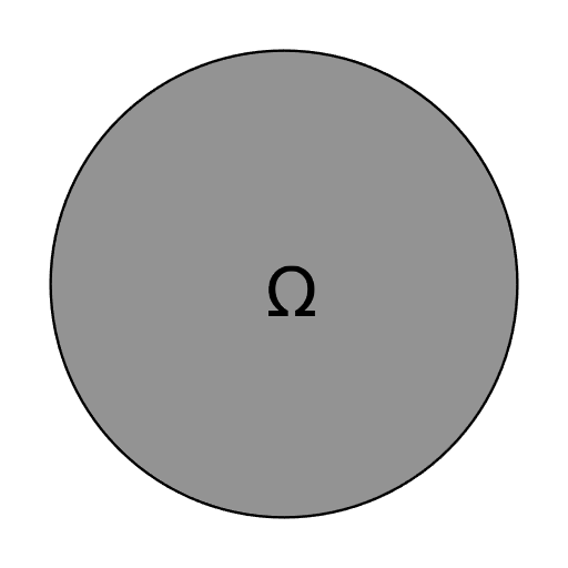
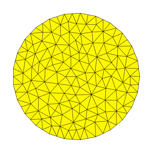
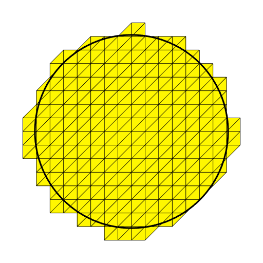
Figure 1: Left: considered domain for the first test case. Center: a conforming mesh for the standard FEM. Right: a uniform Cartesian mesh for $\phi$-FEM.

Moreover, we consider the manufactured solution given by $u_{\text{ref}}=\cos\left(\frac{1}{2}\pi(x^{2}+y^{2})\right)\exp(x)\sin(t)$ so that $u_{\text{ref}}$ satisfies $u_{\text{ref}}(t=0)=u_{\text{ref}}^{0}=0$ and $u_{\text{ref}}=0$ on $\Gamma\times(0,T)$. Here, $\Omega_{\text{ref}}=\Omega_{h}$. We represent the errors in $l^{2}(H^{1})$ norm on Fig. 2 and in $l^{\infty}(L^{2})$ norm on Fig. 3, both with $\mathbb{P}_{1}$ and $\mathbb{P}_{2}$ finite elements ($k=1$ and $k=2$). Here, the numerical results fit well the theoretical convergence order of Theorem 1 and behaves even better since we observe a convergence of orders two and three for the $l^{\infty}(L^{2})$ norm instead of $1.5$ and $2.5$ respectively. We remark that the theoretical constraint $\Delta t\geqslant ch^{2}$ is not satisfied for the $\mathbb{P}^{2}$ finite elements but it does not affect the practical convergence. We also represent the $l^{2}(H^{1})$ and $l^{\infty}(L^{2})$ errors with respect to the computation time (here, the computation time is the sum of time needed to assemble the finite element matrix and to solve the finite element systems at each time step, without the time used to construct the meshes) in Fig. 4. We observe that in this case, $\phi$-FEM is significantly faster than a standard FEM to obtain a solution with the same precision.

In Fig. 5 (left), we represent the $l^{2}(H^{1})$ error and in Fig. 5 (right) the $l^{\infty}(L^{2})$ error, both with respect to $\sigma$. This allows us to emphasize the influence of $\sigma$ on the stability of the errors and validates our choice of $\sigma=1$ in the other simulations.

Finally, in Fig. 6, we justify our choice for the degree of interpolation of $\phi$ since in our theoretical result, $\mathbb{P}_{k}$ is sufficient but we observe here that the error decreases for $l=2$. Furthermore, in our previous paper [7], our theoretical results in the Neumann case hold true only for $l\geq k+1$. Here, since the interpolation is exact from $l=2$ we do not need to compute highest degrees of interpolation for the level-set function to compare the results.

Figure 2: First test case. $l^{2}(0,T;H^{1}(\Omega))$ relative errors with respect to $h$ with ${P}_{1}$ elements and $\Delta t=h$ (left) and with ${P}_{2}$ elements and $\Delta t=h^{2}$ (right). Standard FEM (red squares) and $\phi$-FEM (blue dots), $\sigma=1$.

Figure 3: First test case. $l^{\infty}(0,T;L^{2}(\Omega))$ relative errors with respect to $h$ with ${P}_{1}$ elements and $\Delta t=h^{2}$ (left) and with ${P}_{2}$ elements and $\Delta t=h^{3}$ (right). Standard FEM (red squares) and $\phi$-FEM (blue dots), $\sigma=1$.

Figure 4: First test case. $l^{2}(0,T;H^{1}(\Omega))$ with $\Delta t=h$ (left) and $l^{\infty}(0,T;L^{2}(\Omega))$ with $\Delta t=h^{2}$ (right) relative errors with respect to the computation time. Standard FEM (red squares) and $\phi$-FEM (blue dots), ${P}_{1}$ elements, $\sigma=1$.

Figure 5: First test case. $l^{2}(0,T;H^{1}(\Omega))$ relative errors with respect to $\sigma$ for different mesh sizes, with $\Delta t=h$ (left) and $l^{\infty}(0,T;L^{2}(\Omega))$ relative errors with respect to $\sigma$, $\Delta t=h^{2}$ (right), both with ${P}_{1}$ elements.

Figure 6: First test case. $l^{2}(0,T;H^{1}(\Omega))$ relative errors with respect to $h$ for different values of $l$, $\Delta t=h$ (left) and $l^{\infty}(0,T;L^{2}(\Omega))$ relative errors with respect to $h$ for different values of $l$, $\Delta t=h^{2}$ (right), both with ${P}_{1}$ elements and $\sigma=1$.

Second test case : the source term is given and the FEM solution is compared to a standard FEM solution on a very fine mesh.

We now consider a more realistic test case since we will apply some forces and consider the resulting distribution of heat in the considered domain. More precisely, this time, we impose $u=0$ on $\Gamma\times(0,T)$, the initial condition is $u^{0}=0$ in $\Omega$ and we define a source term given by $f(x,y,z,t)=\exp\left(-\frac{(x-\mu_{1})^{2}+(y-\mu_{2})^{2}+(z-\mu_{3})^{2}}{2\sigma_{0}^{2}}\right)$ for each $(x,y,z,t)\in\Omega\times(0,T)$, with $(\mu_{1},\mu_{2},\mu_{3},\sigma_{0})=(0.2,0.3,-0.1,0.3)$. The final time is fixed to $T=1$. Moreover, for this test case, we will consider a more complex and 3D domain from [15], given by

$$\phi(x,y,z)=x^{2}+y^{2}+z^{2}-r_{0}^{2}-A\sum_{k=0}^{11}\exp\left(-\frac{(x-x_{k})^{2}+(y-y_{k})^{2}+(z-z_{k})^{2}}{\sigma^{2}_{0}}\right)\,,$$

with

$$(x_{k},y_{k},z_{k}) =\frac{r_{0}}{\sqrt{5}}\left(2\cos\left(\frac{2k\pi}{5}\right),2\sin\left(\frac{2k\pi}{5}\right),1\right)\,,\quad\hfill 0\leqslant k\leqslant 4\,,$$

$$(x_{k},y_{k},z_{k}) =\frac{r_{0}}{\sqrt{5}}\left(2\cos\left(\frac{(2(k-5)-1)\pi}{5}\right),2\sin\left(\frac{(2(k-5)-1)\pi}{5}\right),-1\right)\,,\quad\hfill 5\leqslant k\leqslant 9\,,$$

$$(x_{k},y_{k},z_{k}) =\left(0,0,r_{0}\right)\,,\quad\hfill k=10\,,$$

$$(x_{k},y_{k},z_{k}) =\left(0,0,-r_{0}\right)\,,\quad\hfill k=11\,,$$

with $r_{0}=0.6$, $\sigma=0.3$ and $A=1.5$. The resulting domain and meshes are given in Fig. 7.

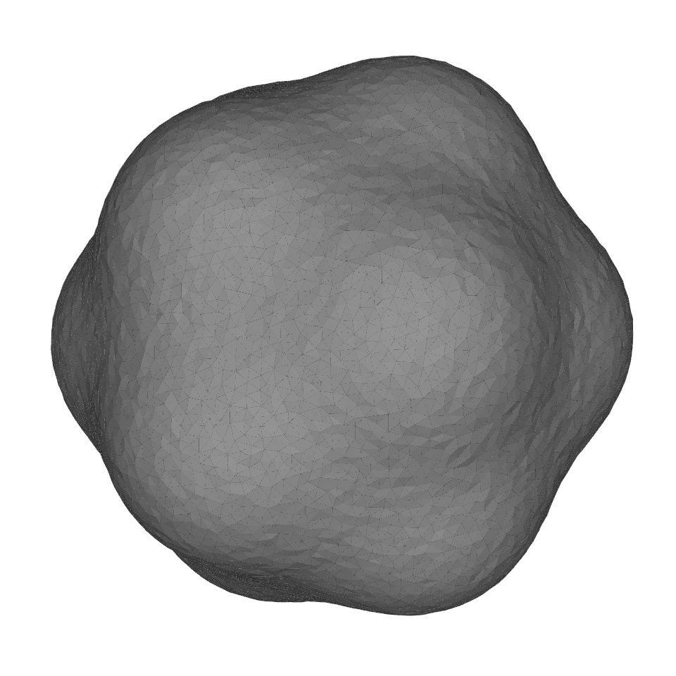
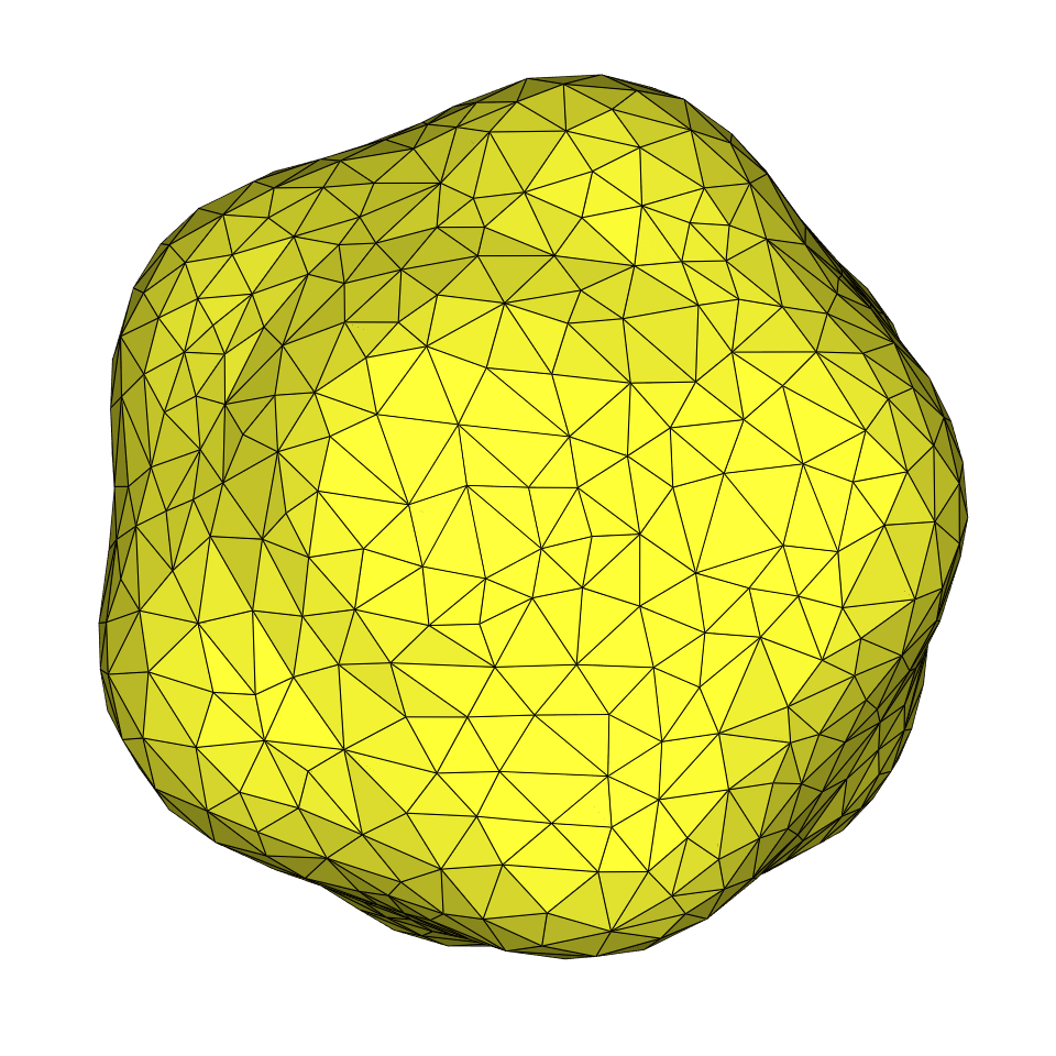
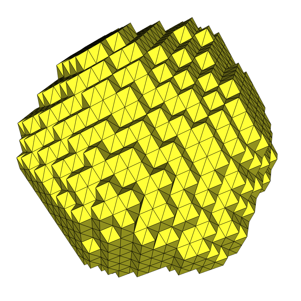
Figure 7: Left: considered domain for the second test case. Center: a conforming mesh for the standard FEM. Right: a uniform Cartesian mesh for $\phi$-FEM.

Here, $u_{\text{ref}}$ denotes the solution of a classical finite element method on $\Omega_{\text{ref}}$ that is a very fine conforming mesh. In this case, to be more precise, we introduce a partition of the interval $[0,T]$ into time steps $0=t^{\text{ref}}_{0}<t^{\text{ref}}_{1}<\dots<t^{\text{ref}}_{M}=T$ with $t^{\text{ref}}_{n}=n\Delta t^{\text{ref}}$ and $\Delta t^{\text{ref}}=h^{p/m}_{\text{ref}}$, where $h_{\text{ref}}$ denotes the size of cells of $\Omega_{\text{ref}}$. Then, in the numerical simulations each discretization is built so that $\left\{t_{n}\right\}_{n=0,\dots,N}$ is a subset of $\left\{t_{n}^{\text{ref}}\right\}_{n=0,\dots,M}$. In Fig. 8, we consider $\mathbb{P}_{1}$ finite elements ($k=1$), and ${P}_{2}$ finite elements for the interpolation $\phi_{h}$ of $\phi$ ($l=2$). We compare here the $l^{2}(H^{1})$, $l^{\infty}(L^{2})$ relative errors between the solution of the $\phi$-FEM scheme (4) and a standard FEM. The numerical results fit well the theoretical convergence order announced in Theorem 1, namely, order one for the $l^{2}(H^{1})$ norm and order two for the $l^{\infty}(L^{2})$ error.

Figure 8: Second test case. $l^{2}(0,T;H^{1}(\Omega))$ relative errors with respect to $h$ with $\Delta t=h$ (left) and $l^{\infty}(0,T;L^{2}(\Omega))$ relative errors with respect to $h$ with $\Delta t=h^{2}$ (right), both with ${P}_{1}$ elements. Standard FEM (red squares) and $\phi$-FEM (blue dots), $\sigma=1$.

4 Conclusion

In the present work, we proposed a FEM scheme following the $\phi$-FEM paradigm to approximate the solution of the heat equation and proved its convergence, which is optimal in the $l^{2}(0,T;H^{1}(\Omega))$ norm and quasi-optimal in the $l^{\infty}(0,T;L^{2}(\Omega))$ norm. We remark that, in comparison with [6], we need less regularity on the exact solution in the a priori error estimates.

A first advantage of the $\phi$-FEM paradigm is its ease of implementation. Indeed, it uses standard shape functions contrary to the XFEM approach. Moreover, it uses standard integration tools contrary to cutFEM needing an integration on the real boundary and some integrations on cut cells.

A second interesting aspect of our approach is the computational time of the simulation. The low cost (computational time) of $\phi$-FEM can be explained by the fact that the boundary of the geometry in the classical finite element method is approximated by some linear functions while, in the $\phi$-FEM paradigm, the boundary is taken into account thanks to the level set function $\phi$, which can be of high degree without increasing the size of the finite element matrix.

In the mathematical analysis, we supposed that the boundary of the considered domain is regular enough. The case of less regular domains will be the aim of future work.

Funding

This work was supported by the Agence Nationale de la Recherche, Project PhiFEM, under grant ANR-22- CE46-0003-01.

References

- [1] Vidar Thomée. Galerkin finite element methods for parabolic problems, volume 25 of Springer Series in Computational Mathematics. Springer-Verlag, Berlin, 1997.
- [2] R. Glowinski, T. Pan, and J. Periaux. A fictitious domain method for Dirichlet problem and applications. Computer Methods in Applied Mechanics and Engineering, 111(3-4):283–303, 1994.
- [3] R. Mittal and G. Iaccarino. Immersed boundary methods. Annu. Rev. Fluid Mech., 37:239–261, 2005.
- [4] C. Annavarapu, M. Hautefeuille, and J. Dolbow. A robust Nitsche’s formulation for interface problems. Computer Methods in Applied Mechanics and Engineering, 225-228:44–54, 2012.
- [5] A. Main and G. Scovazzi. The shifted boundary method for embedded domain computations. Part I: Poisson and Stokes problems. J. Comput. Phys., 372:972–995, 2018.
- [6] M. Duprez and A. Lozinski. -FEM: a finite element method on domains defined by level-sets. SIAM J. Numer. Anal., 58(2):1008–1028, 2020.
- [7] Michel Duprez, Vanessa Lleras, and Alexei Lozinski. A new -FEM approach for problems with natural boundary conditions. Numerical Methods for Partial Differential Equations, 39(1):281–303, 2023.
- [8] Stéphane Cotin, Michel Duprez, Vanessa Lleras, Alexei Lozinski, and Killian Vuillemot. -FEM: an efficient simulation tool using simple meshes for problems in structure mechanics and heat transfer. In Partition of Unity Methods (Wiley Series in Computational Mechanics) 1st Edition. Wiley, Nov 2022.
- [9] Peter Schwartz, Michael Barad, Phillip Colella, and Terry Ligocki. A Cartesian grid embedded boundary method for the heat equation and Poisson’s equation in three dimensions. J. Comput. Phys., 211(2):531–550, 2006.
- [10] Peter McCorquodale, Phillip Colella, and Hans Johansen. A Cartesian grid embedded boundary method for the heat equation on irregular domains. J. Comput. Phys., 173(2):620–635, 2001.
- [11] E. Burman. Ghost penalty. C. R. Math. Acad. Sci. Paris, 348(21-22):1217–1220, 2010.
- [12] Lawrence C Evans. Partial differential equations, volume 19. American Mathematical Soc., 2010.
- [13] Michel Duprez, Vanessa Lleras, and Alexei Lozinski. -FEM: an optimally convergent and easily implementable immersed boundary method for particulate flows and Stokes equations. accepted paper, M2AN, 2022.
- [14] M Alnæs, J Blechta, J Hake, A Johansson, B Kehlet, A Logg, C Richardson, J Ring, ME Rognes, and GN Wells. Archive of numerical software: The fenics project version 1.5. University Library Heidelberg, 2015.
- [15] E. Burman, S. Claus, P. Hansbo, M. Larson, and A. Massing. Cutfem: discretizing geometry and partial differential equations. International Journal for Numerical Methods in Engineering, 104(7):472–501, 2015.